Topological insulators on a Mobius Strip

Abstract

We study the two dimensional Chern insulator and spin Hall insulator on a non-orientable Riemann surface, the Mobius strip, where the usual bandstructure topological invariant is not defined. We show that while the flow pattern of edge currents can detect the twist of the Mobius strip in the case of Chern insulator, it can not do so in spin Hall insulator.

Band insulator with interesting bandstructure topology, the so called “topological insulator”, has attracted considerable attention latelytopo . Mathematically these free-electron insulators are characterized by topological invariants in their bandstructure. Examples include the Chern numberTKNN ; qi and $Z_{2}$ indexkm ; moore ; roy ; kane for the Chern and $Z_{2}$ insulator, respectively. Physically a hallmark of these insulators is their protected boundary states. In two dimensions these are the chiral edge states of the integer quantum Hall effecthalperin ; hatsugai , and the helical edge states of the spin Hall insulatorzb ; konig . In three dimensions the boundary states have a massless Dirac fermion dispersion relationfkm ; arpes .

In this paper we ask a simple question: in two dimensions can we put topological insulators on a non-orientable Riemann surface? and if so, what are their signatures? The first question was posed to us by Prof. X. Sun of the Fudan University. Clearly the usual bandstructure topological invariants can not be defined in this situation; therefore naturally one would examine the edge state structure. In the following we study two dimensional Chern and $Z_{2}$ insulator on the Mobius strip. Since the Mobius strip has only one edge, it is far from clear how does the flow pattern of the current look like.

First we start with the Chern insulator. As pointed out by HaldaneHaldane_prl1988 , the necessary ingredient of Chern insulator is time-reversal symmetry breaking rather than net magnetic flux. Specifically we consider the following two-band model on square lattice

$$\mathcal{H}\left({\bf k}\right)={\bf d}({\bf k})\cdot\vec{\tau}.$$ (1)

Here $\vec{\tau}$ are Pauli matrices which acts on the (two) orbital degrees of freedom, and

$${\bf d}({\bf k})=(\sin k_{x},\sin k_{y},1-\cos k_{x}-\cos k_{y}).$$ (2)

It is straightforward to check that the Chern number (or the TKKN index) associated with the valence band of this model is $1$. In order to implement this model on the Mobius strip we first need to Fourier transform the above model to real space:

$$H=-\frac{1}{2}\sum_{i,j}\left[i(\psi_{i+1,j}^{\dagger}\tau_{x}\psi_{i,j}+\psi_{i,j+1}^{\dagger}\tau_{y}\psi_{i,j})+\psi_{i+1,j}^{\dagger}\tau_{z}\psi_{i,j}+\psi_{i,j+1}^{\dagger}\tau_{z}\psi_{i,j}+h.c.\right]+\sum_{i,j}\psi_{i,j}^{\dagger}\tau_{z}\psi_{i,j}.$$ (3)

In the above $(i,j)$ are the integer coordinates of the sites of a square lattice, and $\psi$ is a two-component fermion field associated with the two orbitals in question. Because we shall study Eq. (3) on the Mobius strip it is essential to define how do the orbitals couple to the local orientation. A convenient definition is to let the pseudospin corresponding to the orbital degrees of freedom couple to curvature in the same way the real spin in Dirac theory doeslee . This amounts to replacing the $\tau$ matrices in Eq. (3) by the following position-dependent Pauli matrices, i.e.,

$$\tau_{\mu}\Rightarrow\vec{\tau}_{i,j;\mu}=\hat{n}_{i,j;\mu}\cdot\vec{\tau}.$$ (4)

Here $\mu=1,2,3$ and $\hat{n}_{ij,\mu}$ are unit vectors defining a local frame when the relevant surface is embedded in the three dimensional Euclidean space ($\hat{n}_{3}$ is the local surface normal).

Let us warm up by studying the surface of a cylinder. We build a coordinate system as follows:

$$x(u,v)=\cos u,~{}y(u,v)=\sin u,~{}z(u,v)=v.$$ (5)

where $0\leq u<2\pi$ and $-1\leq v\leq 1$. Thus we have a cylinder of height 2 and radius 1. The local frame is defined by

$$\hat{n}_{1}(u,v)=\partial_{v}\vec{r}(u,v)$$

$$\hat{n}_{2}(u,v)=\partial_{u}\vec{r}(u,v)$$

$$\hat{n}_{3}(u,v)=\hat{n}_{1}(u,v)\times\hat{n}_{2}(u,v),$$ (6)

where $\vec{r}(u,v)=(\cos u,\sin u,v)$. Set $u,v$ to a set of discrete values corresponding to the square lattice we substitute Eq. (6) into Eq. (4) then Eq. (3). We diagonalize the resulting Hamiltonian numerically and compute the expectation value of the current operator.

$$j_{1,2}=\psi_{i,j}^{\dagger}\tau_{i,j;1,2}\psi_{i,j}.$$ (7)

In Fig. (1) we plot the result. As expected counter-propagating chiral edge currents are found on the two opposite edges.

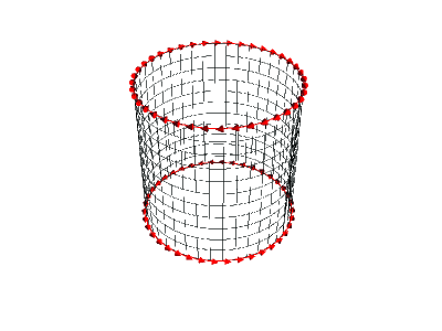
Figure 1: (color on-line) The edge current associated with the Chern insulator described in the text. There are 40/12 sites in the circumferential and height directions respectively. The direction of the current is illustrated by the red arrows. The length of arrows is proportional to the magnitude of the current. To make the plot easier to understand we have omitted the weak current away from the edge.

Now we are ready for the Mobius strip. The coordinate system we use is

$$x(u,v)=\left(1+\frac{v}{2}\cos\frac{u}{2}\right)\cos u$$

$$y(u,v)=\left(1+\frac{v}{2}\cos\frac{u}{2}\right)\sin u$$

$$z(u,v)=\frac{v}{2}\sin\frac{u}{2}.$$ (8)

In Fig. (2) we first present the result when all bonds across a line segment are removed.

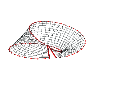
Figure 2: (color on-line) The edge current associated with the Chern insulator on a Mobius strip. There are $40\times 12$ sites, and all bonds across a line segment are removed. Again, to make the plot easier to understand we have omitted the weak current away from the edge.

We note that a pair of co-propagating edge currents are localized on the cut. Their presence is due to the orientation flip across the cut. As a result the chirality of the Chern insulator reverses across the cut. This is similar to the edge current produced at the location of magnetic field reversal in the quantum Hall effect. Because the edge currents at the cut are co-propagating, seal the cut has no effect on them. The current pattern after the cut is sealed is shown in Fig. (3).

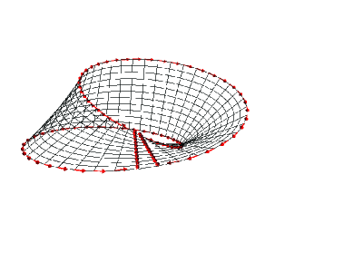
Figure 3: (color on-line) The edge current associated with the Chern insulator on a Mobius strip. There are $40\times 12$ sites. To make the plot easier to understand we have omitted the weak current away from the edge.

It is worthy to note that while geometrically there is no singularity on a Mobius strip, in defining the chirality of the Chern insulator it is necessary to choose a cut across which the direction reverses. Thus the current pattern of the Chern insulator does detect the twist of the Mobius strip.

Next we study the $Z_{2}$ insulator on the Mobius strip. The momentum space Hamiltonian in $\mathbb{R}^{2}$ is given by

$$\mathcal{H}\left({\bf k}\right)=d_{1}({\bf k})\tau_{1}\otimes I_{2}+d_{2}({\bf k})\tau_{2}\otimes I_{2}+d_{3}({\bf k})\tau_{3}\otimes{\sigma}_{3},$$ (9)

where $I_{2}$ is the $2\times 2$ identity matrix. The corresponding real space version is

$$H = -\frac{1}{2}\sum_{i,j}\left[i(\psi_{i+1,j}^{\dagger}\tau_{x}\otimes I_{2}\psi_{i,j}+\psi_{i,j+1}^{\dagger}\tau_{y}\otimes I_{2}\psi_{i,j})+\psi_{i+1,j}^{\dagger}\tau_{z}\otimes{\sigma}_{z}\psi_{i,j}+\psi_{i,j+1}^{\dagger}\tau_{z}\otimes{\sigma}_{z}\psi_{i,j}+h.c.\right]$$ (10)

$$+ \sum_{i,j}\psi_{i,j}^{\dagger}\tau_{z}\otimes{\sigma}_{z}\psi_{i,j}.$$

In defining Eq. (10) on the Mobius strip we define the local spin Pauli matrices, $\sigma_{i,j;\mu}$, in the same way in Eq. (4). We also start by studying the edge current pattern on the cylinder. As shown in Fig. (4) there are a pair of time-reversal conjugate, counter-propagating edge currents at each edge. Here blue arrows indicate the direction of local $S_{z}$ axis. The red arrows at the top/bottom of the blue ones illustrate the current associated with $S_{z}=\pm 1$, respectively.

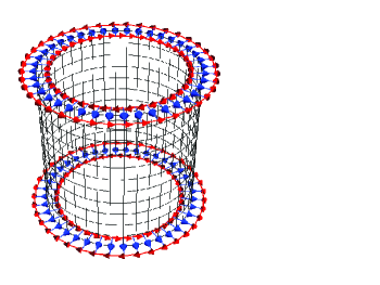
Figure 4: (color on-line) The edge current associated with the $Z_{2}$ insulator on a Mobius strip. The blue arrows indicate the direction of local $S_{z}$ axis.The red arrows at the top/bottom of the blue ones illustrate the current associated with $S_{z}=\pm 1$, respectively. There are $40\times 12$ sites, and to make the plot easier to understand we have omitted the weak current away from the edge.

At last we study the $Z_{2}$ insulator on the Mobius strip. Again, we begin by removing the bonds across a line segment. The associated current pattern is shown in Fig. (5). The meaning of blue and red arrows are the same as in Fig. (4). The inset zooms in at the currents near the cut.

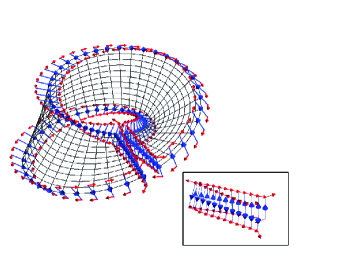
Figure 5: (color on-line) The edge current associated with the $Z_{2}$ insulator on a Mobius strip. Bonds across a line segment are removed. The meaning of blue and red arrows are the same as in Fig. (4). There are $40\times 12$ sites, and to make the plot easier to understand we have omitted the weak current away from the edge. The inset zooms in at the currents near the cut. Note for each spin component there is a pair of counter-propagating current.

It is important to note that for each spin component there is a pair of counter-propagating current. As the result, when the cut is sealed they are allowed to back scatter against each other and hence gaps out the associated edge modes. The result with the cut sealed is shown in Fig. (6). As expected the edge currents associated with the cut are completely removed.

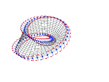
Figure 6: (color on-line) The edge current associated with the $Z_{2}$ insulator on a Mobius strip. The meaning of blue and red arrows are the same as in Fig. (4). There are $40\times 12$ sites, and too make the plot easier to understand we have omitted the weak current away from the edge.

In summary we have studied the edge current distribution of the Chern and $Z_{2}$ insulators on the Mobius strip. The current pattern of the Chern insulator clearly detects the twist, while that of the $Z_{2}$ insulator does not. This reveals an interesting interaction between the topology of the electronic structure and that of the substrate. The fact that the $Z_{2}$ topological insulator can be seamlessly put on a $Z_{2}$ fiber bundle (the Mobius strip is a $Z_{2}$ fiber bundle over a circle) is particularly interesting. The mathematical meting of this needs to be clarified in the future.

Acknowledgment: We thank Hong Yao for helpful discussions. LTH is supported by the NSFC Grant No. 11074143, and the Program of Basic Research Development of China Grant No. 2011CB921901. LTH also acknowledges the support of China Scholarship Council and the Doctoral Short-Term Visiting-Abroad Foundation of Tsinghua University, Beijing. DHL is supported by DOE grant number DE-AC02-05CH11231.

References

- (1) J. Moore, Nature Physcs, 5 378 (2009); M.Z. Hasan, MZ and C.L. Kane, Rev. Mod. Phys. 82, 3045 (2010); X.-L. Qi and S.-C.Zhang, Physics Today, 63, 33 (2010).
- (2) D. J. Thouless, M. Kohmoto, M. P. Nightingale, and M. den Nijs 49, 405 (1982).
- (3) X.-L. Qi, T. L. Hughes, and S.-C. Zhang, Phys. Rev. B 78, 195424 (2008).
- (4) C. L. Kane and E. J. Mele, Phys. Rev. Lett. 95, 226801 (2005); C. L. Kane and E. J. Mele, Phys. Rev. Lett. 95, 146802 (2005).
- (5) J.E. Moore, L. Balents, Phys. Rev. B 75, 121306(R) (2007).
- (6) R. Roy, Phys. Rev. B 79, 195322 (2009).
- (7) L.Fu, C. L. Kane, and E. J. Mele, Phys. Rev. Lett. 98, 106803 (2007); L. Fu and C. L. Kane, Phys. Rev. B 76, 045302 (2007).
- (8) B. I. Halperin Phys. Rev. B 25, 2185 (1982)
- (9) Yasuhiro Hatsugai Phys. Rev. Lett. 71, 3697 (1993).
- (10) B. A. Bernevig, T. L. Hughes, and S.-C. Zhang, Science 314, 1757 (2006).
- (11) M. Konig, S. Wiedmann, C. Brune, A. Roth, H. Buhmann, L.W. Molenkamp, X.-L. Qi, S.-C. Zhang, Science, 318, 766, (2007).
- (12) L. Fu, C.L. Kane, and E.J. Mele, Phys. Rev. Lett. 98, 106803 (2007).
- (13) D. Hsieh et al., Nature 452, 970 (2008); D. Hsieh et al., Science 323, 919 (2009); Y. Xia et al., Nature Physics 5, 398 (2009); Y. L. Chen et al., Science, 1173034 (June 11, 2009).
- (14) F. D. M. Haldane Phys. Rev. Lett. 61, 2015 (1988).
- (15) D.-H. Lee, Phys. Rev. Lett. 103,196804, (2009).