Neutral stability height correction for ocean winds

Abstract

Adjusting ocean wind observations to a standard height, usually $\mathrm{{10}\mbox{{~{}}}{m}}$, requires the use of a boundary layer model, and knowledge of the thermodynamical variables. Height adjustment is complicated by the fact that a necessary parameter, the roughness height, cannot be given in a closed form solution. If only the wind and reporting height are known, the best that can be done is to assume neutral stability. The determination of roughness height is analyzed and a simple approximation (used by Atlas et al. 2011) is derived in detail. This approximation is accurate for winds in the range of $\mathrm{{{1-30}}\mbox{{~{}}}{m\;s^{-1}}}$ for neutral stratification and would be an excellent initial estimate for a Newton iteration to determine the roughness height precisely, whether or not neutral stability is assumed.

1 Introduction

Adjusting ocean wind observations to a standard height, usually $\mathrm{{10}\mbox{{~{}}}{m}}$, requires the use of a boundary layer model, and knowledge of the thermodynamical variables. Whichever PBL model is used, an exact solution requires iterating the constant flux layer equations. This is due to the fact that $z_{0}$, the roughness length, is an implicit function of the model variables over the oceans. The Charnock formula states that over the ocean $z_{0}$ and the surface stress magnitude $|\tau|$ are linearly related by

$$\mbox{$z_{0}$}=\frac{a}{\rho g}|\tau|.$$ (1)

Here $a=0.0185$ is the Charnock constant, $\mathrm{{g=9.81}\mbox{{~{}}}{m\;s^{-2}}}$, and $\rho$, the density of air, is assumed to be constant for the range of heights considered and equal to its surface value. Previously $a=0.032$ was the accepted value for the Charnock constant, but now it is known the Charnock constant is not actually a constant, but depends on the sea state, through the wave age (Wu 1985). Accordingly, the Charnock constant is determined by the wave model in the ECMWF system, and normally is in the range $0.01\leq a\leq 0.04$, corresponding to sea states from swell to steep young ocean waves (Hersbach 2011). While values of $a$ as large as 0.1 sometimes occur in the ECMWF system, a typical value is $a=0.018$, which agrees with the value of 0.0185 used here and by Wu (1985). Note that Eq. (1) neglects the contribution of molecular viscosity which is important at low wind speeds (e.g., Hersbach 2011). However, at low wind speeds the height correction and consequently errors made in the height correction should be small.

Surface stress determined from

$$\tau=-\rho C_{d}|V|V$$ (2)

also depends on $z_{0}$ through the neutral drag coefficient, and in the unstable case through the similarity function, usually denoted $f(Ri)$ where $Ri$ is the Richardson number. In Eq. (2) $V$ is the vector wind at some height $z$, $|V|$ is the magnitude of the vector wind, the wind and stress vectors are assumed to be parallel for the range of heights considered, and the drag coefficient $C_{d}$ is given by the product of the similarity function $f(Ri)$ and the neutral drag coefficient

$$C_{dn}=\left[\frac{k}{\log\left(\frac{\displaystyle z}{\mbox{$z_{0}$}}\right)}\right]^{2}.$$ (3)

Here the von Kármán constant $k=0.4$. See Hoffman and Louis (1990) for details.

NWP models usually “cheat” and use the value of $\tau$ of the previous time step to find $z_{0}$ through the Charnock formula. Actually using old values to evaluate the dissipative terms can be a good policy as this can reduce computational instability. But outside of a model we must calculate $z_{0}$ implicitly. For this purpose we substitute the absolute value of Eq. (2) into Eq. (1) and then use the expresseion for $C_{d}$ to obtain

$$\mbox{$z_{0}$}=\frac{a}{g}C_{d}|V|^{2}=\frac{a}{g}f(Ri)\left[\frac{k|V|}{\log\left(\frac{\displaystyle z}{\mbox{$z_{0}$}}\right)}\right]^{2}\equiv h(\mbox{$z_{0}$};|V|,z,Ri).$$ (4)

For neutral stratification, $Ri=0$, and $f(Ri)=1$. To solve Eq. (4) we must iterate. To begin the process, Hoffman and Louis (1990) estimated $C_{d}$ as a linear function of $|V|$ and then obtained the initial estimate of $z_{0}$ from the Charnock relationship. Then Eq. (4), $\mbox{$z_{0}$}=h$, is iterated. This converges to a good approximation within a few iterations. It is then possible to switch to a Newton iteration to solve $\mbox{$z_{0}$}-h\equiv f(\mbox{$z_{0}$})=0$. The Newton method requires the partial derivative of $h$ with respect to $z_{0}$. This can be evaluated using the tangent linear code corresponding to the calculation of $h$ by setting all inputs to zero except for that corresponding to $z_{0}$, which is set to unity. The advantage of the Newton method is that it iterates to machine precision in 2-4 steps from a reasonable start. (With an unreasonable start it can diverge.) With a solution exact to machine precision one can then skip the iteration in the adjoint and/or tangent models. As an alternative within the context of the ECMWF system, Hersbach (2011) describes an accurate fit for $C_{dn}$ and $z_{0}$ as functions of neutral wind speed and the Charnock value, two parameters available in the interface between the ECMWF atmospheric and wave models.

2 Height correction for ocean winds

Knowing $z_{0}$ is equivalent to knowing the stress, and we can then solve Eq. (4) for $|V|$ at any height, $z$, if only we know the Richardson number. In particular, Eq. (4) states that $C_{d}^{\frac{1}{2}}|V|$ is conserved as we vary the height $z$. However $Ri$ depends on knowing the stratification of the boundary layer. In what follows we assume that only the wind and reporting height are known. Then the best that can be done is to assume neutral stability, and in the rest of this treatment $V$ will denote the neutral stability wind. Now, $C_{dn}^{\frac{1}{2}}|V|$ is conserved, allowing us to determine the $\mathrm{{10}\mbox{{~{}}}{m}}$ neutral wind speed $|V_{10}|$ from an observation at some other height according to:

$$|V_{10}|=\left[\frac{\log(10/\mbox{$z_{0}$})}{\log(z/\mbox{$z_{0}$})}\right]|V|.$$ (5)

Note that according to Eq. (5), the ratio between neutral stability winds at two levels is entirely determined by $z_{0}$ and the two heights.

Once $z_{0}$ is determined, the neutral wind, defined by

$$\tau=-\rho C_{dn}|V|V,$$ (6)

is easily determined from knowledge of $z_{0}$ alone according to

$$V=\left(\frac{g}{ak^{2}}\right)^{\frac{1}{2}}\mbox{$z_{0}$}^{\frac{1}{2}}\log\left(\frac{z}{\mbox{$z_{0}$}}\right),$$ (7)

which is obtained by combining Eq. (6) with Eq. (1) and making use of Eq. (3). A few sample calculations using Eq. (7) are presented in Table 1 for heights of 4, 10, and $\mathrm{{19.5}\mbox{{~{}}}{m}}$. In Table 1 we see that the variation in $z_{0}$ is two orders of magnitude greater than the variation in wind speed. Over this range of wind speed, the correction factors for determining $|V_{10}|$ vary by as much as 5%. This variation is the same order of magnitude as the corrections, and is therefore worth accounting for.

Table 1: Sample calculations based on Eq. (7). The $z_{0}$ values are equal to $2^{-j}$ but have been multiplied by 10⁶ for presentation in this table. The $|V_{10}|$ values are in $\mathrm{{{}}\mbox{{~{}}}{m\;s^{-1}}}$ and are calculated using Eq. (7). The ratios in columns 4 and 5 are equal to the term in square brackets in Eq. (5). The last column contains the estimated value of $z_{0}$ from Eq. (12).

$j$ $\mbox{$z_{0}$}\times 10^{6}$ $|V_{10}|$ $|V_{10}/V_{4}|$ $|V_{10}/V_{19.5}|$ $\hat{z}_{0}\times 10^{6}$ 14 61 5.4 1.08 0.947 68 11 488 12.6 1.10 0.937 493 8 3906 28.2 1.13 0.922 3216

3 Calculation of $z_{0}$ under neutral conditions

To apply Eq. (5) we still need to determine $z_{0}$. Here we demonstrate a simple approximation. The motivation is that under neutral conditions, for some fixed height, we expect wind speed, surface stress, and roughness height to all increase together. Differentiating Eq. (7), we obtain

$$\frac{d|V|}{d\mbox{$z_{0}$}}=\left(\frac{g}{ak^{2}}\right)^{\frac{1}{2}}\mbox{$z_{0}$}^{-\frac{1}{2}}\left[\frac{1}{2}\log\left(\frac{z}{\mbox{$z_{0}$}}\right)-1\right].$$ (8)

Thus $d|V|/d\mbox{$z_{0}$}/>0$ provided $z>e^{2}\mbox{$z_{0}$}$. This holds for wind speeds less than hurricane strength and heights of several meters or more. The suggestion then is that $z_{0}$ should be a monotonically increasing function of $|V|$, and interpolation into a look-up table, or a simple fit to a set of exact values should work.

For this investigation it is convenient to define

$$y=\log(z/\mbox{$z_{0}$})\quad\mbox{so that}\quad\mbox{$z_{0}$}=ze^{-y}.$$ (9)

Then the square of Eq. (7) may be written as

$$y^{2}e^{-y}\equiv\gamma=\frac{ak^{2}}{gz}V^{2}.$$ (10)

Usually we will know $V$ and $z$ and hence $\gamma$ from Eq. (10). From $\gamma$ we then determine $y$ and finally $z_{0}$ from Eq. (9). To determine $y$ from $\gamma$ we tabulate or model $y$ as a function of $\gamma$, based on data obtained by calculating $\gamma$ from Eq. (10) for different values of $y$. Note that the values of the regression coefficients determined below are independent of the value of $z$ or any of the other parameters, including the Charnock constant $a$. However, to create a relevant sample of $y$-values for fitting, we take $\mathrm{{z=10}\mbox{{~{}}}{m}}$, and vary $z_{0}$. Below, as in Table 1, we take values of $z_{0}$ evenly distributed in log space given by $2^{-j}$ for integer values of $j$.

Figure 1a plots $y$ as a function of $\log(\gamma)$ for $j=0,\ldots,30$. Clearly a linear fit will work well over most the range of $\gamma$. This is not unexpected since according to Eq. (10) $\log\gamma=-y+2\log y$. As $j$ increases, $z_{0}$, $|V_{10}|$, and $\gamma$ decrease, while $y$ increases. For example, for $j=0$, $\mathrm{{\mbox{$z_{0}$}=1}\mbox{{~{}}}{m}}$ and $\mathrm{{{|V_{10}|=134}}\mbox{{~{}}}{m\;s^{-1}}}$, while for $j=30$, $\mathrm{{\mbox{$z_{0}$}\approx 10^{-9}}\mbox{{~{}}}{m}}$ and $\mathrm{{{|V_{10}|=0.04}}\mbox{{~{}}}{m\;s^{-1}}}$. Fitting points for $j\geq 6$, corresponding to $\mathrm{{{|V_{10}|\leq 40}}\mbox{{~{}}}{m\;s^{-1}}}$ (where the extreme point included is marked by the vertical line in the plots) we find that

$$y=c_{0}+c_{1}\log(\gamma)$$ (11)

with $c_{0}=3.7$ and $c_{1}=-1.165$.

Combining Eq. (9), Eq. (10), and Eq. (11), we obtain our estimate of $z_{0}$

$$\hat{z}_{0}=z\exp[-(c_{0}+c_{1}\log[\gamma])]=z\exp[-(c_{0}+c_{1}\log[(ak^{2}V^{2})/(gz)])].$$ (12)

Figure 1b shows the error of the fit in log space. Values calculated using Eq. (12) are shown in the last column of Table 1 for the cases listed. The differences are not tiny, but when we recalculate the ratios of the wind speeds in columns 4 and 5 of the table, the results are nearly the same. Using the same precision as in the table, the values are the same except that the value for $|V_{10}/V_{19.5}|$ is 0.923.

Figure 1: Fitting $y=\log(z/\mbox{$z_{0}$})$ as a function of $\gamma=(ak^{2}/gz)V^{2}$. (a) The linear fit to values of $y$ and $\log\gamma$ for $j=6,\ldots,30$ is plotted as a dotted line. The data values are plotted as dots. (b) Log residuals for Eq. (12) fit of $z_{0}$. For this calculation we define the true values of $z_{0}$ and then $y$, $\gamma$ and $\hat{z}_{0}$ for the chosen value of $z$ ($\mathrm{{10}\mbox{{~{}}}{m}}$), using Eq. (9) and Eq. (12). The vertical lines identify $j=6$.

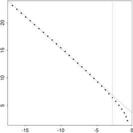
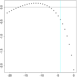
$y$ $\log\hat{z}_{0}-\log\mbox{$z_{0}$}$ a $\log\gamma$ b $\log\mbox{$z_{0}$}$

4 Concluding remarks

An approximation for roughness height (Eq. (12)) is given that is accurate for winds in the range of $\mathrm{{{1-30}}\mbox{{~{}}}{m\;s^{-1}}}$, assuming neutral stability and neglecting effects of molecular viscosity. (Also, note that coherent structures in the atmospheric boundary layer are not explicitly included in the similarity theory employed here.) Values of $z_{0}$ that vary with wind speed should be used in correcting ocean winds to a standard height. Typical corrections are in the range of 5-15%, so assuming a single value for $z_{0}$ will incur errors of a few per cent. Our approximation is also an excellent initial estimate to begin a Newton iteration to determine the roughness height precisely, whether or not neutral stability is assumed.

In practice, the approximation derived here is adequate because errors due to other approximations and assumptions are graver. For example, observations and meta-data associated with ship reports are often limited: information required to estimate atmospheric boundary layer stability may be lacking, anemometer heights may be unknown or incorrect, and effects due to ship motion and flow anomalies due to superstructure may not be accounted for.

Acknowledgement

The NASA Ocean Surface Wind Projects and the NASA Earth System Data Records Programs supported this work. Juan Carlos Jusem (Goddard Space Flight Center) and Zongpei Jiang (National Oceanography Centre, Southampton) provided helpful comments on the manuscript. A preliminary version of this study was posted to:
http://map.nasa.gov/data/ssw.old/reason_sample/doc/src/height-correct.pdf

References

- Atlas et al. (2011) Atlas, R., R. N. Hoffman, J. Ardizzone, S. M. Leidner, J. C. Jusem, D. K. Smith, and D. Gombos, 2011: A cross-calibrated, multi-platform ocean surface wind velocity product for meteorological and oceanographic applications. Bull. Amer. Meteor. Soc., 92 (2), 157–174, DOI:10.1175/2010BAMS2946.1.
- Hersbach (2011) Hersbach, H., 2011: Sea surface roughness and drag coefficient as functions of neutral wind speed. J. Phys. Oceanogr., 41 (1), 247–251, DOI:10.1175/2010JPO4567.1.
- Hoffman and Louis (1990) Hoffman, R. N. and J.-F. Louis, 1990: The influence of atmospheric stratification on scatterometer winds. J. Geophys. Res., 95 (C6), 9723–9730.
- Wu (1985) Wu, J., 1985: Parameterization of wind-stress coefficients over water surfaces. J. Geophys. Res., 90 (C5), 9069–9072.