Thermopower with broken time-reversal symmetry

Abstract

We show that when non-unitary noise effects are taken into account the thermopower is in general asymmetric under magnetic field reversal, even for non-interacting systems. Our findings are illustrated in the example of a three-dot ring structure pierced by an Aharonov-Bohm flux.

In power generation and refrigeration by means of thermal engines, efficiency plays a basic theoretical and practical role. The Carnot bound on efficiency lies at the foundations of thermodynamics: for a heat engine functioning between hot and cold reservoirs at temperatures $T_{h}$ and $T_{c}$, the efficiency $\eta$, defined as the ratio of the output power over the heat extracted per unit time from the high temperature reservoir, is upper bounded by the Carnot efficiency $\eta_{C}$: $\eta\leq\eta_{C}=1-T_{c}/T_{h}$.

For systems with time-reversal symmetry, thermoelectric power generation and refrigeration is governed, within linear response, by a single parameter, the dimensionless figure of merit $ZT=(\sigma S^{2}/\kappa)T$, where $\sigma$ is the electric conductivity, $S$ is the thermopower (Seebeck coefficient), $\kappa$ is the thermal conductivity, and $T\approx T_{h}\approx T_{c}$ is the temperature. The maximum efficiency is given by

$$\eta_{\rm max}=\eta_{C}\,\frac{\sqrt{ZT+1}-1}{\sqrt{ZT+1}+1}.$$ (1)

Thermodynamics only imposes $ZT\geq 0$ and the Carnot limit is reached when $ZT\to\infty$.

On the other hand, we have recently shown ZTmag that for systems with broken time-reversal symmetry the efficiency depends on two parameters: a “figure of merit” and an asymmetry parameter. In contrast to the time-symmetric case, the figure of merit is bounded from above; yet the Carnot efficiency can be reached at lower and lower values of the figure of merit as the asymmetry parameter increases. According to the expression for the efficiency, large asymmetry of the thermopower can be responsible for highly non-trivial effects ZTmag , and potentially can be a useful tuning parameter to control thermoelectric efficiency of the material. Hence, finding general conditions for asymmetry of the thermopower is of general interest both from practical and purely fundamental point of view.

If time-reversal symmetry is broken, e.g. by means of a magnetic field ${\bm{B}}$, then one does not expect the Seebeck coefficient to be in general symmetric with respect to the magnetic field. Yet for the particular case of non-interacting systems one has $S({\bm{B}})=S(-{\bm{B}})$ as a consequence of the symmetry properties of the scattering matrix datta . Even though this constraint does not apply when interactions or inelastic scattering are taken into account, and even though there are no general results imposing the symmetry of the Seebeck coefficient, the latter has always been found to be an even function of the magnetic field in purely metallic two-terminal mesoscopic systems vanlangen . On the other hand, Andreev interferometer experiments chandrasekhar and recent theoretical studies indicate that systems in contact with a superconductor jacquod or with a heat bath imry can exhibit non-symmetric thermopower. However, accurate numerical simulations of various models of two-terminal purely Hamiltonian interacting dynamical systems, which violate time-reversal symmetry, such as a two-dimensional anisotropic and inhomogeneous system of interacting particles in a perpendicular magnetic field carlos , systematically failed to find a non-symmetric thermopower, $S({\bm{B}})\neq S(-{\bm{B}})$. Therefore, it is a remains a completely open and interesting problem to understand what requirements must be fulfilled in order to actually lead to a thermopower which is asymmetric in the magnetic field.

In this Letter we show that the thermopower is in general asymmetric when non-unitary noise is added to the system, even though the system is non-interacting. Indeed, in the non-interacting case the symmetry of the thermopower is a consequence of the unitarity of the scattering matrix, which is broken when noise is added. A very convenient way to introduce noise is by means of a third terminal, whose parameters (temperature and chemical potential) are chosen self-consistently so that there is no average flux of particles and heat between the terminal and the system. In mesoscopic physics, such third terminal, or “conceptual probe” is commonly used to simulate phase-breaking processes in partially coherent quantum transport, since it introduces phase-relaxation without energy damping buttiker . We also show that, as a consequence of the asymmetry of the Seebeck coefficient, a weak magnetic field generally improves either the efficiency of thermoelectric power generation or of refrigeration, the efficiencies of the two processes being no longer equal when a magnetic field is added. Our findings are illustrated by the example of a realistic, asymmetric three-dot ring structure pierced by an Aharonov-Bohm flux. A main advantage of this model is that it can be analyzed exactly, without resorting to approximations.

General setup. The model we consider is sketched in Fig. 1. A system is in contact with left ($L$) and right ($R$) reservoirs (terminals) at temperatures $T_{L}=T+\Delta T$, $T_{R}=T$ (without loss of generality, we assume $T_{L}>T_{R}$) and chemical potentials $\mu_{L}=\mu+\Delta\mu$, $\mu_{R}=\mu$. Both electric and heat currents flow along the horizontal axis. Non-unitary noise effects are simulated by means of a third (probe) reservoir ($P$) at temperature $T_{P}=T+\Delta T_{P}$ and chemical potential $\mu_{P}=\mu+\Delta\mu_{P}$. Let $J_{\rho\,k}$ and $J_{E\,k}$ denote the particle and energy currents from the $k$-th reservoir ($k=L,R,P$) into the system, with the steady-state constraints of charge and energy conservation: $\sum_{k}J_{\rho\,k}=0$, $\sum_{k}J_{E\,k}=0$. The sum of the entropy production rates at the reservoirs reads $\dot{S}=\sum_{k}(J_{E\,k}-\mu_{k}J_{\rho\,k})/T_{k}$. Within linear response, $\dot{S}={\bm{J}}\cdot{\bm{X}}\equiv\sum_{i=1}^{4}J_{i}X_{i}$, where we have defined the 4-dimensional vectors ${\bm{J}}$ and ${\bm{X}}$:

$${\bm{J}}=(eJ_{\rho L},J_{qL},eJ_{\rho P},J_{qP}),$$ (2)

$${\bm{X}}=\left(\frac{\Delta\mu}{eT},\frac{\Delta T}{T^{2}},\frac{\Delta\mu_{P}}{eT},\frac{\Delta T_{P}}{T^{2}}\right),$$ (3)

and where the heat currents $J_{q\,k}\equiv J_{E\,k}-\mu J_{\rho\,k}$ and $e$ is the electron charge. The equation connecting the fluxes $J_{i}$ and the thermodynamic forces $X_{i}$ within linear irreversible thermodynamics is callen

$${\bm{J}}={\bm{L}}{\bm{X}},$$ (4)

where ${\bm{L}}$ is a $4\times 4$ Onsager matrix.

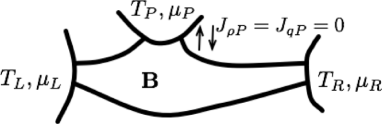
Figure 1: Schematic drawing of the model. The third (probe) reservoir introduces non-unitary noise.

The probe reservoir is adjusted in such a way that $J_{3}=J_{4}=0$, that is, the net particle and heat flow from the probe into the system vanishes. It is convenient to write Eq. (4) in the block matrix form

$$\left(\begin{array}[]{c}{\bm{J}_{\alpha}}\\ {\bm{J}_{\beta}}\end{array}\right)=\left(\begin{array}[]{cc}{\bm{L}_{\alpha\alpha}}&{\bm{L}_{\alpha\beta}}\\ {\bm{L}_{\beta\alpha}}&{\bm{L}_{\beta\beta}}\end{array}\right)\left(\begin{array}[]{c}{\bm{X}_{\alpha}}\\ {\bm{X}_{\beta}}\end{array}\right),$$ (5)

where ${\bm{\alpha}}$ stands for $(1,2)$ and ${\bm{\beta}}$ for $(3,4)$. The self-consistency condition ${\bm{J}_{\beta}}=(J_{3},J_{4})=0$ implies ${\bm{X}_{\beta}}=-{\bm{L}_{\beta\beta}}^{-1}{\bm{L}_{\beta\alpha}}{\bm{X}_{\alpha}}$, so that

$${\bm{J}_{\alpha}}={\bm{L}}^{\prime}{\bm{X}_{\alpha}},\quad{\bm{L}}^{\prime}\equiv{\bm{L}_{\alpha\alpha}}-{\bm{L}_{\alpha\beta}}{\bm{L}_{\beta\beta}}^{-1}{\bm{L}_{\beta\alpha}}.$$ (6)

The problem has then been reduced to two coupled fluxes:

$$\left(\begin{array}[]{c}J_{1}\\ J_{2}\end{array}\right)=\left(\begin{array}[]{cc}L_{11}^{\prime}&L_{12}^{\prime}\\ L_{21}^{\prime}&L_{22}^{\prime}\end{array}\right)\left(\begin{array}[]{c}X_{1}\\ X_{2}\end{array}\right),$$ (7)

where the reduced $2\times 2$ Onsager matrix matrix ${\bm{L}}^{\prime}$ fulfills the Onsager-Casimir relations

$$L_{ij}^{\prime}({\bm{B}})=L_{ji}^{\prime}(-{\bm{B}}),\quad(i,j=1,2).$$ (8)

We would like to draw the reader’s attention to the fact that the matrix ${\bm{L}}^{\prime}$ is the Onsager matrix for two-terminal noisy transport, with noise modeled by means of a self-consistent reservoir. In particular, the Seebeck and the Peltier coefficients are given by $S=L_{12}^{\prime}/(eTL_{11}^{\prime})$ and $\Pi=L_{21}^{\prime}/(eL_{11}^{\prime})$. The thermopower is asymmetric when $L_{12}^{\prime}({\bm{B}})\neq L_{21}^{\prime}({\bm{B}})$, i.e. $\Pi\neq ST$.

A key point is that, since $J_{3}=J_{4}=0$, $J_{1}$ is the charge current from left to right reservoir and the heat is extracted from (for power generation) or dissipated to (for refrigeration) the left (or right) reservoir only. Therefore, we can apply the analysis developed in Ref. ZTmag . In particular, the efficiency depends on the asymmetry parameter $x$ and on the “figure of merit” parameter $y$:

$$x=\frac{L_{12}^{\prime}}{L_{21}^{\prime}},\quad y=\frac{L_{12}^{\prime}L_{21}^{\prime}}{{\rm det}{\bm{L}}^{\prime}}.$$ (9)

For power generation ($J_{2}>0$ and output power $\omega=-J_{1}\Delta\mu=-J_{1}eTX_{1}>0$) the efficiency $\eta=\omega/J_{2}$ has a maximum value

$$\eta_{\rm max}=\eta_{C}\,x\,\frac{\sqrt{y+1}-1}{\sqrt{y+1}+1},$$ (10)

while for refrigeration ($J_{2}<0$, $\omega<0$) the maximum of the efficiency $\eta^{(r)}=J_{2}/\omega$ is

$$\eta_{\rm max}^{(r)}=\eta_{C}\,\frac{1}{x}\,\frac{\sqrt{y+1}-1}{\sqrt{y+1}+1}.$$ (11)

Non-interacting systems. Exact calculation of thermopower and efficiencies is possible for non-interacting models by means of the Landauer-Büttiker approach. We start from the bilinear Hamiltonian $H=H_{S}+H_{R}+H_{C}$, where the different terms correspond, respectively, to the nanoscale electronic system, the reservoirs, and the reservoir-system coupling. The tight-binding $N$-site system Hamiltonian reads

$$H_{S}=\sum_{n,n^{\prime}=1}^{N}H_{nn^{\prime}}c_{n}^{\dagger}c_{n}^{\prime},$$ (12)

where $c_{n}$ and $c_{n}^{\dagger}$ are fermionic annihilation and creation operators. The reservoirs are modeled as ideal fermi gases: $H_{R}=\sum_{k,q}E_{q}c_{kq}^{\dagger}c_{kq}$, where $c_{kq}^{\dagger}$ creates an electron in the state $q$ in the $k$-th reservoir. The coupling (tunneling) Hamiltonian

$$H_{C}=\sum_{k,q}(t_{kq}c_{kq}^{\dagger}c_{i_{k}}+t_{kq}^{*}c_{kq}c_{i_{k}}^{\dagger})$$ (13)

establishes the contact between site $i_{k}$ and reservoir $k$ footnote .

The charge and heat currents from the left terminal (reservoir) are given by sivan

$$J_{1}=\frac{e}{h}\int_{-\infty}^{\infty}dE\sum_{k}[T_{kL}(E)f_{L}(E)-T_{Lk}(E)f_{k}(E)],$$ (14)

$$J_{2}=\frac{1}{h}\int_{-\infty}^{\infty}dE(E-\mu_{L})\sum_{k}[T_{kL}(E)f_{L}(E)-T_{Lk}(E)f_{k}(E)],$$ (15)

where $f_{k}(E)=\{\exp[(E-\mu_{k})/k_{B}T_{k}]+1]^{-1}$ is the Fermi function and $T_{kl}$ is the transmission probability from terminal $l$ to terminal $k$. Analogous expressions can be written for $J_{3}$ and $J_{4}$, provided the terminal $L$ is substituted by $P$.

The Onsager coefficients $L_{ij}$ are obtained from the linear response expansion of the currents $J_{i}$. We have

$$L_{11}=\frac{e^{2}}{h}\int_{-\infty}^{\infty}dE\sum_{k\neq L}T_{Lk}(E)F(E),$$ (16)

$$L_{12}=L_{21}=\frac{e}{h}\int_{-\infty}^{\infty}dE(E-\mu)\sum_{k\neq L}T_{Lk}(E)F(E),$$ (17)

$$L_{22}=\frac{1}{h}\int_{-\infty}^{\infty}dE(E-\mu)^{2}\sum_{k\neq L}T_{Lk}(E)F(E),$$ (18)

where $F(E)\equiv-Tf^{\prime}(E)=1/4k_{B}\cosh^{2}[(E-\mu)/k_{B}T]$. Analogous formulas are obtained for $L_{33}$, $L_{34}=L_{43}$, and $L_{44}$, with the $P$ terminal used instead of $L$. Note that for the non-interacting three-teminal model $L_{12}$ is still an even function of the magnetic field, that is, $L_{12}=L_{21}$. On the other hand the symmetry of the off-diagonal matrix elements is broken for the reduced Onsager matrix ${\bm{L}}^{\prime}$. Indeed, reduction (6) involves other off-diagonal matrix elements of ${\bm{L}}$ – between ‘left’ $(1,2)$ and ‘probe’ $(3,4)$ sectors – which in general are not even functions of an applied magnetic field. The block ${\bm{L}_{\alpha\beta}}$ of matrix ${\bm{L}}$ is given by

$${\bm{L}_{\alpha\beta}}=-\frac{e^{2}}{h}\int_{-\infty}^{\infty}dE\left(\begin{array}[]{cc}1&\frac{E-\mu}{e}\\ \frac{E-\mu}{e}&\left(\frac{E-\mu}{e}\right)^{2}\end{array}\right)T_{LP}(E)F(E),$$ (19)

and ${\bm{L}_{\alpha\beta}}\neq{\bm{L}_{\beta\alpha}}$, since ${\bm{L}_{\beta\alpha}}$ is obtained from ${\bm{L}_{\alpha\beta}}$ after substitution of $T_{LP}$ with $T_{PL}$ and in general $T_{LP}\neq T_{PL}$.

The transmission probabilities are given by datta

$$T_{pq}={\rm Tr}[\Gamma_{p}(E)G(E)\Gamma_{q}(E)G^{\dagger}(E)],$$ (20)

where the broadening matrices $\Gamma_{k}$ are defined in terms of the self-energies $\Sigma_{k}$: $\Gamma_{k}(E)\equiv i[\Sigma_{k}(E)-\Sigma_{k}^{\dagger}(E)]$ and the (retarded) system Green function $G(E)\equiv[E-H_{S}-\sum_{k}\Sigma_{k}(E)]^{-1}$.

Aharonov-Bohm interferometer. As an illustrative, realistic example we consider a three-dot ring structure pierced by an Aharonov-Bohm flux, with dot $k$ coupled to reservoir $k$, as sketched in Fig. 2. The system Hamiltonian reads

$$\begin{array}[]{c}H_{S}=\sum_{k}\epsilon_{k}c_{k}^{\dagger}c_{k}+\\ \\ (t_{LR}c_{R}^{\dagger}c_{L}e^{i\phi/3}+t_{RP}c_{P}^{\dagger}c_{R}e^{i\phi/3}+t_{PL}c_{L}^{\dagger}c_{P}e^{i\phi/3}+\hbox{H.c.}),\end{array}$$ (21)

and the broadening matrices are $\Gamma_{k}=\gamma_{k}c_{k}^{\dagger}c_{k}$. We apply the Landauer-Büttiker approach to this model, numerically computing the Onsager coefficients following Eqs. (16)-(20).

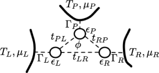
Figure 2: Schematic drawing of the three-dot model.

As expected, we obtain asymmetric off-diagonal reduced Onsager matrix elements, that is $L_{12}^{\prime}\neq L_{21}^{\prime}$, as far as the Aharonov-Bohm flux $\phi$ is non-vanishing and there is anisotropy in the systems, for instance when $\epsilon_{L}\neq\epsilon_{R}$. Since the thermopower is not symmetric with respect to the magnetic field, i.e. $L_{12}^{\prime}({\bm{B}})\neq L_{12}^{\prime}(-{\bm{B}})=L_{21}^{\prime}({\bm{B}})$, then in general the ratio $x=L_{12}^{\prime}/L_{21}^{\prime}\neq 1$. The asymmetry parameter $x$ can be made arbitrarily small when $L_{21}^{\prime}\to 0$ or arbitrarily large when $L_{21}^{\prime}\to 0$, see for instance Fig. 3.

Figure 3: Ratio $x$ of the off-diagonal matrix elements $L_{12}^{\prime}$ and $L_{21}^{\prime}$ of the reduced Onsager matrix at $T=1$, $\mu=0.3$, $\epsilon_{L}=0$, $\epsilon_{R}=0.5$, $\epsilon_{P}=1$, all hopping terms $t_{pq}=-1$, broadenings $\gamma_{k}=0.1$ independently of energy (wide-band limit). Hereafter we set $e=\hbar=k_{B}=1$.

Remarks. Large asymmetries ipso facto do not imply large efficiencies. For example, in the case of Fig. 3 when $x$ diverges the figure of merit $y$ and the efficiency tend to zero. It is however interesting to compare the efficiencies of power generation and refrigeration. While in the time-symmetric case the two efficiencies coincide, $\eta_{\rm max}(\phi=0)=\eta_{\rm max}^{(r)}(\phi=0)$, this is no longer the case when $x\neq 1$. For small fields $x$ is in general a linear function of the field, $x(\phi)=1+\alpha\phi+O(\phi^{2})$, while $y$ is by construction an even function of the field, so that $y(\phi)=y(0)+\beta\phi^{2}+O(\phi^{4})$. From Eqs. (10) and (11) we obtain $\eta_{\rm max}(\phi)=\eta_{\rm max}(0)[1+\alpha\phi+O(\phi^{2}))]$ and $\eta_{\rm max}^{(r)}(\phi)=\eta_{\rm max}(0)[1-\alpha\phi+O(\phi^{2}))]$. Therefore, a small external magnetic field either improves power generation and worsens refrigeration or vice-versa, while the average efficiency $\bar{\eta}\equiv[\eta_{\rm max}(\phi)+\eta_{\rm max}^{(r)}(\phi)]/2=\eta_{\rm max}(0)$ up to second order corrections. Due to the Onsager-Casimir relations $x(-\phi)=1/x(\phi)$ and therefore by inverting the direction of the magnetic field one can improve either power generation or refrigeration.

In conclusion, we have shown that non-unitary noise generally leads to a thermopower which is a non-symmetric function of the magnetic field. Such general result has been illustrated by means of a realistic three-dot Aharonov-Bohm interferometer model, which appears suitable for experimental investigations by means of three-terminal mesoscopic devices. The asymmetry of the Seebeck coefficient with respect to the magnetic field allows in principle, in the linear response regime, to obtain a finite power at Carnot efficiency. Whether this is actually the case remains an interesting open problem. An additional interesting open problem is whether noiseless interacting systems might exhibit asymmetric thermopower.

KS was supported by MEXT, Grant Number (23740289), GB and GC by the MIUR-PRIN 2008 and by Regione Lombardia, and TP by the Grants J1-2208 and P1-0044 of Slovenian Research Agency.

References

- (1) G. Benenti, K. Saito, and G. Casati, Phys. Rev. Lett. 106, 230602 (2011).
- (2) S. Datta, Electronic Transport in Mesoscopic Systems (Cambridge University Press, 1995).
- (3) S.A. van Langen, P.G. Silvestrov, and C.W.J. Beenakker, Superlattices Microstruct. 23, 691 (1998); S.F. Godijn, S. Moller, H. Buhmann, L.W. Molenkamp, and S.A. van Langen, Phys. Rev. Lett. 82, 2927 (1999).
- (4) J. Eom, C.-J. Chien, and V. Chandrasekhar, Phys. Rev. Lett. 81, 437 (1998).
- (5) Ph. Jacquod and R.S. Whitney, Europhys. Lett. 91, 67009 (2010).
- (6) O. Entin-Wohlman, Y. Imry, and A. Aharony, preprint.
- (7) C. Mejía-Monasterio, private communication.
- (8) M. Büttiker, IBM J. Res. Developm. 32, 63 (1988).
- (9) To simplify writing we have considered spinless fermions; however, the model can be readily extended to include the spin degrees of freedom.
- (10) U. Sivan and Y. Imry, Phys. Rev. B 33, 551 (1986); P.N. Butcher, J. Phys.: Condens. Matter 2, 4869 (1990).
- (11) H.B. Callen, Thermodynamics and an Introduction to Thermostatics (second edition) (John Wiley & Sons, New York, 1985).