Footprint traversal by ATP-dependent chromatin remodeler motor

Abstract

ATP-dependent chromatin remodeling enzymes (CRE) are bio-molecular motors in eukaryotic cells. These are driven by a chemical fuel, namely, adenosine triphosphate (ATP). CREs actively participate in many cellular processes that require accessibility of specific segments of DNA which are packaged as chromatin. The basic unit of chromatin is a nucleosome where 146 bp $\sim$ 50 nm of a double stranded DNA (dsDNA) is wrapped around a spool formed by histone proteins. The helical path of histone-DNA contact on a nucleosome is also called “footprint”. We investigate the mechanism of footprint traversal by a CRE that translocates along the dsDNA. Our two-state model of a CRE captures effectively two distinct chemical (or conformational) states in the mechano-chemical cycle of each ATP-dependent CRE. We calculate the mean time of traversal. Our predictions on the ATP-dependence of the mean traversal time can be tested by carrying out in-vitro experiments on mono-nucleosomes.

I Introduction

A deoxyribonucleic acid (DNA) molecule is a linear heteropolymer whose monomeric subunits, called nucleotides, are denoted by the four letters A, T, C and G. The sequence of these nucleotides in a DNA molecule chemically encodes genetic informations. In the nucleus of an eukaryotic cell, DNA is stored in a hierarchically organized structure called chromatin wolffe98 ; widom98 ; schiessel03 ; lavelle06 . The primary repeating unit of chromatin at the lowest level of the hierarchical structure is a nucleosome kornberg99 . The cylindrically shaped core of each nucleosome consists of an octamer of histone proteins around which 146 base pairs (i.e.,$\sim 50$ nm) of the the double stranded DNA is wrapped about two turns (more precisely, 1.7 helical turns); the arrangement is reminiscent of wrapping of a thread around a spool. There are $14$ equispaced sites, at intervals of $10$ base pairs (bp), on the surface of the cylindrical spool. Electrostatic attraction between these binding sites on the histone spool and the oppositely charged DNA seems to dominate the histone-DNA interactions which stabilize the nucleosomes. Throughout this paper, the helical curve formed by the histone-DNA overlap will be called the “footprint”.

The DNA stores the genetic blueprint of an organism. If nucleosomes were static, segments of DNA buried in nucleosomes would not be accessible for various functions involving the corresponding gene polach95 ; anderson02 ; fan03 . However, in reality, nucleosomes are dynamic. Spontaneous dynamics of nucleosomes are usually consequences of thermal fluctuations whereas the active dynamic processes are driven by special purpose molecular machines called chromatin remodeling enzymes (CRE) fuelled by ATP flaus03 ; flaus11 ; halford04a ; saha06 ; clapier09 ; narlikar08 . Various aspects of chromatin dynamics has received some attention of theoretical modelers, including physicists, over the last few years sakaue01 ; schiessel01 ; kulic03a ; kulic03b ; schiessel06 ; rafiee04 ; blossey11 ; mobius06 ; langowski06 ; lense06 ; vaillant06 ; ranjith07 ; lia06 .

In general, “Chromatin remodelling” refers to a range of enzyme mediated structural transitions that occur during gene regulation in eukaryotic cells. To make DNA, which is wrapped around histone octamer, accessible for various DNA-dependent processes, it is always necessary to rearrange or mobilize the nucleosomes. In principle, there are at least four different ways in which a CRE can affect the nucleosomes cairns07 : (i) sliding the histone octamer, i.e., repositioning of the entire histone spool, on the dsDNA; (ii) exchange of one or more of the histone subunits of the spool with those in the surrounding solution (also called replacement of histones) (iii) removal of one or more of the histone subunits of the spool, leaving the remaining subunits intact, and (iv) complete ejection of the whole histone octamer without replacement. Our theoretical work here is closely related to sliding.

In the next section we describe a scenario in which either a CRE motor (or, other ATP-dependent motors that translocate along dsDNA) traverse the “footprint”. Because of the stochasticity of the underlying mechano-chemical kinetics, the footprint traversal time (FTT) is a fluctuating random variable. Extending an earlier model developed by Chou chou , we analytically calculate the mean FTT (MFTT) of the CRE motor.

To our surprise, we found that the ATP-dependence of the various ATP-driven activities of CREs have not been studied systematically in the published literature. In particular, we address the question: how does the MFTT of a CRE motor vary with the variation of the concentration of ATP? This rate is not necessarily directly proportional to the rate of ATP hydrolysis by the CRE because the mechanical sliding of the nucleosome need not be tightly coupled with the hydrolysis of ATP by the CRE. Therefore, we develope here an analytical theory predicting the ATP-dependence of the ATP-dependent footprint-traversal by CRE. We hope our result will stimulate systematic experimental investigations on the ATP-dependence of ATP-dependent CREs.

II CRE: phenomenology and motivation for this work

Chromatin is not a frozen static aggregate of DNA and proteins. Spontaneous thermal fluctuations can cause a transient unwrapping and rewrapping of the nucleosomal DNA from one end of the nucleosome spool; the corresponding rates for an isolated single nucleosome are, typically, $4$s^-1 and $20-90$s^-1, respectively li04 . In other words, once wrapped fully, the nucleosomal DNA remains in that state for about $250$ms before unwrapping again spontaneously; however, it waits in the unwrapped state only for about $10-50$ms before rewrapping again spontaneously. Surprisingly, the accessibility of the nucleosomal DNA is only modestly affected if instead of a single nucleosome the experiment is repeated with an array of homogeneously distributed nucleosomes poirier08 ; poirier09 . Moreover, folding of an array of nucleosomes makes the linker DNA about $50$ times less accessible poirier08 ; poirier09 . Furthermore, on the nucleosomal DNA, the farther is a site from the entry and exit points, the longer one has to wait to access it by the rarer spontaneous fluctuation of sufficiently large size tims11 . Thus, nucleosomal DNA far from both the entry and exit sites is practically inaccessible by spontaneous thermal fluctuations.

Can a nucleosome slide spontaneously by thermal fluctuations thereby exposing the nucleosomal DNA? Interestingly, spontaneous repositioning of nucleosome on DNA strands is a well known phenomenon meerssman92 . How can one reconcile accessibility of nucleosomal DNA by such repositioning meerssman92 with the difficulty of access by unwrapping from either end of the spool tims11 ? If the DNA were to move unidirectionally along its own superhelical contour on the surface of the histone, at every step it would have to first transiently detach simultaneously from all the $14$ binding sites and then reattach at the same sites after its contour gets shifted by $10$ bp (or multiples of $10$ bp). But, the energy cost of the simultaneous detachment of the DNA from all the $14$ binding sites is prohibitively large because the total energy of binding at the $14$ sites is about $75k_{B}T$ blossey11 ; kulic03a ; kulic03b .

But, why can’t the cylindrical spool simply roll on the wrapped nucleosomal DNA thereby repositioning itself? If the nucleosome rolls by detaching DNA from one end of the spool, cannot it compensate this loss of binding energy by simulataneous attachment with a binding at the other end? If such an energy compensation were possible, detachment from only one binding site would be required at a time. But, the cylindrical spool has a finite size on which only a finite number ($14$) of binding sites for DNA are accomodated. Therefore, by rolling over the DNA the spool would not offer any vacant binding site to the DNA with which it can bind. This rolling mechanism would successfully lead to spontaneous sliding of the nucleosome only if the histone spool were infinite with an infinite sequence of binding sites for DNA on its surface blossey11 .

We now describe a plausible mechanism for spontaneous sliding of a nucleosome schiessel01 ; kulic03a ; kulic03b . In the process of normal “breathing”, most often the spontaneously unwrapped flap rewraps exactly to its original position on the histone surface. However, if the rewrapping of a unwrapped flap takes place at a slightly displaced location on the histone spool a small bulge (or loop) of DNA forms on the surface of the histones. Since the successive binding sites are separated by $10$bp, the length of the loop is quantized in the multiples of $10$bp schiessel01 . Such a spontaneously created DNA loop, can diffuse in an unbiased manner on the surface of the histone spool. In the beginning of each step DNA from one end of the loop detaches from the histone spool, but the consequent energy loss is made up by the attachment of DNA at the other end of the loop to the histone spool before the step is completed. Consequently, by this diffusive dynamics, the DNA loop can traverse the entire length of the $14$ binding sites on the histone spool of a nucleosome which will manifest as sliding of the nucleosome by a length that is exactly equal to the length of DNA in the loop. The diffusing DNA bulge can be formed by a “twist”, rather than bending, of DNA lusser03 ; becker02a ; langst04 . Spontaneous sliding of a nucleosome, however, is too slow to support intranuclear processes which need access to nucleosomal DNA.

It is now widely agreed that ATP-dependent active remodeling of nucleosome can account for the fast sliding of nucleosomes. Nevertheless, bulging DNA loop is expected to play a key role in the remodeling process lia06 . Our model describes how a CRE motor can wedge itself at the fork between the histone spool and a transiently detached segment of dsDNA and, by exploiting the spontaneously diffusing loop by an ATP-dependent ratcheting, traverse the footprint in a directed manner. Because of the intrinsic stochasticity of the mechano-chemistry of the CRE and that of the diffusive motion of the DNA loop, the overall motion of the CRE is noisy and the time it takes to traverse the footprint is random.

The main question we address in this paper is the following: if $<T>$ is the MFTT, what is the dependence of $<T>$ on the concentration of ATP in the surrounding aqueous medium? To our knowledge, in the published literature neither systematic experiments nor any analytical theory has addressed this question. In this paper, by extending Chou’s model chou of CRE, we capture the role of ATP explicitly and derive an analytical expression for the dependence of $<T>$ on the concentration of ATP.

A CRE may be regarded as a molecular motor where input energy is derived from ATP hydrolysis and the output is mechanical work. The directed movement of the CRE may be caused either by a power stroke or by a Brownian ratchet mechanism widom98 . The kinetics of the ATP-dependent CRE motor is formulated in our model in terms of a set of master equations. The kinetic scheme can be interpreted in terms of both power stroke and Brownian ratchet mechanisms.

One interesting question cairns07 in the context of CRE is whether the CRE translocates along the DNA by moving around the nucleosome, or whether the CRE anchors on the histone octamer and “pumps” DNA by pulling around the octamer. From the perspective of physicists, these two alternative scenarios can be viewed as merely a change of frame of reference- one is fixed with respect to the DNA whereas the other is fixed with respect to the CRE. Therefore, we describe the operation of the CRE with respect to a reference frame with respect to which the CRE translocates along the DNA; but, the model can be reformulated by a coordinate transformation so as to capture the alternative scenario where the CRE pumps the DNA.

III The Model

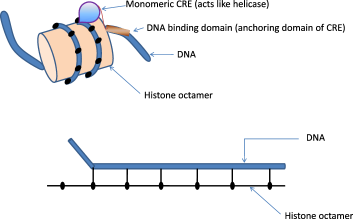
Figure 1: A schematic representation of the isolated nucleosome.

We model a mono nucleosome where a dsDNA is wrapped one-and-three-fourth turn around a disc-shaped spool made of histone proteins (see Fig.1(a)). Following Chou chou , we consider the scenario where the CRE “wedges itself underneath the histone”.

The sites of histone-DNA contact along the DNA chain is represented as a one-dimensional lattice. Therefore, the lattice constant is, typically, $10$ bp ((see Fig.1(b)). The total number $n$ of lattice sites is equal to the total number of histone-DNA contact in a single nucleosome.

III.1 Flap, loop and diffusive sliding of histone spool

In this subsection we present a summary of Chou’s ideas chou which we need in the next subsection where we extend Chou’s model. Here we consider the simple situation when no CRE is present and the kinetics of the system is governed solely by spontaneous thermal fluctuations. Because of these fluctuations, from either end of the histone-DNA contact region, small segments of DNA momentarily unwrap from the histone spool at a rate $k_{u}$. For energetic reasons, the most likely length of such a segment would be one lattice spacing, i.e., about $10$bp. Following Chou chou , we call such unwrapped segments a “flap”. The rate of the reverse transition, in which re-binding of the DNA flap with the histone, takes place at a rate $k_{b}$.

A flap need not re-make the original histone-DNA contact. Instead, by pulling in an extra segment of the DNA, its next segment can bind with the last binding site on the histone spool, with rate $\alpha$ thereby forming what Chou chou referred to as a “loop’. While located at either end of the lattice, a loop can revert to a flap at a rate $\beta$. The rates $\alpha$ and $\beta$ are well approximated by chou

$$\alpha\sim k_{b}e^{-E_{bend}/(k_{B}T)},~{}{\rm and}~{}\beta\sim k_{u}$$ (1)

where $E_{bend}$ is the energy cost of bending the DNA into the shape of the loop.

Figure 2: A schematic representation of the position of the thermally generated flap and it’s diffusion along wrapped DNA.

A loop can step forward or backward. In the absence of any CRE, the rates of the forward and backward steppings of the loop are equal (denoted by $k$), provided the size of the loop $L_{loop}$ remains unaltered (see Fig.2); in each forward step it unwraps one segment of DNA from the histone in the direction of its hop and re-wraps another equally long segment behind it. Therefore, one can approximate $k$ by chou

$$k\sim k_{u}\biggl{(}\frac{k_{b}}{(k_{b}+k_{u})}\biggr{)}$$ (2)

When a loop, after entering the lattice from one end, makes an eventual exit from the other end, it completes the “sliding” of the histone spool by a distance $L_{loop}$ along the DNA in the opposite direction. Therefore, from the perspective of the sliding histone spool, its effective rate of hopping by a step of size $L_{loop}$ along the dsDNA strand is the same as the rate $p_{n}$ at which a DNA loop of length $L_{loop}$ traverses the lattice of $n$ sites from one end to the other.

Suppose ${\cal P}_{j}(t)$ denotes the probability that the loop is located at $j$ ($0\leq j\leq 1$). Following Chou’s arguments, based on master equations for ${\cal P}_{j}(t)$, one gets chou

$$p_{n} = \frac{\alpha kk_{u}}{(n-1)\beta k_{b}+k(\alpha+2k_{b})}$$ (3)

In the absence of a CRE, the traversal of a DNA loop of length $L_{loop}$ from left to right is as likely as that from right to left. Therefore, the histone spool can slide forward or backward, with equal rate $p_{n}$, by a step of size $L_{loop}$. As we’ll see in the next subsection, peeling off of the DNA from the histone spool by a CRE motor keeps decreasing the effective value of $n$ which, in turn, increases the effective sliding rate $p_{n}$.

III.2 Kinetics of CRE-driven directed sliding of histone spool

Next, we consider the effect of DNA loop diffusion on the ATP-dependent translocation kinetics of a CRE. The model and results presented in this subsection are extensions of Chou’s work chou by incorporating explicitly a Brownian ratchet mechanism for CRE motors.

As in ref.chou , we assume that the step size of the CRE motor is identical to the length of the thermally generated DNA loop. Therefore, the mechanical movements of the CRE motor can be described as that of a “particle” on the one-dimensional lattice on which the equi-spaced sites denote the histone-DNA contact points. We denote the position of the CRE motor on this lattice by the integers $m$. We now extend Chou’s model chou by exploiting a superficial similarity with the Garai-Chowdhury-Betterton (GCB) model garai for the Brownian ratchet mechanism of monomeric helicase motors.

A DNA helicase unwinds a dsDNA and translocates along one of two strands. At any arbitrary instant of time, the configuration of the system looks very similar to that shown in Fig.1(b) except that the surface of the DNA spool and the dsDNA would be replaced by the two strands of the dsDNA itself. The lattice constant is $1$bp in the case of a helicase whereas it is about $10$ bp in Fig.1(b). In the Brownian ratchet mechanism, momentary local unwinding of a segment, typically, $1$ bp long, takes place at the fork by spontaneous thermal fluctuation; the opportunistic advance of the helicase merely prevents closure of the segment. Similarly, in the Brownian ratchet mechanism of the CRE, the CRE is assumed to “wedge” itself just in front of the DNA-histone fork. The CRE motor can move forward only if the segment in front of it is unwrapped by thermal fluctuation.

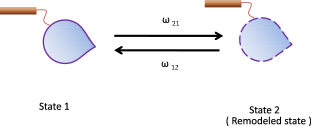
Figure 3: A schematic representation of the transition of the CRE between its two states.

The mechano-chemical cycle of the CRE is captured in our model exactly the same way in which that of the helicase was formulated in the GCB model garai . We assume that sequence of states in each mechano-chemical cycle of a CRE can be combined into two distinct groups which we label by the integers $1$ and $2$ (see Fig.3). The allowed transitions and the corresponding rate constants are shown in Fig.4.

Figure 4: A schematic representation of the position of the motor with two state of the model.

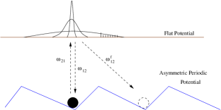
Figure 5: A schematic representation of the Brownian ratchet mechanism.

The physical processes captured by these rate constants can be motivated by a comparison with the abstract Brownian ratchet mechanism, illustrated in Fig.5. ATP hydrolysis by the CRE drives its transition from the state $1$ to the state $2$ at a rate $\omega_{21}$. Let us assume that the motor experiences two different types of potentials in the states $1$ and $2$. Let us further assume that initially the periodic potential, with asymmetric sawtooth-like period, is kept on for sometime and during this time the motor settles at a position that coincides with one of the minima of this potential. Now if this potential is switched off then the probability distribution of the position of the motor will spread as a symmetric Gaussian. After sometime this Gaussian profile is broad enough to overlap with the next well (shadded region in the Fig.5), in addition to the original well. Now if the sawtooth potential is again switched on then, with a non-zero probability (that is proportional to the area of the shaded region) the motor will find itself in the next well. Our model accounts for this possibility with the transition associated with the rate constant $\omega^{f}_{12}$. There is also a finite probability that the particle stays back in its original well; this is captured by the transition with the rate constant $\omega_{12}$.

The CRE motor would step forward at the rate $\omega^{f}_{12}$ if the next site in front is cleared. But if the next site is not cleared and it has to wait for the unwrapping of the DNA segment by thermal fluctuation. Consequently, its effective hoping rate

$$\tilde{\omega}^{f}_{12}=k_{u}\biggl{(}\frac{\omega^{f}_{12}}{(\omega^{f}_{12}+k_{b})}\biggr{)}$$ (4)

is reduced from the free hopping rate $\omega^{f}_{12}$ by a factor that depends on both $k_{u}$ and $k_{b}$.

When a diffusing loop reaches in front of the motor it momentarily creates a flap of two bond segments. Three different transitions are now possible (see Fig.6): (i) the motor’s position remains unaltered while the two open segments close, (ii) the motor moves forward by one step while one segment of the flap closes; (iii) the motor moves forward by two steps and the flap cannot close. The rate for the process (i) is $k_{b}/2$ irrespective of the “chemical” state of the motor. However, the rates of the processes (ii) and (iii) depend on whether the motor was in the “chemical” state $1$ or $2$. If the motor is in the state $2$, the rate of the process (ii) is given by $((\omega^{f}_{12})^{-1}+k_{b}^{-1})^{-1}$ and that of the process (iii) is given by $((\omega^{f}_{12})^{-1}+(\omega_{21})^{-1}+(\omega^{f}_{12})^{-1})$. Therefore,

$$f_{0} = \frac{k_{b}}{2\lambda_{f}},f_{1}=\frac{\omega^{f}_{12}k_{b}}{(\omega^{f}_{12}+k_{b})\lambda_{f}},f_{2}=\frac{\omega^{f}_{12}\omega_{21}}{\lambda_{f}(2\omega_{21}+\omega^{f}_{12})},$$ (5)

with the normalization constant

$$\lambda_{f}=\frac{k_{b}}{2}+\frac{\omega^{f}_{12}k_{b}}{(\omega^{f}_{12}+k_{b})}+\frac{\omega^{f}_{12}\omega_{21}}{(2\omega_{21}+\omega^{f}_{12})}$$ (6)

where the symbols $f_{0}$, $f_{1}$ and $f_{2}$ are the probabilities of the processes (i), (ii) and (iii) above when the motor is in the “chemical” state $2$. Similarly,

$$g_{0} = \frac{k_{b}}{2\lambda_{h}},g_{1}=\frac{k_{b}\omega_{21}\omega^{f}_{12}}{(\omega_{21}\omega^{f}_{12}+k_{b}\omega^{f}_{12}+k_{b}\omega_{21})\lambda_{h}},$$

$$g_{2} = \frac{\omega_{21}\omega^{f}_{12}}{2(\omega^{f}_{12}+\omega_{21})\lambda_{h}},$$ (7)

with the normalization constant

$$\lambda_{h} = \frac{k_{b}}{2}+\frac{k_{b}\omega_{21}\omega^{f}_{12}}{\omega_{21}\omega^{f}_{12}+k_{b}\omega^{f}_{12}+k_{b}\omega_{21}}$$ (8)

$$+ \frac{\omega_{21}\omega^{f}_{12}}{2(\omega^{f}_{12}+\omega_{21})},$$

are the corresponding probabilities, when the motor is in the “chemical” state $1$.

(a)

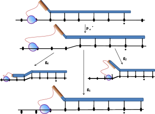
(b)

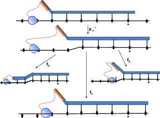
Figure 6: Schematic representations of the possible transitions when the motor is in front of the open flap. In (a) and (b) the motor is in the chemical state $1$ and $2$, respectively.

Suppose, $N$ is the maximum number of histone-DNA contacts possible in the nucleosome. Let $m$ denote the instantaneous position of the motor. $n$ is the distance between the motor and the far end of histone-DNA contact. The master equations for the probabilities $P(m,n,t)$ are as follows:

For n$\geq$N+1

$$dP_{1}(m,n)/dt = \omega_{12}P_{2}(m,n)-\omega_{21}P_{1}(m,n)$$ (9)

$$+ \omega^{f}_{12}P_{2}(m-1,n+1)$$

$$+ p_{N}[P_{1}(m,n+1)+P_{1}(m,n-1)$$

$$~{}~{}~{}~{}-2P_{1}(m,n)]$$

and

$$dP_{2}(m,n)/dt = \omega_{21}P_{1}(m,n)-\omega_{12}P_{2}(m,n)$$ (10)

$$- \omega^{f}_{12}P_{2}(m,n)$$

$$+ p_{N}[P_{2}(m,n+1)+P_{2}(m,n-1)$$

$$~{}~{}~{}~{}-2P_{2}(m,n)]$$

For n=N

$$dP_{1}(m,N)/dt = \omega_{12}P_{2}(m,N)-\omega_{21}P_{1}(m,N)$$ (11)

$$+ \omega^{f}_{12}P_{2}(m-1,N+1)$$

$$+ p_{N}[P_{1}(m,N+1)-P_{1}(m,N)]$$

$$+ p_{N}[f_{1}P_{2}(m-1,N)$$

$$~{}~{}~{}~{}+g_{1}P_{1}(m-1,N)]$$

$$+ p_{N-1}g_{0}P_{1}(m,N-1)$$

and

$$dP_{2}(m,N)/dt = \omega_{21}P_{1}(m,N)-\omega_{12}P_{2}(m,N)$$ (12)

$$- \tilde{\omega}^{f}_{12}P_{2}(m,N)$$

$$+ p_{N}[P_{2}(m,N+1)-P_{2}(m,N)]$$

$$+ f_{0}p_{N-1}P_{2}(m,N-1)$$

For 3$\leq$ n $\leq$ N

$$dP_{1}(m,n)/dt = \omega_{12}P_{2}(m,n)-\omega_{21}P_{1}(m,n)$$ (13)

$$+ \tilde{\omega}^{f}_{12}P_{2}(m-1,n+1)-p_{n}P_{1}(m,n)$$

$$+ p_{n}[f_{1}P_{2}(m-1,n)+g_{1}P_{1}(m-1,n)]$$

$$+ p_{n+1}[f_{2}P_{2}(m-2,n+1)$$

$$~{}~{}~{}+g_{2}P_{1}(m-2,n+1)]$$

$$+ g_{0}p_{n-1}P_{1}(m,n-1)$$

and

$$dP_{2}(m,n)/dt = \omega_{21}P_{1}(m,n)-\omega_{12}P_{2}(m,n)$$ (14)

$$- (\tilde{\omega}^{f}_{12}+p_{N})P_{2}(m,n)$$

$$+ f_{0}p_{n-1}P_{2}(m,n-1)$$

For n$=$2

$$dP_{1}(m,2)/dt = \omega_{12}P_{2}(m,2)-\omega_{21}P_{1}(m,2)$$

$$+ \tilde{\omega}^{f}_{12}P_{2}(m-1,3)-p_{2}P_{1}(m,2)$$

$$+ p_{2}[g_{1}P_{1}(m-1,2)+f_{1}P_{2}(m-1,2)]$$

$$+ p_{3}[g_{2}P_{1}(m-2,3)+f_{2}P_{2}(m-2,3)]$$

(15)

and

$$dP_{2}(m,2)/dt = \omega_{21}P_{1}(m,2)-\omega_{12}P_{2}(m,2)$$

$$- \tilde{\omega}^{f}_{12}P_{2}(m,2)-p_{2}P_{2}(m,2)$$

For n$=$1

$$dP_{1}(m,1)/dt = \omega_{12}P_{2}(m,1)-\omega_{21}P_{1}(m,1)$$

$$+ \tilde{\omega}^{f}_{12}P_{2}(m-1,2)-k_{u}P_{1}(m,1)$$

$$+ p_{2}[f_{2}P_{2}(m-2,2)+g_{2}P_{1}(m-2,2)]$$

and

$$dP_{2}(m,1)/dt=\omega_{21}P_{1}(m,1)-\omega_{12}P_{2}(m,1)-k_{u}P_{2}(m,1)$$

(18)

Figure 7: A schematic representation of the position of the DNA-histone contact with two state of the model.

III.3 Footprint traversal time

We define $P_{\mu,n}(t)=\sum_{m}P_{\mu}(m,n,t)$ as the probability that the $n$ histone-DNA contacts are intact at time $t$, irrespective of the position of the CRE motor. From equations (9)-(18), summing over $m$, we get the following equations: For n$\geq$(N+1)

$$dP_{1,n}/dt = p_{N}[P_{1,n+1}-2P_{1,n}+P_{1,n-1}]+$$ (19)

$$\omega^{f}_{12}P_{2,n+1}+\omega_{12}P_{2,n}-\omega_{21}P_{1,n}$$

and

$$dP_{2,n}/dt = p_{N}[P_{2,n+1}-2P_{2,n}+P_{2,n-1}]+$$ (20)

$$\omega_{21}P_{1,n}-\omega_{12}P_{2,n}-\omega^{f}_{12}P_{2,n}$$

For n=N

$$dP_{1,N}/dt = -p_{N}P_{1,N}+\omega_{12}P_{2,N}+\omega^{f}_{12}P_{2,N+1}$$ (21)

$$+g_{0}p_{N-1}P_{1,N-1}+g_{1}p_{N}P_{1,N}+p_{N}$$

$$P_{1,N+1}+f_{1}p_{N}P_{2,N}-\omega_{21}P_{1,N}$$

and

$$dP_{2,N}/dt = -(\tilde{\omega}^{f}_{12}+p_{N})P_{2,N}+\omega_{21}P_{1,N}-\omega_{12}P_{2,N}$$ (22)

$$+p_{N}P_{2,N+1}+f_{0}p_{N-1}P_{2,N-1}$$

For 3$\leq$ n $\leq$ N

$$dP_{1,n}/dt = -p_{n}P_{1,n}+\tilde{\omega}^{f}_{12}P_{2,n+1}$$ (23)

$$+\omega_{12}P_{2,n}-\omega_{21}P_{1,n}+g_{0}p_{n-1}P_{1,n-1}+$$

$$g_{1}p_{n}P_{1,n}+g_{2}p_{n+1}P_{1,n+1}+f_{1}p_{n}P_{2,n}+$$

$$f_{2}p_{n+1}P_{2,n+1}$$

and

$$dP_{2,n}/dt = -(\tilde{\omega}^{f}_{12}+p_{N})P_{2,n}+\omega_{21}P_{1,n}$$ (24)

$$-\omega_{12}P_{2,n}+f_{0}p_{n-1}P_{2,n-1}$$

For n$=$1

$$dP_{1,1}/dt = -k_{u}P_{1,1}+\tilde{\omega}^{f}_{12}P_{2,2}+$$ (25)

$$f_{2}p_{2}P_{2,2}+g_{2}p_{2}P_{1,2}+\omega_{12}P_{2,1}-$$

$$\omega_{21}P_{1,1}$$

and

$$dP_{2,1}/dt=-k_{u}P_{2,1}+\omega_{21}P_{1,1}-\omega_{12}P_{2,1}$$ (26)

For n$=$2

$$dP_{1,2}/dt = -p_{2}P_{1,2}+\tilde{\omega}^{f}_{12}P_{2,3}$$ (27)

$$+g_{1}p_{2}P_{1,2}+f_{1}p_{2}P_{2,2}+g_{2}p_{3}P_{1,3}$$

$$+f_{2}p_{3}P_{2,3}+\omega_{12}P_{2,2}-\omega_{21}P_{1,2}$$

and

$$dP_{2,2}/dt = -\omega_{12}P_{2,2}+\omega_{21}P_{1,2}-p_{2}P_{2,2}$$ (28)

$$-\tilde{\omega}^{f}_{12}P_{2,2}$$

We define the survival probability $S_{\mu,n}(t)$ to be the probability that the CRE has not yet reached the far end of the footprint till time $t$, given that initially (at $t=0$) there were $n$ intact contacts between the histone spool and the DNA on the footprint in front of the CRE motor. Obviously, $S_{\mu,n}(t)$ is the solution of the equations for $P_{\mu,n}(t)$ with the initial condition $S_{\mu,n}(0)=1$.

Interestingly, the time-evolution of $S_{\mu,n}(t)$ can be re-cast as

$$dS_{1,n}/dt = a_{n}^{+}(S_{1,n+1}-S_{1,n})+a_{n}^{-}(S_{1,n-1}-S_{1,n})$$ (29)

$$+r_{n}(S_{2,n}-S_{1,n})$$

$$dS_{2,n}/dt = b_{n}^{+}(S_{2,n+1}-S_{2,n})+b_{n}^{-}(S_{2,n-1}-S_{2,n})$$ (30)

$$+s_{n}(S_{1,n}-S_{2,n})+F_{n}(S_{1,n-1}-S_{2,n})$$

where the transition rates $a^{\pm}_{n},b^{\pm}_{n},r_{n},s_{n}$ and $F_{n}$ depend on the value of $n$ as follows: For $n\geq(N+1)$

$F_{n}=\omega^{f}_{12},a_{n}^{+}=p_{N},a_{n}^{-}=p_{N},b_{n}^{+}=p_{N},b_{n}^{-}=p_{N},r_{n}=\omega_{21},s_{n}=\omega_{12}$

For n=N

$F_{n}=\omega^{f}_{12},a_{n}^{+}=g_{0}p_{N},a_{n}^{-}=p_{N},b_{n}^{+}=f_{0}p_{N},b_{n}^{-}=p_{N},r_{n}=\omega_{21},s_{n}=(\omega_{12}+f_{1}p_{N})$

For $3\leq n<N$

$F_{n}=(\tilde{\omega}^{f}_{12}+f_{2}p_{n}),a_{n}^{+}=g_{0}p_{n},a_{n}^{-}=g_{2}p_{n},b_{n}^{+}=f_{0}p_{n},b_{n}^{-}=0,r_{n}=\omega_{21},s_{n}=(\omega_{12}+f_{1}p_{n})$

For $n=2$

$F_{2}=\tilde{\omega}^{f}_{12}+f_{2}p_{2},a_{2}^{+}=0,a_{2}^{-}=g_{2}p_{2},b_{2}^{+}=0,b_{2}^{-}=0,r_{2}=\omega_{21},s_{2}=\omega_{12}+f_{1}p_{2}$

For $n=1$

$F_{1}=0,a_{1}^{+}=0,a_{1}^{-}=k_{u},b_{1}^{+}=0,b_{1}^{-}=k_{u},r_{1}=\omega_{21},s_{1}=\omega_{12}$

The master equations (29)-(30) together, effectively, correspond to the kinetic scheme shown in the Fig. 7. Using this scheme, the MFTT for the single CRE motor can be calculated analytically by extending the theoretical framework developed in ref.pury03 for calculating the mean first-passage time of random walks.

Following Pury and Caceres pury03 , the MFTT is given by

$$T_{\mu,n}=\int_{0}^{\infty}S_{\mu,n}(t)dt$$ (31)

Since $S_{\mu,n}(\infty)=0$ and $S_{\mu,n}(0)=1$, integrating the equations (29) and (30) with respect to $t$, we get

$$-1 = a^{+}_{n}[T_{1,n+1}-T_{1,n}]+a^{-}_{n}[T_{1,n-1}-T_{1,n}]$$ (32)

$$+ r_{n}[T_{2,n}-T_{1,n}]$$

$$-1 = b^{+}_{n}(T_{2,n+1}-T_{2,n})+b^{-}_{n}(T_{2,n-1}-T_{2,n})$$ (33)

$$+ s_{n}(T_{1,n}-T_{2,n})+F_{n}(T_{1,n-1}-T_{2,n})$$

Defining

$$\Delta_{\mu,n} = T_{\mu,n+1}-T_{\mu,n},$$

$$\delta_{n} = T_{2,n}-T_{1,n}$$ (34)

equations (32) and (33) can be expressed as

$$-1=a_{n}^{+}\Delta_{1,n}-a^{-}_{n}\Delta_{1,n-1}+r_{n}\delta_{n}$$ (35)

$$-1=b^{+}_{n}\Delta_{2,n}-b^{-}_{n}\Delta_{2,n-1}-s_{n}\delta_{n}-F_{n}(\Delta_{1,n-1}+\delta_{n})$$ (36)

Now, in the special case

$$\Delta_{1,n}=\Delta_{2,n}=\Delta_{n},$$ (37)

equations (35) and (36) become

$$-1=a_{n}^{+}\Delta_{n}-a^{-}_{n}\Delta_{n-1}+r_{n}\delta_{n}$$ (38)

$$-1=b^{+}_{n}\Delta_{n}-(b^{-}_{n}+F_{n})\Delta_{n-1}-(s_{n}+F_{n})\delta_{n}$$ (39)

Next, multiplying equation (38) by $(s_{n}+F_{n})$ and Eq. (39) by $r_{n}$, and then adding the resulting equations, we get

$$-(r_{n}+s_{n}+F_{n}) = \{r_{n}b_{n}^{+}+(s_{n}+F_{n})a^{+}_{n}\}\Delta_{n}$$

$$- \{r_{n}(b^{-}_{n}+F_{n})+(s_{n}+F_{n})a^{-}_{n}\}\Delta_{n-1}$$

Eq. (LABEL:eq-T8) can be re-written as

$$-C_{n}=B_{n}\Delta_{n}-A_{n}\Delta_{n-1}$$ (41)

where,

$$C_{n} = (r_{n}+s_{n}+F_{n}),$$

$$B_{n} = \{r_{n}b_{n}^{+}+(s_{n}+F_{n})a^{+}_{n}\},$$

$$A_{n} = \{r_{n}(b^{-}_{n}+F_{n})+(s_{n}+F_{n})a^{-}_{n}\}$$ (42)

We can rewrite Eq. (41) as follows

$$\Delta_{n-1}=\frac{B_{n}}{A_{n}}\Delta_{n}+\frac{C_{n}}{A_{n}}$$ (43)

For a fully wrapped histone, the MFTT $t_{d}$ is given by

$$t_{d}=\sum_{n=1}^{N}\triangle_{n}$$ (44)

Using (43) in (44) we, finally, get

$$t_{d}=\sum_{n=1}^{N}[C_{n}/A_{n}+\sum_{i=1}^{\infty}C_{n+i}/A_{n+i}\prod_{k=0}^{i-1}B_{n+k}/A_{n+k}]$$ (45)

Since it is not easy to get an intuitive feeling for the implications of the expression (45), we anaylyze its special simpler forms in some limiting cases. In the limit of extremely slow motor, i.e., $\omega^{f}_{12}\to 0$, as expected, the expression (45) for the MFTT $t_{d}$ diverges.

For ensuring high-speed of the CRE motor, we need simultaneously $w^{f}_{12}/k_{b}>>1$ and $w_{21}/k_{b}>>1$. If, for simplicity, we make the additional assumption that $w^{f}_{12}$ is the slower of the two, i.e., $\omega_{21}>>\omega^{f}_{12}$, we have $f_{0}=f_{1}=g_{0}=g_{1}\simeq 0$ and $f_{2}\simeq 1$, and $g_{2}\simeq 1$. Hence, in this limit, $B_{n}=0$ for $n\leq N$ and, therefore,

$$t_{d}=\sum_{n=1}^{N}\frac{C_{n}}{A_{n}}\simeq N/k_{u}$$ (46)

which is identical to the corresponding limiting value of $t_{d}$ reported in ref.chou . This is a consequence of the fact that in the limit of extremely fast motor, because of the assumption of very large value of $\omega_{21}$, the 2-state model reduces to an effectively 1-state model. We make a numerical estimate of $t_{d}$ in this limit by computing an approximate value of $k_{u}$. Defining

$$K=k_{b}/k_{u}$$ (47)

as the flap binding constant, we can rewrite the equation (46) as

$$t_{d}=\frac{NK}{k_{b}}$$ (48)

Range of typical values of $K$ has been used earlier by Chou chou . Using this range of values for $K$, one can estimate $k_{u}$, provided a typical value of $k_{b}$ is known. Therefore, we now estimate the typical numerical values of $k_{b}$ following Schiessel and coworkers schiessel01 ; kulic03a ; kulic03b . Suppose, $L_{0}(\simeq 50$ nm) be the length of the DNA that wraps around the histone spool. Let $L^{{}^{\prime}}+dL$ be the contour length of the loop induced by spontaneous thermal fluctuations where (see Fig. 8) $L^{{}^{\prime}}$ is the exposed arc length on the histone spool that was covered by the DNA segment prior to the loop formation and $dL$ is a small segment of the linker dsDNA that has been pulled into the loop.

We assume that the life time of a loop $(\tau)$ is much shorter than the average time required to form a loop. Following Schiessel et al. schiessel01 ; kulic03a ; kulic03b we write down the rate of loop formation as

$$\alpha\simeq\frac{L_{0}exp(-E_{bend}/(k_{B}T))}{\tau L^{{}^{\prime}}}$$ (49)

Comparing Eqs. (1) and (49) we obtain

$$k_{b}=\frac{L_{0}}{\tau L^{{}^{\prime}}}.$$ (50)

Since $\tau^{-1}=k$ characterizes the rate of unbiased diffusion of the loop around the histone spool schiessel01 $\tau\simeq\frac{L_{0}^{2}}{D}$ where $D$ is the corresponding diffusion constant. From Stokes-Einstein relation $D=k_{B}T/\zeta$, where $\zeta\simeq\eta L^{{}^{\prime}}$ schiessel01 and $\eta$ is the effective viscosity of the aqueous medium. Combining all the results and substituting these into Eq. (50) we finally obtain

$$k_{b}=\frac{k_{B}T}{\eta L_{0}(L^{{}^{\prime}})^{2}}$$ (51)

The estimation can be completed only if an estimate of $L^{{}^{\prime}}$ is available. Following ref. schiessel01 (Eq. (2a) of schiessel01 ), we get

$$L^{{}^{\prime}}\simeq(\frac{20\pi^{4}\kappa}{\lambda R_{0}^{2}})^{1/6}(dL/R_{0})^{1/3}R_{0},$$ (52)

where $\kappa$ is the bending elastic constant of the semi-flexiable DNA chain, $\lambda$ is the adsorption energy per unit length and $R_{0}$ is the radius of the histone spool. Using the reasonable values quoted in ref.schiessel01 ; kulic03a ; kulic03b , namely, $R_{0}=5nm,\kappa=207.10pN-nm^{2},dL=3.40nm$ and $\lambda=5.92pN$ we obtain from Eq. (52) $L^{{}^{\prime}}=16.43nm$. using this estimate of $L^{{}^{\prime}}$, together with $1k_{B}T=4.142$ pN-nm, $L_{0}=500\AA$, and $\eta=1$ Centipoise, we obtain from Eq. (51) $k_{b}=306877.4s^{-1}$.

With the above estimated value of $k_{b},$ and $N=15$ from Eq. (48) we get the estimates $t_{d}=0.000024s$ for $K=0.5$ and $t_{d}=0.0005s$ for $K=10$. Such small values of $t_{d}$, estimated from Eq.46, arise from the fact that the approximate form (46) is valid only in the limit of extremely fast motor. Therefore, this limiting formula provides only a lower bound and does not correspond to real CRE motors under physiological conditions.

Figure 8: Top view of the histone octamer bound with DNA. Loop formation involving length $dL$ of linker chain being incorporated into the nucleosome, with length $L^{\prime}$ of the exposed surface. (adapted from Fig. 2 of ref. schiessel01 ).

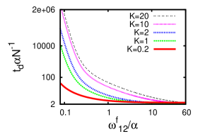
Figure 9: Normalized MFTT $\alpha N^{-1}t_{d}$ plotted against the normalized motor speed $\omega^{f}_{12}/\alpha$ for different values of $K$ with $\omega_{12}/\alpha=\omega_{21}/\alpha=0.5$.

In Fig.9 we plot the normalized MFTT $t_{d}\alpha/N$ as a function of the normalized motor speed $\omega^{f}_{12}/\alpha$ for $\omega_{12}/\alpha=\omega_{21}/\alpha=0.5$ and a few fixed values of the parameter $K$. For any fixed value of $K$, the normalized MFTT decreases monotonically with the increase of the normalized motor speed and saturates to the value given by equation (46) in the limit $\omega^{f}_{12}/\alpha\to\infty$. Moreover, for a given value of $\omega^{f}_{12}/\alpha$, as the flap binding constant $K$ increases the MFTT increases.

(a)

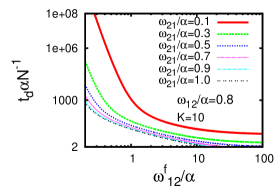
(b)

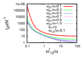
Figure 10: Normalized MFTT $\alpha N^{-1}t_{d}$ plotted against the normalized motor speed $\omega^{f}_{12}/\alpha$ for different values of $\omega_{21}/\alpha$ with (a) $\omega_{12}/\alpha=0.8$, and (b) $\omega_{12}/\alpha=0.1,K=10$.

In Fig.10, $t_{d}$ is plotted against $\omega^{f}_{12}/\alpha$ for (a) $K=10$, $\omega_{12}/\alpha=0.8$, and (b) $K=10$, $\omega_{12}/\alpha=0.1$, each for a few distinct values of $\omega_{21}/\alpha$. The MFTT decreases as $\omega_{21}/\alpha$ increases. This is a consequence of the fact that $\omega_{21}$ depends on the ATP concentration. For small $\omega_{12}/\alpha$ reduces the amplitude of peeling time.

In Fig.11 we demonstrate that for large value of $\omega_{21}/\alpha$, which effectively speeds up the motor, reduces the magnitude of the MFTT.

(a)

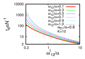
(b)

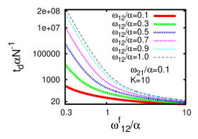
Figure 11: Normalized MFTT $\alpha N^{-1}t_{d}$ plotted against the normalized motor speed $\omega^{f}_{12}/\alpha$ for different values of $\omega_{12}/\alpha$ with (a) $\omega_{21}/\alpha=0.8$, and (b) $\omega_{21}/\alpha=0.1,K=10$.

Although the qualitative trends of variations of $t_{d}$ with $\omega^{f}_{12}/\alpha$ in our model is similar to that in Chou’s model chou , wide range of variation of $t_{d}$ is possible in our model by controlling $\omega_{21}$ which, in turn, can be controlled by the ATP concentration.

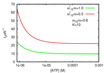
Figure 12: Normalized MFTT $\alpha N^{-1}t_{d}$ plotted against the ATP concentration [ATP] for $\omega_{12}/\alpha=0.1$, $K=10.0$ and two different values of $\omega^{f}_{12}/\alpha$.

In order to explore the dependence of $t_{d}$ on the concentration of ATP, we first assume that

$$\omega_{21}=\omega_{21}^{0}[ATP]$$ (53)

Assuming a typical value $\omega_{21}^{0}=10^{6}M^{-1}s^{-1}$, we have plotted the normalized MFTT against the ATP concentration for two different normalized values of the unhindreed motor speed keeping the other parameters fixed. With the increase of ATP concentration, the MFTT decreases and, gradulally saturates. When ATP concentration is sufficiently high, the step with rate constant $\omega_{21}$ is no longer rate-limiting. We also find that, for a given ATP concentration, the higher is the value of $\omega^{f}_{12}/\alpha$ the shorter is the MFTT $t_{d}$.

The linear dependence of $\omega_{21}$ on ATP concentration, as envisaged in (53), may be valid only at sufficiently low concentration of ATP. In general, $\omega_{21}$ may follow the usual Michaelis-Menten equation for the rate of enzymatic reactions (because $\omega_{21}$ represents the rate of ATP hydrolysis catalyzed by the CRE motor) dixon79 . In that case $\omega_{21}$ itself would saturate with the increase of ATP concentration, instead of increasing linearly with [ATP].

IV Conclusion

In this paper we have studied the process of ATP-dependent chromatin remodeling. For simplicity, we have considered only a single nucleosome consisting of a dsDNA strand wrapped one and three-fourth turns around a cylindrical spool made of histone proteins. We have extended Chou’s model chou by assigning two distinct “chemical” states to the CRE and postulating a minimal mechano-chemical kinetic scheme for capturing the effects of ATP hydrolysis explicitly. Our theoretical framework has been developed exploiting a close analogy with the unzipping of a double-stranded DNA by a helicase garai . We have written down the master equations for the postulated kinetic scheme. This model of footprint traversal by ATP-dependent CRE can be easily interpreted as an implementation of a Brownian ratchet mechanism. From an analytical treatment of this stochastic kinetic model, we have derived analytical expression for the MFTT of the ATP-dependent CRE. We make explicit analytical predictions on the dependence of the MFTT on (i) the unhindred speed of the CRE, as well as on (ii) the concentration of ATP. In principle our theoretical predictions can be tested by carrying out in-vitro experiments with a single nucleosome.

Acknowledgements: DC thanks Michael Poirier and Tom Chou for useful discussion and correspondence, respectively. DC acknowledges support of the Visitors Program of the Max-Planck Institute for the Physics of Complex Systems in Dresden where parts of this work were carried out during two separate visits. DC also thanks Frank Jülicher for discussions in the initial stages of this work and Anirban Sain for a critical reading of the manuscript. This work is also supported, in part, by IIT Kanpur through the Dr. Jag Mohan Chair professorship (DC) and by a research grant from CSIR, India (DC). AG thanks UGC, India, for a senior research fellowship.

References

- (1) A. Wolfee, Chromatin: structure and function, (Academic Press, 1998).
- (2) J. Widom, Annu. Rev. Biophys. Biomol.Struc. 27, 285 (1998).
- (3) H.Schiessel, J. Phys. Condens. Matter, 15, R699 (2003).
- (4) C. Lavelle and A. Benecke, Eur. Phys. J. E 19, 379 (2006).
- (5) R.D. Kornberg and Y. Lorch, Cell 98, 285 (1999).
- (6) K.J. Polach and J. Widom, J. Mol. Biol. 254, 130 (1995).
- (7) J.D. Anderson, A. Thastrom and J. Widom, Mol. Cell. Biol. 22, 7147 (2002).
- (8) H.Y. Fan, X. He, R.E. Kingston and G.J. Narlikar, Mol. Cell 11, 1311 (2003).
- (9) A. Flaus and T. Owen-Hughes, Biopolymers 68, 563 (2003).
- (10) A. Flaus and T. Owen-Hughes, FEBS J. 278, 3579 (2011).
- (11) S.E. Halford, A.J. Welsh and M.D. Szczelkun, Annu. Rev. Biophys. Biomol. Struct. 33, 1 (2004).
- (12) A. Saha, J. Wittmeyer and B.R. Cairns, Nat. Rev. Mol. Cell Biol. 7, 437 (2006).
- (13) C.R. Clapier and B.R. Cairns, Annu. Rev. Biochem. 78, 273 (2009).
- (14) L. R. Racki and G. J. Narlikar, Curr. Opin, Genet. Dev. 18, 137 (2008).
- (15) T. Sakaue, K. Yoshikawa, S.H. Yoshimura and K. Takeyasu, Phys. Rev. Lett. 87, 078105 (2001).
- (16) H. Schiessel, J. Widom, R.F. Bruinsma and W.M. Gelbert, Phys. Rev. Lett. 86, 4414 (2001).
- (17) I.M. Kulic and H. Schiessel, Phys. Rev. Lett. 91, 148103 (2003).
- (18) I.M. Kulic and H. Schiessel, Biophys. J. 84, 3197 (2003).
- (19) H. Schiessel, Eur. Phys. J. E 19, 251 (2006).
- (20) F. Mohammad-Rafiee, I.M. Kulic and H. Schiessel, J. Mol. Biol. 344, 47 (2004).
- (21) R. Blossey and H. Schiwssel, FEBS J. 278, 3619 (2011).
- (22) W. Möbius, R.A. Neher and U. Gerland, Phys. Rev. Lett. 97, 208102 (2006).
- (23) J. Langowski, Eur. Phys. J. E 19, 241 (2006).
- (24) A. Lense and J.M. Victor, Eur. Phys. J. E 19, 279 (2006).
- (25) C. Vaillant, B. Audit, C. Thermes and A. Arneodo, Eur. Phys. J. E 19, 263 (2006).
- (26) P. Ranjith, J. Yan and J.F. Marko, PNAS 104, 13649 (2007).
- (27) G. Lia, E. Praly, H. Ferreira, C. Stockdale, Y.C. Tse-Dinh, D. Dunlap, V. Croquette, D. Bensimon and T. Owen-Hughes, Mol. Cell 21, 417 (2006).
- (28) B.R. Cairns, Nat. Struct. and Mol. Biol. 14, 989 (2007).
- (29) T. Chou, Phys. Rev. Lett., 99, 058105 (2007).
- (30) G. Li, M. Levitus, C. Bustamante and J. Widom, Rapid spontaneous accessibility of nucleosomal DNA, Nat. Struct. Mol. Biol. 12, 46-53 (2004).
- (31) M.G. Poirier, M. Bussiek, J. Langowski, J. Mol. Biol. 379, 772-786 (2008).
- (32) M.G. Poirier, E. Oh, H.S. Tims and J. Widom, Nat. Struct. Mol. Biol. 16, 938 (2009).
- (33) H.S. Tims, K. Gurunathan, M. Levitus and J. Widom, J. Mol. Biol. 411, 430 (2011).
- (34) G. Meersseman, S. Pennings and E.M. Bradbury, EMBO J. 11, 2951 (1992).
- (35) A. Lusser and J.T. kadonaga, BioEssays 25, 1192 (2003).
- (36) P.B. Becker and W. Hörz, Annu Rev. Biochem. 71, 247-273 (2002).
- (37) G. Längst and P.B. Becker, Biochim. Biophys. Acta 1677, 58 (2004).
- (38) A. Garai, D. Chowdhury, M. Betterton, 77, 061910 (2008).
- (39) P.A. Pury and M. O. Caceres, J. Phys. A 36, 2695 (2003).
- (40) M. Dixon and E.C. Webb, Enzymes (Academic Press, 1979).