Bayesian experimental design for the active nitridation of graphite by atomic nitrogen

Abstract

The problem of optimal data collection to efficiently learn the model parameters of a graphite nitridation experiment is studied in the context of Bayesian analysis using both synthetic and real experimental data. The paper emphasizes that the optimal design can be obtained as a result of an information theoretic sensitivity analysis. Thus, the preferred design is where the statistical dependence between the model parameters and observables is the highest possible. In this paper, the statistical dependence between random variables is quantified by mutual information and estimated using a $k$ nearest neighbor based approximation. It is shown, that by monitoring the inference process via measures such as entropy or Kullback-Leibler divergence, one can determine when to stop the data collection process. The methodology is applied to select the most informative designs on both a simulated data set and on an experimental data set, previously published in the literature. It is also shown that the sequential Bayesian analysis used in the experimental design can also be useful in detecting conflicting information between measurements and model predictions.

1 Introduction

The paper examines the problem of optimal data collection in order to calibrate a graphite nitridation model. The calibration of the model is done in the context of Bayesian framework, where the probability distribution of the uncertain parameters is inferred from observations using Bayes’ theorem. Here, the goal of the experimental design is to select the optimal values for the control variables which can be tuned by the experimentalist such that the post-experimental uncertainty in the model parameters is reduced.

Since pre-experimental decisions have to be made before any measurements are taken, it is convenient to frame the design problem also in the Bayesian framework, in order to average over the unknown future observations. A comprehensive and unified view of Bayesian experimental design is given in Chaloner and Verdinelli (1995). In this paper, the optimal design is found to maximize the expected utility when the purpose of the experiment is to estimate the parameters of the mathematical model. Thus the utility function employed in this work is based on Shannon’s measure of information, Shannon (1948), which reflects our goal for parameter estimation as described by Lindley (1956). Other utility functions can be tailored when the purpose of the experiment is prediction, hypothesis testing or mixed objectives including minimizing the financial cost of the experiment.

The proposed approach is applied to a sequential design when the acquisition of the data can be done in the context of experiments on-demand. Such a sequential approach is described by Fedorov (1972) and Loredo and Chernoff (2003) which clearly identify the three stages of the experimental process: experiment - inference - design. The data already collected is used to update the probability density function (pdf) of the parameters, and the result of this inference can be further used in identifying the next design which best resolves our questions of interest in the model. After the experiment is performed, the cycle continues with a new inference step, followed by a design step and so on until the experimental objective is reached.

Due to the high computational complexity of the Bayesian experimental design, its adoption is rather low especially when dealing with nonlinear models. A large body of work can be found in the literature on optimal design for linear or linearized models under the name of Bayesian alphabetic criteria, see DasGupta (1995). However in the recent years a revived interest in Bayes optimal designs for nonlinear models can be attributed to Bayesian recursive update, efficient estimators of information-theoretic measures and to Markov chain Monte Carlo (MCMC) algorithms which can efficiently sample complicated posterior distributions. In Muller (1999), the author makes use of MCMC to create a new simulation-based design, approach which jointly samples from an artificial probability model on the design, data and parameters.

By exploiting the independence property of the noise from the design, Sebastiani and Wynn (1997) extended the maximum entropy sampling proposed by Shewry and Wynn (1987) to estimation problems. They show that the experiment which provides the maximum amount of information for model parameters is the one for which the predictive distribution has the largest entropy. In other words, the most informative experiment is the one where we know the least. A similar information-theoretic approach is presented by Farhang-Mehr and Azarm (2002), which maximizes the entropy of Gaussian priors. These methods are aligned with previous ideas found in Lindley (1956) of incorporating information-theoretic approaches in the experimental design process.

The main contribution of this paper is to emphasize the intuitive interpretation of the Bayesian experimental design as an information-theoretic sensitivity analysis, methodology which is applied to an engineering problem for which real experimental measurements exist. It is shown that the optimal design for estimation problems is the one which maximizes the mutual information of the parameters and the future observations. Given the connection between mutual information and copula functions used to model statistical dependencies, see Calsaverini and Vicente (2009), this new interpretation of Bayesian experimental design reveals that optimal sampling for parameter estimation can be yielded by an information-theoretic sensitivity analysis, see also Appendix B. Thus the optimal design occurs where the statistical dependence between observables and parameters is maximized. In contrast to the maximum entropy sampling, no assumptions are made about the functional dependence of the entropy of conditional distribution on the design.

In the inference stage, we use an adaptive MCMC algorithms proposed by Cheung and Beck (2009) to obtain samples from the posterior distribution of model parameters. Estimators based on $k$-nearest neighbor are used to compute the information theoretic measures required in the design stage. The use of these estimators is advantageous when only samples are available to describe the underlying distributions. The mutual information is estimated using Kraskov’s approach, see Kraskov et al. (2004), which extends the $k$-nearest neighbor based estimator for differential Shannon entropy developed by Kozachenko and Leonenko (1987).

While papers on experimental design can be found in geoscience - Guest and Curtis (2009), neuroscience - Paninski (2005), biomedical applications - Clyde et al. (1996), Chung and Haber (2011), Horesh et al. (2011), engineering - Tucker (2008), just to name a few, the application of Bayesian design principles to actual experiments still lags far behind the theoretical advancements, see Chaloner and Verdinelli (1995). In Curtis and Maurer (2000), the authors compare the small number of papers published on average per year on experimental design to the large number of papers published on inverse methods, emphasizing the disconnect between the amount of data and the amount of information contained in the data. A more efficient learning of model parameters can be accomplished by using Bayesian experimental design which tightly couples the computational modeling, experimental endeavors and data analysis.

In this work, we consider an experiment for the nitridation of graphite conducted by Zhang et al. (2009). The main objective of the experiment is to measure the reaction rate of the graphite with active nitrogen. This quantity is of great importance for assessment of the effectiveness of the thermal protective system of space vehicles. The main parameter of interest is the reaction probability of the graphite nitridation reaction. The values of this quantity presented in the literature (Park and Bogdanoff (2006), Goldstein (1964), Suzuki et al. (2008), Zhang et al. (2009)) vary by several orders of magnitude. The experiments reported in Zhang et al. (2009) have a detailed description of the scenarios with readily available data. The authors conducted a series of runs at different conditions that are not based on experimental design considerations. Hence the effectiveness of a rigorous experimental design strategy can be demonstrated.

In Section 2 the problem of optimal experimental design is described in the Bayesian framework. The experimental setup for the nitridation of graphite is detailed in Section 3, followed by the model description in Section 4. The numerical results for both simulated data and real experimental data are presented in Section 5, and the concluding remarks are given in Section 6.

2 Description of the experimental design

Given a set of observations $D_{n-1}=\{\tilde{\mathbf{d}}_{1},\tilde{\mathbf{d}}_{2},\ldots,\tilde{\mathbf{d}}_{n-1}\}$ we are concerned with finding the next experimental design $\boldsymbol{\xi}_{n}\in\boldsymbol{\Xi}$ such that the model parametric uncertainty is reduced after the experiment is performed and the associated measurement data $\tilde{\mathbf{d}}_{n}$ is collected. The mathematical models used in this paper are generally represented by the following abstract model:

$$\mathbf{r}(\mathbf{u},\boldsymbol{\theta},\boldsymbol{\xi},\boldsymbol{\epsilon}_{s}) = \mathbf{0}$$ (1)

$$\mathbf{d} = \mathbf{d}(\mathbf{u},\boldsymbol{\theta},\boldsymbol{\xi},\boldsymbol{\epsilon}_{m})$$ (2)

Here $\mathbf{u}$ is the state of the system which obeys the governing equations defined by $\mathbf{r}(\cdot)$, $\boldsymbol{\xi}\in\boldsymbol{\Xi}$ is the control variables associated with the experimental scenario, $\boldsymbol{\Xi}$ is the design space and $\boldsymbol{\theta}\in\Theta$ are the model parameters, where $\Theta$ is the parameter space of the model. Here, the model prediction $\mathbf{d}_{n}$ calculated using the measurement model $\mathbf{d}(\cdot)$ is comparable with the experimental data $\tilde{\mathbf{d}}_{n}$ for a particular scenario input $\boldsymbol{\xi}_{n}$. The random vector or random field $\boldsymbol{\epsilon}_{s}$ captures any stochastic forcing present in the governing equations such as unmodeled dynamics and $\boldsymbol{\epsilon}_{m}$ models the discrepancy between model predictions and experimental data.

2.1 Bayesian experimental design

In the followings it is assumed that we can afford to perform up to $N$ experiments to obtain the desired measurements. Preferably, one will want to perform as few informative experiments as possible in order to calibrate the model. The experimental design process employed in this paper generates an optimal sequence of designs such that the information gain is maximized after each experiment. More about this sequential process of designing experiments can be found in Fedorov (1972). Note that since this decision process is sequential, and the next design depends on the previous experiments, it does not guarantee to find the optimal $N$ designs among all possible combinations of $N$ designs. This would correspond to a batch update of the prior parametric uncertainty and an expensive combinatorial decision process, which would require a large number of Monte Carlo samples to estimate the necessary expected utilities for each possible combination of designs.

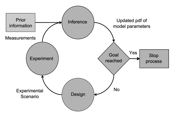
Figure 1: Schematic of sequential experimental design process

The entire experimental process is divided in three stages: experiment stage, inference stage and, design stage. In the experiment stage, new data is collected according to the strategy obtained in the previous design stage. Initially, this data can also be obtained from any experiments documented in the literature that are related with the underlying modeling problem. In the inference stage, the newly obtained experimental data is used to update the prior pdf of the model parameters using Bayes rule. The resulting pdf is further used to predict the distribution of the future observations for a variety of scenarios which cover the design space. The best design is chosen by maximizing the expected Shannon information gain, expectation taking with respect to the distribution of future data. The experimental process is depicted in Fig.1.

2.2 Bayesian inference step

The inference stage consists in applying Bayes’s theorem to calculate the distribution of the model parameters conditioned on all the available data, $p(\boldsymbol{\theta}|D_{n})$. Using the conditioning rule, one can derive the following recursive Bayesian update:

$$p(\boldsymbol{\theta}|D_{n}) = \frac{p(D_{n}|\boldsymbol{\theta})p(\boldsymbol{\theta})}{p(D_{n})}$$ (3)

$$= \frac{p(\tilde{\mathbf{d}}_{n},D_{n-1}|\boldsymbol{\theta})p(\boldsymbol{\theta})}{p(\tilde{\mathbf{d}}_{n},D_{n-1})}$$

$$= \frac{p(\tilde{\mathbf{d}}_{n}|D_{n-1},\boldsymbol{\theta})p(D_{n-1}|\boldsymbol{\theta})p(\boldsymbol{\theta})}{p(\tilde{\mathbf{d}}_{n}|D_{n-1})p(D_{n-1})}$$

$$= \frac{p(\tilde{\mathbf{d}}_{n}|D_{n-1},\boldsymbol{\theta},\boldsymbol{\xi}_{n})p(\boldsymbol{\theta}|D_{n-1})}{p(\tilde{\mathbf{d}}_{n}|D_{n-1},\boldsymbol{\xi}_{n})}$$

Under the assumption of conditionally independent measurements given model parameters, then the above expression can be simplified using the following relation: $p(\tilde{\mathbf{d}}_{n}|D_{n-1},\boldsymbol{\theta},\boldsymbol{\xi}_{n})=p(\tilde{\mathbf{d}}_{n}|\boldsymbol{\theta},\boldsymbol{\xi}_{n})$. The denominator is given by,

$$p(\tilde{\mathbf{d}}_{n}|D_{n-1},\boldsymbol{\xi}_{n})=\int_{\Theta}p(\tilde{\mathbf{d}}_{n}|\boldsymbol{\theta},\boldsymbol{\xi}_{n})p(\boldsymbol{\theta}|D_{n-1})\mathrm{d}\boldsymbol{\theta}$$ (4)

and quantifies the evidence provided by the new experimental data, $\tilde{\mathbf{d}}_{n}$, in support of our model conditioned on all the previous measured data. The use of Bayesian inference in the sequential experimental design is advantageous as it permits the iterative accumulation of information. The posterior distribution obtained in this stage becomes the prior distribution in the next stage of inference. After all the $N$ experiments have been performed, the last posterior distribution summarizes the information contained in all the available measurements.

Instead of performing $N$ experiments, the data collection process can be stopped earlier, when precision measures computed in the interim stages, such as the determinant of the sample covariance matrix, satisfy the thresholds predefined by the user. The process can also be ceased when the rate of reducing the uncertainty in the parameters has slowed enough or when indication exists that model predictions and the corresponding experimental observations are in disagreement.

The inverse problem of calibrating the model parameters from the measurement data is solved using Markov chain Monte Carlo simulations. In our simulations, samples from the posterior distribution $\boldsymbol{\theta}\sim p(\boldsymbol{\theta}|D_{n})$ are obtained using the statistical library QUESO Prudencio and Schulz (2011) equipped with the Hybrid Gibbs Transitional Markov Chain Monte Carlo method proposed by Cheung and Beck (2008, 2009).

2.3 Optimal experimental design step

According to Lindley (1956) when the objective of the experiment is to learn about the model parameters $\boldsymbol{\theta}$, then the utility function is given by the amount of information provided by the measurement $\tilde{\mathbf{d}}_{n}$ as result of performing the experiment with the design $\boldsymbol{\xi}_{n}$. Since $\tilde{\mathbf{d}}_{n}$ has not yet been observed, and we have to make a decision regarding the design $\boldsymbol{\xi}_{n}$ prior to the experiment, in the following, we are using the unknown measurement $\mathbf{d}_{n}$ and its corresponding predictive distribution.

$$U(\mathbf{d}_{n},\boldsymbol{\xi}_{n}) = \int_{\boldsymbol{\Theta}}p(\boldsymbol{\theta}|\mathbf{d}_{n},D_{n-1})\log p(\boldsymbol{\theta}|\mathbf{d}_{n},D_{n-1})\mathrm{d}\boldsymbol{\theta}$$ (5)

$$-\int_{\boldsymbol{\Theta}}p(\boldsymbol{\theta}|D_{n-1})\log p(\boldsymbol{\theta}|D_{n-1})\mathrm{d}\boldsymbol{\theta}$$

Here, the prior pdf for model parameters is given by $p(\boldsymbol{\theta}|D_{n-1})$, and it is used to compute the following predictive distribution for the observables when the input scenario is $\boldsymbol{\xi}_{n}$:

$$p(\mathbf{d}_{n}|D_{n-1},\boldsymbol{\xi}_{n})=\int_{\Theta}p(\mathbf{d}_{n}|\boldsymbol{\theta},\boldsymbol{\xi}_{n})p(\boldsymbol{\theta}|D_{n-1})\mathrm{d}\boldsymbol{\theta}$$ (6)

Since we are in the pre-experimental stage, we can compute the average amount of information provided by an experiment $\boldsymbol{\xi}_{n}$ by marginalizing over all the unknown future observations:

$$\mathrm{E}_{\mathbf{d}_{n}}[U(\mathbf{d}_{n},\boldsymbol{\xi}_{n})]=\int_{\mathcal{D}}U(\mathbf{d}_{n},\boldsymbol{\xi}_{n})p(\mathbf{d}_{n}|D_{n-1},\boldsymbol{\xi}_{n})\mathrm{d}\mathbf{d}_{n}$$ (7)

The optimal experiment is obtained by solving the following optimization problem:

$$\boldsymbol{\xi}_{n}^{*}=\arg\max_{\boldsymbol{\xi}_{n}\in\boldsymbol{\Xi}}\mathrm{E}_{\mathbf{d}_{n}}[U(\mathbf{d}_{n},\boldsymbol{\xi}_{n})]$$ (8)

By substituting Eq.(5) into Eq.(7), the expected utility can be written in the following form:

$$\mathrm{E}_{\mathbf{d}_{n}}[U(\mathbf{d}_{n},\boldsymbol{\xi}_{n})] = \int_{\mathcal{D}}\int_{\boldsymbol{\Theta}}p(\boldsymbol{\theta},\mathbf{d}_{n}|D_{n-1},\boldsymbol{\xi}_{n})\log\frac{p(\boldsymbol{\theta},\mathbf{d}_{n}|D_{n-1},\boldsymbol{\xi}_{n})}{p(\mathbf{d}_{n}|D_{n-1},\boldsymbol{\xi}_{n})}\mathrm{d}\boldsymbol{\theta}\mathrm{d}\mathbf{d}_{n}$$

$$-\int_{\mathcal{D}}\int_{\boldsymbol{\Theta}}p(\boldsymbol{\theta},\mathbf{d}_{n}|D_{n-1},\boldsymbol{\xi}_{n})\log p(\boldsymbol{\theta}|D_{n-1})\mathrm{d}\boldsymbol{\theta}\mathrm{d}\mathbf{d}_{n}$$

$$= \int_{\mathcal{D}}\int_{\boldsymbol{\Theta}}p(\boldsymbol{\theta},\mathbf{d}_{n}|D_{n-1},\boldsymbol{\xi}_{n})\log\frac{p(\boldsymbol{\theta},\mathbf{d}_{n}|D_{n-1},\boldsymbol{\xi}_{n})}{p(\boldsymbol{\theta}|D_{n-1})p(\mathbf{d}_{n}|D_{n-1},\boldsymbol{\xi}_{n})}\mathrm{d}\boldsymbol{\theta}\mathrm{d}\mathbf{d}_{n}$$

$$= \mathrm{I}(\boldsymbol{\theta};\mathbf{d}_{n}|D_{n-1},\boldsymbol{\xi}_{n})$$ (10)

Therefore the optimal experiment is the one which maximizes the mutual information between the model parameters and the model predictions. In other words we would like to sample where the expected observations have the highest impact on model parameters.

$$\boldsymbol{\xi}_{n}^{*}=\arg\max_{\boldsymbol{\xi}_{n}\in\boldsymbol{\Xi}}\mathrm{I}(\boldsymbol{\theta};\mathbf{d}_{n}|D_{n-1},\boldsymbol{\xi}_{n})$$ (11)

From information theory, see, for example Cover and Thomas (1991), mutual information quantifies the reduction in uncertainty that knowing the model parameters provides about the model predictions and vice-versa. Being written as the Kullback-Leibler divergence between the joint distribution of parameters and predictions, and the product of their marginals, we can also say that mutual information provides a measure of statistical dependence between the two random variables. This has been shown more formally in Calsaverini and Vicente (2009) by making the connection between mutual information and copula functions which are used to model the dependence between random variables. For completeness this connection is also presented in Appendix B. It turns out that the mutual information is just the negative copula entropy. Hence, mutual information is independent on the marginal distributions and it quantifies only the dependence information contained in the copula function.

In neuroscience, Paninski (2005) uses the same Bayesian optimal design based on maximizing the mutual information between model parameters and model predictions. It is shown that the information-maximization sampling is asymptotically more efficient than an independent and identically distributed sampling strategy. Compared with maximum entropy sampling for parameter estimation proposed by Sebastini and Wynn (2000), the sampling based on maximizing the mutual information is more general, no assumption about the independence assumption is made about the discrepancy model with respect to the design.

Finally, in the design step, the experimental space $\boldsymbol{\Xi}$ is discretized and the corresponding marginal distributions of model predictions and parameters, as well as the joint pdf of the two are computed. The mutual information corresponding to each experimental design is calculated as in Subsection 2.4, and the design corresponding to the highest MI is selected for the next experiment. Here, samples from the joint distribution of parameters and model predictions are obtained using Monte Carlo simulations according to the following relation:

$$p(\mathbf{d}_{n},\boldsymbol{\theta}|D_{n-1},\boldsymbol{\xi}_{n})=p(\mathbf{d}_{n}|\boldsymbol{\theta},\boldsymbol{\xi}_{n})p(\boldsymbol{\theta}|D_{n-1})$$ (12)

2.4 Estimating the mutual information

The estimation of the mutual information in this paper is done using the $k$NN (Nearest Neighbor) method proposed by Kraskov et al. (2004). This is based on the $k$NN estimator for the entropy proposed by Kozachenko and Leonenko (1987). The entropy of a random variable can be approximated from $N$ samples using Kozachenko-Leonenko’s estimator:

$$\mathrm{H}(X)\approx-\psi(k)+\psi(N)+\frac{d_{X}}{N}\sum_{i=1}^{N}\log\epsilon(i)$$ (13)

where $\psi(\cdot)$ is the digamma function, $d_{X}$ is the dimensionality of the random variable $X$, and $\epsilon(i)$ is the distance from sample $X_{i}$ to its $k$NN, $X_{k(i)}$, and is given by the maximum norm:

$$\epsilon(i)=\|X_{i}-X_{k(i)}\|_{\infty}$$ (14)

This is a biased estimator due to the assumption of local uniformity of the density. By definition, the MI can be decomposed as the sum of marginal entropies minus the joint entropy. Therefore, the above estimator can be used to approximate all three entropies and thus the mutual information. However the errors made in estimating individual entropies will not cancel out in general. To partially alleviate this problem, Kraskov’s approach is not to fix $k$ when estimating the marginal entropies. It can be shown, see Kraskov et al. (2004), that the MI of the parameters and model prediction can be computed as follows:

$$\mathrm{I}(\boldsymbol{\theta};\mathbf{d}_{n}|D_{n-1},\boldsymbol{\xi}_{n})\approx\psi(k)-\frac{1}{N}\sum_{i=1}^{N}\bigg{(}\psi(n_{\theta}(i)+1)+\psi(n_{d}(i)+1)\bigg{)}+\psi(N)$$ (15)

where $n_{d}(i)$ and $n_{\theta}(i)$ are the number of points in the marginal space within $\epsilon(i)$ distance from the $i$th sample. Here, $\epsilon(i)$ is the distance from the $i$th sample to its $k$NN in the joint space.

Based on numerical studies, Khan et al. (2007) shows that the estimators based on $k$NN and kernel density estimation (KDE) outperform commonly used dependence measures such as linear correlation, cross-correlogram or Kendall’s $\tau$. Furthermore, it is also shown that in general the $k$NN estimator captures better the nonlinear dependence than the KDE. However the Kraskov’s MI estimator has to be used with care. A small value for $k$ will result in a small bias but a larger variance and vice-versa. Also, the efficiency of the estimator decreases as the dimensionality of the joint space increases.

For completeness, an example test has been carried out to show the performance of the $k$NN estimator for the MI as function of the dimensionality for the joint space, the number of the samples and the number of $k$NN’s. The joint pdf of two random variables of known dimensions is modeled using a Gaussian density function for which we can compute the exact MI. For each combination of joint dimensionality, $k$NN, and sample size, a number of $1000$ trial runs have been used to generate samples according to the Gaussian density function. The entries in the covariance matrix have been considered to be $1$ on the diagonal and $0.9$ for the off-diagonal elements. Using the true value of the MI and the estimated value, one can compute the relative absolute error for each run. The result of the average absolute relative error over the $1000$ trial runs is shown in Table 1.

2.5 Example $1$: Simulation experiment

Consider the following nonlinear design problem:

$$d=\theta_{1}\xi+\theta_{2}\xi^{2}+f(\xi)\epsilon$$ (16)

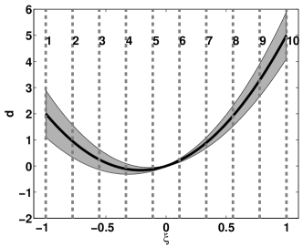
(a) Initial response (additive noise)

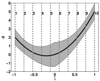
(b) Initial response (multiplicative noise)

Figure 2: Results for example $1$. Model response given initial discrepancy and parametric uncertainty.

The goal of the experiment design in this example is to efficiently learn the model parameters, $\theta_{1}$ and $\theta_{2}$, when the design space is given by $\Xi=[-1,1]$. The discrepancy model is given by $f(\xi)\epsilon$, where $\epsilon$ is a standard normal random variable, $\mathcal{N}(0,1)$. The two parameters are uniformly distributed according to $\theta_{1}\sim\mathcal{U}(1,2)$ and $\theta_{2}\sim\mathcal{U}(3,4)$. Two cases are analyzed: additive noise when $f(\xi)=0.01$ and multiplicative noise with respect to the design when $f(\xi)=0.5(1.1-|\xi|)$. Given the initial uncertainty of the parameters and the discrepancy function, the response of the model it is shown in Figs.2(a)-2(b). In this respect we want to compare the maximum entropy sampling with the information maximization sampling described in this paper. Hence, the two cost functions to be maximized in the design stage are,

• $J(\xi_{n})=\mathrm{I}((\theta_{1},\theta_{2});d_{n}|D_{n-1},\xi_{n})$ for information maximization (IM) sampling

• $J(\xi_{n})=\mathrm{H}(d_{n}|D_{n-1},\xi_{n})$ for maximum entropy (ME) sampling

The two sampling approaches, IM and ME, are also compared with a strategy based on random sampling (RND), which at each stage it randomly chooses a design. All the designs being equally likely at every stage.

In this example we consider that up to $10$ experiments can be performed with scenario values equally distributed in the design space as indicated by the dashed lines in Figs.2(a)-2(b). For each case corresponding to the discrepancy function, additive noise or multiplicative noise, two other cases are analyzed with respect to experimental sampling restriction. In the first case no repeated measurements are allowed. Thus, once an experimental design has been chosen from the set of $10$ designs, it can no longer be used in the subsequent stages. The second case corresponds to allowing repeated measurements in our calibration. Synthetic measurements are created using Eq.(16), where the true value of the parameters are set to $\theta_{1}=1.5$ and $\theta_{2}=3.5$. A different noise sample has been generated for each of the $10$ scenarios. For this example we have used $2000$ samples in computing the MI and the $kNN$ has been set to $6$.

For the two cases considered in this example (additive and multiplicative noise) each strategy will yield a sequence of designs. At each stage of the design, the performance of each strategy is given by the reduction in uncertainty of the parameters which is quantified by the entropy of the parameter distribution. The entropy is computed here using Eq.(13) and for comparison purposes, since we are generating synthetic measurements and use a random sampling approach, the entropy is averaged over $100$ Monte Carlo runs.

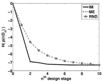
(a) Average entropy (additive noise - repeated measurements not allowed)

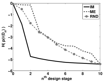
(b) Average entropy (multiplicative noise - repeated measurements not allowed)

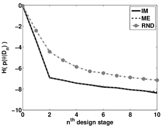
(c) Average entropy (additive noise - repeated measurements allowed)

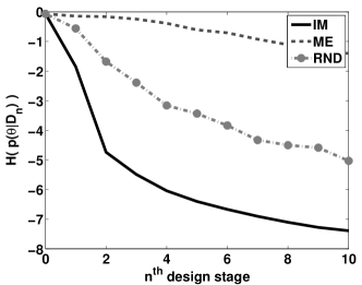
(d) Average entropy (multiplicative noise - repeated measurements allowed)

Figure 3: The evolution of the entropy of parameter distribution averaged over $100$ Monte Carlo runs for the three strategies: IM - Information Maximization Sampling, ME - Maximum Entropy Sampling, RND - Random Sampling, and the two case: no repeated measurements and repeated measurements.

As expected, for the additive noise the maximum entropy sampling is equivalent to the information maximization sampling as it is shown in Fig.3(a) and Fig.3(c). Table 2 shows that in this case the highest initial reduction in uncertainty is obtained by starting the sampling at the boundary of the design domain. For multiplicative noise however, due to the discrepancy model used, the maximum entropy is forced to start the sampling using the design points in the middle of the domain, where the uncertainty is the highest, see Table 3 and Fig.2(b). Because of the distribution of the noise, the performance of the maximum entropy strategy is worse on average even compared with the random sampling.

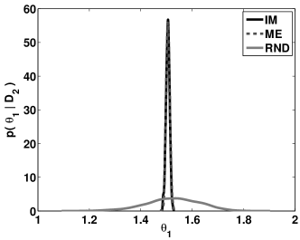
(a) $p(\theta_{1},D_{2})$ (additive noise)

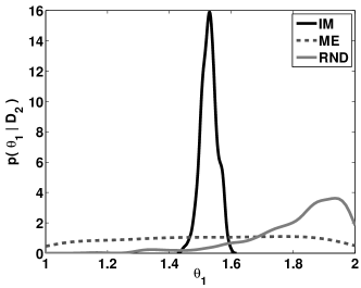
(b) $p(\theta_{1},D_{2})$ (multiplicative noise)

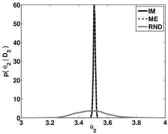
(c) $p(\theta_{2},D_{2})$ (additive noise)

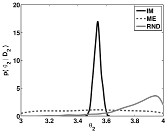
(d) $p(\theta_{2},D_{2})$ (multiplicative noise)

Figure 4: Results for example $1$. Marginal pdfs of model parameters given by the three strategies after the second experimental design stage

A faster reduction in uncertainty is obtained in this case using the information maximization sampling as it is shown in Fig.3(b) and Fig.3(d). For both additive and multiplicative noise cases, an accurate approximation to the true value of the parameters is given by the information maximization sampling using only two experiments as it is shown in Figs.4(a)-4(d). Therefore, an efficient learning of model parameters in the general nonlinear design problems can be achieved using information maximization sampling.

Regarding the experimental sampling restriction, in both cases when we allow and do not allow repetitive measurements the performance of IM is superior when compared with ME and RND, see Fig.3. When repeated measurements are allowed and we have additive noise, both IM and ME consistently select the same boundary design points, see Table 2. For multiplicative noise and repeated measurements, we have the same consistency in choosing the designs, IM selecting the boundary design points while ME selecting the middle design points, which in this case are the least informative designs. This explains the poor performance of ME compared with IM and RND, see Fig.3(d).

3 A description of experimental setup and data

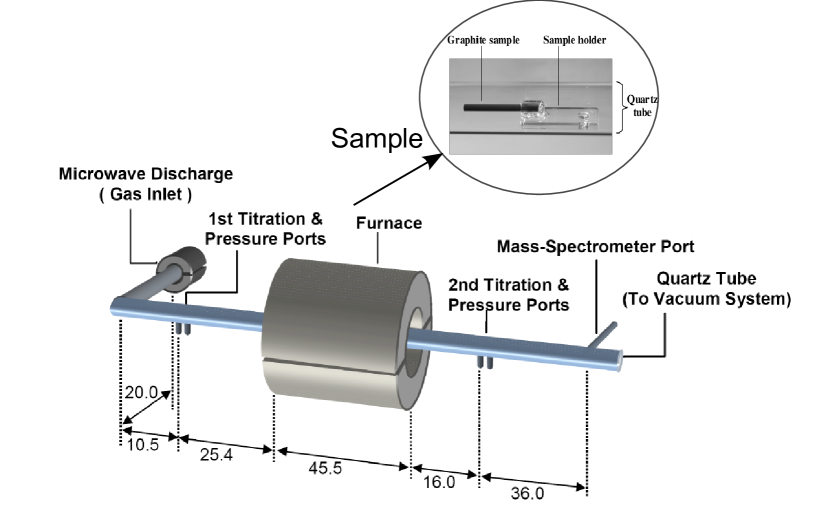
Figure 10: Schematic of the experimental setup used in Zhang et al. (2009). Also shown in the inset is the sample and sample holder

The experimental scenario is described in much detail in Zhang et al. (2009). For completeness, we briefly describe the experimental set-up, the measurements and their associated uncertainties. The experiments were performed to measure the reaction probability of the graphite nitridation reaction, $C_{\text{Gr}}+\text{N}\rightarrow\text{CN}$. The high-purity graphite (grade DFP-2) in the form of 3.175 mm diameter rods was used as the sample. The sample was placed in a furnace-heated quartz tube shown in Fig. 10. A quartz flow tube (22 mm inner diameter) extended through a high-temperature tube furnace with a hot region of approximately 45.5 cm. Atomic nitrogen was generated by flowing nitrogen through a microwave discharge located upstream of the furnace. The microwave discharge was operated at a constant power of around 90-95 W under steady-state temperature and gas flow conditions. The pressure was measured before and after the furnace using a 10 torr Baratron capacitance manometer. The data sheet from the instrument reports uncertainty as $\pm 1\%$ of the recorded value. The temperatures of the flow tube were measured using Omega stick-on type K thermocouples at the location of both pressure ports and near the entrance and exit of the furnace. Temperatures were monitored periodically to ensure steady state operation. The gas pressure and bulk velocity in the flow tube were varied by simultaneous adjustment of the incoming N₂ flow rate with a throttling valve located in the downstream pumping manifold. The uncertainty in the flow rate is quoted as being no more than $1\%$. The mole fraction of atomic nitrogen entering and exiting the furnace were measured by gas phase titration with nitric oxide. In this method, controlled quantities of nitric oxide (NO) is introduced into the titration region. The NO reacts extremely rapidly with atomic N and the disappearance of the NO signals the titration end point.

The nitrogen atoms that strike the graphite surface react with the graphite sample and cause mass loss. Each sample was weighed immediately before it was placed into the flow tube and immediately after it was removed from the flow tube, using a Mettler Toledo XP105 analytic balance with a 0.01 mg resolution. Control experiments were run at various conditions without the microwave discharge to measure the extra mass loss that occurs due to de-volatilization of some residual hydrocarbons in the sample or reaction with oxygen leaking into the flow system. The measured mass loss was adjusted by subtracting the control mass loss. The mass loss rate was obtained by dividing by the time span of the experiment. The most extensive set of measurements have been performed at furnace temperature of 1273 K. The measurements that are required for the calibration of various parameters described in Section 4 are pressure exiting the furnace, and the mass loss of the sample.

4 Model description and uncertain parameters

In this section, we present the model that is used to compute the measured data as a function of model and control parameters, the system defined abstractly in Eq. (1) in Section 2. The experiment (Zhang et al. (2009)) is briefly described in Section 3. Since the focus of this work is not in the detailed physical modeling but in the investigation of most informed experimental design strategy, we use an extremely simplified model with several assumptions proposed by Zhang et al. (2009). The flow is assumed to be one dimensional and given by the Hagen-Poisseuille flow model with temperature varying density given by the ideal gas law. The bulk flow consists entirely of nitrogen as the concentrations of atomic nitrogen and cyanates are negligibly small.

Temperature is assumed to not vary with tube radius. The temperature along the cross section of a tube is the same as the wall temperature. The wall temperature is linearly interpolated between known temperature values along the tube length. The extra pressure drop due to the sample holder is taken into account by using an effective tube diameter in the Hagen-Poisseuille flow model. With these assumptions the pressure, mean velocity and density profiles along the tube are obtained by solving:

$$P\frac{dP}{dz} = -\frac{128\dot{m}_{N_{2}}\mu_{N_{2}}RT(z)}{\pi d_{eff}^{4}W_{N_{2}}}$$ (17)

$$v(z) = \frac{4.0\dot{m}_{N_{2}}}{\rho(z)\pi d_{eff}^{2}}$$ (18)

$$\rho(z) = \frac{P(z)W_{N_{2}}}{RT}$$ (19)

$$P(z=0) = P_{1};\quad v(z=0)=U_{1};\quad T(z)=\Psi(z)$$ (20)

In the above $P(z)$ denotes the temperature as a function of length along the tube $z$, $v(z)$ is the bulk flow velocity, $\dot{m}_{N_{2}}$ is the mass flow rate of N₂, $\rho(z)$ is the density of N₂, $T(z)$ is the temperature of the wall and also the fluid along the tube given by interpolating measured temperatures ($\Psi(z)$ is the linear interpolant), $d_{eff}$ is the effective diameter, $W_{N_{2}}$ is the molecular weight of N₂, $P_{in}$ and $U_{in}$ are the inlet pressure and velocity respectively and $R$ is the universal gas constant. In Eq. (17), Sutherland’s model is used for the viscosity. Thus, $\mu_{N_{2}}=\mu_{ref,N_{2}}\left(\frac{T_{ref}+S_{N_{2}}}{T+S_{N_{2}}}\right)\left(\frac{T}{T_{ref}}\right)^{3/2}$. The constants appearing in Sutherland’s model are also assumed to be known precisely. They are: $\mu_{ref,N_{2}}=0.01781e-3$ Pa s, $S_{N_{2}}=111.0$ and $T_{ref}=300.55$ K.

We also need the values of the nitrogen atom concentration as a function of z. The nitrogen atom concentration is also assumed to not vary with the tube radius. This means that diffusive processes for the N-atom as well as the temperature are assumed to be instantaneous. The assumption is justified due to the small radius, reasonably high speed flow and relatively slow wall recombination reactions. With these assumptions, the $N$-atom concentration profile along the tube is obtained by solving:

$$\frac{d(v(z)C_{N})}{dz} = -\frac{\gamma_{N}(T)\bar{v}_{N}(T)C_{N}}{d_{eff}}-2k(T)C_{N_{2}}C_{N}^{2}$$ (21)

$$C_{N}(z=0) = C_{N,1}$$ (22)

$C_{N}$ is the molar concentration of atomic N, $\gamma_{N}$ is the reaction coefficient for reactions with the quartz wall defined below in Eq. (24), $k(T)$ is the reaction rate for gas phase recombination of N atoms defined in Eq. (23), $\bar{v}_{N}(T)$ is the thermal velocity of N atoms given by kinetic theory defined below in Eq. (25), $C_{N_{2}}$ is the concentration of N₂ gas. The first term in the right hand side models the loss of $N$ atoms as a result of recombination at the wall, the second term accounts for the loss of $N$ atoms due to reaction in the gas phase to produce molecular nitrogen $N_{2}$. The models/definitions for the varies quantities introduced are:

$$k(T) = A_{NN}exp\left[-\frac{E_{a,NN}}{RT}\right]$$ (23)

$$\gamma_{N}(T) = \gamma_{N}(T_{ref})\left(\frac{T}{T_{ref}}\right)^{\alpha}$$ (24)

$$\bar{v}_{N}(T) = \sqrt{\frac{RT}{2\pi W_{N}}}$$ (25)

We assume that sublimation is negligible. The only reaction is a global first order reaction between the solid graphite and nitrogen atom to give CN gas: $C(Gr)+N\rightarrow CN$. In the chosen model, called the Gas Kinetic (GK-) model, the transport of the nitrogen atoms to the surface is assumed to be instantaneous. The backward reaction is ignored. Hence for the GK - model, the mass loss of carbon is given by the following:

$$\Delta M_{C}=\left(\Delta t\pi d_{sample}W_{C}\right)\left(\int_{z=z_{s}}^{z_{s}+L_{s}}C_{N}(z)\sqrt{T(z)}\beta_{N}dz\right)\sqrt{\frac{R}{2\pi W_{N}}}$$ (26)

The main quantity of interest for this experiment is the nitridation coefficient $\beta_{N}$. $\Delta t$ is the time interval of the test, $d_{sample}$ is the diameter of the sample, $W_{C}$ is the molecular weight of carbon, $z_{s}$ is the sample location, $L_{s}$ is the length of the sample and $C_{N}(z)$ is the molar concentration of N along the sample obtained by solution of Eq. (21). In Eq. (26), only the forward equation is considered and the wall concentration of $N$ is the same as the free stream concentration.

In the following, the mass loss and the output pressure $\mathbf{d}_{n}=\{\Delta m_{C},P_{2}\}$, are used as the observables. They can be obtained as a solution of equations (17) and (26) along with the supplementary equations (18) to (25). From a review of the literature, we choose the most uncertain parameters to be $\boldsymbol{\theta}=\{d_{eff},\gamma_{N},\beta_{N}\}$. The stochastic forcing term $\boldsymbol{\epsilon}_{s}$ in Eq. (1) is neglected. The discrepancy term $\boldsymbol{\epsilon}_{m}$ in Eq. (2) is a Gaussian random variable whose 95$\%$ confidence interval is taken to be the estimated error quoted in Zhang et al. (2009), and it is used here to define the likelihood function in the Bayesian inversion. The control variables are the volumetric flow rate, inlet pressure and the inlet N atom mole fraction : $\boldsymbol{\xi}_{n}=\{$ $F_{N_{2},in}$, $P_{1}$, $\mathcal{X}_{N,1}$ $\}$ from which the mass flow rate, $\dot{m}_{N_{2}}$ and inlet nitrogen atom concentration $C_{N,1}$ defined in Eqs. (18) and (22) can be computed.

5 Results

To recapitulate, the most uncertain parameters appearing in the model formulation described in Section 4 are the effective diameter $d_{eff}$, the reaction efficiency $\gamma_{N}$ and, the nitridation coefficient $\beta_{N}$. To learn the model parameters $\boldsymbol{\theta}=\{d_{eff},\gamma_{N},\beta_{N}\}$ the mass loss and the output pressure are used as observables, $\mathbf{d}_{n}=\{\Delta m_{C},P_{2}\}$. In the followings we present the experimental design analysis on both simulated data and real experimental data as given in Zhang et al. (2009). For these examples, we have used $1000$ samples per level in our adaptive MCMC and $2000$ samples at the last level. These $2000$ samples have also been used in the forward uncertainty propagation and in the MI calculation. We have set the $k$NN to $6$ in the following results.

5.1 Example $2$: Simulated measurements

In this example we use the model presented in Section 4 to generate synthetic measurements for pressure and mass loss by adding noise to model predictions using $1\%$ uncertainty for pressure and $5\%$ uncertainty for mass loss. To generate the measurements the following values have been used for the normalized parameters: $\frac{d_{eff}}{d_{eff0}}=0.95$, $\log\bigg{(}\frac{\gamma_{N}}{\gamma_{N0}}\bigg{)}=1.0$ and, $\frac{\beta_{N}}{\beta_{N0}}=2.0$, where the nominal values are given by: $d_{eff0}=0.022$, $\gamma_{N0}=10^{-3}$, and $\beta_{N0}=3.29\times 10^{-}3$.

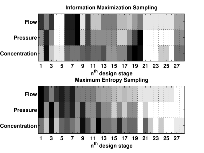
Figure 7: Results for example $2$ (simulated data). Graphical representation for the inflow conditions selected by the two information theoretic strategies. Darker shadings indicate large inflow conditions such as flow, pressure, and concentration.

The values for the experimental scenarios ($F_{N_{2},in}$, $P_{1}$, $\mathcal{X}_{N,1}$, $\Delta t$, $L_{S}$) are the same as in Zhang et al. (2009), and presented in Fig.7. Similar with the previous example three strategies are used to select the optimal sequence of designs from the set of $28$ designs: maximum entropy sampling, information maximization sampling and, ascending sampling which starts with the first tabulated design in Zhang et al. (2009) (enumerated in Fig.7 from $E0$ to $E27$), and continues providing the next available one at each stage.

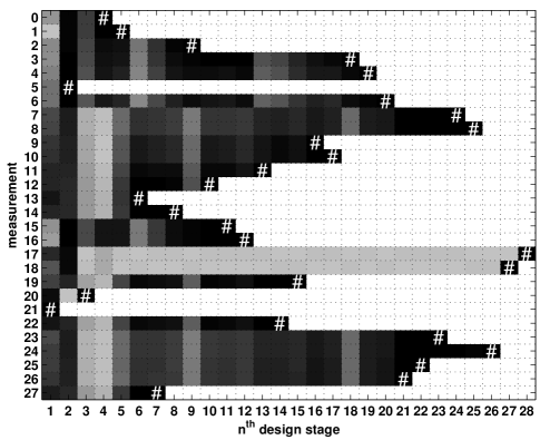
(a) IM: Relative mutual information

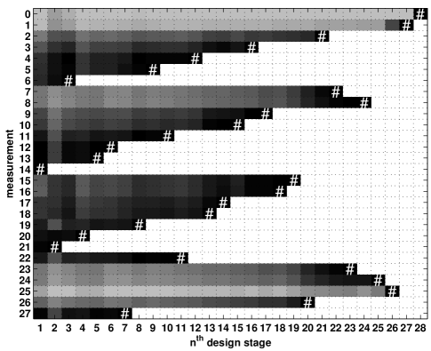
(b) ME: Relative entropy

Figure 6: Results for example $2$ (simulated data). Relative expected utility for Information Maximization Sampling and Maximum Entropy Sampling. Darker shadings indicate large expected utilities (mutual information for IM or entropy for ME) relative to all available scenarios within a design stage. The $\#$ sign indicates which scenario has been selected at a given stage. Previously selected scenarios are excluded from subsequent analysis which is indicated here by white cells.

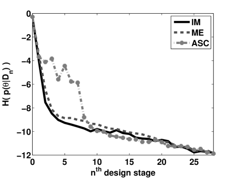
(a) Entropy

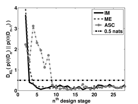
(b) Kullback Leibler divergence

Figure 8: Results for example $2$ (simulated data). The evolution of the entropy and the KL divergence given the posterior distributions yielded by the three strategies for experimental design: IM - Information Maximization Sampling, ME - Maximum Entropy Sampling and ASC - Ascending Sampling

Fig.8(a) shows the drop in uncertainty versus the number of design stages. The design sequences provided by both maximum entropy sampling and the information maximization sampling, see Table 4, give a comparable learning rate, which is superior to the ascending sampling. Fig. 6 gives the relative entropy for ME sampling and relative mutual information for IM sampling at each design stage. The difference between the information theoretic approaches and the ascending sampling is that the former ones give higher priority to the designs with high inflow.

ME sampling preferably selects the experimental scenarios with large values for inflow conditions, either $F_{N_{2},in}$, $P_{1}$, $\mathcal{X}_{N,1}$. For example, first the scenario of 14^th measurement has the largest inflow rate and pressure among others. It follows the same type of experimental scenario. A physical explanation for this trend could be hypothesized as follows. A large value of $F_{N_{2},in}$ results in the large pressure drop through the experimental region. This enhances the sensitivity of pressure on $d_{eff}$ through Eq.(18). Also, a large pressure (e.g., 14^th, 6^th measurements) accelerates chemical reactions especially the gas-phase recombination through the three-body reaction: $N+N+N_{2}\leftrightarrow N_{2}+N_{2}$. The significance of 20^th and 21^st measurements preferably selected in the early stage is related to the combination of the large volumetric flow rate and relatively small pressure, resulting the large velocity. This reduces the residence time of flow and consequently has a large influence on the determination of N-atom concentration. On the contrary, the scenarios with the small values of inflow conditions (e.g., 0^th, 1^st measurements) are selected in the later stages.

On the other hand, IM sampling prefer alternately selecting the experimental scenarios of the large values and small values for inflow conditions after the first 3 scenarios. These difference is clearly seen in the different order of selecting 0^th and 1^st measurements. It seems to the authors that IM sampling performs in a more logical manner by mixing a variety of information. This can be seen in Fig.7 which provides a graphical representation for the inflow conditions preferred by both IM and ME.

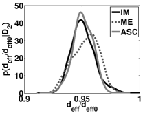
(a) Stage $2$ - $d_{eff}$

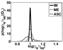
(b) Stage $2$ - $\gamma_{N}$

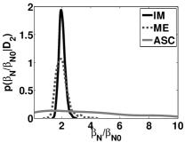
(c) Stage $2$ - $\beta_{N}$

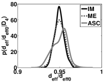
(d) Stage $4$ - $d_{eff}$

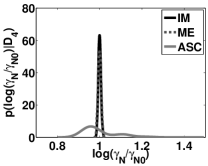
(e) Stage $4$ - $\gamma_{N}$

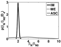
(f) Stage $4$ - $\beta_{N}$

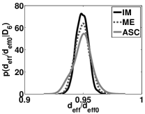
(g) Stage $6$ - $d_{eff}$

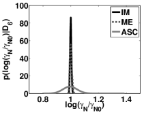
(h) Stage $6$ - $\gamma_{N}$

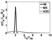
(i) Stage $6$ - $\beta_{N}$

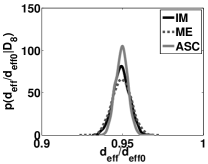
(j) Stage $8$ - $d_{eff}$

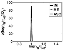
(k) Stage $8$ - $\gamma_{N}$

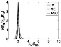
(l) Stage $8$ - $\beta_{N}$

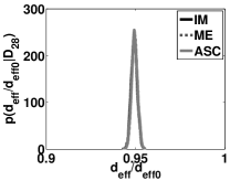
(m) Stage $28$ - $d_{eff}$

(n) Stage $28$ - $\gamma_{N}$

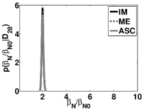
(o) Stage $28$ - $\beta_{N}$

Figure 9: Results for example $2$ (simulated data). Marginal pdfs of model parameters given by the three strategies after a selected number of experimental design stages

The marginal pdfs of the parameters at different stages are plotted in Fig.9. Note that both information theoretic approaches provide a better determination of the model parameters than the ascending sampling approach. While including all the $28$ measurements we are able to recover with good accuracy the model parameters, information maximization can provide an adequate estimate after the first two stages, followed closely by the maximum entropy sampling.

Kullback-Leibler (KL) divergence between the pdfs obtained at the current stage and the previous one is also included in order to monitor the evolution of the inference process, see Fig.8(b). The KL divergence is calculated using also a $k$NN estimator as described in the Appendix A. While the entropy quantifies how certain we are about the model parameters, the KL divergence quantifies how much information has been gained by adding the current measurement. This includes the reduction in uncertainty as well as a change in the support of the pdf. Decreasing entropy and large values of KL are indicative that the model is still learning. This is equivalent with obtaining tighter pdfs at each stage however their high probability support is changing from one stage to another. A sequence of low entropies as well as low KL divergence indicates that the learning process has slowed down and one can stop the experimental process. In this example, by thresholding the KL at $0.5$ nats, depending on the level of uncertainty, given here by the entropy, one can stop the experimental process at any stage greater than $5$. Thus for simulated data not all the $28$ measurements are needed to recover the model parameters with a given level of accuracy.

5.2 Example $3$: Study case on existing experimental measurements

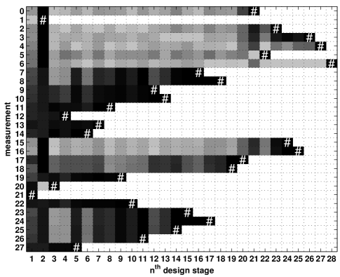
(a) IM: Relative mutual information

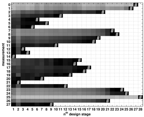
(b) ME: Relative entropy

Figure 11: Results for example $3$ (real data). Relative expected utility for Information Maximization Sampling and Maximum Entropy Sampling. Darker shadings indicate large expected utilities (mutual information for IM or entropy for ME) relative to all available scenarios within a design stage. The $\#$ sign indicates which scenario has been selected at a given stage. Previously selected scenarios are excluded from subsequent analysis which is indicated here by white cells.

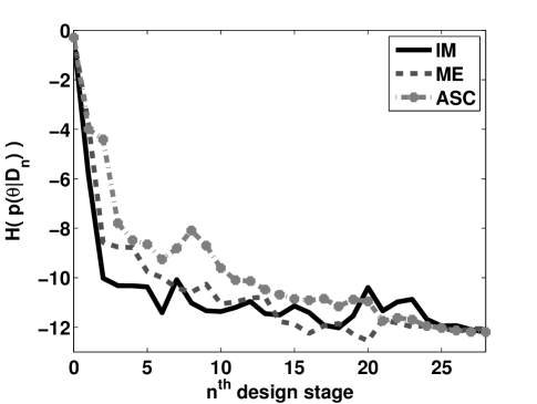
(a) Entropy

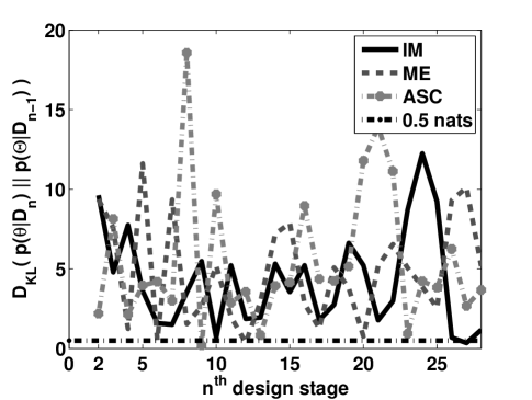
(b) Kullback Leibler divergence

Figure 13: Results for example $3$ (real data). The evolution of the entropy and the KL divergence given the posterior distributions yielded by the three strategies for experimental design: IM - Information Maximization Sampling, ME - Maximum Entropy Sampling and ASC - Ascending Sampling

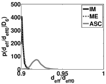
(a) Stage $6$ - $d_{eff}$

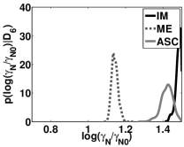
(b) Stage $6$ - $\gamma_{N}$

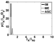
(c) Stage $6$ - $\beta_{N}$

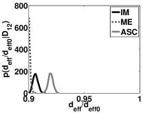
(d) Stage $12$ - $d_{eff}$

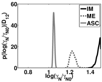
(e) Stage $12$ - $\gamma_{N}$

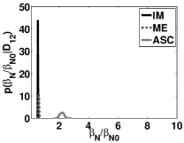
(f) Stage $12$ - $\beta_{N}$

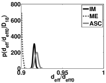
(g) Stage $18$ - $d_{eff}$

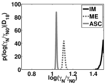
(h) Stage $18$ - $\gamma_{N}$

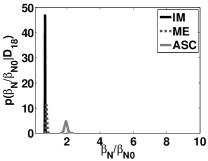
(i) Stage $18$ - $\beta_{N}$

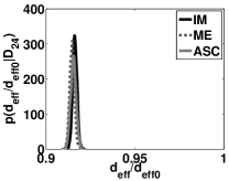
(j) Stage $24$ - $d_{eff}$

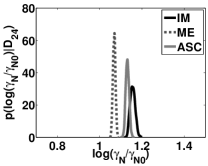
(k) Stage $24$ - $\gamma_{N}$

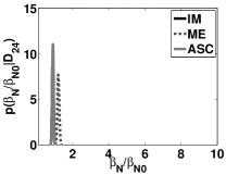
(l) Stage $24$ - $\beta_{N}$

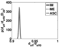
(m) Stage $28$ - $d_{eff}$

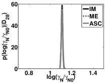
(n) Stage $28$ - $\gamma_{N}$

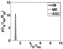
(o) Stage $28$ - $\beta_{N}$

Figure 14: Results for example $3$ (real data). Marginal pdfs of model parameters given by the three strategies after a selected number of experimental design stages

The same analysis as in the previous example is now carried on real experimental data as provided in Zhang et al. (2009). As in the simulated measurement case, both the information theoretic approaches give design sequences which start with high flow designs. See Table 5 for the corresponding design sequences or Fig. 11 for the relative expected utility corresponding to the two information theoretic strategies at each design stage. The profile of the uncertainty reduction showed in Fig.13(a) is similar with the one in Fig.8(a). However, the same cannot be said about the KL divergence plotted in Fig.13(b). No matter which design strategy is used, each subsequent measurement brings new information which moves the high probability support of the pdf from one stage to another, see Fig.14 for marginal pdfs at different design stages. As mentioned in the previous section, the model discrepancy is assumed to be Gaussian and thus in this case the likelihood function has nonzero tails. Given that the prior is uniform, the subsequent posterior pdfs will have nonzero tails over the support of the prior.

When compared with the simulated data, this behavior is indicative of conflicting information between experimental measurements and model predictions. In this case the posterior distribution asserts that the high probability support of both the prior and the data are highly implausible, for more information see O’Hagan and Forster (2004). When dealing with real data this is not unexpected given that most of the time we have model error or some of the measurements are not self-consistent. In other words, either different biases exist in the measurements or the model along with the probabilistic assumptions have limited explanatory power of the real phenomenon, or both model errors and corrupted measurements can exist at the same time. In such situations, the experimental process should be stopped after a pre-determined number of experiments to find the cause of the disagreement. While one can use a more direct way to check for this disagreement, the authors believe that using the KL divergence in this settings can provide another useful tool for model calibration diagnostics.

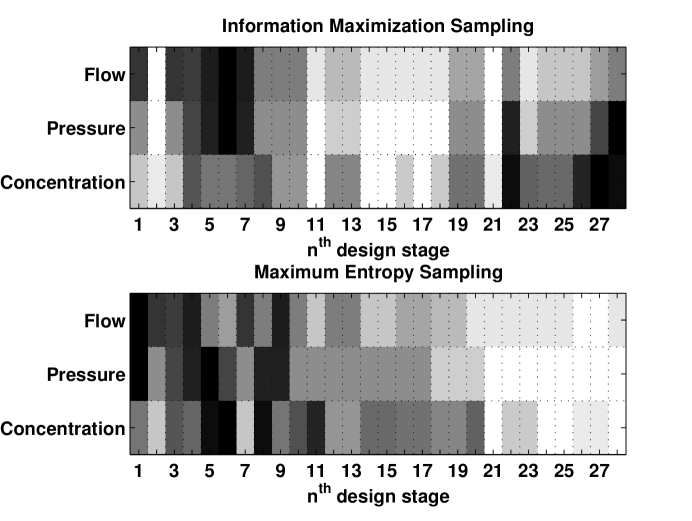
Figure 12: Results for example $3$ (real data). Graphical representation for the inflow conditions selected by the two information theoretic strategies. Darker shadings indicate large inflow conditions such as flow, pressure, and concentration.

Generally speaking, the order of measurement sequence picked by ME sampling is very close to one with the simulated data case. In other words, it picks the scenario based on the large values of either $F_{N_{2},in}$, $P_{1}$, $\mathcal{X}_{N,1}$, see Fig.12. However, IM sampling picks the experimental scenarios in a slightly different way from ones with the simulated data. For example, with the real data, IM sampling prefers the large values of inflow conditions in the early stage and does not alternatively pick different scenarios until 10^th design stage. Note 1^st measurement is selected at the second stage, however the choice of 0^th measurement is further delayed.

As mentioned above, the large values of the inflow scenario parameters are more informative due to the abundance of nitrogen atoms at the surface of the sample. However, when the real experimental data is used, this kind of data can be problematic because the physical model error and experimental uncertainty tend to be magnified in such a condition.

In Fig. 14, the pdfs of $d_{eff}$ from ME sampling stay close to the lower bound until 24^th design stage. However, the pdfs from IM sampling start to shift toward the final estimate earlier (say, after it considers 26^th measurement that has a quite small volumetric flow rate). This explains why the sampling in ascending order considering 0^th and 1^st measurements first does the better job for this parameter. For the other parameters, $\gamma_{N}$ and $\beta_{N}$, the large values of the inflow scenario parameters are preferable for getting more information due to enhancement of the chemical reactions. In the middle column of Fig. 14, the posterior pdfs of $\gamma_{N}$ from IM sampling and ME sampling appreciably varies from Stage 6 (Fig. 14(b) to Stage 12 (Fig. 14(e)).

This can be partially understood by the experimental data uncertainties related to $13^{th}$ measurement and 27^th measurement. The authors recognize these measurements are problematic and probably bring quite different information on this parameter. The scenarios of these experiments are almost identical. Nevertheless, the observed N-atom concentration is quite different (i.e., $\chi_{N,13}/\chi_{N,27}\approx 1.6$). As a result, the measurements of the mass loss that are used for calibration significantly differ each other. In fact, the local peaks seen in Fig. 13(a) at 9^th design stage from ME sampling and at 7^th design stage from IM sampling corresponds to these experiments. Moreover, the knurling feather seen in Fig. 13(b) appears to be related to some inconsistency in the experimental measurement. For example, for ME sampling, the first peak around 4^th and 5^th design stage are related to 13^th and 6^th measurements. The problem can be substantiated by a simple analysis as it follows. From Eq. (26), we get the following relationship in an approximate manner:

$$\Delta M_{C}\approx\Delta t\bar{C}_{N}\approx\Delta t\overline{P\chi}_{N},$$ (27)

where $\bar{\ast}$ is the averaged value along the sample and $\chi_{N}$ is the mole fraction ($=C_{N}RT/P$). Using the linear interpolation for the pressure and concentration, we can roughly estimate $\bar{\chi}_{N}$ and $\bar{P}$ by averaging the experimental measurements of $P$ and $\chi$ at two measurement locations. The estimated ratio of the mass loss for these experiment by Eq. (27) is given by $\Delta M^{\prime}_{C,6}/\Delta M"_{C,13}\approx 0.9$. This is significantly different from the actual measurement, $0.7$. The same kind of analysis explains the first peak appearing at 3^rd and 4^th design stage, corresponding to 20^th and 12^th measurements, for IM sampling. ($\Delta M^{\prime}_{C,20}/\Delta M"_{C,12}\approx 0.35$ that is much larger than the measurement, $0.18$). These simple analysis illustrates different experimental data provide the model with different information. As a consequence, Fig. 13(b) is significantly different from Fig. 8(b) where the simulated data is perfectly consistent with the model itself.

6 Conclusions

In this paper the experimental design problem is formulated in the Bayesian framework, and it is shown to be equivalent with an information theoretic sensitivity analysis between model parameters and observables. The optimal design selected by the information maximization sampling is the one which provides the highest statistical dependence between the two random variables. The statistical dependence is quantified using mutual information which is approximated in this paper using a $k$ nearest neighbor estimator. Theoretically the information maximization sampling is more general than the maximum entropy sampling and more efficient than random sampling.

The entropy and Kullback-Leibler information metrics are used to monitor the learning process. A decreasing trend in entropy is indicative that the uncertainty in model parameters is reduced by assimilating each additional measurement. The information gain brought by each measurement is quantified by the Kullback-Leibler divergence. Large values are indicative that the model is still learning. A large divergence between subsequent posterior distributions might be explained by a large uncertainty reduction or the existence of conflicting information between model predictions and measurements. When the trend in the Kullback-Leibler divergence is decreasing one can stop the experimental process given a level of accuracy, otherwise one may still choose to stop the experimental process to check the formulation of the model, the probabilistic assumptions and/or analyze the collected measurements to find potential outliers.

Appendix A: Estimating the Kullback-Leibler divergence using $k$NN

Similar with the entropy and mutual information, the approximation of the Kullback-Leibler divergence is based on a $k$ nearest neighbor approach as proposed in Wang et al. (2006).

$$D_{KL}(p(x|D_{n})||p(x|D_{n-1})\approx\frac{d_{X}}{N_{n}}\sum_{i=1}^{N_{n}}\log\frac{\nu_{n-1}(i)}{\rho_{n}(i)}+\log\frac{N_{n-1}}{N_{n}-1}$$ (28)

where $d_{X}$ is the dimensionality of the random variable $X$, $N_{n}$ and $N_{n-1}$ give the number of samples $\{X_{n}^{i}|i=1,\ldots,N_{n}\}\sim p(x|D_{n})$ and $\{X_{n-1}^{j}|j=1,\ldots,N_{n-1}\}\sim p(x|D_{n-1})$ respectively, and the two distances $\nu_{n-1}(i)$ and $\rho_{n}(i)$ are defined as follows:

$$\rho_{n}(i) = \min_{j=1\ldots N_{n},j\neq i}\|X_{n}^{i}-X_{n}^{j}\|_{\infty}$$ (29)

$$\nu_{n-1}(i) = \min_{j=1\ldots N_{n-1}}\|X_{n}^{i}-X_{n-1}^{j}\|_{\infty}$$ (30)

Appendix B: Information-theoretic sensitivity analysis

Mutual information is a convenient way to quantify the statistical dependence between two random variables, $X_{1}$ and $X_{2}$:

$$I(X_{1},X_{2})=\int f(x_{1},x_{2})\log\frac{f(x_{1},x_{2})}{f_{X_{1}}(x_{1})f_{X_{2}}(x_{2})}\mathrm{d}x_{1}\mathrm{d}x_{2}$$ (31)

A more formal relation between statistical dependence and mutual information can be shown with the help of copula functions as presented in Calsaverini and Vicente (2009), and included here for completeness. Sklar (1959) proved that the joint distribution of two random variables, $F(x_{1},x_{2})$, can be represented using a copula function, $C:[0,1]^{2}\rightarrow[0,1]$, and the marginals distributions, $F_{X_{i}}$:

$$F(x_{1},x_{2})=C(F_{X_{1}}(x_{1}),F_{X_{2}}(x_{2}))$$ (32)

Given that $F_{X_{1}}$ and $F_{X_{2}}$ are continuous, then $F_{X_{1}}(X_{1})$ and $F_{X_{2}}(X_{2})$ are two uniformly distributed random variables. Thus, the copula function can be regarded as a joint cumulative distribution of two uniformly distributed random variables. It separates the study of the dependence between random variables and their marginal distributions. By denoting $u_{i}=F_{X_{i}}(x_{i})$, Eq. (32) can be written as follows:

$$F(F_{X_{1}}^{-1}(u_{1}),F_{X_{2}}^{-1}(u_{2}))=C(u_{1},u_{2})$$ (33)

Assuming that the densities $f_{X_{i}}$ exist, then the joint probability density function is given by:

$$f(x_{1},x_{2}) = \frac{\partial^{2}}{\partial x_{1}\partial x_{2}}F(x_{1},x_{2})$$ (34)

$$= c(F_{X_{1}}(x_{1}),F_{X_{2}}(x_{2}))f_{X_{1}}(x_{1})f_{X_{2}}(x_{2})$$

where $c(F_{X_{1}}(x_{1}),F_{X_{2}}(x_{2}))=\frac{\partial^{2}}{\partial x_{1}\partial x_{2}}C(F_{X_{1}}(x_{1}),F_{X_{2}}(x_{2}))$ is the copula density.

By substituting Eq. (34) in Eq. (31), and using that $u_{i}=F_{X_{i}}(x_{i})$, the mutual information can be rewritten in terms of copula density function.

$$I(X_{1},X_{2}) = \int c(F_{X_{1}}(x_{1}),F_{X_{2}}(x_{2}))f_{X_{1}}(x_{1})f_{X_{2}}(x_{2})\log c(F_{X_{1}}(x_{1}),F_{X_{2}}(x_{2}))\mathrm{d}x_{1}\mathrm{d}x_{2}$$ (35)

$$= \int c(u_{1},u_{2})\log c(u_{1},u_{2})\mathrm{d}u_{1}\mathrm{d}u_{2}$$

Eq. (35) reveals that mutual information is the negative copula entropy. Thus it does not depend on the marginal distributions, it only quantifies the dependence between the random variables which is contained in the copula function. This has been pointed out in literature in Calsaverini and Vicente (2009).

Sample Size $\rightarrow$			$500$			$1,000$			$2,000$
Dimensionality			$k$NN			$k$NN			$k$NN
dim$(\mathbf{X},\mathbf{Y})$	dim$(\mathbf{X})$	dim$(\mathbf{Y})$	$3$	$6$	$9$	$3$	$6$	$9$	$3$	$6$	$9$
$2$	$1$	$1$	$16\%$	$10\%$	$~{}8\%$	$11\%$	$~{}7\%$	$~{}5\%$	$~{}8\%$	$~{}5\%$	$~{}3\%$
$3$	$2$	$1$	$21\%$	$13\%$	$11\%$	$16\%$	$~{}9\%$	$~{}7\%$	$12\%$	$~{}7\%$	$~{}5\%$
$4$	$2$	$2$	$15\%$	$11\%$	$11\%$	$10\%$	$~{}7\%$	$~{}6\%$	$~{}7\%$	$~{}5\%$	$~{}4\%$
$5$	$3$	$2$	$18\%$	$14\%$	$13\%$	$13\%$	$~{}9\%$	$~{}9\%$	$~{}9\%$	$~{}6\%$	$~{}9\%$

Table 1: Absolute Relative Error for MI averaged over $1000$ trial runs

Strategy	Sequence
Repeated measurements not allowed
ME Sampling	$10~{}~{}1~{}~{}9~{}~{}2~{}~{}3~{}~{}8~{}~{}5~{}~{}7~{}~{}4~{}~{}6$
IM Sampling	$~{}1~{}10~{}~{}9~{}~{}2~{}~{}3~{}~{}8~{}~{}7~{}~{}4~{}~{}6~{}~{}5$
RND Sampling	$~{}6~{}10~{}~{}3~{}~{}1~{}~{}5~{}~{}9~{}~{}8~{}~{}2~{}~{}4~{}~{}7$
Repeated measurements allowed
ME Sampling	$10~{}~{}1~{}10~{}~{}1~{}~{}1~{}10~{}10~{}~{}1~{}~{}1~{}~{}1$
IM Sampling	$~{}1~{}10~{}~{}1~{}10~{}10~{}~{}1~{}10~{}10~{}~{}1~{}~{}1$

Table 2: Results for example $1$, the additive noise case. Design sequences yielded by the three strategies for one particular Monte Carlo run

Strategy	Sequence
Repeated measurements not allowed
ME Sampling	$~{}5~{}~{}6~{}~{}7~{}~{}4~{}~{}1~{}~{}3~{}~{}8~{}~{}9~{}~{}2~{}10$
IM Sampling	$~{}1~{}10~{}~{}9~{}~{}7~{}~{}2~{}~{}8~{}~{}4~{}~{}3~{}~{}5~{}~{}6$
RND Sampling	$~{}6~{}~{}1~{}~{}8~{}~{}5~{}10~{}~{}9~{}~{}4~{}~{}2~{}~{}3~{}~{}7$
Repeated measurements allowed
ME Sampling	$~{}5~{}~{}6~{}~{}6~{}~{}5~{}~{}5~{}~{}5~{}~{}6~{}~{}5~{}~{}6~{}~{}5$
IM Sampling	$~{}1~{}10~{}~{}1~{}10~{}10~{}~{}1~{}~{}1~{}~{}1~{}~{}1~{}10$

Table 3: Results for example $1$, the multiplicative noise case. Design sequences yielded by the three strategies for one particular Monte Carlo run

Strategy	Sequence
ME Sampling	$14~{}21~{}6~{}20~{}13~{}12~{}27~{}19~{}5~{}11~{}22~{}4~{}18~{}17~{}10~{}3~{}9~{}16~{}15~{}26~{}2~{}7~{}23~{}8~{}24~{}25~{}1~{}0$
IM Sampling	$21~{}5~{}20~{}0~{}1~{}13~{}27~{}14~{}2~{}12~{}15~{}16~{}11~{}22~{}19~{}9~{}10~{}3~{}4~{}6~{}26~{}25~{}23~{}7~{}8~{}24~{}18~{}17$
ASC Sampling	$0~{}1~{}2~{}3~{}4~{}5~{}6~{}7~{}8~{}9~{}10~{}11~{}12~{}13~{}14~{}15~{}16~{}17~{}18~{}19~{}20~{}21~{}22~{}23~{}24~{}25~{}26~{}27$

Table 4: Results for example $2$ (simulated data). Design sequences yielded by the three strategies.

Strategy	Sequence
ME Sampling	$14~{}21~{}12~{}13~{}6~{}4~{}20~{}5~{}27~{}11~{}3~{}22~{}19~{}16~{}15~{}18~{}17~{}10~{}9~{}2~{}26~{}7~{}8~{}23~{}24~{}1~{}0~{}25$
IM Sampling	$21~{}1~{}20~{}12~{}27~{}14~{}13~{}11~{}19~{}22~{}26~{}9~{}10~{}25~{}23~{}7~{}24~{}8~{}18~{}17~{}0~{}5~{}2~{}15~{}16~{}3~{}4~{}6$
ASC Sampling	$0~{}1~{}2~{}3~{}4~{}5~{}6~{}7~{}8~{}9~{}10~{}11~{}12~{}13~{}14~{}15~{}16~{}17~{}18~{}19~{}20~{}21~{}22~{}23~{}24~{}25~{}26~{}27$

Table 5: Results for example $3$ (real data). Design sequences yielded by the three strategies.

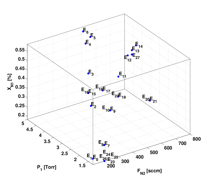
Figure 5: Results for example $2$ (simulated data). 3D plot for inflow scenarios used in Ref. Zhang et al. (2009).

References

- Chaloner and Verdinelli (1995) K. Chaloner, I. Verdinelli, Bayesian Experimental Design: A Review, Statistical Science 10(3) (1995) 273–304.
- Shannon (1948) C. Shannon, A Mathematical Theory of Communication, Bell System Technical Journal 27 (July, October, 1948) 379–423, 623–656.
- Lindley (1956) D. V. Lindley, On a Measure of the Information Provided by an Experiment, Ann. Math. Statist. 27(4) (1956) 986–1005.
- Fedorov (1972) V. Fedorov, Theory of optimal experiments, Academic press New York and London, 1972.
- Loredo and Chernoff (2003) T. Loredo, D. Chernoff, Bayesian Adaptive Exploration, Statistical Challenges in Astronomy (2003) 57–70.
- DasGupta (1995) A. DasGupta, Review of optimal Bayes designs, Tech. Rep., Purdue University, 1995.
- Muller (1999) P. Muller, Bayesian Statistics 6, chap. Simulation-based optimal design, Oxford University Press, 459–474, 1999.
- Sebastiani and Wynn (1997) P. Sebastiani, H. P. Wynn, Bayesian Experimental Design and Shannon Information, in: Bayesian Statistical Science, American Statistical Association, 176–181, 1997.
- Shewry and Wynn (1987) M. Shewry, H. Wynn, Maximum entropy sampling, Journal of Applied Statistics (1987) 165–170.
- Farhang-Mehr and Azarm (2002) A. Farhang-Mehr, S. Azarm, A sequential information-theoretic approach to design of computer experiments, in: AIAA, Atlanta, Georgia, AIAA 2002–5571, 2002.
- Calsaverini and Vicente (2009) R. Calsaverini, R. Vicente, An information-theoretic approach to statistical dependence: Copula information, EPL (Europhysics Letters) 88 (6) (2009) 68003.
- Cheung and Beck (2009) S. H. Cheung, J. L. Beck, New Bayesian Updating Methodology for Model Validation and Robust Predictions of a Target System based on Hierarchical Subsystem Tests., Computer Methods in Applied Mechanics and Engineering Accepted for publication.
- Kraskov et al. (2004) A. Kraskov, H. Stogbauer, P. Grassberger, Estimating mutual information, Physical Review E 69 (6) (2004) 066138.
- Kozachenko and Leonenko (1987) L. F. Kozachenko, N. N. Leonenko, Sample Estimate of the Entropy of a Random Vector, Problems of Information Transmission 23(2) (1987) 9–16.
- Guest and Curtis (2009) T. Guest, A. Curtis, Iteratively constructive sequential design of experiments and surveys with nonlinear parameter-data relationships, Journal of Geophysical Research 114 (2009) B04307.
- Paninski (2005) L. Paninski, Asymptotic theory of information-theoretic experimental design, Neural Computation 17 (2005) 1480–1507.
- Clyde et al. (1996) M. Clyde, P. Muller, G. Parmigiani, Bayesian Biostatistics, chap. Inference and Design Strategies for a Hierarchical Logistic Regression Model, Dekker, New York, 297–320, 1996.
- Chung and Haber (2011) M. Chung, E. Haber, Experimental design in biological systems, in revision at SIAM Journal on Control and Optimization, 2011 .
- Horesh et al. (2011) L. Horesh, E. Haber, L. Tenorio, Large-Scale Inverse Problems and Quantification of Uncertainty, chap. Optimal Experimental Design for the Large-Scale Nonlinear Ill-posed Problem of Impedance Imaging, Wiley, 273–290, 2011.
- Tucker (2008) M. A. A. Tucker, Application of Design of Experiments to Flight Test: A Case Study, in: AIAA, Los Angeles, California, 2008–847, 2008.
- Curtis and Maurer (2000) A. Curtis, H. Maurer, Optimizing the design of geophysical experiments: Is it worthwhile?, EOS, Trans. A,. Geophys. Un. 81 (20) (2000) 224–225.
- Zhang et al. (2009) L. Zhang, D. A. Pejakovic, J. Marschall, D. G. Fletcher, Laboratory Investigation of Active Carbon Nitridation by Atomic Nitrogen, AIAA Paper 2009-4251, AIAA, 2009.
- Park and Bogdanoff (2006) C. Park, D. W. Bogdanoff, Shock-Tube Measurement of Nitridation Coefficient of Solid Carbon, Journal of Thermophysics and Heat Transfer 20 (2006) 487–492.
- Goldstein (1964) H. W. Goldstein, The Reaction of Active Nitrogen with Graphite, Journal of Physical Chemistry 68 (1) (1964) 39–42.
- Suzuki et al. (2008) T. Suzuki, K. Fujita, K. Ando, T. Sakai, Experimental Study of Graphite Ablation in Nitrogen Flow, Journal of Thermophysics and Heat Transfer 22 (2008) 382–389.
- Prudencio and Schulz (2011) E. E. Prudencio, K. W. Schulz, The Parallel C++ Statistical Library ‘QUESO’: Quantification of Uncertainty for Estimation, Simulation and Optimization, Submitted to IEEE IPDPS .
- Cheung and Beck (2008) S. H. Cheung, J. L. Beck, New Bayesian updating methodology for model validation and robust predictions based on data from hierarchical subsystem tests, EERL Report No.2008-04, California Institute of Technology., 2008.
- Cover and Thomas (1991) T. Cover, J. Thomas, Elements of Information Theory, New York: Wiley, 1991.
- Sebastini and Wynn (2000) P. Sebastini, H. P. Wynn, Maximum entropy sampling and optimal Bayesian experimental design, J. R. Statist. Soc. B 62, Part 1 (2000) 145–157.
- Khan et al. (2007) S. Khan, S. Bandyopadhyay, A. R. Ganguly, S. Saigal, Relative performance of mutual information estimation methods for quantifying the dependence among short and noisy data, Physical Review E 76 (2007) 026209.
- O’Hagan and Forster (2004) A. O’Hagan, J. Forster, Kendall’s Advanced Theory of Statistics. Bayesian Inference, v.2B, Oxford University Press Inc, New York, 79–80, 2004.
- Wang et al. (2006) Q. Wang, S. Kulkarni, S. Verdu, A Nearest-Neighbor Approach to Estimating Divergence between Continuous Random Vectors, in: Information Theory, 2006 IEEE International Symposium on, 242 –246, doi:10.1109/ISIT.2006.261842, 2006.
- Sklar (1959) A. Sklar, Fonctions de repartition a n dimensions et leurs marges, Publications de l’Institut de Statistique de l’Universite de Paris, Paris 8.