Vacancy-induced spin texture in a one dimensional $S=1/2$ Heisenberg antiferromagnet

Abstract

We study the effect of a missing spin in a one dimensional $S=1/2$ antiferromagnet with nearest neighbour Heisenberg exchange $J$ and six-spin coupling $Q=4qJ$ using Quantum Monte-Carlo (QMC) and bosonization techniques. For $q<q_{c}\approx 0.04$, the system is in a quasi-long range ordered power-law antiferromagnetic phase, which gives way to a valence-bond solid state that spontaneously breaks lattice translation symmetry for $q>q_{c}$. We study the ground state spin texture $\Phi(r)=\langle G_{\uparrow}|S^{z}(r)|G_{\uparrow}\rangle$ in the the $S^{z}_{tot}=1/2$ ground state $|G_{\uparrow}rangle$ of the system with a missing spin, focusing on the alternating part $N_{z}(r)$. We find that our QMC results for $N_{z}$ at $q=q_{c}$ take on the scaling form expected from bosonization considerations, but violate scaling for $q<q_{c}$. Within the bosonization approach, such violations of scaling arise from the presence of a marginally irrelevant sine-Gordon interaction, whose effects we calculate using renormalization group (RG) improved perturbation theory. Our field-theoretical predictions are found to agree well with the QMC data for $q<q_{c}$.

I Introduction

The one-dimensional $S=1/2$ Heisenberg antiferromagnetic spin chain, with nearest-neighbour exchange couplings $J$ is perhaps the simplest important model spin system in quantum magnetism. It has not only proved useful as a theoretical model for the magnetic properties of several Mott insulating materialsexptchains ; exptchains1 ; exptchains2 ; exptchains3 , but has also been the subject of many theoretical advances such as Bethe’s original ‘Bethe Ansatz’ solution of this quantum many-body problem and later field-theoretical treatments that applied bosonization techniques to map the system to a $1+1$ dimensional bosonic field theory with a so-called ‘sine-Gordon’ action, made up of a scale invariant free-field part perturbed by a non-linear cosine interaction.Affleck_review In addition, the renormalization group (RG) analysis of the cosine interaction that perturbs the scale-invariant free-field action is a paradigmatic example of the treatment of ‘marginally irrelevant’ interactions in the neighbourhood of a well-characterized and tractable scale invariant RG fixed point.Singh_Fisher_Shankar ; Affleck_Gepner_Shultz_Ziman ; Barzykin_Affleck ; Orignac ; Diptiman ; Eggert

Such marginally irrelevant interactions can give rise to violations of scaling predictions at critical points due to the presence of logarithmic corrections that multiply the scaling answer. A well known example is the $O(N)$ critical point in four space-time dimensions.Kenna_ONmodel In some other cases, such marginally irrelevant interactions give rise to additive corrections to scaling, which vanish logarithmically slowly. The one dimensional Heisenberg chain displays both kinds of effects. For instance, gaps in the finite size spectra of the spin-half chain are known to have additive logarithmic corrections that do not affect the leading behaviourAffleck_Gepner_Shultz_Ziman , while the temperature dependence of the NMR relaxation rate $1/T_{1}$ violates scaling expectations due to the presence of an additional logarithmic factor in its temperature dependence.Sachdev

Similar logarithmic violations of scaling, arising from multiplicative logarithmic factors that multiply scaling predictions, have been argued to existSandvik ; Banerjee_Damle_Alet1 in a much less well-understood case of a two dimensional $S=1/2$ square lattice Heisenberg antiferromagnet on the verge of a continuous quantum phase transitionSenthil_etal ; Sandvik_original between the usual Neel ordered antiferromagnetic ground state and a spontaneously dimerized non-magnetic state with valence-bond order. The underlying critical non-compact CP¹ (NCCP¹) field theory that has been proposedSenthil_etal as the continuum description of this transition is not as well understood from a RG standpoint, and since the numerics themselves are also more challenging, there have been some differences in the interpretation of these results.Sandvik_Kotov_Sushkov ; Kaul

In our own recent work,Banerjee_Damle_Alet1 we have used extensive numerical computations to establish the presence of apparently logarithmic scaling violations in the impurity spin texture induced by a missing-spin defect at such a quantum critical point when the system has the usual $SU(2)$ symmetry of spin rotations, and ascribed this effect to the presence of a yet-to-be-identified marginal operator at the putative NCCP¹ critical fixed point. In contrast, the corresponding spin texture in a system at an analogous critical point with enlarged $SU(3)$ symmetrySandvik_SU3 was found to obey scaling predictions without any logarithmic violations,Banerjee_Damle_Alet2 , suggesting that the underlying NCCP² critical point describing this $SU(3)$ transition is free of such marginal operators. However, parallel work of KaulKaul argues that such marginal operators would typically not lead to violations of scaling, and finds an alternative scenario more likely. In this alternative scenario, both the $SU(2)$ and $SU(3)$ transitions are described by fixed points with a leading irrelevant operator with small scaling dimension, and the violations of scaling arise from the fact that the quantity being studied depends non-analytically on this leading irrelevant operator.

Here, we try and understand the origins of such multiplicative logarithmic corrections to impurity spin textures by using the one dimensional Heisenberg antiferromagnet as an example. On the analytical side, we work within the bosonization framework and use renormalization group (RG) improved perturbation theory to obtain predictions for the alternating part of the spin texture in this example. These predictions are compared with Quantum Monte-Carlo (QMC) results for a one-dimensional chain with nearest neighbour Heisenberg exchange $J$ and six-spin coupling $Q=4qJ$. The Hamiltonian for this ‘$JQ_{3}$ model’ is:

$$H=-J\sum_{i=0}^{N}P_{i,i+1}-Q\sum_{i}P_{i,i+1}P_{i+2,i+3}P_{i+4,i+5}$$ (1)

where $P_{ij}\equiv(\frac{1}{4}-\vec{S}_{i}\cdot\vec{S}_{j})$ is the projector to the singlet state of the two spin-half variables at sites $i$ and $j$, both $J$ and $Q$ are assumed positive, and we impose periodic boundary conditions by placing the system on a ring so that site $N+1+k$ is identified with site $k$ (the total number of spins $N+1$ is taken even).

From our QMC results, obtained using the singlet sector valence-bond projection methodSandvik_Evertz , we find that the $Q$ term drives a transition to a valence-bond solid phase at $q_{c}\approx 0.04$, so that the system is power-law Neel ordered for $q<q_{c}$, and VBS ordered for $q>q_{c}$. Unlike the more well-studied case in which such a transition is driven by next-nearest neighbour Heisenberg antiferromagnetic exchange couplings, the present $JQ_{3}$ model does not have a sign problem in standard non-zero temperature QMC calculations (as well as in the ground state projector QMC approach), and can therefore be studied at larger length scales and greater precision.

In order to explore the effects of vacancy defects, we remove the spin at site $0$ and delete all interactions that involve this spin from our Hamiltonian. Since $N$ is odd, the ground state of the chain with a missing spin is a doublet with $S_{tot}=1/2$. We focus on $|G_{\uparrow}\rangle$, the $S^{z}_{tot}=1/2$ component of this doublet, and compute the spin texture $\Phi(r)=\langle S^{z}(r)\rangle_{\uparrow}$ in this ground state for various values of $q$. This is done using a recently developed modificationBanerjee_Damle of the singlet-sector projector Quantum Monte Carlo (QMC) technique.Sandvik_Evertz . This spin texture can be decomposed as $\Phi(r)=\Phi_{u}(r)+(-1)^{r/a}N_{z}(r)$, where alternating part $N_{z}(r)$ and a uniform part $\Phi_{u}(r)$ are obtained from our numerical data by a suitable coarse-graining procedure.

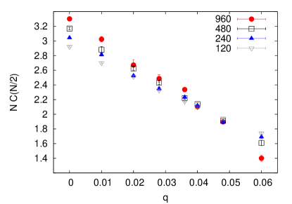
Figure 1: Spin-spin correlation function at distance $N/2$ $C(N/2)=\langle\vec{S}_{i}\cdot\vec{S}_{i+N}\rangle$ in the ground state of a periodic chain with $N$ spins, multiplied by $N$ and plotted against $q$ to serve as diagnostic of the quantum phase transition from power-law Neel order to valence-bond solid order, as discussed in the text.

These numerical results for $N_{z}(r)$ are compared to field theoretical calculations within the bosonization framework, keeping careful track of the effects of the marginal cosine interaction term using one loop RG improved perturbation theory. Our basic conclusion is that this marginal cosine interaction does indeed lead to logarithmic violations of scaling by introducing logarithmic corrections that multiply the scaling predictions for $N_{z}$ in the power-law Neel phase. Comparing these analytical predictions with our numerical results for $q<q_{c}$, we find good agreement with the data, with the strength of the log corrections being larger for $q$ further away from the critical point, and vanishing for $q=q_{c}$, as predicted by the bosonization approach.

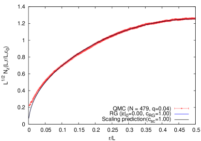
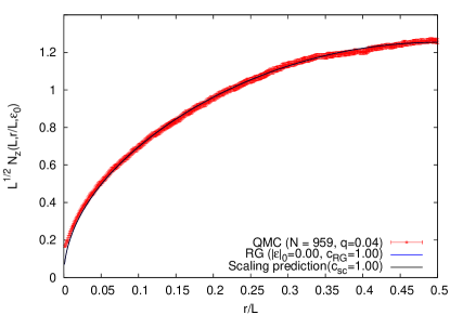
Figure 2: $L^{1/2}N_{z}(r)$ plotted versus $r/L$ (where $L=N+1$ for chains with $N=959$ and $N=479$ spins and open boundary conditions) and compared with the scaling prediction $F_{0}$ for $q=0.04$, the approximate location of the quantum critical point separating the power-law Neel phase from the VBS ordered phase in the one dimensional $JQ_{3}$ model. Note the data at both sizes fits essentially perfectly to the scaling prediction with the same prefactor $c_{sc}$. Also note that the best two-parameter fit corresponding to our RG improved perturbation theory result also gives $|\epsilon_{0}|=0$, and thus coincides with the scaling answer.

The rest of this article is organized as follows: In Section II, we first summarize our approach to the analytical calculation of the ground state spin texture induced by a missing spin, give our final predictions for the nature of the logarithmic violations of scaling, and discuss them from a somewhat more general RG standpoint. In Section III, we describe our projector QMC studies and compare the numerical data for $N_{z}$ with our analytical predictions to establish our main results. We conclude with a very brief discussion regarding the connection between our results and earlier work on the effect of vacancies on the NMR Knight shift and the spin structure factor.

II Bosonization calculation of ground state spin texture

II.1 Preliminaries

As is well-known, we may model our one dimensional magnet by the continuum effective HamiltonianAffleck_review

$$H=H_{0}+H_{1}$$ (2)

where the free field part $H_{0}$ is written as

$$H_{0}=\frac{u}{2}\int^{L}_{0}dx\left[\left(\dfrac{d\phi}{dx}\right)^{2}+\left(\dfrac{d\widetilde{\phi}}{dx}\right)^{2}\right]\;,$$ (3)

and the interaction term $H_{1}$ reads

$$H_{1}=-\frac{u\epsilon_{0}}{r_{0}^{2}}\int^{L}_{0}dx\cos\left(\frac{2\phi(x)}{R}\right)\;;$$ (4)

here $r_{0}$ is an ultraviolet regulator defined precisely later and

$$\frac{1}{2\pi R^{2}}=1-\pi\epsilon_{0}\;.$$ (5)

The last constraint that relates $R$ to the bare coupling constant $\epsilon_{0}$ at scale $r_{0}$ arises from the $SU(2)$ spin invariance of the underlying microscopic theory.Orignac The well-known Kosterlitz-Thouless renormalization group theoryJose_Kadanoff_Kirkpatrick_Nelson applied to the present SU(2) symmetric case yields the flow equation

$$\dfrac{d\epsilon}{d\log L)}=\beta_{\epsilon}(\epsilon(L))$$ (6)

with the one loop expression for the beta function being given byBarzykin_Affleck

$$\beta_{\epsilon}(\epsilon(L))=2\pi\epsilon^{2}(L)-\frac{1}{2}(2\pi)^{2})\epsilon^{3}(L)\;.$$ (7)

This equation can be solved to obtain the running coupling constant $\epsilon(L)$ at scale $L$ asBarzykin_Affleck

$$\frac{1}{\epsilon(L)}-\frac{1}{\epsilon_{0}}=-2\pi\left\{\log\left(\frac{L}{r_{0}}\right)+\frac{1}{2}\log\left(\log\left(\frac{L}{r_{0}}\right)\right)\right\}+O(1)$$ (8)

Note that $\epsilon_{0}$ is negative in the power-law ordered antiferromagnetic phase in the present sign convention.

Within this bosonized formulation, the operator $S^{z}(r)$ at site $r=ja$ is represented asFurusaki_Hirahara

$$S^{z}(r)=\frac{a}{2\pi R}\frac{d\phi}{dr}+\frac{\mathcal{A}}{\sqrt{r_{0}}}(-1)^{\frac{r}{a}}\sin\left(\frac{\phi(r)}{R}\right)\;.$$ (9)

Here, the coefficient of the uniform part is fixed by $SU(2)$ invariance while the coefficient of the alternating part is sensitive to microscopic details: $\mathcal{A}=\sqrt{a}c$ where $a$ is lattice spacing of lattice model and $c$ is a pure number that depends on the microscopic Hamiltonian.

Finally, we also recall that the 1-point function $S=\langle\frac{1}{\sqrt{r_{0}}}\sin\left(\frac{\phi(r)}{R}\right)\rangle_{\uparrow}$ of the operator $\frac{1}{\sqrt{r_{0}}}\sin\left(\frac{\phi(r)}{R}\right)$ can be thought of as a function of $L$ and the running coupling $\epsilon(L)$ for fixed bare coupling $\epsilon_{0}$ and fixed $r/L$. Thought of in this way, it obeys the Callan-Symanzik type equationBarzykin_Affleck

$$\left(\frac{\partial}{\partial lnL}+\beta_{\epsilon}(\epsilon)\frac{\partial}{\partial\epsilon}+\gamma(\epsilon)\right)S\left(L,\epsilon(L)\right|\epsilon_{0},\frac{r}{L})=0.$$ (10)

with the anomalous dimension having the expansion

$$\gamma(\epsilon)=\frac{1}{2}+\left(\frac{\pi}{2}\right)\epsilon(L)$$ (11)

in terms of the running coupling $\epsilon$. As is well-known, this can be solved to leading order in $\epsilon(L)$ to give the following scaling law for $S$

$$S\cong\frac{F_{0}}{\sqrt{L}}\left(\frac{\epsilon_{0}}{\epsilon(L)}\right)^{\frac{1}{4}}(1+\epsilon(L)R)\;,$$ (12)

where $F_{0}\left(\frac{r}{L}\right)$ and $R\left(\frac{r}{L}\right)$ are some functions of the ratio $\frac{r}{L}$ and the key point about this formal expression for $S$ is that all dependence on the ultraviolet regulator $r_{0}$ has been traded in for a dependence on $\epsilon(L)$, the running coupling at scale $L$ for a flow that starts with bare coupling $\epsilon_{0}$ at scale $r_{0}$.

II.2 Overview

With these preliminaries out of the way, we now outline the strategy used below to calculate the alternating part of $\langle S^{z}(r)\rangle_{\uparrow}$. The basic idea is to begin by calculating the result for this alternating part using the bosonized part of the alternating spin density and bare perturbation theory to first order in $\epsilon_{0}$ for a finite system of length $L$. As we shall see below, this bare perturbation theory result will turn out to depend logarithmically on the value of the ultraviolet cutoff $r_{0}$ via a logarithmic ultraviolet divergence arising from a first order perturbation theory contribution proportional to $\epsilon_{0}\log\frac{L}{r_{0}}$. This logarithmic divergence makes bare perturbation theory suspect, since a notionally small ${\mathcal{O}}(\epsilon_{0})$ correction turns out to have a logarithmically diverging coefficient.

To extract useful information from the bare perturbation theory, it is therefore necessary to appeal to the Callan-Symanzik equation for the one point function $S$, and use the fact that $S$ is expected to have the general form

$$S\cong\frac{F_{0}}{\sqrt{L}}\left(\frac{\epsilon_{0}}{\epsilon(L)}\right)^{\frac{1}{4}}(1+\epsilon(L)R)\;,$$ (13)

as noted earlier. In order to make contact with our bare perturbation theory result, we expand this renormalization group prediction to first order in the bare coupling constant:

$$S=\frac{F_{0}\left(\frac{r}{L}\right)}{\sqrt{L}}\left(1-\frac{\pi}{2}\epsilon_{0}\log\frac{L}{r_{0}}+....\right)\left(1+\epsilon_{0}R(\frac{r}{L})+....\right)$$

$$\cong\frac{F_{0}(\frac{r}{L})}{\sqrt{L}}\left(1-\frac{\pi}{2}\epsilon_{0}\log\frac{L}{r_{0}}+\epsilon_{0}R(\frac{r}{L})+....\right).$$ (14)

By comparing with the result of our first order perturbation theory in $\epsilon_{0}$, it becomes possible to fix the functions $F_{0}$ and $R$. This strategy gives us the one-loop RG improved result for the alternating part of $\langle S^{z}(r)\rangle_{\uparrow}$

$$N_{z}(r)=c\sqrt{a}\frac{F_{0}}{\sqrt{L}}\left(\frac{\epsilon_{0}}{\epsilon(L)}\right)^{\frac{1}{4}}(1+\epsilon(L)R)\;,$$ (15)

with

$$F_{0}(\frac{r}{L})=-\sqrt{\frac{\pi\sin\theta_{r}}{2}}\;,$$ (16)

and

$$R(\frac{r}{L})=\frac{\pi}{2}\log\frac{2\pi}{\sin\theta_{r}}+2\left(\int_{0}^{\theta_{r}}+\int_{0}^{\pi-\theta_{r}}\right)\phi\cot\phi d\phi\;,$$ (17)

with $\theta_{r}\equiv\frac{\pi r}{L}$.

In order to cast this expression into an explicitly useful form for comparison with numerical results on a chain of $N$ sites with lattice spacing $a$, we rewrite the prefactor as

$$\left(\frac{\epsilon_{0}}{\epsilon(L)}\right)^{\frac{1}{4}}\approx$$

$$\left(1+2\pi|\epsilon_{0}|\left\{\log\left(\frac{L}{r_{0}}\right)+\frac{1}{2}\log\left(\log\left(\frac{L}{r_{0}}\right)\right)\right\}\right)^{1/4}\;,$$

express $\epsilon(L)$ as

$$\epsilon(L)=-\frac{|\epsilon_{0}|}{1+2\pi|\epsilon_{0}|\left\{\log\left(\frac{L}{r_{0}}\right)+\frac{1}{2}\log\left(\log\left(\frac{L}{r_{0}}\right)\right)\right\}}\;,$$ (19)

choose the short-distance cutoff as $r_{0}=a$, and set the length $L$ to $L=(N+1)a$ (see subsection II.3 below). Eqns (15),(16), (17) with these inputs constitutes a theoretical prediction with two free parameters (the overall amplitude $c$, and the bare coupling $\epsilon_{0}$ at the lattice scale), and we find below that this provides an extremely good two-parameter fit of our numerical data in the power-law ordered antiferromagnetic phase of the one dimensional $JQ_{3}$ model. In addition, the spin texture at $q=q_{c}$, the critical end-point of this power-law ordered Neel phase, fits extremely well to the scaling function $F_{0}$, to which the more general prediction reduces when $\epsilon_{0}=0$.

What do these results tell us about the possible origins of such multiplicative logarithmic corrections to spin textures at other critical points? To explore this, let us consider the same calculation of the spin texture, but at a different critical point with an irrelevant coupling $g$ with small scaling dimension $\alpha$. In other words, we assume that $\beta(g)=-\alpha g+\dots$ with $\alpha$ small and positive, and $\gamma(g)=\delta_{0}+\delta_{1}g+\dots$. In this case, the Callan-Symanzik equation would predict that $N_{z}$ satisfy the scaling law

$$N_{z}(\vec{r})=\exp\left(-\int_{g_{0}}^{g(L)}\frac{\gamma(g)}{\beta(g)}dg\right)F\left(\frac{\vec{r}}{L},g(L)\right)$$ (20)

for some function $F$ (that needs a more detailed analysis to determine). Using the postulated form of the $\beta$ and $\gamma$ functions, one can therefore conclude

$$N_{z}(\vec{r})=\frac{{\cal C}}{L^{\delta_{0}}}F\left(\frac{\vec{r}}{L},g_{0}/L^{\alpha}\right)$$ (21)

Thus, if the critical point in question has no marginal operators, the spin texture will quite generally obey scaling as long as the scaling function $F(x,y)$ does not diverge as $y\rightarrow 0$. Conversely, if the critical point in question has a marginal operator, scaling will always be violated by multiplicative logarithmic factors even if the scaling function $F(x,y)$ is perfectly analytic and well-defined in the $y\rightarrow 0$ limit. Indeed, in this marginal case, the only way of evading a multiplicative logarithmic correction would be to “arrange” for the $y\rightarrow 0$ limit of the scaling function $F(x,y)$ to have exactly the “right” kind of singularity needed to cancel the effects of the multiplicative logarithmic correction coming from the exponential prefactor. One may therefore conclude that unless the scaling function has a particularly “fine-tuned” form, scaling predictions for $N_{z}$ will be generically violated by multiplicative logarithmic corrections in the presence of a marginal operator. Conversely, irrelevant operators can lead to violations of scaling only if the scaling function has a divergence as this operator renormalizes to zero.

II.3 Details

When a missing-spin defect is introduced into a periodic spin chain of $N+1$ sites, it converts the system into a spin chain of $N$ spins obeying open boundary conditions. These open boundary conditions can be modeled by refering back to the original periodic system and requiring that the spin density is constrained to go to zero at the missing site. As is well known,Furusaki_Hirahara ; Eggert_Affleck this boundary condition can be incorporated by expanding the bosonic field $\phi$ in terms of bosonic normal modes as follows:

$$\phi(r) = \pi R+\frac{q_{0}}{L}r+\sum_{n=1}^{\infty}\frac{\sin\left(\frac{n\pi r}{L}\right)(a_{n}+a_{n}^{\dagger})}{\sqrt{\pi n}}$$ (22)

$$\widetilde{\phi}(r) = \widetilde{\phi}_{0}+i\sum_{n=1}^{\infty}\frac{\cos\left(\frac{n\pi r}{L}\right)(a_{n}-a_{n}^{\dagger})}{\sqrt{\pi n}}\;.$$

Here, the non zero bosonic commutation relations are $\left[\widetilde{\phi}(0),q_{0}\right]=i$,$\left[a_{m},a_{n}^{\dagger}\right]=\delta_{mn}$, $H_{0}$ can be written (apart from an (infinite) constant $\frac{u}{2}\sum_{n=1}^{\infty}\frac{n\pi}{L}$) in the canonical form

$$H_{0}=\frac{u}{2}\frac{q_{0}^{2}}{L}+\sum_{n=1}^{\infty}\left(\frac{un\pi}{L}\right)a_{n}^{\dagger}a_{n}\;.$$ (23)

Thus the ground state $|G_{0}\rangle$ of the unperturbed Hamiltonian is the vacuum for all the $a_{n}$, and an eigenstate of the zero mode $q_{0}$. Indeed, $q_{0}|G_{0}\rangle=\pi R|G_{0}\rangle$ for the $S_{tot}=1/2$, $S^{z}_{tot}=1/2$ ground state that we wish to model (more generally $|G_{0}\rangle$ is an eigenstate of $q_{0}$ with eigenvalue $2\pi RS_{tot}^{z}$).

Now, the ground state corrected to first order in $\epsilon_{0}$ can be written formally as

$$|G\rangle\cong|G_{0}\rangle-\sum_{k\neq G_{0}}(\frac{\langle k|H_{1}|G_{0}\rangle}{E_{k}^{0}-E_{G_{0}}^{0}})|k\rangle.$$ (24)

Here $k\equiv{\{N_{n}\}}$ with $n=1,2\dots\infty$ and $N_{n}$ being the number of bosons in mode $n$. For an arbitrary excited state, we have the unperturbed energy

$$E^{0}({\{N_{n}\}})=\frac{u}{2}\frac{q_{0}^{2}}{L}+\sum_{n}\omega_{n}\left(N_{n}+\frac{1}{2}\right)$$ (25)

with $\omega_{n}=\frac{un\pi}{L}$, which gives us the following expression for the energy denominators:

$$E^{0}({\{N_{n}\}})-E_{g}^{0}=\sum_{n}\omega_{n}N_{n}.$$ (26)

As a result, our formal expression for the ground state corrected to first order in $\epsilon_{0}$ now reads

$$|G\rangle=\arrowvert{\{N_{n}=0\}}\rangle+$$

$$\frac{u\epsilon_{0}}{r_{0}^{2}}\sum_{\{N_{n}\}\neq\{0\}}\left(\frac{\langle{\{N_{n}\}}\arrowvert\int_{0}^{L}\cos(\frac{2\phi(x)}{R})\arrowvert{\{0\}}\rangle}{u\sum_{n}\frac{n\pi}{L}N_{n}}\right)\arrowvert{\{N_{n}\}}\rangle$$

(27)

This gives the following formal expression for the one point function:

$$S\cong\langle{\{0\}}\arrowvert\frac{1}{\sqrt{r_{0}}}\sin\left(\frac{\phi(r)}{R}\right)\arrowvert{\{0\}}\rangle+\frac{\epsilon_{0}}{r_{0}^{2}}\sum_{{\{N_{n}\}\neq\{0\}}}\frac{\langle{\{0\}}\arrowvert\frac{1}{\sqrt{r_{0}}}\sin\left(\frac{\phi(r)}{R}\right)\arrowvert{\{N_{n}\}}\rangle\langle{\{N_{n}\}}\arrowvert\int_{0}^{L}dx\cos\left(\frac{2\phi(x)}{R}\right)\arrowvert{\{0\}}\rangle}{\sum_{n}\frac{n\pi}{L}N_{n}}$$

$$+\frac{\epsilon_{0}}{r_{0}^{2}}\sum_{\{N_{n}\}\neq\{0\}}\frac{\langle{\{N_{n}\}}\arrowvert\frac{1}{\sqrt{r_{0}}}\sin(\frac{\phi(r)}{R})\arrowvert{\{0\}}\rangle\langle{\{0\}}\arrowvert\int_{0}^{L}dx\cos\left(\frac{2\phi(x)}{R}\right)\arrowvert{\{N_{n}\}}\rangle}{\sum_{n}\frac{n\pi}{L}N_{n}}\;,$$

where we can set $R=1/\sqrt{2\pi}$ in the contributions that arise from the ${\mathcal{O}}(\epsilon_{0})$ corrections to $|G_{0}\rangle$, as long as we are careful to use the full expression $R=(2\pi-2\pi^{2}\epsilon_{0})^{-1/2}\approx(1+\pi\epsilon_{0}/2)/\sqrt{2\pi}$ when evaluating the first “unperturbed” term in order to obtain the latter correct to ${\mathcal{O}}(\epsilon_{0})$. To evaluate the matrix elements and expectation values, it is useful to write the state $|\{N_{n}\}\rangle$ in “coordinate” representation as

$$\langle\{y_{n}\}\arrowvert\{N_{n}\}\rangle=\prod_{n=1}^{\infty}\left(\frac{1}{\pi^{\frac{1}{4}}2^{\frac{N_{n}}{2}}}\frac{1}{\sqrt{N_{n}!}}e^{-\frac{y_{n}^{2}}{2}}H_{N_{n}}(y_{n})\right)$$ (29)

where the coordinates $y_{n}=\frac{a_{n}+a_{n}^{\dagger}}{\sqrt{2}}$ are conjugate to “momenta” $\pi_{n}=\frac{a_{n}-a_{n}^{\dagger}}{i\sqrt{2}}$ and $H_{m}(x)$ is the $m^{th}$ Hermite polynomial of $x$. The expectation values in our formal perturbative expression above can now be evaluated in closed form using this coordinate representation to obtain the following compact integral representation of $S$

$$S\left(L,\frac{r}{L},\epsilon_{0}\right)=-\sqrt{\frac{\pi\sin\theta_{r}}{2L}}\left(1-\frac{\pi\epsilon_{0}}{2}\log\frac{\pi r_{0}}{2L\sin\theta_{r}}\right)$$

$$-\epsilon_{0}\sqrt{\frac{\pi\sin\theta_{r}}{2L}}\frac{1}{4\sin\theta_{r}}\times\left[\int_{0}^{\infty}\int_{0}^{\pi}dsd\phi\frac{\sin(\theta_{r}-2\phi)}{\sin^{2}\phi}\left(\frac{\cos(\theta_{r}-\phi)-\cos(\theta_{r}+\phi)}{\cosh s-\cos(\theta_{r}-\phi)}\right)\right]$$

$$-\epsilon_{0}\sqrt{\frac{\pi\sin\theta_{r}}{2L}}\frac{1}{4\sin\theta_{r}}\times\left[\int_{0}^{\infty}\int_{0}^{\pi}dsd\phi\frac{\sin(\theta_{r}+2\phi)}{\sin^{2}\phi}\int_{0}^{\infty}ds\left(\frac{\cos(\theta_{r}+\phi)-\cos(\theta_{r}-\phi)}{\cosh s-\cos(\theta_{r}+\phi)}\right)\right].$$ (30)

Here, $\theta_{r}\equiv\pi r/L$, and we have regulated mode sums $\sum_{m=1}^{\infty}g_{m}$ over the harmonic oscillator modes by replacing them with $\sum_{m=1}^{\infty}g_{m}\exp(-\pi mr_{0}/L)$ whenever necessary. It is now possible to do the $s$ integrals in closed form to obtain the following integral representation for $S$:

$$S\left(L,\frac{r}{L},\epsilon_{0}\right)=-\sqrt{\frac{\pi\sin\theta_{r}}{2L}}\left(1-\frac{\pi\epsilon_{0}}{2}\log\frac{\pi r_{0}}{2L\sin\theta_{r}}\right)+\frac{\epsilon_{0}}{2}\left(\frac{\pi}{2L}\right)^{\frac{1}{2}}\int_{0}^{\pi-\theta_{r}}d\phi\frac{2\sin\phi\sin\theta_{r}}{\sqrt{\sin\theta_{r}}\sin^{2}\phi}\sin\left(2\phi+\theta_{r}\right)\frac{\pi-(\phi+\theta_{r})}{\sin\left(\pi-(\phi+\theta_{r})\right)}$$

$$\!\!\!\!\!\!\!\!\!\!+\frac{\epsilon_{0}}{2}\left(\frac{\pi}{2L}\right)^{\frac{1}{2}}\left[\int_{\pi-\theta_{r}}^{\pi}d\phi\frac{2\sin\phi\sin\theta_{r}}{\sqrt{\sin\theta_{r}}\sin^{2}\phi}\sin\left(2\phi+\theta_{r}\right)\frac{(\phi+\theta_{r})-\pi}{\sin\left((\phi+\theta_{r})-\pi\right)}+\int_{0}^{\theta_{r}}d\phi\frac{2\sin\phi\sin\theta_{r}}{\sqrt{\sin\theta_{r}}\sin^{2}\phi}\sin\left(2\phi-\theta_{r}\right)\frac{(\phi-\theta_{r})+\pi}{\sin\left((\phi-\theta_{r})+\pi\right)}\right]$$

$$+\frac{\epsilon_{0}}{2}\left(\frac{\pi}{2L}\right)^{\frac{1}{2}}\int_{\theta_{r}}^{\pi}d\phi\frac{2\sin\phi\sin\theta_{r}}{\sqrt{\sin\theta_{r}}\sin^{2}\phi}\sin\left(2\phi-\theta_{r}\right)\frac{\pi-(\phi-\theta_{r})}{\sin\left(\pi-(\phi-\theta_{r})\right)}\;.$$

This integral representation is again regulated with the short distance cut-off $r_{0}$ by requiring that the $\phi$ integrals are to be done by excluding the region $[\theta_{r}-\pi r_{0}/L,\theta_{r}+\pi r_{0}/L]$ from the integration range. Somewhat remarkably, it is possible to obtain explicit expressions for all integrals sensitive to this ultraviolet cutoff, and thereby reduce this integral representation to the following compact and simple form:

$$S\left(L,\frac{r}{L},\epsilon_{0}\right) = -\sqrt{\frac{\pi\sin\theta_{r}}{2L}}\left(1-\frac{\pi\epsilon_{0}}{2}\log\frac{L}{r_{0}}+\frac{\pi\epsilon_{0}}{2}\log\frac{2\pi}{\sin\theta_{r}}+2\epsilon_{0}\left(\int_{0}^{\theta_{r}}+\int_{0}^{\pi-\theta_{r}}\right)\phi\cot\phi d\phi\right)$$ (32)

Comparing with the general expectation from our RG analysis (equation 14), we therefore obtain

$$F_{0}(\frac{r}{L})=-\sqrt{\frac{\pi\sin\theta_{r}}{2}}.$$ (33)

and

$$R(\frac{r}{L})=\frac{\pi}{2}\log\frac{2\pi}{\sin\theta_{r}}+2\left(\int_{0}^{\theta_{r}}+\int_{0}^{\pi-\theta_{r}}\right)\phi\cot\phi d\phi$$ (34)

as already advertised in Section II.2.

III Numerical computations

Our numerical work on chains with an odd number of sites relies crucially on the spin-half sector generalization Banerjee_Damle of the valence-bond projector QMC algorithm.Sandvik_Evertz In our approach, the $S_{tot}=1/2$ sector of the Hilbert space of an odd number of $S=1/2$ moments, to which the ground state belongs, is spanned by a bipartite valence-bond cover which leaves one spin ‘free’. Roughly speaking, the ground state spin texture $\Phi(r)=\langle S^{z}(r)\rangle_{\uparrow}$ is then obtained directly in our method by keeping track of the probability for the free spin to be at various sites $r$ (see Ref. Banerjee_Damle, for details).

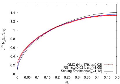
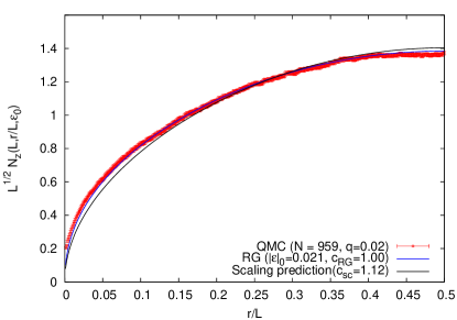
Figure 3: $L^{1/2}N_{z}(r)$ plotted versus $r/L$ in the power-law ordered Neel phase at $q=0.02$ (where $L=N+1$ for chains with $N=959$ and $N=479$ spins and open boundary conditions) and compared with the scaling prediction with a common best fit prefactor $c_{sc}$. Note that the deviation of the data from the scaling prediction cannot be simply ascribed to an overall multiplicative factor that grows with $N$, since the shape of the curves is slightly different. Data at both sizes is also fit to the best two-parameter fit corresponding to our RG improved perturbation theory result, and the agreement is seen to be excellent for the best fit values of $c_{RG}$ and $|\epsilon_{0}|$ listed in the legend.

This method has also been used in computations of ground state spin textures at ‘deconfined’ critical points in two dimensional $SU(2)$ and $SU(3)$ antiferromagnetsBanerjee_Damle_Alet1 ; Banerjee_Damle_Alet2 , as well as in very recent parallel work on developing a diagnostic for the presence of sharply-defined spinon excitationsYing_Sandvik in antiferromagnets.

We consider pure systems with periodic boundary conditions and total number of sites ranging from $N=60$ to $N=960$, as well as the corresponding open spin chains obtained by removing one site from the pure system. Our projection power is chosen to scale as $4N^{3}$ to ensure convergence to the ground state. We perform $\gtrsim 10^{5}$ equilibration steps followed by $\gtrsim 10^{6}$ Monte Carlo measurements to ensure that statistical errors are under control. In systems with a vacancy, we measure $\Phi(r)$ in the manner outlined above, and coarse-grain over pairs of successive sites to obtain our numerical results for the alternating part $N_{z}(r)$, which is to be thought of as living on bond-centers in this coarse-graining procedure. We have checked that our conclusions are not sensitive to the precise coarse-graining procedure used, although non-universal details, such as the overall amplitude of $N_{z}(r)$, do change.

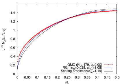
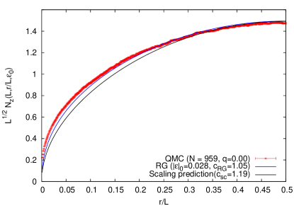
Figure 4: $L^{1/2}N_{z}(r)$ plotted versus $r/L$ in the power-law ordered Neel phase at $q=0.0$ (where $L=N+1$ for chains with $N=959$ and $N=479$ spins and open boundary conditions) and compared with the scaling prediction with a common best-fit prefactor $c_{sc}$. Note that the deviation of the data from the scaling prediction cannot be simply ascribed to an overall multiplicative factor that grows with $N$, since the shape of the curves is slightly different. Data at both sizes is also fit to the best two-parameter fit corresponding to our RG improved perturbation theory result, and the agreement is seen to be quite reasonable, but not perfect, for the best fit values of $c_{RG}$ and $|\epsilon_{0}|$ listed in the legend.

For the corresponding pure systems, we employ the singlet sector valence bond projection QMC techniqueSandvik_Evertz , and calculate the ground state spin-spin correlation function $C(j)=\langle\vec{S}(0)\cdot\vec{S}(j)\rangle$ for two sites separated by $j-1$ intervening sites ($j\leq N/2$, where $N$ is the total number of spins). To begin with, we scan the six-spin coupling $q=Q/4J$ and study the $q$ and $N$ dependence of $NC(N/2)$ as a convenient diagnostic that distinguishes the power-law Neel ordered phase at small $q$ from the spontaneously dimerized valence bond solid (VBS) ordered phase that is stabilized for large $q$. In the power-law Neel phase, $NC(N/2)$ grows (logarithmically) slowly with $N$, while in the VBS phase, it fall off rapidly with increasing $N$. Precisely at the critical point separating these two phases, we thus expect a crossing point for $NC(N/2)$ plotted against $q$ for various values of $N$. This is precisely what is seen in our data shown in Fig 1. From our data, we estimate that the critical point separating these two phases is located at $q_{c}\approx 0.04$ with an error of approximately $0.005$ estimated by extrapolating for the position of the crossing point (this estimate is consistent with the critical point found in Ref. Ying_Sandvik, ).

With this in hand, we compute the ground state spin texture in the corresponding chains with one site removed for several $q\leq q_{c}$ for a range of system sizes. The alternating part of the computed spin texture is then compared with the scaling predictions obtained by setting $\epsilon_{0}=0$, as well as with our RG improved perturbation theory predictions. The former represents a one-parameter fit of the data, with the overall amplitude $c$ being the only free parameter, while the latter should be thought of as a two parameter fit, with the bare value $\epsilon_{0}$ of the sine-Gordon coupling being the second fitting parameter.

In Fig (2), we first display our data for the alternating part of the spin texture and compare it with the scaling prediction at the putative critical point $q=q_{c}$ for two of our largest system sizes. As is clear from these two figures, the scaling prediction fits extremely well to all the data at both sizes. Furthermore, a two-parameter fit using the RG-improved perturbation theory result yields a best-fit value of $\epsilon_{0}$ indistinguishable from $\epsilon_{0}=0$. This confirms our identification of the critical point, since we expect that the bare coefficient of the marginally irrelevant cosine interaction is zero at this quantum phase transition.

This excellent fit to the scaling prediction should be contrasted with the results shown in Figs (3),(4), which show numerical results at two representative points in the power-law Neel phase compared with the one-parameter fit obtained from the scaling prediction. As is clear from these figures, the scaling prediction simply cannot provide a satisfactory account of the data for $q<q_{c}$, with the discrepancy being more pronounced for smaller $q$, that is, further away from the critical point. Furthermore, the observed deviations from scaling cannot be simply ascribed to an overall $N$ dependent prefactor that grows with system size, since the shapes of the curves are themselves slightly different from the scaling prediction.

In the same figures, we also show the best two-parameter fit obtained by using our RG improved perturbation theory result. Two points are worth noting regarding these two parameter fits: Firstly, the best-fit values of $|\epsilon_{0}|$ increase as one goes further away from $q=q_{c}$, consistent with the expectation that the bare coefficient of the cosine interaction vanishes as $q$ approaches $q_{c}$. Second, the RG improved perturbation theory provides a much better fit at $q=0.02$ than at the Heisenberg point $q=0$—again this is consistent with our expectations, since our calculation is perturbative in the renormalized coupling $\epsilon(L)$, and is therefore expected to provide a better approximation when the bare value of $|\epsilon_{0}|$ is smaller to begin with.

IV Discussion

We conclude by clarifying the relationship of our calculations with earlier calculations of the effect of vacancies on Sirker_Laflorencie ; Eggert_Affleck_impurities ; Brunel_Bocquet_Jolicoeur ; Fujimoto_Eggert on spin chains. These have typically focused on the low-field NMR Knight shift and relaxation rate $1/T_{1}$ in the presence of vacancies, or the impurity contribution to the zero-field spin structure factor and linear susceptibility of such chains. All these experimental observables are obtained from the knowledge of the zero field static and equal time spin correlations of the system at finite temperature, which has been the main focus of this body of work. In contrast, our results focus on local spin texture induced by the presence of vacancies at $T=0$, which is a quite different observable connected with the impurity contribution to the local susceptibility in the high-field regime in which the external field dominates over the thermal fluctuations.

V Acknowledgements

We acknowledge useful discussions with Ribhu Kaul, Nicolas Laflorencie, Gautam Mandal, Anders Sandvik, and Diptiman Sen, computational resources of the TIFR, and support from DST (India) grant DST-SR/S2/RJN-25/2006.

References

- (1) M. Takigawa, N. Motoyama, H. Eisaki, and S. Uchida, Phys. Rev. B 55, 14129 (1997).
- (2) D. A. Tennant et. al., Phys. Rev. B 71, 134412 (2005).
- (3) B. Lake, D. A. Tennant, C. D. Frost, S. E. Nagler, Nature Materials 4, 329 (2005).
- (4) B. Lake, D. A. Tennant, S. E. Nagler, Phys. Rev. B 71, 134412 (2005).
- (5) I. Affleck, Fields, Strings, and Critical Phenomena, Les Houches 1988, E. Brezin and J. Zinn-Justin (eds.), North-Holland, Amsterdam (1990).
- (6) R. R. P. Singh, M. E. Fisher, and R. Shankar, Phys. Rev. B 39, 2562 (1989).
- (7) I. Affleck, D. Gepner, H. Shultz, and T. Ziman, J Phys. A: Math. Gen. 22, 511 (1989).
- (8) V. Barzykin and I. Affleck, J Phys. A: Math. Gen. 32, 867 (1999).
- (9) E. Orignac, Eur. Phys. J. B 39, 335 (2004).
- (10) R. Chitra, S. Pati, H. R. Krishnamurthy, D. Sen, and S. Ramasesha, Phys. Rev. B 52, 6581 (1995).
- (11) S. Eggert, Phys. Rev. B 54, R9612 (1996).
- (12) R. Kenna, Nuclear Physics B 691 [FS], 292 (2004).
- (13) S. Sachdev, Phys. Rev. B 50, 13006 (1994).
- (14) A. W. Sandvik, Phys. Rev. Lett. 104, 177201 (2010).
- (15) A. Banerjee, K. Damle, and F. Alet Phys. Rev. B 82, 155139 (2010).
- (16) T. Senthil, L. Balents, S. Sachdev, A. Vishwanath, and M. P. A. Fisher, Phys. Rev. B 70, 144407 (2004).
- (17) A. W. Sandvik, Phys. Rev. Lett. 98, 227202 (2007).
- (18) R. K. Kaul, arXiv:1010.1937, unpublished.
- (19) A. W. Sandvik, V. N. Kotov, and O. P. Sushkov, Phys. Rev. Lett. 106, 207203 (2011).
- (20) A. Banerjee, K. Damle, and F. Alet, Phys. Rev. B 83, 235111 (2011).
- (21) J. Lou, A. W. Sandvik, N. Kawashima, Phys. Rev. B 80, 180414(R) (2009).
- (22) A. W. Sandvik, and H. G. Evertz, Phys. Rev. B 82, 024407 (2010).
- (23) A. Banerjee and K. Damle, J. Stat. Mech. (2010) P08017.
- (24) J. V. Jos , L. P. Kadanoff, S. Kirkpatrick, and D. R. Nelson, Phys. Rev. B 16, 1217 (1977).
- (25) T. Hirahara and A. Furusaki, Phys. Rev. B 63, 134438 (2001).
- (26) S. Eggert and I. Affleck, Phys. Rev. B 46, 10866 (1992).
- (27) Y. Tang and A. W. Sandvik, unpublished.
- (28) J. Sirker and N. Laflorencie, Europhys. Lett. 86, 57004 (2009).
- (29) S. Eggert and I. Affleck, Phys. Rev. Lett. 75, 934 (1995).
- (30) V. Brunel, M. Bocquet, and Th. Jolicoeur, Phys. Rev. Lett. 83, 2821 (1999).
- (31) S. Fujimoto and S. Eggert, Phys. Rev. Lett. 92, 037206 (2004).