Controller Synthesis for Robust Invariance of Polynomial Dynamical Systems using Linear Programming

Abstract.

In this paper, we consider a control synthesis problem for a class of polynomial dynamical systems subject to bounded disturbances and with input constraints. More precisely, we aim at synthesizing at the same time a controller and an invariant set for the controlled system under all admissible disturbances. We propose a computational method to solve this problem. Given a candidate polyhedral invariant, we show that controller synthesis can be formulated as an optimization problem involving polynomial cost functions over bounded polytopes for which effective linear programming relaxations can be obtained. Then, we propose an iterative approach to compute the controller and the polyhedral invariant at once. Each iteration of the approach mainly consists in solving two linear programs (one for the controller and one for the invariant) and is thus computationally tractable. Finally, we show with several examples the usefulness of our method in applications.

1. Introduction

The design of nonlinear systems remains a challenging problem in control science. In the past decade, building on spectacular breakthroughs in optimization over polynomial functions [Las01, Par03], several computational methods have been developed for synthesizing controllers for polynomial dynamical systems [PPR04, LHPT08]. These approaches have shown successful for several synthesis problems such as stabilization or optimal control in which Lyapunov functions and cost functions can be represented or approximated by polynomials. However, these approaches are not suitable for some other problems such as those involving polynomial dynamical systems with constraints on states and inputs, and subject to bounded disturbances.

In this paper, we consider a control synthesis problem for this class of systems. More precisely, given a polynomial dynamical system with input constraints and bounded disturbances, given a set of initial states $\underline{P}$ and a set of safe states $\overline{P}$, we aim at synthesizing a controller satisfying the input constraints and such that trajectories starting in $\underline{P}$ remain in $\overline{P}$ for all possible disturbances. This problem can be solved by computing jointly the controller and an invariant set for the controlled system which contains $\underline{P}$ and is included in $\overline{P}$ (see e.g. [Bla99]). We propose a computational method to solve this problem. We use parameterized template expressions for the controller and the invariant. Given a candidate polyhedral invariant, we show that controller synthesis can be formulated as an optimization problem involving polynomial objective functions over bounded polytopes. Recently, using various tools such as the blossoming principle [Ram89] for polynomials, multi-affine functions [BH06] and Lagrangian duality, it has been shown how effective linear programming relaxations can be obtained for such optimization problems [BG10]. We then propose an iterative approach to compute jointly a controller and a polyhedral invariant. Each iteration of the approach mainly consists in solving two linear programs and is thus computationally tractable. Finally, we show applications of our approach to several examples.

2. Problem Formulation

In this work, we consider a nonlinear affine control system subject to input constraints and bounded disturbances:

(2.1) $$\dot{x}(t)=f(x(t),d(t))+g(x(t),d(t))u(t),\;d(t)\in D\;,u(t)\in U$$

where $x(t)\in R_{X}\subseteq\mathbb{R}^{n}$ denotes the state of the system, $d(t)\in D\subseteq\mathbb{R}^{m}$ is an external disturbance and $u(t)\in U\subseteq\mathbb{R}^{p}$ is the control input. We assume that the vector field $f:\mathbb{R}^{n}\times\mathbb{R}^{m}\rightarrow\mathbb{R}^{n}$ and the control matrix $g:\mathbb{R}^{n}\times\mathbb{R}^{m}\rightarrow\mathbb{R}^{(n\times p)}$, defining the dynamics of the system, are multivariate polynomial maps. We also assume that the set of states is a bounded rectangular domain: $R_{X}=[\underline{x_{1}},\overline{x_{1}}]\times\dots\times[\underline{x_{n}},\overline{x_{n}}]$ with $\underline{x_{k}}<\overline{x_{k}}$ for all $k\in\{1,\dots,n\}$; and that the set of disturbances $D$ and the set of inputs $U$ are convex compact polytopes:

$$D=\left\{d\in\mathbb{R}^{m}|\;\alpha_{D,k}\cdot d\leq\beta_{D,k},\;\forall k\in\mathcal{K}_{D}\right\}\text{ and }U=\left\{u\in\mathbb{R}^{p}|\;\alpha_{U,k}\cdot u\leq\beta_{U,k},\;\forall k\in\mathcal{K}_{U}\right\}$$

where $\alpha_{D,k}\in\mathbb{R}^{m}$, $\beta_{D,k}\in\mathbb{R}$, $\alpha_{U,k}\in\mathbb{R}^{p}$, $\beta_{U,k}\in\mathbb{R}$, $\mathcal{K}_{D}$ and $\mathcal{K}_{U}$ are finite sets of indices. We will denote by $R_{D}=[\underline{d_{1}},\overline{d_{1}}]\times\dots\times[\underline{d_{m}},\overline{d_{m}}]$ the interval hull of polytope $D$, that is the smallest rectangular domain containing $D$; and by $V_{X}=\{\underline{x_{1}},\overline{x_{1}}\}\times\dots\times\{\underline{x_{n}},\overline{x_{n}}\}$ and $V_{D}=\{\underline{d_{1}},\overline{d_{1}}\}\times\dots\times\{\underline{d_{m}},\overline{d_{m}}\}$ the set of vertices of $R_{X}$ and $R_{D}$. The present work deals with controller synthesis for a notion of invariance defined as follows:

Definition 2.1.

Consider a set of states $P\subseteq R_{X}$ and a controller $h:R_{X}\rightarrow U$, the controlled system

(2.2) $$\dot{x}(t)=f(x(t),d(t))+g(x(t),d(t))h(x(t)),\;d(t)\in D,$$

is said to be $P$-invariant if all trajectories with $x(0)\in P$ satisfy $x(t)\in P$ for all $t\geq 0$.

Let us remark that this is a notion of robust invariance since it has to hold for all possible disturbances. Let $\underline{P}\subseteq\overline{P}\subseteq R_{X}$ be convex compact polytopes. In this paper, we consider the problem of synthesizing a controller $h$ for system (2.1) such that all controlled trajectories starting in $\underline{P}$ remain in $\overline{P}$ forever. This can be seen as a safety property where $\underline{P}$ is the set of initial states and $\overline{P}$ is the set of safe states. The problem can be solved synthesizing jointly a controller and a polyhedral invariant $P\subseteq R_{X}$ containing $\underline{P}$ and included in $\overline{P}$:

Problem 2.2.

Synthesize a controller $h:R_{X}\rightarrow U$ and a convex compact polytope $P$ such that $\underline{P}\subseteq P\subseteq\overline{P}$ and the controlled system (2.2) is $P$-invariant.

In the following, we describe an approach to solve this problem. To restrict the search space, we shall use parameterized template expressions for the controller $h$ and the invariant $P$. Firstly, we will impose the orientation of the facets of polytope $P$ by choosing normal vectors in the set $\{\gamma_{k}\in\mathbb{R}^{n}|\;k\in\mathcal{K}_{X}\}$ where $\mathcal{K}_{X}$ is a finite set of indices. Then, polytope $P$ can be written under the form

$$P=\left\{x\in\mathbb{R}^{n}|\;\gamma_{k}\cdot x\leq\eta_{k},\;\forall k\in\mathcal{K}_{X}\right\}$$

where the vector $\eta\in\mathbb{R}^{|\mathcal{K}_{X}|}$, to be determined, specifies the position of the facets. The facets of $P$ are denoted by $F_{k}$ for $k\in\mathcal{K}_{X}$, where $F_{k}=\left\{x\in\mathbb{R}^{n}|\;\gamma_{k}\cdot x=\eta_{k}\text{ and }\gamma_{i}\cdot x\leq\eta_{i},\;\forall i\in\mathcal{K}_{X}\setminus\{k\}\right\}.$ For simplicity, we will assume that the polytopes $\underline{P}$ and $\overline{P}$ are of the form: $\underline{P}=\{x\in\mathbb{R}^{n}|\;\gamma_{k}\cdot x\leq\underline{\eta}_{k},\;\forall k\in\mathcal{K}_{X}\}\text{ and }\overline{P}=\{x\in\mathbb{R}^{n}|\;\gamma_{k}\cdot x\leq\overline{\eta}_{k},\;\forall k\in\mathcal{K}_{X}\}.$ Then, the condition $\underline{P}\subseteq P\subseteq\overline{P}$ translates to $\underline{\eta}_{k}\leq\eta_{k}\leq\overline{\eta}_{k}$, for $k\in\mathcal{K}_{X}$. Secondly, we will search the controller $h$ in a subspace spanned by a polynomial matrix:

$$h(x)=H(x)\theta$$

where $\theta\in\mathbb{R}^{q}$ is a parameter to be determined and the matrix $H:\mathbb{R}^{n}\rightarrow\mathbb{R}^{(p\times q)}$ is a given multivariate polynomial map. The use of a template expression is natural when searching for a controller with a particular structure. The input constraint (i.e. for all $x\in R_{X}$, $h(x)\in U$) is then equivalent to

(2.3) $$\forall k\in\mathcal{K}_{U},\;\forall x\in R_{X},\;\alpha_{U,k}\cdot H(x)\theta\leq\beta_{U,k}.$$

Under these assumptions, the dynamics of the controlled system (2.2) can be rewritten under the form

$$\dot{x}(t)=f(x(t),d(t))+G(x(t),d(t))\theta,\;d(t)\in D,$$

where the matrix of polynomials $G(x,d)=g(x,d)H(x)$. From the standard characterization of invariant sets (see [Aub91]), it follows that the controlled system (2.2) is $P$-invariant if and only if

(2.4) $$\forall k\in\mathcal{K}_{X},\;\forall x\in F_{k},\forall d\in D,\;\gamma_{k}\cdot(f(x,d)+G(x,d)\theta)\leq 0.$$

Then, Problem 2.2 can be solved by computing vectors $\theta\in\mathbb{R}^{q}$ and $\eta\in\mathbb{R}^{|\mathcal{K}_{X}|}$ with $\underline{\eta}_{k}\leq\eta_{k}\leq\overline{\eta}_{k}$ for all $k\in\mathcal{K}_{X}$, and such that (2.3) and (2.4) hold. In the following, we first show how, given the vector $\eta\in\mathbb{R}^{|\mathcal{K}_{X}|}$ (and hence the polytope $P$), we can compute, using linear programming, the parameter $\theta$ (and hence the controller $h$) such that the controlled system (2.2) is $P$-invariant. Then, we show how to compute jointly the controller $h$ and the polytope $P$ using an iterative approach based on sensitivity analysis of linear programs. Before that, we shall review some recent results on linear relaxations for optimization of polynomials over bounded polytopes [BG10].

3. Optimization of Polynomials over Polytopes

In this section, we review some recent results of [BG10] that will be useful for solving Problem 2.2. Let us consider the following optimization problem involving a polynomial on a bounded polytope:

(3.1) $$\begin{array}[]{llr}\text{minimize}&c\cdot p(y)\\ \text{over}&y\in R,\\ \text{subject to}&a_{i}\cdot y\leq b_{i},&i\in I,\\ &a_{j}\cdot y=b_{j},&j\in J,\end{array}$$

where $p:\mathbb{R}^{m}\rightarrow\mathbb{R}^{n}$ is a multivariate polynomial map, $c\in\mathbb{R}^{n}$, $R=[\underline{y_{1}},\overline{y_{1}}]\times\dots\times[\underline{y_{m}},\overline{y_{m}}]$ is a rectangle of $\mathbb{R}^{m}$; $I$ and $J$ are finite sets of indices; $a_{k}\in\mathbb{R}^{m}$, $b_{k}\in\mathbb{R}$, for all $k\in I\cup J$. Let us remark that even though the polytope defined by the constraints indexed by $I$ and $J$ is unbounded in $\mathbb{R}^{m}$, the fact that we consider $y\in R$ which is a bounded rectangle of $\mathbb{R}^{m}$ results in an optimization problem on a bounded (not necessarily full dimensional) polytope of $\mathbb{R}^{m}$. Let $p^{*}$ denote the optimal value of problem (3.1). The approach presented in [BG10] allows us to compute a guaranteed lower bound $d^{*}$ of $p^{*}$. The approach is as follows. First, using the so-called blossoming principle [Ram89], we transform problem (3.1) into an equivalent optimization problem involving a multi-affine function on a polytope. The dual of this problem is then a linear program easily solvable and whose optimal value is a guaranteed lower bound of $p^{*}$.

3.1. Blossoming principle

Multi-affine functions form a particular class of multivariate polynomials. Essentially, a multi-affine function is a function which is affine in each of its variables when the other variables are regarded as constant.

Definition 3.1.

A multi-affine function $q:\mathbb{R}^{M}\rightarrow\mathbb{R}$ is a multivariate polynomial in the variables $z_{1},\dots,z_{M}$ where the degree of $g$ in each of its variables is at most $1$:

$$q(z)=q(z_{1},\dots,z_{M})=\sum_{(d_{1},\dots,d_{M})\in\{0,1\}^{M}}q_{(d_{1},\dots,d_{M})}z_{1}^{d_{1}}\dots z_{M}^{d_{M}}$$

where $q_{(d_{1},\dots,d_{M})}\in\mathbb{R}$ for all $(d_{1},\dots,d_{M})\in\{0,1\}^{M}$. A map $q:\mathbb{R}^{M}\rightarrow\mathbb{R}^{n}$ is a multi-affine map if each of its components is a multi-affine function.

It is shown in [BH06] that a multi-affine function $q$ is uniquely determined by its values at the vertices of a rectangle $R^{\prime}$ of $\mathbb{R}^{M}$. Moreover, for all $x\in R^{\prime}$, $q(x)$ is a convex combination of the values at the vertices so that we have the following result:

Lemma 3.2.

Let $q:\mathbb{R}^{M}\rightarrow\mathbb{R}$ be a multi-affine function and $R^{\prime}$ a rectangle of $\mathbb{R}^{M}$ with set of vertices $V^{\prime}$, then $\displaystyle{\min_{x\in R^{\prime}}q(x)=\min_{v\in V^{\prime}}q(v).}$

The blossoming principle (see e.g. [Ram89]) consists in mapping the set of polynomial maps to the set of multi-affine maps as follows. Let $p:\mathbb{R}^{m}\rightarrow\mathbb{R}^{n}$ be a polynomial map. Let $\delta_{1},\dots,\delta_{m}$ denote the degree of $p$ in the variables $y_{1},\dots,y_{m}$ respectively. Let $\Delta=\{0,\dots,\delta_{1}\}\times\dots\times\{0,\dots,\delta_{m}\}$, then for all $y\in\mathbb{R}^{m}$, $p(y)=(p_{1}(y),\dots,p_{n}(y))$, where for all $j=1,\dots,n$, the components $p_{j}:\mathbb{R}^{m}\rightarrow\mathbb{R}$ are multivariable polynomial functions that can be written under the form:

$$p_{j}(y)=p_{j}(y_{1},\dots,y_{m})=\sum_{(d_{1},\dots,d_{m})\in\Delta}p_{j,(d_{1},\dots,d_{m})}y_{1}^{d_{1}}\dots y_{m}^{d_{m}}$$

where $p_{j,(d_{1},\dots,d_{m})}\in\mathbb{R}$, for all $(d_{1},\dots,d_{m})\in\Delta$ and $j=1,\dots,n$.

Definition 3.3.

The blossom of the polynomial map $p:\mathbb{R}^{m}\rightarrow\mathbb{R}^{n}$ is the map $q:\mathbb{R}^{\delta_{1}+\dots+\delta_{m}}\rightarrow\mathbb{R}^{n}$ whose components are given for $j=1,\dots,n$ and $z=(z_{1,1},\dots,z_{1,\delta_{1}},\dots,z_{m,1},\dots,z_{m,\delta_{m}})\in\mathbb{R}^{\delta_{1}+\dots+\delta_{m}}$ by

$$q_{j}(z)=\sum_{(d_{1},\dots,d_{m})\in\Delta}p_{j,(d_{1},\dots,d_{m})}B_{d_{1},\delta_{1}}(z_{1,1},\dots,z_{1,\delta_{1}})\dots B_{d_{m},\delta_{m}}(z_{m,1},\dots,z_{m,\delta_{m}})$$

with

$$B_{d,\delta}(z_{1},\dots,z_{\delta})=\frac{1}{\left(\begin{smallmatrix}\delta\\ d\end{smallmatrix}\right)}\sum_{\sigma\in C(d,\delta)}z_{\sigma_{1}}\dots z_{\sigma_{d}}$$

where $C(d,\delta)$ denotes the set of combinations of $d$ elements in $\{1,\dots,\delta\}$.

Example 3.4.

The blossom of the polynomial map $p(x_{1},x_{2})=(x_{1}+x_{2}^{3},x_{1}^{2}x_{2}^{2})$ is $q:\mathbb{R}^{5}\rightarrow\mathbb{R}^{2}$ whose components are given by

$$\begin{array}[]{rll}q_{1}(z_{1,1},z_{1,2},z_{2,1},z_{2,2},z_{2,3})&=&\frac{1}{2}(z_{1,1}+z_{1,2})+z_{2,1}z_{2,2}z_{2,3}\\ q_{2}(z_{1,1},z_{1,2},z_{2,1},z_{2,2},z_{2,3})&=&z_{1,1}z_{1,2}\frac{1}{3}(z_{2,1}z_{2,2}+z_{2,2}z_{2,3}+z_{2,3}z_{2,1})\end{array}$$

From Definition 3.3, it follows that the blossom $q$ of the polynomial map $p$ satisfies the following properties [Ram89]:

1. It is a multi-affine map.

2. It satisfies the diagonal property: $q(z_{1},\dots,z_{1},\dots,z_{m},\dots,z_{m})=p(z_{1},\dots,z_{m}).$

3. Let $z,z^{\prime}\in\mathbb{R}^{\delta_{1}+\dots+\delta_{m}}$, with $z=(z_{1,1},\dots,z_{1,\delta_{1}},\dots,z_{m,1},\dots,z_{m,\delta_{m}})$ and $z^{\prime}=(z^{\prime}_{1,1},\dots,z^{\prime}_{1,\delta_{1}},$ $\dots,z^{\prime}_{m,1},\dots,z^{\prime}_{m,\delta_{m}}),$ we denote $z\cong z^{\prime}$ if, for all $j=1,\dots,m$, there exists a permutation $\pi_{j}$ such that $(z_{j,1},\dots,z_{j,\delta_{j}})=\pi_{j}(z^{\prime}_{j,1},\dots,z^{\prime}_{j,\delta_{j}})$. It is easy to see that $\cong$ is an equivalence relation. Moreover, for all $z\cong z^{\prime}$, $q(z)=q(z^{\prime})$.

The diagonal property clearly allows us to recast problem (3.1) for a multivariate polynomial map $p$ as a problem involving its blossom $q$ subject to inequality and equality constraints:

(3.2) $$\begin{array}[]{llr}\text{minimize }&c\cdot q(z)\\ \text{over }&z\in R^{\prime},\\ \text{subject to }&{a_{i}}^{\prime}\cdot z\leq b_{i},&i\in I\\ &a_{j}^{\prime}\cdot z=b_{j},&j\in J,\\ &z_{k,l}=z_{k,l+1},&\;k=1,\ldots,n,\;l=1,\ldots,\delta_{j}-1.\end{array}$$

where $R^{\prime}=[\underline{y_{1}},\overline{y_{1}}]^{\delta_{1}}\times\dots\times[\underline{y_{m}},\overline{y_{m}}]^{\delta_{m}}$ and the vectors $a_{k}^{\prime}$ are given for $k\in I\cup J$ by

$$a_{k}^{\prime}={(\frac{a_{k,1}}{\delta_{1}},\dots,\frac{a_{k,1}}{\delta_{1}},\dots,\frac{a_{k,m}}{\delta_{m}},\dots,\frac{a_{k,m}}{\delta_{m}})}.$$

3.2. Linear programming relaxation

In [BG10], based on Lemma 3.2, it is shown that the Lagrangian dual of problem (3.2) is actually a linear program. After some complexity reduction enabled by the properties of blossoms stated above, the following result can be stated:

Theorem 3.5 ([BG10]).

The dual of problem (3.2) is equivalent to the following linear program:

(3.3) $$\begin{array}[]{llr}\text{maximize}&t\\ \text{over}&t\in\mathbb{R},\;\lambda\in\mathbb{R}^{|I|},\;\mu\in\mathbb{R}^{|J|}\\ \text{subject to}&\lambda_{i}\geq 0,&i\in I\\ &t\leq c\cdot q(\overline{v})+\displaystyle{\sum_{i\in I}\lambda_{i}(a_{i}^{\prime}\cdot\overline{v}-b_{i})}+\displaystyle{\sum_{j\in J}\mu_{j}(a_{j}^{\prime}\cdot\overline{v}-b_{j})},&\overline{v}\in\overline{V^{\prime}}.\end{array}$$

where $\overline{V^{\prime}}=V^{\prime}/\cong$ with $V^{\prime}=\{\underline{y_{1}},\overline{y_{1}}\}^{\delta_{1}}\times\dots\times\{\underline{y_{m}},\overline{y_{m}}\}^{\delta_{m}}$. Moreover the optimal value $d^{*}$ of this linear program is a guaranteed lower bound of the optimal value $p^{*}$ of problem (3.1).

The previous theorem provides a simple and efficient way to compute a guaranteed lower bound of the minimal value of a polynomial on a bounded polytope. In the following section, we will show how this can be used to solve our controller synthesis problem.

4. Controller Synthesis

In this section, given polytope $P=\left\{x\in\mathbb{R}^{n}|\;\gamma_{k}\cdot x\leq\eta_{k},\;\forall k\in\mathcal{K}_{X}\right\}$, we show how to design a controller $h:R_{X}\rightarrow U$ such that the system (2.2) is $P$-invariant. As explained before, we search the controller in a subspace spanned by a polynomial matrix: $h(x)=H(x)\theta$ where $\theta\in\mathbb{R}^{q}$. Let $F(x,d)=f(x,d)+G(x,d)\theta$, it is a polynomial of degree $\delta_{1},\dots,\delta_{n},\rho_{1},\dots,\rho_{m}$ in the variables $x_{1},\dots,x_{n},d_{1},\dots,d_{m}$. Its blossom is $F_{b}=f_{b}+G_{b}\theta$ where $f_{b}$ and $G_{b}$ are the blossoms of $f$ and $G$ regarded as polynomials of degree $\delta_{1},\dots,\delta_{n},\rho_{1},\dots,\rho_{m}$. Let $H_{b}$ be the blossom of the matrix $H$ regarded as a polynomial map of degree $\delta_{1},\dots,\delta_{n}$ in the variables $x_{1},\dots,x_{n}$. Let $R_{X}^{\prime}=[\underline{x_{1}},\overline{x_{1}}]^{\delta_{1}}\times\dots\times[\underline{x_{n}},\overline{x_{n}}]^{\delta_{n}}$, $V_{X}^{\prime}=\{\underline{x_{1}},\overline{x_{1}}\}^{\delta_{1}}\times\dots\times\{\underline{x_{n}},\overline{x_{n}}\}^{\delta_{n}}$, $V_{D}^{\prime}=\{\underline{d_{1}},\overline{d_{1}}\}^{\rho_{1}}\times\dots\times\{\underline{d_{m}},\overline{d_{m}}\}^{\rho_{m}}$, $\overline{V_{X}^{\prime}}={V_{X}^{\prime}}/\cong$ and $\overline{V_{D}^{\prime}}={V_{D}^{\prime}}/\cong$.

We first establish sufficient conditions such that $h(x)\in U$ for all $x\in R_{X}$:

Lemma 4.1.

If for all $l\in\mathcal{K_{U}}$, for all $\overline{v_{X}}\in\overline{V_{X}^{\prime}}$, $\alpha_{U,l}\cdot H_{b}(\overline{v_{X}})\theta\leq\beta_{U,l}$, then for all $x\in R_{X}$, $h(x)\in U$.

Proof.

If for all $l\in\mathcal{K_{U}}$, for all $\overline{v_{X}}\in\overline{V_{X}^{\prime}}$, $\alpha_{U,l}\cdot H_{b}(\overline{v_{X}})\theta\leq\beta_{U,l}$, then using the third property of the blossom we have for all $l\in\mathcal{K_{U}}$, for all ${v_{X}}\in{V_{X}^{\prime}}$, $\alpha_{U,l}\cdot H_{b}(v_{X})\theta\leq\beta_{U,l}$. Since $H_{b}$ is a multi-affine map, Lemma 3.2 implies that for all $l\in\mathcal{K_{U}}$, for all $z\in R_{X}^{\prime}$, $\alpha_{U,l}\cdot H_{b}(z)\theta\leq\beta_{U,l}$. Then, using the diagonal property of the blossom, we obtain for all $l\in\mathcal{K_{U}}$, for all $x\in R_{X}$, $\alpha_{U,l}\cdot H(x)\theta\leq\beta_{U,l}$ which is equivalent to say that for all $x\in R_{X}$, $h(x)\in U$. ∎

The previous result gives a finite set of linear constraints which must be satisfied by parameter $\theta$. We now establish conditions ensuring that the polytope $P$ is an invariant for system (2.2). Let $k\in\mathcal{K}_{X}$, we will say that facet $F_{k}$ of the polytope $P$ is blocked if for all $x\in F_{k}$, for all $d\in D$, $\gamma_{k}\cdot(f(x,d)+G(x,d)\theta)\leq 0$. It is clear that system (2.2) is $P$-invariant if and only if all facets are blocked.

Lemma 4.2.

Let $\theta\in\mathbb{R}^{q}$ and $k\in\mathcal{K}_{X}$, then the facet $F_{k}$ is blocked if and only if the optimal value $p_{k}^{*}(\theta)$ of the following optimization problem is non negative:

(4.1) $$\begin{array}[]{llr}\text{minimize}&-\gamma_{k}\cdot(f(x,d)+G(x,d)\theta)\\ \text{over}&x\in R_{X},d\in R_{D}\\ \text{subject to}&\alpha_{D,j}\cdot d\leq\beta_{D_{j}},&j\in\mathcal{K}_{D},\\ &\gamma_{i}\cdot x\leq\eta_{i},&i\in\mathcal{K}_{X}\setminus\{k\},\\ &\gamma_{k}\cdot x=\eta_{k}.\end{array}$$

A guaranteed lower bound $d_{k}^{*}(\theta)$ of $p_{k}^{*}(\theta)$ is given by the optimal value of the following linear program:

(4.2) $$\begin{array}[]{lll}\text{maximize}&t\\ \text{over}&t\in\mathbb{R},\;\lambda^{k}\in\mathbb{R}^{|\mathcal{K}_{X}|},\tilde{\lambda}^{k}\in\mathbb{R}^{|\mathcal{K}_{D}|},\\ \text{subject to}&\displaystyle{\lambda_{i}^{k}}\geq 0,&i\in\mathcal{K}_{X}\setminus\{k\},\\ &{\tilde{\lambda}^{k}}_{j}\geq 0,&j\in\mathcal{K}_{D},\\ &t\leq-\gamma_{k}\cdot(f_{b}(\overline{v_{X}},\overline{v_{D}})+G_{b}(\overline{v_{X}},\overline{v_{D}})\theta)\\ &\;\;\;\;\;+\displaystyle{\sum_{i=1}^{|\mathcal{K}_{X}|}\displaystyle{\lambda_{i}^{k}}({\gamma_{i}}^{\prime}\cdot\overline{v_{X}}-\eta_{i})}+\displaystyle{\sum_{j=1}^{|\mathcal{K}_{D}|}{\tilde{\lambda}^{k}}_{j}(\alpha_{D,j}^{\prime}\cdot\overline{v_{D}}-\beta_{D,j})},&\overline{v_{X}}\in\overline{{V_{X}}^{\prime}},\;\overline{v_{D}}\in\overline{{V_{D}}^{\prime}}.\end{array}$$

where for all $i\in\mathcal{K}_{X}$ and all $j\in\mathcal{K}_{D}$ vectors ${\gamma_{i}}^{\prime}$ and $\alpha_{D,j}^{\prime}$ are given by:

$${\gamma_{i}}^{\prime}={(\frac{\gamma_{i,1}}{\delta_{1}},\dots,\frac{\gamma_{i,1}}{\delta_{1}},\dots,\frac{\gamma_{i,n}}{\delta_{n}},\dots,\frac{\gamma_{i,n}}{\delta_{n}})},\;\alpha_{D,j}^{\prime}={(\frac{\alpha_{D,j,1}}{\rho_{1}},\dots,\frac{\alpha_{D,j,1}}{\rho_{1}},\dots,\frac{\alpha_{D,j,m}}{\rho_{m}},\dots,\frac{\alpha_{D,j,m}}{\rho_{m}})}.$$

Proof.

Remarking that $F_{k}=R_{X}\cap F_{k}$ and $D=R_{D}\cap D$, the first part of the Proposition is obvious.
For the second part, let us remark that from the definition of the equivalence relation $\cong$, we have $(V_{X}^{\prime}\times V_{D}^{\prime})/\cong$ that is the same as $\overline{{V_{X}}^{\prime}}\times\overline{{V_{D}}^{\prime}}$. Then, we have just to apply the approach described in Section 3 where $y=(x,d)$ and the multivariate polynomial $p(y)$ is equal to $f(x,d)+G(x,d)\theta$. ∎

Now we show how to choose $\theta\in\mathbb{R}^{q}$ such that the associated controller satisfy for all $x\in R_{X}$, $h(x)\in U$ and the controlled system (2.2) is $P$-invariant.

Proposition 4.3.

Let $d^{*}$ and $\left(t^{*},({\lambda^{k*}})_{k\in\mathcal{K}_{X}},({\tilde{\lambda}^{k*}})_{k\in\mathcal{K}_{D}},\theta^{*}\right)$ be the optimal value and an optimal solution of the following linear program:

(4.3) $$\begin{array}[]{lll}\text{maximize}&t\\ \text{over}&t\in\mathbb{R},\;{\lambda}^{k}\in\mathbb{R}^{|\mathcal{K}_{X}|},\tilde{\lambda}^{k}\in\mathbb{R}^{|\mathcal{K}_{D}|},{\theta}\in\mathbb{R}^{q},&k\in\mathcal{K_{X}}\\ \text{subject to}&\displaystyle{\lambda_{i}^{k}}\geq 0,&k\in\mathcal{K_{X}},\quad i\in\mathcal{K}_{X}\setminus\{k\},\\ &{\tilde{\lambda}^{k}}_{j}\geq 0,&k\in\mathcal{K_{X}},\quad j\in\mathcal{K}_{D},\\ &\alpha_{U,l}\cdot H_{b}(\overline{v_{X}})\theta\leq\beta_{U,l},&l\in\mathcal{K_{U}},\quad\overline{v_{X}}\in\overline{V_{X}^{\prime}},\\ &t\leq-\gamma_{k}\cdot(f_{b}(\overline{v_{X}},\overline{v_{D}})+G_{b}(\overline{v_{X}},\overline{v_{D}})\theta)\\ &\;\;\;\;\;+\displaystyle{\sum_{i=1}^{|\mathcal{K}_{X}|}\displaystyle{\lambda_{i}^{k}}({\gamma_{i}}^{\prime}\cdot\overline{v_{X}}-\eta_{i})}+\displaystyle{\sum_{j=1}^{|\mathcal{K}_{D}|}{\tilde{\lambda}^{k}}_{j}(\alpha_{D,j}^{\prime}\cdot\overline{v_{D}}-\beta_{D,j})},&k\in\mathcal{K_{X}},\overline{v_{X}}\in\overline{{V_{X}}^{\prime}},\;\overline{v_{D}}\in\overline{{V_{D}}^{\prime}}.\end{array}$$

Then, if $d^{*}$ is positive, the controller $h(x)=H(x)\theta^{*}$ satisfy for all $x\in R_{X}$, $h(x)\in U$ and the controlled system (2.2) is $P$-invariant.

Proof.

We first start by remarking that problem (4.3) is equivalent to the following optimization problem:

(4.4) $$\begin{array}[]{lll}\text{maximize}&t\\ \text{over}&t\in\mathbb{R},\;{\theta}\in\mathbb{R}^{q}\\ \text{subject to}&\alpha_{U,l}\cdot H_{b}(\overline{v_{X}})\theta\leq\beta_{U,l},&l\in\mathcal{K_{U}},\quad\overline{v_{X}}\in\overline{V_{X}^{\prime}},\\ &t\leq d_{k}^{*}(\theta),&k\in\mathcal{K_{X}}\end{array}$$

where $d_{k}^{*}(\theta)$ is the optimal value of linear program (4.2). Then, if $d^{*}\geq 0$, this means that for the optimal $\theta^{*}$, we have for all $k\in\mathcal{K}_{X}$, $d_{k}^{*}(\theta^{*})\geq 0$. Therefore, by Lemma 4.2, all facets of $P$ are blocked and thus the controlled system (2.2) is $P$-invariant. The constraints on $\theta$ also ensures, by Lemma 4.1, that for all $x\in R_{X}$, $h(x)\in U$. ∎

5. Joint Synthesis of the Controller and the Invariant

In this section, we present an iterative approach for synthesizing jointly the controller $h$ and the invariant polytope $P$ solving Problem 2.2. It is based on sensitivity analysis of linear programs. At each iteration, we use a guess for the invariant polytope $P$. Following the approach described in the previous section, we try to synthesize a controller $h$ that renders $P$ invariant. If $P$ cannot be made invariant by this approach, we use sensitivity analysis of linear program (4.3) to modify $P$ and obtain a new guess for the invariant polytope. The procedure is repeated until Problem 2.2 is solved.

5.1. Sensitivity analysis

Let $\eta,\mu\in\mathbb{R}^{|\mathcal{K}_{X}|}$, let polytopes $P=\left\{x\in\mathbb{R}^{n}|\;\gamma_{k}\cdot x\leq\eta_{k},\;\forall k\in\mathcal{K}_{X}\right\}$ and $P_{\mu}=\left\{x\in\mathbb{R}^{n}|\;\gamma_{k}\cdot x\leq\eta_{k}+\mu_{k},\;\forall k\in\mathcal{K}_{X}\right\}$; $P_{\mu}$ can be seen as a perturbation of polytope $P$. The main result on sensitivity analysis is given by the following proposition:

Proposition 5.1.

Let $d^{*}$ and $\left(t^{*},({\lambda^{k*}})_{k\in\mathcal{K}_{X}},({\tilde{\lambda}^{k*}})_{k\in\mathcal{K}_{D}},\theta^{*}\right)$ denote the optimal value and an optimal solution of linear program (4.3), let $d^{*}_{\mu}$ denote the optimal value of linear program (4.3) where $\eta$ has been replaced by $\eta+\mu$, then

$$d^{*}_{\mu}\geq\displaystyle{\min_{k\in\mathcal{K}_{X}}(d^{*}-{\lambda^{k*}}\cdot\mu}).$$

Proof.

For all $k\in\mathcal{K}_{X}$, for all $\overline{v_{X}}\in\overline{{V_{X}}^{\prime}}$ and $\overline{v_{D}}\in\overline{{V_{D}}^{\prime}}$, we have:

$$\begin{array}[]{ll}&-\gamma_{k}\cdot(f_{b}(\overline{v_{X}},\overline{v_{D}})+G_{b}(\overline{v_{X}},\overline{v_{D}})\theta)+\displaystyle{\sum_{i=1}^{|\mathcal{K}_{X}|}\displaystyle{\lambda_{i}^{k*}}({\gamma_{i}}^{\prime}\cdot\overline{v_{X}}-\eta_{i}-\mu_{i})}+\displaystyle{\sum_{j=1}^{|\mathcal{K}_{D}|}{\tilde{\lambda}^{k*}}_{j}(\alpha_{D,j}^{\prime}\cdot\overline{v_{D}}-\beta_{D,j})}\\ =&-\gamma_{k}\cdot(f_{b}(\overline{v_{X}},\overline{v_{D}})+G_{b}(\overline{v_{X}},\overline{v_{D}})\theta)+\displaystyle{\sum_{i=1}^{|\mathcal{K}_{X}|}\displaystyle{\lambda_{i}^{k*}}({\gamma_{i}}^{\prime}\cdot\overline{v_{X}}-\eta_{i})}+\displaystyle{\sum_{j=1}^{|\mathcal{K}_{D}|}{\tilde{\lambda}^{k*}}_{j}(\alpha_{D,j}^{\prime}\cdot\overline{v_{D}}-\beta_{D,j})}-{\lambda^{k*}}\cdot\mu\\ \geq&t^{*}-{\lambda^{k*}}\cdot\mu\geq\displaystyle{\min_{k^{\prime}\in\mathcal{K}_{X}}(t^{*}-{\lambda^{k^{\prime}*}}\cdot\mu}).\end{array}$$

This shows that $\left(\displaystyle{\min_{k\in\mathcal{K}_{X}}(t^{*}-{\lambda^{k*}}\cdot\mu}),(\lambda^{k*})_{k\in\mathcal{K}_{X}},({\tilde{\lambda}^{k*}})_{k\in\mathcal{K}_{D}},\theta^{*}\right)$ is a feasible solution for linear program (4.3) where $\eta$ has been replaced by $\eta+\mu$. It follows that $d^{*}_{\mu}\geq\displaystyle{\min_{k\in\mathcal{K}_{X}}(t^{*}-{\lambda^{k*}}\cdot\mu})$ which leads to the expected inequality since $d^{*}=t^{*}$. ∎

The previous result has the following implications. Let us assume that we are not able to synthesize a controller rendering polytope $P$ invariant by solving the linear program (4.3), this means that $d^{*}\leq 0$. Then, the previous result tells us how to obtain a modified polytope $P_{\mu}$ in order to get $d^{*}_{\mu}\geq 0$ (or at least to get an improved $d^{*}_{\mu}\geq d^{*}$). This suggests that we can solve Problem 2.2 using an iterative approach described in the following paragraph.

5.2. Iterative approach

Initially, let us assume that we have an initial guess for the polytope $P$; one can for instance use $\overline{P}$ but other choices are possible. We use an iterative approach to solve Problem 2.2; each iteration consists of two main steps.

5.2.1. First step: synthesize a controller

Given polytope $P=\left\{x\in\mathbb{R}^{n}|\;\gamma_{k}\cdot x\leq\eta_{k},\;\forall k\in\mathcal{K}_{X}\right\}$, we use Proposition 4.3 to synthesize a controller $h$. Let $d^{*}$ and $\left(t^{*},({\lambda^{k*}})_{k\in\mathcal{K}_{X}},({\tilde{\lambda}^{k*}})_{k\in\mathcal{K}_{D}},\theta^{*}\right)$ denote the optimal value and an optimal solution of linear program (4.3). If $d^{*}\geq 0$, then we found a controller rendering $P$ invariant for the controlled system (2.2) and Problem 2.2 is solved. If $d^{*}<0$, then we move to the second step.

5.2.2. Second step: modify the polytope

We now try to find $\mu\in\mathbb{R}^{|\mathcal{K}_{X}|}$ ensuring that polytope $P_{\mu}=\left\{x\in\mathbb{R}^{n}|\;\gamma_{k}\cdot x\leq\eta_{k}+\mu_{k},\;\forall k\in\mathcal{K}_{X}\right\}$ will be invariant for the controlled system (2.2). For that purpose, Proposition 5.1 tells us that it is sufficient that $d^{*}-\lambda^{k*}\cdot\mu\geq 0$, for all $k\in\mathcal{K}_{X}$. The requirement that $\underline{P}\subseteq P_{\mu}\subseteq\overline{P}$ can be translated to $\underline{\eta_{k}}-\eta_{k}\leq\mu_{k}\leq\overline{\eta}_{k}-\eta_{k}$ for all $k\in\mathcal{K}_{X}$. Also, since sensitivity analysis is pertinent mainly for small perturbations, we impose that for all $k\in\mathcal{K}_{X}$, $-\varepsilon\leq\mu_{k}\leq\varepsilon$ where $\varepsilon$ is a parameter that can be tuned. Then, finding a suitable $\mu$ can be done by solving the following linear program:

(5.1) $$\begin{array}[]{llr}\text{maximize}&t\\ \text{over}&t\in\mathbb{R},\;\mu\in\mathbb{R}^{|\mathcal{K}_{X}|},\\ \text{subject to}&t\leq d^{*}-{\lambda^{k*}}\cdot\mu,&k\in\mathcal{K}_{X},\\ &\min(-\varepsilon,\underline{\eta_{k}}-\eta_{k})\leq\mu_{k}\leq\max(-\varepsilon,\underline{\eta_{k}}-\eta_{k}),&k\in\mathcal{K}_{X}.\end{array}$$

Let $(t^{*},\mu^{*})$ be a solution of this linear program. If the optimal value $t^{*}$ of this problem is non-negative then it is sufficient to prove that the controller $h:R_{X}\rightarrow U$ synthesized in the first step and polytope $P_{\mu^{*}}$ solve Problem 2.2. Otherwise, if $t^{*}<0$, then we go back to the first step and start a new iteration with $P=P_{\mu^{*}}$.

Remark 5.2.

Let us remark that the polytope $P_{\mu^{*}}$ computed by solving (5.1) may have empty facets. In order to avoid such situations, it may be useful to replace $\mu^{*}$ by $\tilde{\mu}^{*}$ such that $P_{\tilde{\mu}^{*}}$ has no empty facet and $P_{\mu^{*}}=P_{\tilde{\mu}^{*}}$ (see Figure 1). This can be done by solving a set of linear programs.

Figure 1. The polytope $P_{\mu^{*}}$ may have empty facets (center polytope), we replace $\mu^{*}$ by $\tilde{\mu}^{*}$ such that $P_{\tilde{\mu}^{*}}$ has no empty facet and $P_{\mu^{*}}=P_{\tilde{\mu}^{*}}$ (right polytope).

Let us discuss briefly the computational complexity of our approach. Each iteration mainly consists in solving two linear programs. The linear program (4.3) has $1+q+|\mathcal{K}_{X}|(|\mathcal{K}_{X}|+|\mathcal{K}_{D}|)$ variables and $|\mathcal{K}_{X}|(|\mathcal{K}_{X}|+|\mathcal{K}_{D}|+|\overline{V_{X}^{\prime}}|+|\overline{V_{D}^{\prime}}|-1)+|\mathcal{K}_{U}||\overline{V_{X}^{\prime}}|$ inequality constraints. Let us remark that $|\overline{V_{X}^{\prime}}|=(\delta_{1}+1)\times\dots\times(\delta_{n}+1)$ and $|\overline{V_{D}^{\prime}}|=(\rho_{1}+1)\times\dots\times(\rho_{n}+1)$. Since the complexity of linear programming is polynomial in average in the number of variables and constraints. It follows that the first step of the iteration has polynomial cost in the number of constraints of polytopes $P$, $D$ and $U$ and in the degrees of the polynomials. The linear program (5.1) has $1+|\mathcal{K}_{X}|$ variables and $2|\mathcal{K}_{X}|$ inequality constraints. It follows that the second step of the iteration has polynomial cost in the number of constraints of polytope $P$.

6. Examples

Our approach was implemented in Matlab; in the following, we show its application to a set of examples.

6.1. Moore-Greitzer jet engine model

We tested our approach on the following polynomial system, corresponding to a Moore-Greitzer model of a jet engine [KKK95]:

(6.1) $$\left\{\begin{array}[]{rcll}\dot{x}_{1}&=&-x_{2}-\frac{3}{2}x_{1}^{2}-\frac{1}{2}x_{1}^{3}+d,\\ \dot{x}_{2}&=&u.\end{array}\right.$$

We first work in the rectangle $R_{X}=[-0.2,0.2]^{2}$ with disturbance $d\in D=R_{D}=[-0.02,0.02]$. We want to synthesize a linear controller i.e $h(x_{1},x_{2})=\theta_{1}x_{1}+\theta_{1}x_{2}$ such that $h(x)\in U=[-0.35,0.35]$, for all $x\in R_{X}$. Let $\underline{P}$ and $\overline{P}$ be polytopes with $m=24$ facets with uniformly distributed orientations and tangent to the circles of center $(0,0)$ and of radius $0.01$ and $0.2$, respectively. Using our approach, we found the controller $h(x_{1},x_{2})=0.8076x_{1}-0.9424x_{2}$ rendering the polytope $P$ shown on the left part of Figure 2 invariant. We make a second experiment, working in the rectangle $R_{X}=[-0.2,0.2]^{2}$ with disturbance $d\in D=R_{D}=[-0.025,0.025]$. We want to synthesize a polynomial control whose degrees are $3$ in $x_{1}$ and $1$ in $x_{2}$ (i.e. the same as the vector field). $\underline{P}$ and $\overline{P}$ are polytopes with $m=8$ facets with uniformly distributed orientations and tangent to the circles of center $(0,0)$ and of radius $0.01$ and $0.2$, respectively. Using our approach, we found a controller rendering the polytope $P$ shown on the right part of Figure 2 invariant. The previous experiments show that by looking for controller of higher degrees, we may be able to find simpler invariants for larger disturbances.

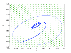
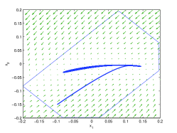
Figure 2. Left: Invariant polytope $P$ with $24$ facets and a trajectory of (6.1) illustrating the invariance for disturbance $d(t)=0.02\cos(0.5t)$. Right: Invariant polytope $P$ with $8$ facets and a trajectory of (6.1) illustrating the invariance for disturbance $d(t)=0.025\cos(0.1t)$.

6.2. Unicycle model

We now consider a simple model of a unicycle:

$$\left\{\begin{array}[]{rcll}\dot{x}&=&v\cos(\varphi),\\ \dot{y}&=&v\sin(\varphi),\\ \dot{\varphi}&=&\omega.\end{array}\right.$$

where $v$ and $\omega$ are the inputs of the system representing respectively the velocity and the angular velocity of the particle. In the following, we shall consider $v$ as a disturbance and $\omega$ as the control input. Using the change of coordinates $z_{1}=x\cos(\varphi)+y\sin(\varphi)$, and $z_{2}=x\sin(\varphi)-y\cos(\varphi)$, we obtain the following polynomial system.

(6.2) $$\left\{\begin{array}[]{rcll}\dot{z}_{1}&=&v-z_{2}\omega,\\ \dot{z}_{2}&=&z_{1}\omega.\end{array}\right.$$

We work in the rectangle $R_{X}=[-0.1,0.1]\times[0.9,1.1]$ with disturbance $v\in D=R_{D}=[0.96,1.04]$. We want to synthesize an affine controller $h(z_{1},z_{2})=\theta_{0}+\theta_{1}z_{1}+\theta_{2}z_{2}$. In this example, we do not impose constraints on the value of the input. $\underline{P}$ and $\overline{P}$ are defined as polytopes with $m=24$ facets with uniformly distributed orientations and tangent to the circles of center $(0,1)$ and radius $0.01$ and $0.1$ respectively. Using our approach, we found the controller $h(z_{1},z_{2})=1.0178+1.8721z_{1}-0.0253z_{2}$ rendering the polytope shown on Figure 3 invariant.

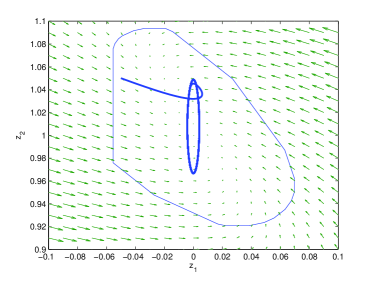
Figure 3. Invariant polytope $P$ with $24$ facets and a trajectory of (6.2) illustrating the invariance for disturbance $v(t)=1+0.04\cos(0.1t)$.

6.3. Rigid body motion

The last example is a model describing the motion of a rigid body. It is borrowed from [BI89]:

(6.3) $$\left\{\begin{array}[]{rcll}\dot{x}_{1}&=&u_{1},\\ \dot{x}_{2}&=&u_{2},\\ \dot{x}_{3}&=&x_{1}x_{2}.\end{array}\right.$$

We work in the rectangle $R_{X}=[-0.2,0.4]\times[-0.2,0.2]\times[-0.2,0.4]$. In this example, we do not consider disturbances. We want to synthesize a multi-affine controller i.e $h:\mathbb{R}^{3}\rightarrow\mathbb{R}^{2}$ (defined by sixteen parameters), such that $h(x)\in U=[-1,1]^{2}$, for all $x\in R_{X}$. Using our approach, we found a controller rendering the polytope with $18$ facets, shown on Figure 4, invariant.

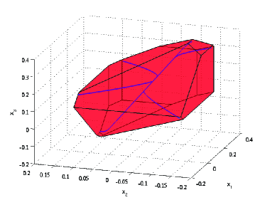
Figure 4. Invariant polytope $P$ with $18$ facets and trajectories of (6.3) illustrating the invariance.

7. Conclusion

In this paper, we have considered the problem of synthesizing controllers ensuring robust invariance of polynomial dynamical systems. Using the recent results of [BG10] on polynomial optimization over bounded polytopes, we have developed an iterative approach to solve this problem. It is mainly based on linear programming and therefore it is effective. We have shown applications to several examples which shows the usefulness of the approach. Future work will focus on a deeper theoretical analysis of the properties of the linear programming relaxations of polynomial optimization problems as well as their application to other classes of problems in control.

References

- [Aub91] J.P. Aubin. Viability Theory. Birkhauser, 1991.
- [BG10] M.A. Ben Sassi and A. Girard. Polytopic invariant verification and synthesis for polynomial dynamical systems via linear programming. 2010. Submitted, arXiv:1012.1256v1.
- [BH06] C. Belta and L.C.G.J.M. Habets. Controlling a class of nonlinear systems on rectangles. IEEE Transactions on Automatic Control, 51(11):1749–1759, 2006.
- [BI89] C.I. Byrnes and A. Isidori. New results and examples in nonlinear feedback stabilization. Systems & Control Letters, 12(4):437–442, 1989.
- [Bla99] F. Blanchini. Set invariance in control. Automatica, 35:1747–1777, 1999.
- [KKK95] M. Krstić, I. Kanellakopoulos, and P. Kokotović. Nonlinear and Adaptive Control Design. Wiley, 1995.
- [Las01] J.B. Lasserre. Global optimization with polynomials and the problem of moments. SIAM J. Optimization, 11(3):796–817, 2001.
- [LHPT08] J.B. Lasserre, D. Henrion, C. Prieur, and E. Tr lat. Nonlinear optimal control via occupation measures and lmi relaxations. SIAM J. Control Opt., 47(4):1643–1666, 2008.
- [Par03] P.A. Parrilo. Semidefinite programming relaxations for semialgebraic problems. Mathematical Programming Ser. B, 96(2):293–320, 2003.
- [PPR04] S. Prajna, P.A. Parrilo, and A. Rantzer. Nonlinear control synthesis by convex optimization. IEEE Trans. on Autom. Control, 49(2):1–5, 2004.
- [Ram89] L. Ramshaw. Blossoms are polar forms. Computer Aided Geometric Design, 6:323–358, 1989.