Elastic Scattering of ⁶He based on a Cluster Description

Abstract

Elastic scattering observables (differential cross section and analyzing power) are calculated for the reaction ⁶He(p,p)⁶He at projectile energies starting at 71 MeV/nucleon. The optical potential needed to describe the reaction is derived by describing ⁶He in terms of a ⁴He-core and two neutrons. The Watson first order multiple scattering ansatz is extended to accommodate the internal dynamics of a composite cluster model for the ⁶He nucleus scattering from a nucleon projectile. The calculations are compared with the recent experiments at the projectile energy of 71 MeV/nucleon. In addition, differential cross sections and analyzing powers are calculated at selected higher energies.

I Introduction

Traditionally, differential cross sections and spin observables played an important role in either determining the parameters in phenomenological optical models for proton-nucleus (p-A) scattering or in testing the accuracy and validity of microscopic models thereof. Specifically, elastic scattering of protons and neutrons from stable nuclei lead to a large body of work on optical potentials in which the two-nucleon interaction and the density matrix of the nucleus were taken as input to ab-initio calculations of first order optical potentials, either in a KMT or Watson expansion of the multiple scattering series, for which the primary goal was a deeper understanding of the reaction mechanism.

For exotic nuclei the theoretical emphasis is somewhat shifted. A goal of microscopic reaction theory is a construction of the scattering observables based on well-defined dynamical and structure quantities in order to, for example, examine structural sensitivities. Investigating the structure of halo nuclei, specifically ⁶He, has already inspired a large body of work including few-body models Zhukov:1993aw , Green’s Function Monte Carlo (GFMC) methods Pudliner:1997ck , and no-core shell model calculations Navratil:2004dp , so that ground state properties of ⁶He appear to be quite well understood.

Recently, elastic scattering of ⁶He off a polarized proton target has been measured for the first time at an energy of 71 MeV/nucleon Uesaka:2010mm ; Hatano:2005 . The experiment finds that the analyzing power becomes negative around 50^o which is not predicted by simple folding models for the optical potentials Weppner:2000fi ; Gupta:2000bu . The same calculations nevertheless describe the differential cross section at this energy reasonably well. This apparent “$A_{y}$ problem” conveys the inadequacy of using the same models which describe p-A scattering from stable nuclei for reactions involving halo nuclei. The obvious difference is the nuclear structure. While the typical stable nuclei for which folding models are very successful are mostly spherical, ⁶He can be understood in few-body models as a three-body system consisting of 2 neutrons ($n$) and a ⁴He core. Implementing this three-body structure in a cluster model, specifically in a reaction calculation for proton ($p$) scattering off ⁶He, was pioneered in Ref. Crespo:2006vg for calculating the reaction $p+^{6}$He at 717 MeV/nucleon, an energy at which the authors could employ the Born approximation. Based on the KMT formulation for the optical potential and more realistic wave functions for ⁶He, differential cross sections and analyzing powers were calculated in Ref. Crespo:2007zz at 297 MeV/per nucleon. For describing the differential cross section and the analyzing power at 71 MeV/nucleon, Ref. Uesaka:2010mm suggested a “cluster-folding” calculation having an explicit $\alpha$-core described by a phenomenological $p+^{4}$He optical potential.

In this work we want to extend the development of Ref. Crespo:2006vg by incorporating the cluster structure in an optical potential for the reaction $p+^{6}$He in such a way that the transition amplitude can be iterated to all orders (non-Born approximation). Our derivation of the optical potential is based on the Watson formulation for the multiple scattering theory, which not only allows to treat proton and neutron contributions to the structure separately Chinn:1993zza , but also lends itself naturally to taking into account the contributions of the $\alpha$-core and the two neutrons. The construction of an optical potential in which the separate contributions from the clusters are treated in a consistent fashion is achieved.

This article is organized as follows. In Section II we first present a short summary of the Watson optical potential for stable nuclei, and then extend this paradigm to the ⁶He nucleus consisting of an $\alpha$-core and two neutrons. In Section III we present our calculation for ⁶He$+p$ at 71 MeV/nucleon as well as at several higher energies and discuss their implications. Our conclusions are presented in Section IV. Three Appendices are devoted to the explicit derivation of the first order optical potential, the transformations between the different coordinate systems used in our calculations, and the calculation of the correlation densities between the clusters.

II The Folding Cluster Model

In order to derive a cluster ansatz for the target (projectile), and show how it can consistently be incorporated into a folding approach for the optical potential, we will for the convenience of the reader give a summary of the essential ingredients and underlying assumptions.

II.1 The Watson Optical Potential for Single Scattering

Let $H=H_{0}+V$ be the Hamiltonian for the nucleon-nucleus system (A+1 body system), where the interaction $V=\sum_{i}^{A}v_{0i}$ consists of all two-nucleon interactions $v_{0i}$ between the projectile (“$0$”) and a target nucleon (“$i$”). The free Hamiltonian is given by $H_{0}=h_{0}+H_{A}$, where $h_{0}$ describes the kinetic energy of the projectile, while the target Hamiltonian $H_{A}$ satisfies $H_{A}|\Psi_{A}\rangle=E_{A}|\Psi_{A}\rangle$, with $|\Psi_{A}\rangle$ being the ground state of the target.

The transition amplitude for the scattering of the projectile from the target is then given by a Lippmann-Schwinger equation, $T=V+VG_{0}T$, where the propagator $G_{0}$ is an (A+1) body operator given by

$$G_{0}(E)=(E-h_{0}-H_{A}+i\varepsilon)^{-1},$$ (1)

with $E$ being the total energy of the system. One way to tackle the many-body scattering problem is the spectator expansion Siciliano:1977zz , which writes the transition amplitude as $T=\sum_{i=1}^{A}T_{0i}$, so that

$$T_{0i}=v_{0i}+v_{0i}G_{0}(E)T.$$ (2)

This allows the sum of all interactions between projectile ‘$0$’ and nucleon ‘$i$’ by a formal reordering of the multiple scattering series according to Watson,

$$T_{0i}={\hat{\tau}}_{0i}+{\hat{\tau}}_{0i}G_{0}(E)\sum_{j\neq i}T_{0j},$$ (3)

where

$${\hat{\tau}}_{0i}=v_{0i}+v_{0i}G_{0}(E){\hat{\tau}}_{0i}.$$ (4)

The term ${\hat{\tau}}_{0i}$ of Eq. (4) only involves the interaction between pairs, namely particles ‘$0$’ and ‘$i$’, whereas the propagator $G_{0}(E)$ is still an (A+1)-body operator. The multiple scattering series of Eq. (3) can directly serve as starting point for constructing the transition amplitude for elastic scattering as shown in Refs. Crespo:2006vg ; Crespo:2007zz ; Crespo:2001nn .

When focusing on elastic scattering, the projection $P$ onto the ground state $|\Phi_{A}\rangle$ is introduced so that $[G_{0}(E),P]=0$. Here we define $P=\frac{|\Phi_{A}\rangle\langle\Phi_{A}|}{\langle\Phi_{A}|\Phi_{A}\rangle}$ and $P+Q={\bf 1}$, where $Q$ projects onto the orthogonal space. This allows the separation of the transition amplitude into two pieces,

$$T = U+UG_{0}(E)PT$$ (5)

$$U = V+VG_{0}(E)QU,$$ (6)

with $U$ being the optical potential operator. The transition operator for elastic scattering may then be defined as $T_{el}=PTP$, so that

$$T_{el}=PUP+PUPG_{0}(E)PT_{el}$$ (7)

is a one-body integral equation. Of course, it requires the knowledge of $PUP$, which has to contain the complete information about the many-body character of the problem. The formulations for the transition matrix for elastic scattering, given in Eqs. (3) and (6), are equivalent though truncations in the expansions are not.

The first order term of $U$ can be defined as

$$U=\sum_{i=1}^{A}U_{i}\approx\sum_{i=1}^{A}\tau_{0i},$$ (8)

with

$${\tau_{0i}}=v_{0i}+v_{0i}G_{0}(E)Q{\tau_{0i}}.$$ (9)

Because of the appearance of the projection operator $Q$ in Eq. (8), the quantity $\tau_{0i}$ can not yet be related to a two nucleon interaction. Defining a transition operator ${\hat{\tau}}_{0i}$, according to Eq. (4), allows the explicit relation to $\tau_{0i}$:

$${\hat{\tau}}_{0i} = v_{0i}+v_{0i}G_{0}(E)\left[P+Q\right]{\hat{\tau}}_{0i}$$ (10)

$$= \tau_{0i}+\tau_{0i}G_{0}(E)P{\hat{\tau}}_{0i},$$

so that one obtains the exact relations Chinn:1993zza

$$\tau_{0i}={\hat{\tau}}_{0i}-\tau_{0i}G_{0}(E)P{\hat{\tau}}_{0i}={\hat{\tau}}_{0i}-{\hat{\tau}_{0i}}G_{0}(E)P\tau_{0i}.$$ (11)

Taking into account the iso-spin character of the target nucleons instead of just summing over $A$ nucleons can be easily done by splitting Eq. (8) into two parts under the assumption that the projectile ‘0’ is a proton, Eq. (8) becomes:

$$U_{p}=\sum_{i=1}^{Z}\tau_{0i}^{pp}+\sum_{i=1}^{N}\tau_{0i}^{np}\equiv U_{p}^{Z}+U_{p}^{N},$$ (12)

where the integral Eq. (11) has to be solved separately for proton-proton (pp) and neutron-proton (np) interactions. This clearly indicates that the optical potential for the scattering of a proton ($U_{p}$) from a target nucleus differs from the optical potential for the scattering of a neutron ($U_{n}$) from the same target. Moreover, and more important for the present considerations, the folding with the proton and neutron density matrices is cleanly separated, which is not the case if one uses an optical potential in the formulation of Kerman-McManus-Thaler (KMT) KMT . A numerical study for $p+^{11}Li$ between a KMT formulation and Watson expansion of Eq. (3) has been carried out in Ref. Crespo:2001nn with the finding that truncations at the same order of the series though being similar at small momentum transfer show differences at the higher momentum transfers. This should not be surprising when considering the nonlinear relation of the free two-nucleon t-matrix, Eq. (11), to the quantity $\tau_{0i}$ entering the optical potential which is the driving term of the final scattering integral equation, Eq. (7). For the $n+d$ system, for which exact solutions of the Faddeev equations exist, optical potentials for elastic scattering were constructed in Kuros:1997zz indicating that first order approximations are only valid for smaller momentum transfers.

The propagator of Eq. (1) needs to be examined in more detail since it still is an (A+1)-body operator. Only if the target Hamiltonian $H_{A}$ is approximated by a c-number, $G_{0}(E)$ becomes a one-body operator and Eq. (4) can be identified with the free nucleon-nucleon (NN) t-matrix at an appropriate energy E. Reducing $H_{A}$ to a c-number is the standard impulse approximation (or extreme closure approximation) which has been widely used throughout the literature. The impulse approximation is believed to be a reasonable approximation in intermediate energy nuclear physics, i.e. in an energy regime where the kinetic energy of the projectile is large compared to excitation energies of the target, however the validity of this assumption has to be tested for individual cases under consideration.

II.2 First Order Folding Optical Potential

In this section we will give the explicit expressions for the ‘traditional’ first order Watson optical potential. Starting from those expressions will lead in a straightforward fashion to an optical potential where the nucleus is treated as a composite of clusters. Based on Eqs. (7) and (8) the first order optical potential as function of external momenta $\bf{k}$ and ${\bf{k}}^{\prime}$ is given by

$$\langle{\bf{k}}^{\prime}|\langle\phi_{A}|PUP|\phi_{A}\rangle{\bf{k}}\rangle\equiv U_{el}({\bf{k}}^{\prime},{\bf{k}})=\sum_{i=N,P}\left\langle{\bf{k}}^{\prime}|\langle\phi_{A}|\hat{\tau}_{0i}({\cal{E}})|\phi_{A}\rangle{\bf{k}}\right\rangle\equiv\langle{\hat{\tau}}_{0i}\rangle,$$ (13)

where ${\cal{E}}$ is the energy of the system. The summation over $i$ indicates that one has to sum over $N$ neutrons and $Z$ protons. The structure of Eq. (13) is graphically indicated by Fig. 1, ${\bf{k}}_{i}$ and ${\bf{k}}_{i}^{\prime}$ are internal variables of the struck target nucleon, ${\bf{p}}_{0}$ and ${\bf{p}}_{0}^{\prime}$ are external target variables. In the following derivation, we will sum over $A$ nucleons for clarity of presentation. However it should be emphasized that in practice a sum over $N$ neutrons and $Z$ protons, as indicated in Eq. (11), is done. The energy of the $\hat{\tau}_{0i}$ operator, $\cal{E}$, is a dynamical variable which depends on the total energy of the system and the energy of the spectator Elster:1997as similarly to a three-body problem. In this work the common approximation to fix it at half the laboratory energy will be used.

We consider a frame of reference in which ${\bf k_{0}}$ is the momentum of the projectile, and ${\bf p_{0}}$ is the momentum of the target. The individual nucleons inside the target have momenta $({\bf{k}}_{1},{\bf{k}}_{2},...{\bf{k}}_{A})$. Thus

$$\langle{\bf{k}}_{1}{\bf{k}}_{2}{\bf{k}}_{3}{\bf{k}}_{4}...{\bf{k}}_{A}|\phi_{A}\rangle=\delta({\bf{k}}_{1}+{\bf{k}}_{2}+{\bf{k}}_{3}+{\bf{k}}_{4}...+{\bf{k}}_{A}-{\bf{p}}_{0})\langle{\bf\zeta_{1}\zeta_{2}\zeta_{3}\zeta_{4}...\zeta_{A-1}}|\phi_{A}\rangle,$$ (14)

where the delta function determines the conservation of the absolute momentum for the center of mass (c.m.) frame of the nucleus, and ${\bf{\zeta}}_{i}$ represent the relative momenta of the individual nucleons in the target. The reason for using relative momenta is that the wave functions are naturally expressed in such a basis to manifestly express Galilean invariance, so any input into the theory will be in terms of the internal momenta ${\bf\zeta_{i}}$ and not ${\bf{k}}$. In first order, which is the concern of this work, we only need the momentum of the struck nucleon, namely ${\bf{k}}_{1}={\bf\zeta_{1}}+\frac{{\bf{p}}}{A}$. Changing integration variables from absolute to relative momenta, only the single particle density matrices, $\rho({\bf\zeta_{1}^{\prime},\zeta_{1}})$, are employed. They are used to describe the dependence of one particle’s relative motion to the remaining (A-1)-core,

$$\rho({\bf\zeta_{1}^{\prime},\zeta_{1}})\equiv\int\prod_{l=2}^{A-1}d{\bf\zeta_{l}^{\prime}}\int\prod_{j=2}^{A-1}d{\bf\zeta_{j}}\langle\phi_{A}|{\bf{\zeta}}_{1}^{\prime}{\bf{\zeta}}_{2}^{\prime}{\bf{\zeta}}_{3}^{\prime}{\bf{\zeta}}_{4}^{\prime}...{\bf{\zeta}}_{A-1}^{\prime}\rangle\;\langle{\bf{\zeta}}_{1}{\bf{\zeta}}_{2}{\bf{\zeta}}_{3}{\bf{\zeta}}_{4}...{\bf{\zeta}}_{A-1}|\phi_{A}\rangle.$$ (15)

The NN $\hat{\tau}_{01}$-matrix can always be written in relative coordinates as

$$\langle{\bf{q}}_{0}^{\prime}{\bf{q}}_{1}^{\prime}|\hat{\tau}_{01}({\cal E})|{\bf{q}}_{0}{\bf{q}}_{1}\rangle=\delta({\bf{q}}_{0}^{\prime}+{\bf{q}}_{1}^{\prime}-{\bf{q}}_{0}-{\bf{q}}_{1})\left\langle\frac{1}{2}({\bf{q}}_{0}^{\prime}-{\bf{q}}_{1}^{\prime})\big{|}\hat{\tau}_{01}({\cal E})\big{|}\frac{1}{2}({\bf{q}}_{0}-{\bf{q}}_{1})\right\rangle,$$ (16)

where the $\delta$-function indicates the momentum conservation of the two-nucleon pair. This leads to the following expression for the optical potential of Eq. (13),

$$\langle\hat{\tau}_{01}\rangle = \;\int d{\bf\zeta_{1}^{\prime}}\;\int d{\bf\zeta_{1}}\;\delta({\bf{k}}^{\prime}+{\bf{p}}_{0}^{\prime}-{\bf{k}}-{\bf{p}}_{0})\;$$ (17)

$$\left\langle\frac{1}{2}\left({\bf{k}}^{\prime}-{\bf\zeta_{1}^{\prime}}-\frac{{\bf{p}}_{0}^{\prime}}{A}\right)\Big{|}{\hat{\tau}}_{01}({\cal{E}})\Big{|}\frac{1}{2}\left({\bf{k}}-{\bf\zeta_{1}}-\frac{{\bf{p}}_{0}}{A}\right)\right\rangle\;\rho({\bf\zeta_{1}^{\prime}},{\bf\zeta_{1}})$$

$$\delta\left(\zeta_{1}^{\prime}-\zeta_{1}-\frac{A-1}{A}({\bf{k}}-{\bf{k}}^{\prime})\right),$$

which explicitly gives the following relation

$${\bf\zeta_{1}^{\prime}}-{\bf\zeta_{1}}=\frac{A-1}{A}({\bf{k}}-{\bf{k}}^{\prime}),$$ (18)

relating the relative variables ${\bf\zeta}$ directly to the external variables. For convenience, in the practical calculation, the definition

$${\bf{K}} \equiv \frac{1}{2}({\bf{k}}^{\prime}+{\bf{k}})$$

$${\bf{q}} \equiv {\bf{k}}^{\prime}-{\bf{k}}=\frac{A}{A-1}({\bf\zeta_{1}}-{\bf\zeta_{1}^{\prime}})$$

$${\bf{P}} \equiv \frac{1}{2}({\bf\zeta_{1}^{\prime}}+{\bf\zeta_{1}}),$$ (19)

where $\bf{q}$ is the momentum transfer and $\bf{K}$ is orthogonal to it, is used. After a series of variable transformations, which are outlined in Appendix A, one obtains for folding single-particle optical potential

$$U_{el}({\bf{q}},{\bf{K}})=$$ (21)

$$\sum_{i=n,p}\int d{\bf{P}}\hat{\tau}_{0i}\left({\bf{q}},\frac{1}{2}\left(\frac{A+1}{A}{\bf{K}}-{\bf{P}}\right),{\cal{E}}\right)\;\rho_{i}\left({\bf{P}}-\frac{A-1}{2A}{\bf{q}},{\bf{P}}+\frac{A-1}{2A}{\bf{q}}\right).$$

The above expression shows that one has to carry out a three-dimensional integration over the NN t-matrix and the nuclear density matrix. We are employing Monte Carlo methods for the actual computation.

II.3 Cluster Model for the Target Nucleus

Halo nuclei exhibit the distinctive feature of a usually tightly bound core and loosely bound valence nucleons. For exploring bound state properties a cluster model has been quite successful (see e.g.  Zhukov:1993aw ; Ghovanlou:1974zza ). Here we propose to employ a cluster model for the optical potential of ⁶He, and thus view ⁶He as a cluster of a tightly bound $\alpha$-particle and two valence neutrons. As explained in the previous sections, the first order folding optical potential uses the single nucleon density as a basic ingredient. That means, in the standard formulation of the optical potential, one deals with one active nucleon at a time, and then sums over all active nuclei. This paradigm can be naturally extended to a cluster model. The only additional consideration which needs to be taken into account is that now there is an intrinsic motion between the different pieces of the cluster. In order to accommodate this let us define a Jacobi momentum ${\bf p_{j}}$, representing the relative momentum of the active cluster and the spectator clusters, as

$${{\bf{p}}_{j}}_{i}=\frac{1}{A}({A_{s}}_{i}{\bf{p}}_{i}-A_{i}{\bf{p_{s}}}_{i}),$$ (22)

where the index $i$ characterizes a particular cluster and the index $s_{i}$ represents the spectators for the $i$th cluster. Since this is a Jacobi momentum it is invariant in all frames. The underlying belief is that there is a strongly peaked active cluster momentum, centered about ${\bf p_{i}}$, which is different from the other spectator cluster momentum, ${\bf p_{s}}_{i}$. If the nucleons are assumed to be largely independent of each other, as in a single particle picture, then ${{\bf{p}}_{j}}_{i}$ = 0, and the single-particle optical potential re-emerges.

With these additional momenta we can define a correlation density similar to the traditional density of Eq. (15):

$$\rho_{corr}({{\bf{p}}_{j}}_{1},{{\bf{p}}_{j}}^{\prime}_{1})\equiv\int\prod_{l=2}^{N_{c}}d{{{\bf{p}}_{j}}^{\prime}_{l}}\int\prod_{m=2}^{N_{c}}d{{{\bf{p}}_{j}}_{m}}\langle\phi_{A}|{\bf{p_{j}}}^{\prime}_{1}{\bf{p_{j}}}^{\prime}_{2}...{\bf{p_{j}}}^{\prime}_{N_{c}}\rangle\;\langle{\bf{p_{j}}}_{1}{\bf{p_{j}}}_{2}...{\bf{p_{j}}}_{N_{c}}|\phi_{A}\rangle,$$ (23)

where $N_{c}$ is the number of total clusters in the target. For the ⁶He system studied here $N_{c}=3$. The particular view in this model is that nucleons within a specific cluster move with the same c.m. momentum, which in turn is correlated with the momentum of the spectator clusters. This product of densities must conserve the overall momentum in the intrinsic frame of the nucleus. It further follows that the sum of all relative momenta in the cluster must be zero. In this work, we choose to work with the three-body cluster orbital shell model approximation (COSMA) density Zhukov:1994zz ; Zhukov:1991 .

In order to match the choice of momenta to those of the optical potential of the previous subsection, we define

$${{\bf{\cal P}}_{j}}_{i}=\frac{{{\bf{p}}_{j}}_{i}+{{\bf{p}}_{j}}^{\prime}_{i}}{2},$$ (24)

which is similar to the definitions of ${\bf{P}}$ and ${\bf{K}}$ defined in Eq. (19). Thus, the new cluster optical model provides an additional sum over the number of clusters

$$U_{el}({\bf{q}},{\bf{K}}) = \sum_{c=1,N_{c}}\;\sum_{i=n_{c},p_{c}}\int d{\bf{P}}\;d{{\bf{\cal P}}_{j}}_{c}\;\rho_{corr}({{\bf{\cal P}}_{j}}_{c})$$ (25)

$$\hat{\tau}_{0i}\left({\bf{q}},\frac{1}{2}\left(\frac{A+1}{A}{\bf{K}}-{\bf{P}}\right),{\cal{E}}\right)\;{{\rho}_{c}}_{i}\left({\bf{P}}-\frac{A-1}{2A}{\bf{q}},{\bf{P}}+\frac{A-1}{2A}{\bf{q}}\right),$$

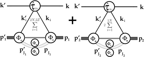
Figure 2: Diagram for the cluster optical potential for ⁶He based on the single-scattering approximation.

where each cluster now defines its own optical potential. With this, the optical potential for ⁶He consists of two pieces as indicated in Fig. 2, an optical potential for the $\alpha$-core and one for each of the two neutrons, both linked by the correlation density between the clusters,

$${}^{{}^{6}\rm{He}}U_{el}({\bf{q}},{\bf{K}})=U_{\alpha}+2U_{n}=$$ (27)

$$\sum_{i=N,P}\int d{\bf{P}}\;d{{\bf{\cal P}}_{j}}_{\alpha}\;\rho_{corr}({{\bf{\cal P}}_{j}}_{\alpha})\;\hat{\tau}_{0i}\left({\bf{q}},\frac{1}{2}\left(\frac{A+1}{A}{\bf{K}}-{\bf{P}}\right),{\cal{E}}\right)\;{{\rho}_{\alpha}}_{i}\left({\bf{P}}-\frac{A-1}{2A}{\bf{q}},{\bf{P}}+\frac{A-1}{2A}{\bf{q}}\right)$$

$$+2\int d{\bf{P}}\;d{{\bf{\cal P}}_{j}}_{n}\;\rho_{corr}({{\bf{\cal P}}_{j}}_{n})\;\hat{\tau}_{0i}\left({\bf{q}},\frac{1}{2}(\frac{A+1}{A}{\bf{K}}-{\bf{P}}),{\cal{E}}\right)\;{\rho}_{n}\left({\bf{P}}-\frac{A-1}{2A}{\bf{q}},{\bf{P}}+\frac{A-1}{2A}{\bf{q}}\right).$$

The cluster optical potential involves now a six-dimensional integration, which we again carry out with Monte Carlo methods. In addition, care must be taken to evaluate each cluster in the c.m. frame between projectile and cluster, since the scattering takes place in intrinsically different frames as dictated by the variable ${\bf{\cal P}}_{j}$. However, the final optical potential for the nucleus ⁶He must be evaluated in the c.m. frame of the target+projectile system. Thus, the initial step in the calculation involves first the evaluation of each cluster optical potential separately, and then boosting each to the target+projectile system. The explicit details of these transformations are given in Appendix B.

Furthermore, it is important to note that each cluster optical potential contains the correlation density. Through its variable ${\bf{\cal P}}_{j}$ the momenta of the active particles are constrained. An explicit derivation of the correlation density for the ⁶He nucleus is given in Appendix C.

III Results and Discussion

In this section we evaluate the differential cross section and the analyzing power for elastic scattering of ⁴He and ⁶He using non-local optical potentials in first order in the Watson multiple scattering expansion. Specifically, we want to test the influence of the cluster formulation presented in Section II.C on those observables compared to single-particle optical potentials of the same order in the multiple scattering expansion. We start with considering the recent experimental data for ⁶He at 71 MeV/nucleon Uesaka:2010mm , then we continue our investigation at slightly higher energies in order to gain some insight on the behavior of the elastic scattering observables as function of projectile energy.

As a nucleon-nucleon (NN) interaction we use the nonlocal Nijm-I potential of the Nijmegen group Stoks:1993tb , which describes the NN data below 350 MeV laboratory energy with a $\chi^{2}\approx 1$. For the density matrix of ⁶He the COSMA density of Refs. Zhukov:1994zz ; Zhukov:1991 is used. This density consists of harmonic oscillator wave functions for the s- and p-shell. The parameters are fitted such that ⁶He has a charge radius of 1.77 fm and a matter radius of 2.57 fm.

In addition the elastic scattering observables for proton scattering off ⁴He is calculated. The proton and neutron density matrix for ⁴He is obtained from a microscopic Hartree-Fock-Bogoliubov (HFB) calculation of Ref. HFB , which uses the Gogny D1S finite range effective interaction Gogny . The HFB calculation produces a mean-field potential, which in turn is used to modify the free NN interaction inside the nucleus Chinn:1995qn ; Chinn:1993zz . This modification of the free NN t-matrix has proved to be important in the description of closed shell nuclei at projectile energies below 150 MeV.

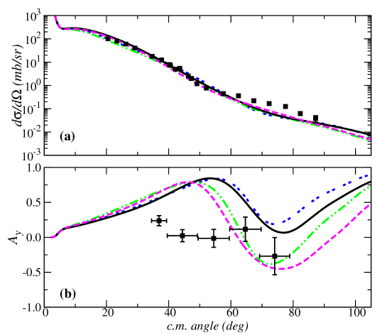
Figure 3: (color online) The angular distribution of the differential cross section,$\frac{d\sigma}{d\Omega}$, (upper panel (a)) and the analyzing power, $A_{y}$, (lower panel (b)) for elastic scattering ⁶He at projectile energy 71 MeV/nucleon as function of the c.m. angle. The calculations are performed with optical potential obtained from the Nijmegen I potential Stoks:1993tb for the NN interaction. All optical potential are folding, non-local optical potentials described in the text. The solid line (black) represents the calculation based on a single-particle optical potential employing the COSMA density of Ref. Zhukov:1994zz . For the short-dashed line (blue) the cluster ansatz together with the COSMA density is used. The dash-double-dot line (green) represents a calculation based on the cluster formulation, however the NN t-matrix for the core optical potential is modified by a mean field obtained from a HFB HFB ; Gogny calculation. The short dashed line (pink) represents the same calculation, but neglects correlation of the clusters. The data are taken from Refs. Uesaka:2010mm ; Korsheninnikov:1997mm .

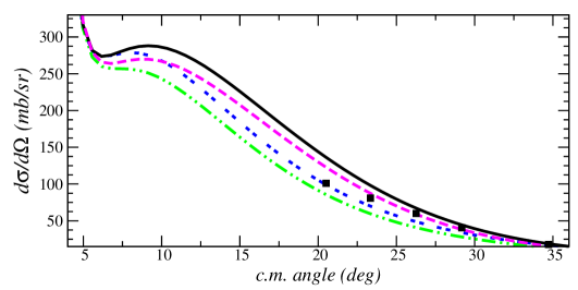
Figure 4: (color online) Same as Fig. 3 except that the angular distribution of the differential cross section ($\frac{d\sigma}{d\Omega}$) is plotted with a linear scale. The data are from Ref. Korsheninnikov:1997mm .

Let us first concentrate on the scattering of ⁶He at 71 MeV/nucleon. In Fig. 3 we show the differential cross section (upper panel (a)) and the analyzing power (lower panel (b)) for elastic scattering of ⁶He at 71 MeV/nucleon. For more detail we show the differential cross section in a linear scale in Fig. 4. The solid (black) line represents the calculation with a single-particle optical potential as outlined in Section II.B based on the COSMA density. On the log-scale of Fig. 3 the differential cross section looks reasonably well described. However, the linear scale of Fig. 4 reveals that a for the small angles, the single-particle optical potential over predicts the differential cross section. The analyzing power stays positive for all angles, similar to the predictions in Ref. Weppner:2000fi . Our calculation based on the cluster model using again the COSMA density is represented by the short-dashed (blue) line. The differential cross section is not very sensitive to the explicit cluster calculation with the exception of the forward angles, where the cluster calculation gives a lower cross section in better agreement with the data. The analyzing power, however, does not show any improvement though the minimum is slightly shifted to smaller angles, it stays positive, whereas the data indicate a negative sign. The folding for the optical potentials with the COSMA density are carried out with the free NN t-matrix as input. As has been shown in Ref. Chinn:1994xz for a variety of heavier nuclei, at energies lower than $\sim$150 MeV projectile energy, the free NN t-matrix experiences a modification due to the nuclear medium, which can be treated as an additional force represented by a mean field acting on the two active nucleons during the scattering process Chinn:1993zz . The dash-double-dotted (green) curves in Figs. 3 and 4 include a modification of the free NN t-matrix through an HFB mean field for the alpha cluster only. One advantage to this cluster paradigm is that the calculation can utilize the influence of a mean field on the free NN interaction where it is most appropriate, i.e. for the strongly bound $\alpha$-core. The results of this calculation produces an analyzing power, which turns negative at 60^o and captures the shape of the last two measured angles. However, it still over predicts the measured analyzing power at the smaller angles. The overall shape of the differential cross section is not modified. Only for the very forward angles the cross section is slightly lowered compared to the cluster calculation with the COSMA density as can be seen in Fig. 4.

It is further instructive to investigate the importance of the correlation density $\rho_{corr}({{\bf{\cal P}}_{j}}_{c})$ in Eq. (23) for the cluster optical potential. This can be done by realizing that setting $\rho_{corr}({{\bf{\cal P}}_{j}}_{c})=1$ omits the correlations. In Figs. 3 and 4 the dash-double-dotted (green) curve represents the calculation based on the cluster formulation whereas the short dashed (pink) line represent the same calculation with the correlation density set to 1. The effect on the analyzing power, Fig. 3, is relatively small. However, the differential cross section for small angles, Fig. 4, shows visible sensitivity. Indeed, one can conclude, that the lowering of the differential cross section for the forward angles is dominated by the influence of the correlation density.

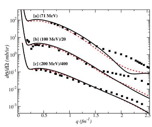
Figure 5: (color online) The angular distribution of the differential cross section ($\frac{d\sigma}{d\Omega}$) for elastic proton scattering off ⁴He at projectile energies 71 MeV, 100 MeV, and 200 MeV as function of the momentum transfer. The calculations are performed with optical potential based on the Nijmegen I potential Stoks:1993tb for the NN interaction. For the $\alpha$-core an HFB density according to Refs. HFB ; Gogny is employed. The solid lines (black) show the calculations based on the free NN t-matrix, while the dotted (red) lines are based on calculations modifying the NN t-matrix with a mean-field consistent with the HFB $\alpha$-core. The data are from Refs. Burzynski:1989zz ; Wesick:1986bt ; Comparat:1975bm ; Moss:1979aw .

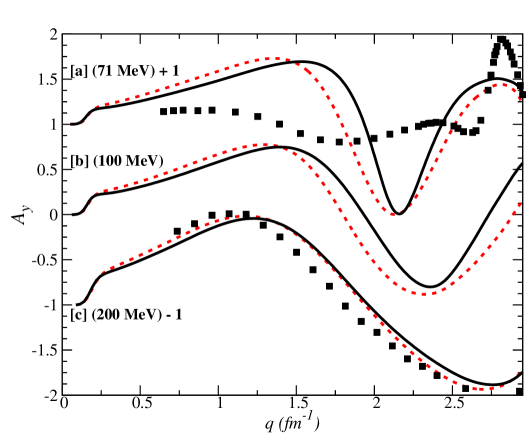
Figure 6: (color online) The angular distribution of the analyzing power for elastic proton scattering off ⁴He at projectile energies 71 MeV, 100 MeV, and 200 MeV as function of the momentum transfer. The meaning of the curves is the same as in Fig. 5. The data are from Refs. Burzynski:1989zz ; Wesick:1986bt ; Comparat:1975bm ; Moss:1979aw .

The upgrade of the RIKEN facility will in principle allow to measure the angular distribution of the analyzing power for the elastic scattering of ⁶He at somewhat higher energies. Thus we want to investigate the predictions for the elastic scattering observables as function of the projectile energy using a cluster ansatz for the optical potential for ⁶He. As test energies we choose 100 MeV and 200 MeV/nucleon. First, we show in Figs. 5 and 6 the angular distributions of the differential cross section and the analyzing power for proton scattering off ⁴He as function of the momentum transfer. The calculations for the projectile energy of 200 MeV shows that here an optical potential description of the scattering process is quite good up to 2.5 fm^-1 for both, differential cross section and analyzing power. In Figs. 5 and 6 two calculations are shown: For the solid line a folding calculation of the optical potential has been carried out using the free NN t-matrix, whereas for the dashed line a NN t-matrix modified by a HFB mean field has been used. At 200 MeV a folding with the free NN t-matrix is adequate. At the two lower energies, a single scattering optical potential describes the differential cross section only up to a momentum transfer of about 1.75 fm^-1. For higher momentum transfers multiple scattering contributions are expected to become important. However, only for a deuteron target multiple scattering contributions have been investigated systematically Liu:2004tv ; Elster:2008yt over a wide range of projectile energies. Thus, we can only speculate about the increasing importance of multiple scattering contributions at higher momentum transfer. The analyzing power at 71 MeV projectile energy is not well described for small momentum transfers. This is very likely the reason for our over-prediction of the analyzing power of ⁶He for small momentum transfer at this energy Sakaguchi:2011rp .

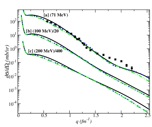
Figure 7: (color online) The angular distribution of the differential cross section ($\frac{d\sigma}{d\Omega}$) for elastic scattering of ⁶He at projectile energies 71 MeV, 100 MeV, and 200 MeV/nucleon as function of the momentum transfer. The calculations are performed with optical potential based on the Nijmegen I potential Stoks:1993tb for the NN interaction. For the solid (black) line the COSMA Zhukov:1994zz has been used as single-particle density. The short-dashed (blue) line incorporated the cluster structure into the optical potential using the COSMA density for all clusters. For the dash-double-dot (green) line the free NN t-matrix has been modified with the HFB mean field. The data are taken from Ref. Uesaka:2010mm ; Korsheninnikov:1997mm .

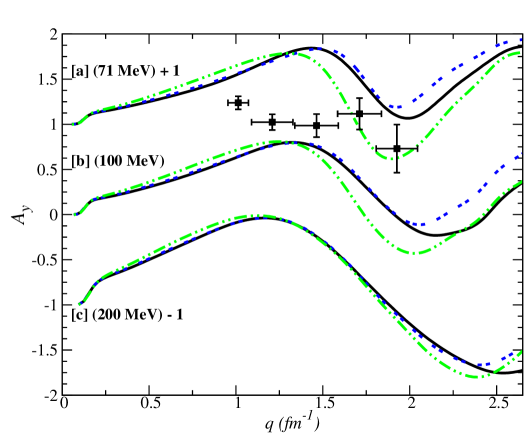
Figure 8: (color online) The angular distribution of the the analyzing power ($A_{y}$) for elastic scattering ⁶He at projectile energies 71 MeV, 100 MeV, and 200 MeV/nucleon as function of the momentum transfer. The meaning of the lines is the same as in Fig. 7. The data are taken from Ref. Uesaka:2010mm ; Korsheninnikov:1997mm .

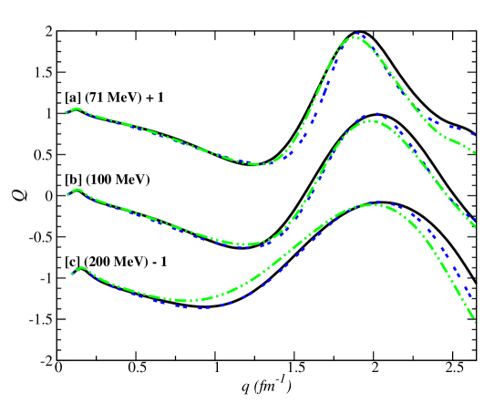
Figure 9: (color online) The angular distribution of the the spin rotation function $Q$ for elastic scattering ⁶He at projectile energies 71 MeV, 100 MeV, and 200 MeV/nucleon as function of the momentum transfer. The meaning of the lines is the same as in Fig. 7.

In Figs. 7 and 8 we present predictions for elastic scattering of ⁶He at 100 MeV and 200 MeV/nucleon. The solid lines represent the calculations with a single-particle optical potential, whereas the short-dashed and dash-double dotted lines are based on the cluster formulation discussed in Section II.C. The short-dashed line uses a free NN t-matrix for every piece of the optical potential, whereas the dash-double-dotted line incorporates a NN t-matrix modified by an HFB mean field potential for the $\alpha$-core. Similar to the ⁴He calculations, at 200 MeV/nucleon the modification of the NN t-matrix becomes irrelevant. As discussed for the 71 MeV/nucleon calculations, the cluster model lowers the predictions for the differential cross section for small momentum transfers (angles). This feature seems independent of the employed projectile energy. For the analyzing power at small momentum transfer the contribution of the valence neutrons is not large enough to change the contribution of the $\alpha$-core part of the optical potential. For the 100 MeV calculation the modification of the free NN t-matrix through the nuclear medium is still quite pronounced at $\sim$2 fm^-1 momentum transfer, whereas the 200 MeV/nucleon calculations exhibit very little difference between each other. In Fig. 9 we show the spin-rotation function $Q$ for elastic scattering of ⁶He at the same energies. Obviously, this observable has no chance of being measured. However, since it is an independent observable, we consider it instructive to study if it exhibits differences similar to the ones in the analyzing power between a cluster paradigm for the optical potential and a single-particle optical potential. It is interesting to note, that $Q$ is very insensitive to any of the modifications introduced, even at 71 MeV/nucleon.

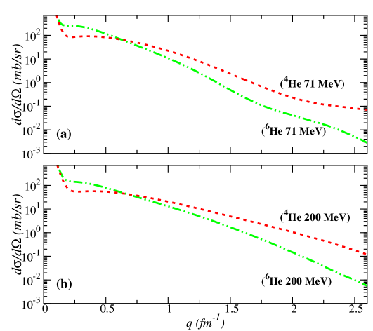
Figure 10: (color online) The angular distribution of the differential cross section, $\frac{d\sigma}{d\Omega}$, for elastic proton scattering off ⁴He (short-dashed red) and ⁶He (dash-double-dot green) at projectile energies 71 MeV (upper panel (a)) and 200 MeV/nucleon (lower panel (b)) as function of the momentum transfer. Both calculations are performed with optical potential based on the Nijmegen I potential Stoks:1993tb for the NN interaction, which for ⁴He (in the ⁶He case the ⁴He-core) is modified by the HFB mean field. For the ⁶He calculations the single particle nucleons are described by the COSMA density, and the cluster ansatz is used. For the ⁴He calculations the HFB density HFB ; Gogny is employed.

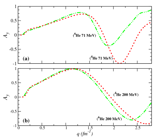
Figure 11: (color online) The angular distribution of the analyzing power for elastic proton scattering off ⁴He (short-dashed red) and ⁶He (dash-double-dot green) at projectile energies 71 MeV (upper panel (a)) and 200 MeV/nucleon (lower panel (b)) as function of the momentum transfer. The meaning of the curves is the same as in Fig. 10.

In order to investigate if the difference of the observables for elastic scattering of ⁴He and ⁶He changes with increasing energy, we plot in Figs. 10 and 11 the differential cross sections and analyzing powers for the two nuclei together at 71 MeV and 200 MeV as function of the momentum transfer. One could speculate that when employing a cluster model for the ⁶He nucleus, at higher energies the piece of the optical potential due to the $\alpha$-core might dominate the observables (possibly the analyzing power). However, this does not seem to be the case, the behavior of the differential cross section is very similar at the two energies. Even the shift of the minima in the analyzing power between the two nuclei is the same for both energies, namely roughly 0.25 fm^-1. Obviously, experimental information will have to decide if a cluster ansatz as presented here captures a major part of the underlying physics.

IV Summary and Outlook

In this work we introduced a cluster formulation for the optical potential for calculating scattering observables for elastic scattering of three-body halo nuclei. We first reviewed a traditional single-particle full-folding optical potential in first order in the Watson multiple scattering expansion, and then showed how one can naturally extend this optical potential to introduce the cluster structure of a halo nucleus. Here we concentrate on the ⁶He nucleus. However, the formulation we introduced can be further extended to four or five-body clusters, e.g. to ⁸He. For our calculations we used the density matrix of the three-body cluster orbital shell model approximation (COSMA) introduced in Refs. Zhukov:1994zz ; Zhukov:1991 for the ⁶He nucleus. This density matrix is based on single harmonic oscillator wave functions for the s- and p-shell of ⁶He and allows a straightforward calculation of the required correlation densities needed for the optical potential. The resulting folding optical potential contains a six dimensional integration over internal vector momenta, which is calculated via Monte Carlo integration.

We calculated the angular distribution of the differential cross section and the analyzing power at 71 MeV, 100 MeV, and 200 MeV/nucleon and compared our results with experimental data at 71 MeV/nucleon Uesaka:2010mm ; Korsheninnikov:1997mm . We find that the cluster model lowers the cross section for the small angles and brings it closer to the data. Though we do not describe the very small analyzing power at the small angles, we find that the cluster formulation together with a ‘hybrid’ ansatz, in which the optical potential for the alpha-core is calculated with a NN t-matrix modified by a mean field of the alpha is able to produce a negative analyzing power at larger angles as suggested by the data. Our predictions for the higher energies indicate that the lowering of the differential cross section for small momentum transfers (angles) using a cluster paradigm remains visible. The cluster ansatz for the optical potential continues to predict a negative analyzing power at larger momentum transfer. Eventually experimental information should be become available to see if these predictions capture the bulk of the physics of the reaction at higher energies, or if there are additional theoretical pieces necessary to understand this reaction, preferably as function of scattering energy.

Appendix A First Order Full-Folding Optical Potential

In this appendix we will give explicit steps for arriving at the ‘traditional’ first order Watson optical potential of our calculations. The complete derivation is given in Ref. Elster:1997as , however for the convenience of the reader we want to give a shorter summary here.

Using the $\delta$-function of Eq. (14), which determines the conservation of the absolute momentum for the center of mass (c.m.) frame of the nucleus and the relative momenta of the individual nucleons in the target, we obtain for the optical potential of Eq. (13)

$$\langle\hat{\tau}_{01}\rangle \equiv \langle{\bf k^{\prime}}|\langle\phi_{A}|{\hat{\tau}}_{0i}{(\cal{E}})|\phi_{A}\rangle|{\bf k}\rangle$$ (28)

$$= \int\prod_{j=1}^{A}d{\bf{k}}_{j}^{\prime}\;\int\prod_{l=1}^{A}d{\bf{k}}_{l}\;\langle\phi_{A}|{\bf{\zeta}}_{1}^{\prime}{\bf{\zeta}}_{2}^{\prime}{\bf{\zeta}}_{3}^{\prime}{\bf{\zeta}}_{4}^{\prime}...{\bf{\zeta}}_{A-1}^{\prime}\rangle\delta({\bf{p}}^{\prime}-{\bf{p}}_{0}^{\prime})\;\langle{\bf{k}}^{\prime}{\bf{k}}_{1}^{\prime}|\hat{\tau}_{01}({\cal{E}})|{\bf{k}}{\bf{k}}_{1}\rangle$$ (30)

$$\prod_{j=2}^{A}\delta({\bf{k}}_{j}^{\prime}-{\bf{k}}_{j})\delta({\bf{p}}-{\bf{p}}_{0})\;\langle{\bf{\zeta}}_{1}{\bf{\zeta}}_{2}{\bf{\zeta}}_{3}{\bf{\zeta}}_{4}...{\bf{\zeta}}_{A-1}|\phi_{A}\rangle,$$

where ${\bf{p}}=\sum_{i=1}^{A}{\bf{k}}_{i},{\bf{p}}^{\prime}=\sum_{i=1}^{A}{\bf{k}}^{\prime}_{i}$. Without losing generality, we consider for now nucleon ‘$1$’ being the active nucleon in the target. The additional delta functions arises because the target nucleons are independent of $\hat{\tau}_{01}$. A Galilean invariant choice of internal variables are the Jacobi coordinates,

$${\bf{k}}_{1} = {\bf\zeta_{1}}+\frac{{\bf{p}}}{A}$$

$${\bf{k}}_{2} = {\bf\zeta_{2}}-\frac{{\bf\zeta_{1}}}{A-1}+\frac{{\bf{p}}}{A}$$

$${\bf{k}}_{3} = {\bf{\bf\zeta_{3}}}-\frac{{\bf\zeta_{1}}}{A-1}-\frac{\bf\zeta_{2}}{A-2}+\frac{{\bf{p}}}{A}$$

$$\vdots$$

$${\bf{k}}_{A} = {\bf\zeta_{A}}-\sum_{j=1}^{A-1}\frac{\bf\zeta_{j}}{A-j}+\frac{{\bf{p}}}{A}.$$ (31)

In first order, which is the concern of this work, we only need the momentum of the struck nucleon, namely ${\bf{k}}_{1}={\bf\zeta_{1}}+\frac{{\bf{p}}}{A}$. Changing integration variables from absolute to relative momenta in Eq. (30) results in

$$\langle\hat{\tau}_{01}\rangle = \;\int\prod_{j=1}^{A-1}d{\bf\zeta_{j}^{\prime}}d{\bf{p}}^{\prime}\;\int\prod_{l=1}^{A-1}d{\bf\zeta_{l}}d{\bf{p}}\;\langle\phi_{A}|{\bf\zeta_{1}^{\prime}\zeta_{2}^{\prime}\zeta_{3}^{\prime}\zeta_{4}^{\prime}...{\bf{\zeta}}_{A-1}^{\prime}}\rangle\delta({\bf{p}}^{\prime}-{\bf{p}}^{\prime}_{0})$$ (32)

$$\langle{\bf{k}}^{\prime},{\bf\zeta_{1}^{\prime}}+\frac{{\bf{p}}^{\prime}}{A}|\hat{\tau}_{01}({\cal{E}})|{\bf{k}},{\bf\zeta_{1}}+\frac{{\bf{p}}}{A}\rangle\prod_{j=2}^{A-1}\delta({\bf\zeta_{j}^{\prime}}-{\bf\zeta_{j}})\delta\left(\frac{A-1}{A}{\bf{p}}^{\prime}-{\bf\zeta_{1}^{\prime}}-\frac{A-1}{A}{\bf{p}}+{\bf\zeta_{1}}\right)$$

$$\delta({\bf{p}}-{\bf{p}}_{0})\langle{\bf\zeta_{1}\zeta_{2}\zeta_{3}\zeta_{4}...\zeta_{A-1}}|\phi_{A}\rangle.$$

Eq. (32) indicates that one only needs the single particle density matrices $\rho({\bf\zeta_{1}^{\prime},\zeta_{1}})$, describing the dependence of one particle’s relative motion to the remaining (A-1)-core, and given in Eq. (15). Inserting $\rho({\bf\zeta_{1}^{\prime}},{\bf\zeta_{1}})$ into Eq. (32) and evaluating $\delta({\bf{p}}-{\bf{p}}_{0})$ and $\delta({\bf{p}}^{\prime}-{\bf{p}}^{\prime}_{0})$ leads to

$$\langle\hat{\tau}_{01}\rangle = \;\int d{\bf\zeta_{1}^{\prime}}\;\int d{\bf\zeta_{1}}\langle{\bf{k}}^{\prime}\;{\bf\zeta_{1}^{\prime}}+\frac{{\bf{p}}_{0}^{\prime}}{A}\left|\hat{\tau}_{01}({\cal{E}})\right|{\bf{k}}\;{\bf\zeta_{1}}+\frac{{\bf{p}}_{0}}{A}\rangle\;\rho({\bf\zeta_{1}^{\prime},{\bf{\zeta}}_{1}})$$ (33)

$$\;\delta\left(\frac{A-1}{A}{\bf{p}}_{0}^{\prime}-{\bf\zeta_{1}^{\prime}}-\frac{A-1}{A}{\bf{p}}_{0}+{\bf\zeta_{1}}\right).$$

Inserting the NN ${\hat{\tau}}_{01}$-matrix of Eq. (eq:2.8.1c) and taking advantage of its conservation of the c.m. momentum Eq. (33) becomes

$$\langle\hat{\tau}_{01}\rangle = \;\int d{\bf\zeta_{1}^{\prime}}\;\int d{\bf\zeta_{1}}\;\delta({\bf{k}}^{\prime}+{\bf{p}}_{0}^{\prime}-{\bf{k}}-{\bf{p}}_{0})$$ (34)

$$\left\langle\frac{1}{2}({\bf{k}}^{\prime}-{\bf\zeta_{1}^{\prime}}-\frac{{\bf{p}}_{0}^{\prime}}{A})|\hat{\tau}_{01}({\cal{E}})|\frac{1}{2}({\bf{k}}-{\bf\zeta_{1}}-\frac{{\bf{p}}_{0}}{A})\right\rangle\;\;\rho({\bf\zeta_{1}^{\prime}},{\bf\zeta_{1}})$$

$$\delta\left(\frac{A-1}{A}{\bf{p}}_{0}^{\prime}-{\bf\zeta_{1}^{\prime}}-\frac{A-1}{A}{\bf{p}}_{0}+{\bf\zeta_{1}}\right).$$

The first delta function describes the overall momentum conservation, which can be used to reduce the integral of Eq. (34) to three dimensions, i.e. the integral given in Eq. (17). In our practical calculations we use the variables ${\bf{q}}$, ${\bf{K}}$, and ${\bf{P}}$, which are given in Eq. (19). The inverse relations are given by

$${\bf{k}} = {\bf{K}}-\frac{1}{2}{\bf{q}}$$

$${\bf{k}}^{\prime} = {\bf{K}}+\frac{1}{2}{\bf{q}}$$

$${\bf{\zeta}}_{1} = {\bf{P}}+\frac{A-1}{2A}{\bf{q}}$$

$${\bf{\zeta}}_{1}^{\prime} = {\bf{P}}-\frac{A-1}{2A}{\bf{q}}.$$ (35)

Substituting those variables into Eq. (17) leads to

$$\langle\hat{\tau}_{01}\rangle = \left\langle\frac{1}{2}\left({\bf{K}}-{\bf{P}}+\frac{2A-1}{2A}{\bf{q}}-\frac{{\bf{p}}_{0}^{\prime}}{A}\right)|\hat{\tau}_{01}({\cal{E}})|\frac{1}{2}\left({\bf{K}}-{\bf{P}}-\frac{2A-1}{2A}{\bf{q}}-\frac{{\bf{p}}_{0}}{A}\right)\right\rangle\;$$ (36)

$$\rho\left({\bf{P}}-\frac{A-1}{2A}{\bf{q}},{\bf{P}}+\frac{A-1}{2A}{\bf{q}}\right).$$

Here we dropped the overall momentum conserving delta function, which is carried out when evaluating the cross section. Since the preceding derivation based on the projectile particle ‘0’ and active target particle ‘1’ is general, and thus can be repeated for all $N$ target neutrons and $Z$ target protons, one obtains as final expression for the ‘full-folding’ optical potential

$$U_{el}\left({\bf{K}}+\frac{1}{2}{\bf{q}},{\bf{K}}-\frac{1}{2}{\bf{q}}\right)=$$ (38)

$$\sum_{i=N,P}\;\int d{\bf{P}}\left\langle\frac{1}{2}\left({\bf{K}}-{\bf{P}}+\frac{2A-1}{2A}{\bf{q}}-\frac{{\bf{p}}_{0}^{\prime}}{A}\right)|\hat{\tau}_{0i}({\cal{E}})|\frac{1}{2}\left({\bf{K}}-{\bf{P}}-\frac{2A-1}{2A}{\bf{q}}-\frac{{\bf{p}}_{0}}{A}\right)\right\rangle\;$$

$$\rho_{i}\left({\bf{P}}-\frac{A-1}{2A}{\bf{q}},{\bf{P}}+\frac{A-1}{2A}{\bf{q}}\right).$$

From Eq. (38) we can read off the momenta of the NN t-matrix as

$${\bf{k}}_{NN} = \frac{1}{2}\left({\bf{K}}-{\bf{P}}-\frac{2A-1}{2A}{\bf{q}}-\frac{{\bf{p}}_{0}}{A}\right)$$

$${\bf{k}}_{NN}^{\prime} = \frac{1}{2}\left({\bf{K}}-{\bf{P}}+\frac{2A-1}{2A}{\bf{q}}-\frac{{\bf{p}}_{0}^{\prime}}{A}\right).$$ (39)

For numerical calculations we prefer

$${\bf{q}}_{NN} = {\bf{k}}_{NN}^{\prime}-{\bf{k}}_{NN}={\bf{k}}^{\prime}-{\bf{k}}={\bf{q}}$$

$${\bf{K}}_{NN} = \frac{1}{2}\left({\bf{k}}_{NN}^{\prime}+{\bf{k}}_{NN}\right)=\frac{1}{2}\left({\bf{K}}-{\bf{P}}-\frac{{\bf{p}}_{0}+{\bf{p}}_{0}^{\prime}}{2A}\right).$$ (40)

Since $\bf{q}$ is a momentum transfer, it is invariant under Galilean transformations, i.e. ${\bf{q}}_{NN}={\bf{q}}$. Rewriting the optical potential in terms of q and K gives

$$U_{el}({\bf{q}},{\bf{K}})=$$ (42)

$$\sum_{i=N,P}\int d{\bf{P}}\hat{\tau}_{0i}\left({\bf{q}},\frac{1}{2}\left({\bf{K}}-{\bf{P}}-\frac{{\bf{p}}_{0}+{\bf{p}}_{0}^{\prime}}{2A}\right),{\cal{E}}\right)\;\rho_{i}\left({\bf{P}}-\frac{A-1}{2A}{\bf{q}},{\bf{P}}+\frac{A-1}{2A}{\bf{q}}\right).$$

Rewriting Eq. (42) in variables of the NA c.m. system requires that ${\bf{k}}+{\bf{p}}_{0}={\bf{k}}^{\prime}+{\bf{p}}_{0}^{\prime}=0$. Thus, the dependence of ${\bf{p}}_{0}$ drops out, and one obtains for the ‘full-folding’ single-particle optical potential of Eq. (21)

$$U_{el}({\bf{q}},{\bf{K}})=$$ (44)

$$\sum_{i=n,p}\int d{\bf{P}}\hat{\tau}_{0i}\left({\bf{q}},\frac{1}{2}\left(\frac{A+1}{A}{\bf{K}}-{\bf{P}}\right),{\cal{E}}\right)\;\rho_{i}\left({\bf{P}}-\frac{A-1}{2A}{\bf{q}},{\bf{P}}+\frac{A-1}{2A}{\bf{q}}\right).$$

Appendix B Transforming the optical potential

We first want to calculate the optical potential for a nucleon scattering off a cluster ‘$i$’ in the c.m. frame of the projectile and the cluster ‘$i$’ (e.g. cluster ‘$i$’ could be the $\alpha$ particle within the ⁶He nucleus). Let us use the subscript $C_{i}$ to denote that frame, whereas quantities without subscripts shall be interpreted as given in the $A+1$ c.m. frame. The overall conservation of momentum for the c.m. cluster frame assumes

$${\bf{k}}_{C_{i}}+{\bf{k_{1}}}_{C_{i}}={{{\bf{k}}^{\prime}}_{C_{i}}}+{\bf{{k^{\prime}_{1}}_{C_{i}}}}\equiv 0,$$ (45)

where ${\bf{k}}_{C_{i}}$ is the projectile and ${\bf{k_{1}}}_{C_{i}}$ is a typical target nucleon inside the nucleus, within the $i$th cluster.

Starting with the definition of the density given in Eq. (31) in the $A+1$ frame,

$${\mathbf{\zeta}_{1}}={\bf{k}}_{1}-\frac{{\bf{p}}}{A},$$

this becomes in a specific cluster frame

$${\mathbf{\zeta}_{1}}={\bf{k_{1}}}_{C_{i}}-\frac{{\bf{p}}_{C_{i}}}{A}.$$ (46)

The momentum ${\mathbf{\zeta}_{1}}$ does not carry a cluster subscript since it is defined in the traditional intrinsic frame of the single particle density. Eq. (46) defines how this intrinsic variable is related via a Galilean transformation to the cluster frame. Using the notation of Eq. (22), this can be broken up into the active particle and the spectator

$${\mathbf{\zeta}_{1}}={\bf{k_{1}}}_{C_{i}}-\frac{{\bf{p_{i}}}_{C_{i}}+{\bf{{p_{s}}_{i}}}_{C_{i}}}{A}.$$ (47)

In this center of mass frame one has ${\bf{k}}_{C_{i}}=-{\bf{p_{i}}}_{C_{i}}$, where ${\bf{k}}_{C_{i}}$ is the momentum of the projectile in the cluster frame. Then using Eq. (47), this result together with understanding that the spectator momentum does not change during the collision, we can calculate the difference

$${\bf\zeta_{1}}-{{\bf\zeta_{1}}}^{\prime}=({\bf{k_{1}}}_{C_{i}}-{{\bf{k_{1}^{\prime}}}_{C_{i}}})-(\frac{{{\bf{k^{\prime}}}_{C_{i}}}-{\bf{k}}_{C_{i}}}{A})=\frac{A-1}{A}{\bf{q}},$$ (48)

remembering that ${\bf{q}}$, the relative momentum transfer, is invariant in all frames. If we allow the same definition for the average momentum of the target nucleon, Eq. (19)

$${\bf{P}}\equiv\frac{1}{2}({\bf{\zeta_{1}}}^{\prime}+{\bf\zeta_{1}}),$$ (49)

then the inverse equations of Eq. (35),

$${\bf\zeta_{1}}={\bf{P}}+\frac{A-1}{2A}{\bf{q}}$$

$${\bf{\zeta_{1}}}^{\prime}={\bf{P}}-\frac{A-1}{2A}{\bf{q}}$$ (50)

have the same form. This makes sense, since ${\bf{q}}$ is invariant and ${\bf{P}}$ is written in the intrinsic frame of the nucleus.

The momentum arguments of the $\hat{\tau}_{0i}$-matrix are defined in Eq. (39) for the $A+1$ frame. However, we also need to redefine them in the cluster frame $C_{i}$. Rewriting Eq. (39) and using Eqs. (47) and (50), we can write the relative momentum between the projectile, ${\bf{k}}_{C_{i}}$ and the struck nucleon, ${\bf{k_{1}}}_{C_{i}}$ as

$${\bf{k}}_{C_{i}}-{\bf{k_{1}}}_{C_{i}}={\bf{k_{NN}}}_{C_{i}}={\bf{k}}_{C_{i}}-{\bf\zeta_{1}}+\frac{{\bf{k}}_{C_{i}}-{\bf{{p_{s}}_{i}}}_{C_{i}}}{A}.$$ (51)

The primed momentum is similarly given as

$${\bf{k^{\prime}_{C_{i}}}}-{\bf{{k^{\prime}_{1}}_{C_{i}}}}={\bf{{k^{\prime}_{NN}}_{C_{i}}}}={\bf{k^{\prime}_{C_{i}}}}-{{\bf\zeta_{1}}}^{\prime}+\frac{{\bf{{k^{\prime}}_{C_{i}}}}-{\bf{{{p^{\prime}_{s}}_{i}}_{C_{i}}}}}{A}.$$ (52)

The difference between Eq. (51) and Eq.(52) gives the momentum transfer ${\bf{q}}$ as expected. We can define the sum of the momenta of the $\hat{\tau}_{0i}$-matrix as the sum of Eqs. (51) and (52) as

$${\bf{K_{NN}}}_{C_{i}}=\frac{{\bf{k_{NN}}}_{C_{i}}+{\bf{{k^{\prime}_{NN}}_{C_{i}}}}}{2}=\frac{A+1}{2A}({\bf{k_{C_{i}}}}+{\bf{k^{\prime}_{C_{i}}}})-\frac{1}{2}({\bf\zeta_{1}}+{{\bf\zeta_{1}}}^{\prime})-\frac{{\bf{{p_{s}}_{i}}}_{C_{i}}}{A},$$ (53)

remembering that the spectator momentum does not change during the collision. In the spirit of Eq. (19) we can define the sum of the cluster momenta as ${\bf{K}}_{C_{i}}=\frac{1}{2}({{\bf{k_{NN}}}_{C_{i}}+{\bf{{k^{\prime}_{NN}}_{C_{i}}}}})$ and then rewrite Eq. (53) as

$${\bf{K_{NN}}}_{C_{i}}=\frac{{\bf{k_{NN}}}_{C_{i}}+{\bf{{k^{\prime}_{NN}}_{C_{i}}}}}{2}=\frac{A+1}{A}{\bf{K}}_{C_{i}}-{\bf{P}}-\frac{{\bf{{p_{s}}_{i}}}_{C_{i}}}{A}.$$ (54)

Examining Eqs. (39) through (21), we see that the momentum argument ${\bf{K_{NN}}}$ of the $\hat{\tau}_{0i}$-matrix has picked up an extra term involving the spectator momentum in the cluster frame. The rational for this is simple, the struck nucleon is acted upon in a specific cluster, but the total density contains both cluster and spectators.

We can rewrite ${\bf{K_{NN}}}$ in terms of the correlation momentum ${{\bf{\cal P}}_{j}}_{i}$ by multiplying ${\bf{K_{NN}}}_{C_{i}}$ by the number of nucleons in the $i$th cluster, $A_{i}$,

$${\bf{A}}_{i}{K_{NN}}_{C_{i}}=A_{i}\frac{A+1}{A}{\bf{K}}_{C_{i}}-A_{i}{\bf{P}}-A_{i}\frac{{\bf{{p_{s}}_{i}}}_{C_{i}}}{A}.$$ (55)

After some manipulation as well as using the definition of ${{\bf{\cal P}}_{j}}_{i}$ found in Eq. (23), one finds

$${\bf{A}}_{i}{K_{NN}}_{C_{i}}=(A_{i}+1){\bf{K}}_{C_{i}}-A_{i}{\bf{P}}+{{\bf{\cal P}}_{j}}_{i},$$ (56)

so a cleaner definition of the average momentum can be written as

$${K_{NN}}_{C_{i}}=\frac{A_{i}+1}{A_{i}}{\bf{K}}_{C_{i}}-{\bf{P}}+\frac{{{\bf{\cal P}}_{j}}_{i}}{A_{i}}.$$ (57)

Thus, for a specific cluster frame we can write the optical potential as

$${U_{el}({\bf{q}},{\bf{K}})}_{C_{i}}=\sum_{t=n,p}\int d{\bf{P}}\;d{{\bf{\cal P}}_{j}}_{i}\;\rho_{corr}({{\bf{\cal P}}_{j}}_{i})$$ (59)

$$\hat{\tau}_{0t}\left({\bf{q}},\frac{1}{2}\left(\frac{A_{i}+1}{A_{i}}{\bf{K}}_{C_{i}}-{\bf{P}}+\frac{{{\bf{\cal P}}_{j}}_{i}}{A_{i}}\right),{\cal{E}}\right)\;\rho_{i}\left({\bf{P}}-\frac{A-1}{2A}{\bf{q}},{\bf{P}}+\frac{A-1}{2A}{\bf{q}}\right).$$

In the case of ⁶He this is the optical potential for a proton on the alpha core (or the proton projectile on one of the neutrons). We have not worried about the correlation density transformation since this is based on a relative momentum ${{\bf{\cal P}}_{j}}_{i}$ and is thus invariant during a frame transformation, as are ${\bf{P}}$ and ${\bf{q}}$, the variables of the traditional single particle density.

In order to be useful, Eq. (59) must be transformed from each individual cluster frame back to the nucleon-nucleus frame, so that it can be summed with the other clusters which make up the target nucleus. Scattering observables can then be calculated in the c.m. frame of the $A+1$ system following Eq. (27). As it stands, each cluster has its own unique c.m. frame, and thus they cannot be summed until they are transformed back to the unique $A+1$ c.m. frame. The only argument of concern, because it is not invariant, is the momentum ${\bf{K}}_{C_{i}}$ in the $\hat{\tau}_{0i}$ operator.

Employing conservation of momentum in both frames, we can define how the cluster frame relates to the nucleon-nucleus $A+1$ frame. Setting relative velocities equivalent in the two different frames leads to

$$A_{i}{\bf k}-{\bf p_{i}}=A_{i}{\bf k}_{C_{i}}-{\bf{p_{i}}}_{C_{i}}=(A_{i}+1){\bf k}_{C_{i}},$$ (60)

where the last equivalence is given because in the c.m. of the cluster frame ${\bf k}_{C_{i}}=-{\bf p_{i}}_{C_{i}}$. Another second relation between the two frames is gained by examining the Jacobi momentum of Eq. (22) in the $A+1$ frame,

$${{\bf{p}}_{j}}_{i}=\frac{1}{A}({A_{s}}_{i}{\bf{p}}_{i}-A_{i}{\bf{p_{s}}}_{i}).$$ (61)

Rearranging gives

$${\bf{p}}_{i}=\frac{A_{i}}{A}\left({\bf{p}}_{i}+{\bf{p_{s}}}_{i}\right)+{{\bf{p}}_{j}}_{i}=-\frac{A_{i}}{A}{{\bf{k}}}+{{\bf{p}}_{j}}_{i},$$ (62)

where again the last equivalence is found by recognizing that in the $A+1$ frame the c.m. momentum is defined as ${\bf{k}}+{\bf{p}}_{i}+{\bf{p_{s}}}_{i}=0$. Inserting the result for ${\bf{p}}_{i}$ from Eq. (62) into Eq. (60) we can after some manipulation compare the momenta between the two frames:

$${\bf{k}}=\frac{A}{A+1}\frac{1}{A_{i}}\left((A_{i}+1)k_{C_{i}}+{{\bf{p}}_{j}}_{i}\right).$$ (63)

The same relationship can be developed for the primed momentum

$${\bf{k}}^{\prime}=\frac{A}{A+1}\frac{1}{A_{i}}\left((A_{i}+1){{\bf k}^{\prime}_{C_{i}}}+{{{\bf{p}}_{j}^{\prime}}_{i}}\right).$$ (64)

Adding these two equations gives

$${\bf{K}}=\frac{A}{A+1}\frac{1}{A_{i}}\left((A_{i}+1){\bf K}_{C_{i}}+{{\bf{\cal P}}_{j}}_{i}\right).$$ (65)

This relation is the transformation prescription for $K$ from the cluster frame to the $A+1$ frame. Solving for ${\bf K}_{C_{i}}$ in Eq. (65) and plugging it into the optical potential in the cluster frame of Eq. (59) we are then able to express this potential completely using invariants or nucleon-nucleus $A+1$ variables,

$${U_{el}({\bf{q}},{\bf{K}})}_{C_{i}} = \sum_{t=n,p}\int d{\bf{P}}\;d{{\bf{\cal P}}_{j}}_{i}\;\rho_{corr}({{\bf{\cal P}}_{j}}_{i})$$ (66)

$$\hat{\tau}_{0t}\left({\bf{q}},\frac{1}{2}\left(\frac{A+1}{A}{\bf{K}}-{\bf{P}}\right),{\cal{E}}\right)\;\rho_{i}\left({\bf{P}}-\frac{A-1}{2A}{\bf{q}},{\bf{P}}+\frac{A-1}{2A}{\bf{q}}\right).$$

This is Eq. (27) from Section II.C for the cluster optical potential in the nucleon-nucleus frame.

Appendix C Correlation Density for the Cluster Approach

The cluster approach developed in this work uses a correlation density relating the clusters, which is given in Eq. (23),

$$\rho_{corr}({{\bf{p}}_{j}}_{1},{{\bf{p}}^{\prime}_{j}}_{1})\equiv\int\prod_{l=2}^{N_{c}}d{{{\bf{p}}^{\prime}_{j}}_{l}}\int\prod_{m=2}^{N_{c}}d{{{\bf{p}}_{j}}_{m}}\langle\phi_{A}|{\bf{p^{\prime}_{j}}}_{1}{\bf{p^{\prime}_{j}}}_{2}...{\bf{p^{\prime}_{j}}}_{N_{c}}\rangle\;\langle{\bf{p_{j}}}_{1}{\bf{p_{j}}}_{2}...{\bf{p_{j}}}_{N_{c}}|\phi_{A}\rangle,$$ (67)

This density correlates the momenta between the various clusters and elevates the this approach beyond the independent single particle picture. For the explicit derivation, let us start from definition given in Eq. (22)

$${{\bf{p}}_{j}}_{i}=\frac{1}{A}({A_{s}}_{i}{\bf{p}}_{i}-A_{i}{\bf{p_{s}}}_{i}).$$ (68)

This definition is invariant from the frame of consideration. Thus it can be applied in the frame of the intrinsic density, where it describes the difference in momenta between cluster $i$ and its analogous spectator particles, ${\bf{p_{s}}}_{i}$, in the laboratory frame. In this same frame the total momentum between active and spectator particles should add up to zero, at least before the collision. Thus, ${\bf{p}}_{i}=-{\bf{p_{s}}}_{i}$, and therefore ${{\bf{p}}_{j}}_{i}={\bf{p}}_{i}$ and ${{{\bf{p}}_{j}}_{i}}^{\prime}={\bf{p}}_{i}-{\bf{q}}$. Again, in the intrinsic frame of the nucleus one has

$${{\bf{\cal P}}_{j}}_{i}=\frac{{{\bf{p}}_{j}}_{i}+{{\bf{p}}_{j}}^{\prime}_{i}}{2}={{{\bf{p}}_{j}}_{i}}-\frac{{\bf{q}}}{2}.$$ (69)

For the ⁶He nucleus consisting of three clusters, we can write the correlation density as

$$\rho_{corr}({{\bf{p}}_{j}}_{1},{{\bf{p}}^{\prime}_{j}}_{1})\equiv$$ (71)

$$\int d^{3}{{\bf{p}}_{s_{i}}}_{1}d({\bf{\hat{z}}}\cdot{\bf{\hat{p}_{i}}})\;d^{3}{{{\bf{p}}^{\prime}_{s_{i}}}_{1}}\;d^{3}{{\bf{p}}_{s_{i}}}_{2}\;d^{3}{{{\bf{p}}^{\prime}_{s_{i}}}_{2}}\;\;\Phi({{\bf{p}}_{s_{i}}}_{1})\;\Phi({{\bf{p}}_{s_{i}}}_{2})\;\Phi({{{\bf{p}}^{\prime}_{s_{i}}}_{1}})\;\Phi({{{\bf{p}}^{\prime}_{s_{i}}}_{2}})$$

$$f_{corr}({\bf{\Omega}}_{s_{1}},{\bf{\Omega}}_{s_{2}})\delta({\bf{p_{i}}}-{\bf{p_{s_{i}}}}_{1}-{\bf{i}}{p_{s_{i}}}_{2})\;\delta({\bf{p_{s_{i}}}}_{1}-{{\bf{p^{\prime}_{s_{i}}}}_{1}})\;\delta({\bf{p_{s_{i}}}}_{2}-{{\bf{p^{\prime}_{s_{i}}}}_{2}}),$$

where the two spectator momenta are labeled ${{\bf{p}}_{s_{i}}}_{1}$ and ${{\bf{p}}_{s_{i}}}_{2}$. The integration variables are over the momenta (before and after the scattering) of the two spectators. We also integrate over the relationship of the active particle’s momentum to the quantization axis of ⁶He. The first momentum conserving delta function preserves the c.m. momentum (the last spectator therefore needs not be integrated over), the momenta of active and spectator particles must add up to zero. The remaining two delta functions require that the momentum of the spectator clusters do not change. In practice, Eq. (71) is for ⁶He a four dimensional integration. In this work, the wave functions are the single particle wave functions, where the momentum is converted to single particle form by simply dividing by the cluster mass. In one had a density defined using both in a cluster and a single particle paradigm, then this formulation would allow for increased dynamical detail. The angular correlation function, $f_{corr}$, gives the correlation weighting assuming that the spectator neutrons are in a given orbital shell, where $({\bf{\Omega}}_{s_{1}},{\bf{\Omega}}_{s_{2}})$ are the solid angles subtended by the spectator valence nucleons, in this case the $p\frac{3}{2}$ shell.

For calculation the correlation density we assume, that the two valence neutrons are in the $p\frac{3}{2}$ shell, and the total angular wave function can be written as

$$\psi_{p_{\frac{3}{2}}}=\frac{1}{2}(1-P_{12}){{\cal Y}_{1}^{\frac{3}{2}\frac{1}{2}}}(\hat{{\bf{\zeta}}_{1}}){{\cal Y}_{1}^{\frac{3}{2}\>-\frac{1}{2}}}(\hat{{\bf{\zeta}}_{2}})+\frac{1}{2}(1-P_{12}){{\cal Y}_{1}^{\frac{3}{2}\frac{3}{2}}}(\hat{{\bf{\zeta}}_{1}}){{\cal Y}_{1}^{\frac{3}{2}\>-\frac{3}{2}}}(\hat{{\bf{\zeta}}_{2}}),$$ (72)

where ${\cal Y}_{l}^{j\;m_{j}}(\hat{{\bf{\zeta}}})$ are the traditional spin spherical harmonics and ${\bf{\zeta}}$ is the single particle intrinsic momentum. The antisymmetric of the wave function with respect to the two neutrons is given by the operator $(1-P_{12})$. The correlation function, $f_{corr}({\bf{\Omega}}_{s_{1}},{\bf{\Omega}}_{s_{2}})$, defined in Eq. (71) can be with the help of Eq. (72) defined as

$$f_{corr}=\psi_{p_{\frac{3}{2}}}^{*}(\hat{{\bf{\zeta}}_{1}},\hat{{\bf{\zeta}}_{2}})\psi_{p_{\frac{3}{2}}}(\hat{{\bf{\zeta}}_{1}},\hat{{\bf{\zeta}}_{2}}).$$ (73)

This defines the angular probability for the two spectator neutrons when the alpha core is active. This local correlation function is also used as the approximate probability when a neutron is the active particle, i.e. when the full calculation is in fact off-shell. The alpha core has an unweighted angular distribution, approximated by the COSMA density, as being completely in the $s$-orbital.

Explicitly inserting the spherical harmonics into Eq. (72), we obtain

$$f_{corr} = \frac{1}{32\pi^{2}}{\big{(}2\cos\theta_{1}\cos\theta_{2}-\sin\theta_{1}\sin\theta_{2}\cos(\phi_{1}-\phi_{2})\big{)}}^{2}$$ (74)

$$+ \frac{1}{32\pi^{2}}\big{(}\sin^{2}\theta_{1}\cos^{2}\theta_{2}+\cos^{2}\theta_{1}\sin^{2}\theta_{2}-\sin 2\theta_{1}\sin 2\theta_{2}\cos(\phi_{1}-\phi_{2})\big{)}.$$

The first term is the result if the total spin projection of the two neutrons added up to zero and the second term is due to the total spin projection being one.

Once the four dimensional integral for the cluster correlation, Eq. (71), is calculated, it is normalized to one and then used to augment the definition of the optical potential. De facto, it constrains the momentum of the c.m. of the active cluster relative to the spectators.

Figure 1: Diagram for the standard optical potential matrix element for the single-scattering approximation.

- (1) M. V. Zhukov, B. V. Danilin, D. V. Fedorov, J. M. Bang, I. J. Thompson, and J. S. Vaagen, Phys.Rept. 231, 151 (1993)
- (2) B. S. Pudliner, V. R. Pandharipande, J. Carlson, S. C. Pieper, and R. B. Wiringa, Phys. Rev. C56, 1720 (1997)
- (3) P. Navratil, Phys. Rev. C70, 014317 (2004)
- (4) T. Uesaka, S. Sakaguchi, Y. Iseri, K. Amos, N. Aoi, et al., Phys.Rev. C82, 021602 (2010)
- (5) M. Hatano, H. Sakai, T. Wakui, T. Uesaka, N. Aoi, Y. Ichikawa, T. Ikeda, K. Itoh, H. Iwasaki, T. Kawabata, H. Kuboki, Y. Maeda, N. Matsui, T. Ohnishi, T. Onishi, T. Saito, N. Sakamoto, M. Sasano, Y. Satou, K. Sekiguchi, K. Suda, A. Tamii, Y. Yanagisawa, and K. Yako, The European Physical Journal A - Hadrons and Nuclei 25, 255 (2005), ISSN 1434-6001, 10.1140/epjad/i2005-06-110-5, http://dx.doi.org/10.1140/epjad/i2005-06-110-5
- (6) S. P. Weppner, Ofir Garcia, and Ch. Elster, Phys. Rev. C61, 044601 (2000)
- (7) D. Gupta, C. Samanta, and R. Kanungo, Nucl. Phys. A674, 77 (2000)
- (8) R. Crespo, A. M. Moro, and I. J. Thompson, Nucl. Phys. A771, 26 (2006)
- (9) R. Crespo and A. M. Moro, Phys. Rev. C 76, 054607 (2007)
- (10) C. R. Chinn, Ch. Elster, and R. M. Thaler, Phys. Rev. C47, 2242 (1993)
- (11) E. R. Siciliano and R. M. Thaler, Phys. Rev. C16, 1322 (1977)
- (12) R. Crespo and I. J. Thompson, Phys. Rev. C63, 044003 (2001)
- (13) A. K. Kerman, H. McManus, and R. M. Thaler, Ann. Phys. 8, 551 (1959)
- (14) J. Kuros, H. Witala, W. Glockle, J. Golak, D. Huber, and H. Kamada, Phys.Rev. C56, 654 (1997)
- (15) Ch. Elster and S. P. Weppner, Phys.Rev. C57, 189 (1998)
- (16) A. Ghovanlou and D. R. Lehman, Phys.Rev. C9, 1730 (1974)
- (17) M. V. Zhukov, A. A. Korsheninnikov, and M. H. Smedberg, Phys. Rev. C50, R1 (1994)
- (18) M. V. Zhukov and D. V. Fedorov, Sov. J. Nucl. Phys. 53, 351 (1991)
- (19) V. G. J. Stoks, R. A. M. Klomp, M. C. M. Rentmeester, and J. J. de Swart, Phys.Rev. C48, 792 (1993)
- (20) J. P. Delaroche, M. Girod, J. Libert, and I. Deloncle, Phys. Lett. B232, 145 (1989)
- (21) J. F. Berger, M. Girod, and D. Gogny, Comput. Phys. Commun 63, 365 (1991)
- (22) C. R. Chinn, Ch. Elster, R. M. Thaler, and S. P. Weppner, Phys. Rev. C52, 1992 (1995)
- (23) C. R. Chinn, Ch. Elster, and R. M. Thaler, Phys.Rev. C48, 2956 (1993)
- (24) C. R. Chinn, Ch. Elster, R. M. Thaler, and S. P. Weppner, Phys.Rev. C51, 1418 (1995)
- (25) H. Liu, Ch. Elster, and W. Glockle, Phys.Rev. C72, 054003 (2005)
- (26) Ch. Elster, T. Lin, W. Glockle, and S. Jeschonnek, Phys.Rev. C78, 034002 (2008)
- (27) S. Sakaguchi, Y. Iseri, T. Uesaka, M. Tanifuji, K. Amos, et al., Phys.Rev. C84, 024604 (2011)
- (28) A. A. Korsheninnikov, E. Y. Nikolskii, C. A. Bertulani, S. Fukuda, T. Kobayashi, E. A. Kuzmin, S. Momota, B. G. Novatskii, A. A. Ogloblin, A. Ozawa, V. Pribora, I. Tanihata, and K. Yoshida, Nucl. Phys. A617, 45 (1997), ISSN 0375-9474
- (29) S. Burzynski, J. Campbell, M. Hammans, R. Henneck, W. Lorenzon, M. A. Pickar, and I. Sick, Phys. Rev. C 39, 56 (Jan 1989), http://link.aps.org/doi/10.1103/PhysRevC.39.56
- (30) J. S. Wesick, P. G. Roos, N. S. Chant, C. C. Chang, A. Nadasen, L. Rees, N. R. Yoder, A. A. Cowley, S. J. Mills, and W. W. Jacobs, Phys. Rev. C 32, 1474 (Nov 1985), http://link.aps.org/doi/10.1103/PhysRevC.32.1474
- (31) V. Comparat, R. Frascaria, N. Fujiwara, N. Marty, M. Morlet, P. G. Roos, and A. Willis, Phys. Rev. C 12, 251 (Jul 1975), http://link.aps.org/doi/10.1103/PhysRevC.12.251
- (32) G. A. Moss, L. G. Greeniaus, J. M. Cameron, D. A. Hutcheon, R. L. Liljestrand, C. A. Miller, G. Roy, B. K. S. Koene, W. T. H. van Oers, A. W. Stetz, A. Willis, and N. Willis, Phys. Rev. C 21, 1932 (May 1980), http://link.aps.org/doi/10.1103/PhysRevC.21.1932