BEHAVIOR OF AN ALMOST SEMICONTINUOUS POISSON PROCESS ON A MARKOV CHAIN UPON ATTAINMENT OF A LEVEL

Ievgen Karnaukh                                                                                       UDC 519.21

We consider the almost semi-continuous processes defined on a finite Markov chain. The representation of the moment generating functions for the absolute maximum after achievement positive level and for the recovery time are obtained. Modified processes with two-step rate of negative jumps are investigated.

1 Introduction

In the present paper, we continue the investigations of almost semicontinuous processes defined on finite Markov chains originated in [1, 2]. In the first section, we consider analogs of the functionals studied in [3] (Sec. 6.3) for the scalar case. In the second section, we study overjump functionals for a modified almost semi- continuous process playing the role of an analog of a modified semicontinuous process with drift whose variations depend on the attained level (see, e.g., [4], Chap. VII and [5]; for the scalar case, see [6]).

Let $x(t)$ be a finite irreducible Markov chain with the set of states $E^{\prime}=\{1,\ldots,m\}$ and an infinitesimal matrix $\mathbf{Q}$. A process $\xi(t)$ is defined as follows: $\xi(0)=0$; for $x(t)=k$, $k=1,...,m$, the increments $\xi(t)$ coincide with the increments of the process

$$\xi_{k}(t)=\sum_{n\leq\varepsilon_{k}(t)}\xi^{k}_{n}-\sum_{n\leq\varepsilon^{\prime}_{k}(t)}{\xi^{\prime}_{n}}^{k},$$

where $\varepsilon^{\prime}_{k}(t)$ and $\varepsilon_{k}(t)$ are Poisson processes with the rates $\lambda_{k}^{1}$ and $\lambda_{k}^{2}$, respectively. ${\xi^{\prime}_{n}}^{k}$ and $\xi_{n}^{k}$ are independent positive random variables. Moreover, ${\xi^{\prime}_{n}}^{k}$ have exponential distributions with parameters $c_{k}$, whereas $\xi_{n}^{k}$ have absolutely continuous distributions with finite expectations $m_{k}$. In this case, $Z(t)=\left\{\xi(t),x(t)\right\}$ is an almost lower semicontinuous process on a Markov chain (see [1, p. 562]) with cumulant

$$\boldsymbol{\Psi}(\alpha)=\boldsymbol{\Lambda}{\mathbf{F}}_{0}(0)\left(\mathbf{C}\left(\mathbf{C}+\imath\alpha\mathbf{I}\right)^{-1}-\mathbf{I}\right)+\int_{0}^{\infty}\left(e^{\imath\alpha x}-\mathbf{I}\right)\boldsymbol{\Pi}(dx)+\mathbf{Q},$$ (1)

where $\boldsymbol{\Lambda}=\|\delta_{kr}(\lambda_{k}^{1}+\lambda_{k}^{2})\|$, $\mathbf{C}=\|\delta_{kr}c_{k}\|$, ${\mathbf{F}}_{0}(0)=\|\delta_{kr}\lambda_{k}^{1}/(\lambda_{k}^{1}+\lambda_{k}^{2})\|$, $\boldsymbol{\Pi}(dx)=\boldsymbol{\Lambda}\overline{\mathbf{F}}_{0}(0)d\mathbf{F}^{1}_{0}(x)$, $\overline{\mathbf{F}}_{0}(0)=\mathbf{I}-\overline{\mathbf{F}}_{0}(0)$ and $\mathbf{F}^{1}_{0}(x)=\|\delta_{kr}\mathrm{P}\left\{\xi^{k}_{n}<x\right\}\|$, $x<0$.

By

$$\xi^{\pm}(t)=\sup\limits_{0\leq u\leq t}(\inf)\xi(u),\xi^{\pm}=\sup\limits_{0\leq u\leq\infty}(\inf)\xi(u),\overline{\xi}(t)=\xi(t)-\xi^{+}(t),$$

we denote the extrema of the process $\xi(t)$. The overjump functionals are specified as follows:

$$\tau^{+}(x)=\inf\{t:\xi(t)>x\},\gamma^{+}(x)=\xi(\tau^{+}(x))-x,\gamma_{+}(x)=x-\xi(\tau^{+}(x)-0),x\geq 0;$$

$$\tau^{-}(x)=\inf\{t:\xi(t)<x\},x\leq 0;\tau^{-}(x)=0,x>0.$$

Let $\theta_{s}$ be an exponentially distributed random variable with parameter $s>0$ independent of $Z(t)$. The distributions of extrema and the corresponding atomic probabilities are defined as follows:

$$\mathbf{P}_{\pm}(s,x)=\left\|\mathrm{P}\left\{\xi^{\pm}(\theta_{s})<x,x(\theta_{s})=r/x(0)=k\right\}\right\|=\mathbf{P}\left\{\xi^{\pm}(\theta_{s})<x\right\},x>0;$$

$$\mathbf{P}^{-}(s,x)=\mathbf{P}\left\{\overline{\xi}(\theta_{s})<x\right\},\;x<0;$$

$\mathbf{p}_{\pm}(s)=\mathbf{P}\left\{\xi^{\pm}(\theta_{s})=0\right\}\mathbf{P}^{-1}_{s},$ $\mathbf{P}_{s}=s\left(s\mathbf{I}-\mathbf{Q}\right)^{-1}$, $\mathbf{p}^{-}(s)=\mathbf{P}^{-1}_{s}\mathbf{P}\left\{\overline{\xi}(\theta_{s})=0\right\}$, and $\mathbf{q}^{-}(s)=\mathbf{I}-\mathbf{p}^{-}(s)$.

Further, we denote $\mathbf{R}_{-}(s)=\mathbf{C}\mathbf{p}_{-}(s)$ and $\mathbf{R}^{-}(s)=\mathbf{p}^{-}(s)\mathbf{C}$. Thus, for $x\leq 0$, we can write (see [2])

$$\mathbf{P}_{-}(s,x)=\mathbf{E}\,\left[e^{-s\tau^{-}(x)},\tau^{-}(x)<\infty\right]\mathbf{P}_{s}=\mathbf{q}_{-}(s)e^{\mathbf{R}_{-}(s)x}\mathbf{P}_{s},$$ (2)

$$\mathbf{P}^{-}(s,x)=\mathbf{P}_{s}e^{\mathbf{R}^{-}(s)x}\mathbf{q}^{-}(s).$$

Since

$$\lim_{x\rightarrow-\infty}\mathbf{P}^{-}(s,x)=\lim_{x\rightarrow-\infty}\mathbf{P}_{-}(s,x)=0,$$

we conclude that the spectra of the matrices $\mathbf{R}_{-}(s)$ and $\mathbf{R}^{-}(s)$ $\left(\sigma\left(\mathbf{R}_{-}(s)\right)\text{ and }\sigma\left(\mathbf{R}^{-}(s)\right)\right)$ are formed by positive elements.

The following assertion for overjump functionals is obtained from [2, p. 48]:

Lemma 1.

For the process $Z(t)$ with cumulant (1),

$$\mathbf{f}_{s}(dx,dy/u)=\mathbf{E}\!\left[e^{-s\tau^{+}(u)},\gamma_{+}(u)\in dx,\gamma^{+}(u)\in dy,\tau^{+}(u)<\infty\right]\!=\\ \qquad\qquad\quad=s^{-1}d_{x}\mathbf{P}_{+}(s,u-x)\mathbf{p}^{-}(s)\boldsymbol{\Pi}(dy+x)I\{x<u\}+\\ +s^{-1}\int\limits_{0\vee(u-x)}^{u}d\mathbf{P}_{+}(s,z)\mathbf{R}^{-}(s)e^{\mathbf{R}^{-}(s)(u-x-z)}\mathbf{q}^{-}(s)\boldsymbol{\Pi}(dx+y)dy.$$ (3)

$$\mathbf{g}_{s}(dy/u)=\mathbf{E}\!\left[e^{-s\tau^{+}(u)},\gamma^{+}(u)\in dy,\tau^{+}(u)<\infty\right]=s^{-1}\int_{0}^{u}d\mathbf{P}_{+}(s,z)\times\\ \times\biggl{(}\mathbf{p}^{-}(s)\boldsymbol{\Pi}(dy+u-z)+\mathbf{R}^{-}(s)\!\int_{u-z}^{\infty}\!\!e^{\mathbf{R}^{-}(s)(u-x-z)}\mathbf{q}^{-}(s)\boldsymbol{\Pi}(dx+y)dy\biggr{)}.$$ (4)

$$\mathbf{g}(dy/u)=\lim_{s\rightarrow 0}\mathbf{g}_{s}(dy/u)=\\ =\int_{0}^{u}\!d\mathbf{M}_{+}(z)\!\biggl{(}\!\boldsymbol{\Pi}(dy+u-z)+\mathbf{C}\!\int_{u-z}^{\infty}\!\!e^{\mathbf{R}^{-}(0)(u-x-z)}\left(\mathbf{I}-\mathbf{p}^{-}(0)\right)\boldsymbol{\Pi}(dx+y)dy\biggr{)},$$ (5)

where $\mathbf{M}_{+}(x)$: $\int_{0}^{\infty}e^{\imath\alpha x}d\mathbf{M}_{+}(x)=-\boldsymbol{\Psi}^{-1}(\alpha)\left(\mathbf{C}+\imath\alpha\mathbf{I}\right)^{-1}\left(\mathbf{C}\mathbf{p}^{-}(0)+i\alpha\mathbf{I}\right).$

Note that $d\mathbf{M}_{+}(x)=\lim\limits_{s\rightarrow 0}s^{-1}d\mathbf{P}_{+}(s,x)\mathbf{p}^{-}(s)$ and the matrices $\mathbf{p}_{-}(0)$ and $\mathbf{p}^{-}(0)$ satisfies the equations

$$\left(\boldsymbol{\Lambda}-\mathbf{Q}\right)\left(\mathbf{I}-\mathbf{p}_{-}(0)\right)=\boldsymbol{\Lambda}{\mathbf{F}}_{0}(0)+\int^{\infty}_{0}\boldsymbol{\Pi}(dz)\left(\mathbf{I}-\mathbf{p}_{-}(0)\right)e^{-\mathbf{C}\mathbf{p}_{-}(0)z},$$

$$\left(\mathbf{I}-\mathbf{p}^{-}(0)\right)\left(\boldsymbol{\Lambda}-\mathbf{Q}\right)=\boldsymbol{\Lambda}{\mathbf{F}}_{0}(0)+\int^{\infty}_{0}e^{-\mathbf{p}^{-}(0)\mathbf{C}z}\left(\mathbf{I}-\mathbf{p}^{-}(0)\right)\boldsymbol{\Pi}(dz),$$

respectively.

2 Red period

In the present section, we consider functionals connected with the behavior of $\xi(t)$ upon attainment of a positive level. Denote

$$z^{+}(u)=\sup_{\tau^{+}(u)\leq t<\infty}\xi(t)-u,\;\tau^{\prime}(u)=\inf\{t>\tau^{+}(u),\xi(t)<u\},$$

$$T^{\prime}(u)=\begin{cases}\tau^{\prime}(u)-\tau^{+}(u),&\tau^{+}(u)<\infty,\\ \infty,&\tau^{+}(u)=\infty.\end{cases}$$

It is worth noting that the process $Z(t)$ can be regarded as a surplus risk process with stochastic function of premiums (the values of premiums are exponentially distributed) in a Markov environment and the functionals $z^{+}(u)$, $\tau^{\prime}(u)$, $T^{\prime}(u)$ can be regarded as the total deficit after ruin, recovery time, and ”red period”, respectively (see [7]).

Theorem 1.

For the process $Z(t)$ with cumulant (1)

$$\mathbf{P}\left\{z^{+}(u)<x,\tau^{+}(u)<\infty\right\}=\int_{0}^{x}\mathbf{g}(dy/u)\mathbf{P}\left\{\xi^{+}<x-y\right\}.$$ (6)

$$s\mathbf{E}\left[e^{-s\tau^{\prime}(u)},\tau^{\prime}(u)<\infty\right]=\int_{0}^{u}d\mathbf{P}_{+}(s,x)\mathbf{p}^{-}(s)\biggl{(}\int_{u-x}^{\infty}\boldsymbol{\Pi}(dz)\mathbf{q}_{-}(s)e^{\mathbf{R}_{-}(s)(u-x-z)}+\\ +\mathbf{C}\int_{-\infty}^{0}e^{\mathbf{R}^{-}(s)y}\mathbf{q}^{-}(s)\int_{u-x-y}^{\infty}\boldsymbol{\Pi}(dz)\mathbf{q}_{-}(s)e^{\mathbf{R}_{-}(s)(u-x-y-z)}dz\biggr{)},$$ (7)

$$\mathbf{E}\!\left[e^{-sT^{\prime}(u)},T^{\prime}(u)<\infty\right]=\int_{0}^{u}d\mathbf{M}_{+}(x)\biggl{(}\int_{0}^{\infty}\boldsymbol{\Pi}(dy+u-x)\mathbf{q}_{-}(s)e^{-\mathbf{R}_{-}(s)y}+\\ +\mathbf{C}\int_{u-x}^{\infty}e^{\mathbf{R}^{-}(0)(u-x-z)}\mathbf{q}^{-}(0)\int_{0}^{\infty}\boldsymbol{\Pi}(dy+z)\mathbf{q}_{-}(s)e^{-\mathbf{R}_{-}(s)y}dz\biggr{)}.$$ (8)

Proof.

In view of the fact that, under the condition $\gamma^{+}(u)\in dy,\tau^{+}(u)<\infty$, the functional is $z^{+}(u)$ stochastically equivalent to $y+\xi^{+}$, we find

$$\mathbf{P}\left\{z^{+}(u)<x,\tau^{+}(u)<\infty\right\}=\int_{0}^{x}\mathbf{P}\left\{\gamma^{+}(u)\in dy,\tau^{+}(u)<\infty\right\}\mathbf{P}\left\{y+\xi^{+}<x\right\}.$$

In exactly the same way as in the proof of Theorem 5.1 in [8], for the moment generating function of the time to recovery, we deduce

$$\mathbf{E}\left[e^{-s\tau^{\prime}(u)},\tau^{\prime}(u)<\infty\right]=\int_{0}^{u}d\mathbf{P}_{+}(s,x)\int_{-\infty}^{0}\mathbf{P}^{-1}_{s}\mathbf{P}^{-}(s,y)\times\\ \times\int_{u-x-y}^{\infty}\boldsymbol{\Pi}(dz)\mathbf{E}\left[e^{-s\tau^{-}(u-x-y-z)},\tau^{-}(u-x-y-z)<\infty\right].$$

Combining this relation with (2), we obtain (7). By using the strict Markov property, we get

$$\mathrm{E}\,\left[e^{-sT^{\prime}(u)},T^{\prime}(u)<\infty,x(T^{\prime}(u))=r/x(0)=k\right]=\\ =\!\!\int_{0}^{\infty}\!\!\!\mathrm{E}\!\left[e^{-sT^{\prime}(u)},T^{\prime}(u)\!<\infty,\gamma^{+}(u)\in dy,x(T^{\prime}(u))=r/x(0)=k\right]=\\ =\sum_{j=1}^{m}\int_{0}^{\infty}\!\mathrm{E}\left[e^{-sT^{\prime}(u)},T^{\prime}(u)<\infty,\gamma^{+}(u)\in dy,x(T^{\prime}(u))=r,x(\tau^{+}(u))=j/x(0)=k\right]\\ =\sum_{j=1}^{m}\int_{0}^{\infty}\mathrm{P}\left\{x(\tau^{+}(u))=j,\gamma^{+}(u)\in dy,\tau^{+}(u)<\infty/x(0)=k\right\}\times\\ \times\mathrm{E}\!\!\left[e^{-sT^{\prime}(u)},T^{\prime}(u)<\infty,x(T^{\prime}(u))=r/\gamma^{+}(u)\in dy,x(\tau^{+}(u))=j,\tau^{+}(u)<\infty,x(0)=k\!\right]$$

$$={\sum_{j=1}^{m}\int_{0}^{\infty}\mathrm{E}\,\left[e^{-s\tau^{-}(-y)},\tau^{-}(-y)<\infty,x(\tau^{-}(-y))=r/x(0)=j\right]\times}\\ \times\mathrm{P}\left\{x(\tau^{+}(u))=j,\gamma^{+}(x)\in dy,\tau^{+}(u)<\infty/x(0)=k\right\}.$$

In deducing this equality, we have used the fact that, under the condition $\gamma^{+}(u)\in dy,\tau^{+}(u)<\infty$, the functional $T^{\prime}(u)$ is stochastically equivalent to the time of attainment of the level $-y$. In the matrix form, we can write

$$\mathbf{E}\,\left[e^{-sT^{\prime}(u)},T^{\prime}(u)<\infty,\tau^{+}(u)<\infty\right]=\\ =\int_{0}^{\infty}\mathbf{P}\left\{\gamma^{+}(u)\in dy,\tau^{+}(u)<\infty\right\}\mathbf{E}\,\left[e^{-s\tau^{-}(-y)},\tau^{-}(-y)<\infty\right].$$

By using (2) and (5), we establish equality (8). ∎

3 Modified Process

In the present section, in addition to the results obtained for the overjump functionals, we use the relations for two-limit functionals. By

$$\tau(u,b)=\{t>0:\xi(t)\notin(u-b,u)\}$$

we denote the time of exit from the interval $(u-b,u)$. Further, we consider the events specifying the times of exit through the upper and lower boundaries of the interval:

$$A_{+}(u)=\left\{\omega:\xi(\tau(u,b))\geq u\right\}\text{ and }A_{-}(u)=\left\{\omega:\xi(\tau(u,b))\leq u-b\right\},$$

and the corresponding overjumps

$$\gamma_{b}^{+}(u)=\xi(\tau(u,b))-u,\gamma^{b}_{+}(u)=u-\xi(\tau(u,b)-0)\text{ on }A_{+}(u);$$

$$\gamma_{b}^{-}(u)=(u-b)-\xi(\tau(u,b)),\gamma^{b}_{-}(u)=\xi(\tau(u,b)-0)-(u-b)\text{ on }A_{-}(u).$$

It follows from the results presented in [1, p.559] that

$$\mathbf{E}\,\left[e^{-s\tau(u,b)},\gamma_{b}^{-}(u)\in dy,A_{-}(u)\right]=\mathbf{E}\,\left[e^{-s\tau(u,b)},A_{-}(u)\right]\mathbf{C}e^{-\mathbf{C}y}dy=\mathbf{B}_{b}(s,u)\mathbf{C}e^{-\mathbf{C}y}dy,$$ (9)

$$\mathbf{f}^{+}_{b,s}(dx,dy/u)=\mathbf{E}\,\left[e^{-s\tau(u,b)},\gamma_{+}^{b}(u)\in dx,\gamma_{b}^{+}(u)\in dy,A_{+}(u)\right]=\\ =\!\biggl{\|}\mathrm{P}\bigl{\{}u-\xi(\theta_{s})\in dx,\tau(u,b)>\theta_{s},x(\theta_{s})=r/x(0)=k\!\bigr{\}}\!\biggr{\|}\boldsymbol{\Pi}(dy+x)I\{0<x<b\}=\\ =d_{x}\mathbf{H}_{s}(b,u,u-x)\boldsymbol{\Pi}(dy+x)I\{0<x<b\}.$$

Note that the representations for $\mathbf{B}_{b}(s,u)$ and $d_{x}\mathbf{H}_{s}(b,u,x)$ were obtained in [1] for almost upper semicontinuous processes. In this case, one can use the fact that if $\{\xi(t),x(t)\}$ is an almost upper semicontinuous process, then $\{-\xi(t),x(t)\}$ is an almost lower semicontinuous process.

We now determine the modified process $\xi_{a,b}(t)$, $0<a\leq b<\infty$. Assume that the rates of exponentially distributed negative jumps $\xi_{a,b}(t)$ depend on the threshold levels $a$ and $b$ (see [6]). In the risk theory, this process has the following interpretation: As soon as the reserve of an insurance company attains a certain level, the company may decrease the value of the premium to attract additional clients. Therefore, the distribution of the values of premiums contains a parameter $\tilde{\mathbf{C}}=\mathbf{C}(r)$, if the reserve of the company is equal to $r$. Assume that $\tilde{\mathbf{C}}$ takes only two values $\mathbf{C}$ and $\mathbf{C}_{*}$ equal to the initial and lowered values of the premium, respectively, and in addition, that the transition between these values occurs on passing through an inert zone $(a,b)$.

The increments of the process $\xi_{a,b}(t)$ coincide with the increments of the process $\xi(t)$ (with intensities $\mathbf{C}$) between the last crossing of the level $u-a$ from below and the next crossing of the level $u-b$ from above. The increments of $\xi_{a,b}(t)$ coincide with $\xi_{*}(t)$ (with intensities $\mathbf{C}_{*}$) between the last crossing of the level $u-b$ from above and the subsequent crossing of the level $u-a$ from below. In the notation of moment generating functions we use the symbol $*$, which corresponds to the process $\xi_{*}(t)$. Further, if $x(t)=k$, then

$$d\xi_{a,b}(t)=d\xi_{k}(t)I\{0\leq t\leq\tau^{-}(u-b)\}+d\xi_{k}^{*}(t)I\{\tau^{-}(u-b)<t\leq\tau_{b}^{a}(u)\}+\\ +d\xi_{a,b}(t-\tau_{b}^{a}(u))I\{t>\tau_{b}^{a}(u)\},$$

where $\tau_{b}^{a}(u)=\inf\{t>\tau^{-}(u-b):\xi_{a,b}(t)\geq u-a\}$.

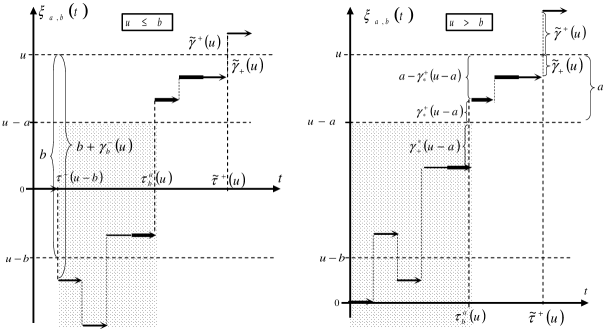
Figure 1: Modified Risk Process

By $\tilde{\tau}^{+}(u),\tilde{\gamma}_{+}(u)$, $\tilde{\gamma}^{+}(u)$ we denote the overjump functionals for the modified process $\xi_{a,b}(t)$ (see Figure 1). We also denote

$$\mathbf{f}^{a,b}_{s}(dx,dy/u)=\mathbf{E}\left[e^{-s\tilde{\tau}^{+}(u)},\tilde{\gamma}_{+}(u)\in dx,\tilde{\gamma}^{+}(u)\in dy,\tilde{\tau}^{+}(u)<\infty\right].$$

Then the Gerber–Shiu function can be defined as follows (see [9])

$$\boldsymbol{\Phi}^{a,b}_{s}(u)=\int_{0}^{\infty}\int_{0}^{\infty}w(x,y)\mathbf{f}^{a,b}_{s}(dx,dy/u),$$

where $w(x,y)$, $x,y>0$ is a nonnegative function (penalty). If the parameter $s$ is regarded as the force of interest, then $\boldsymbol{\Phi}^{a,b}_{s}(u)$ can be regarded as a discounted expected penalty at the time to ruin.

Assume that the process $e^{u-\xi_{a,b}(t)}$ describes the price of a stock whose variations have the form of random jumps. We now consider a perpetual American put option with strike price $K$. The payoff at time $t$ is equal to $(K-e^{u-\xi_{a,b}(t)})_{+}$. For the scalar case, the optimal strategy is as follows

$$\tau_{\beta}=\inf\{t>0:e^{u-\xi_{a,b}(t)}<e^{\beta}\},$$

where exercise boundary $\beta$: $e^{\beta}\leq\min(e^{u},K)$. Assume that the market is risk neutral. Then the price of an option is defined as the expected discounted payoff

$$\mathbf{E}\left[e^{-s\tau_{\beta}}(K-e^{u-\xi_{a,b}(\tau_{\beta})})_{+}\right]$$

or, in view of the fact that $\tau_{\beta}\dot{=}\tilde{\tau}^{+}(u-\beta)$, as follows

$$\mathbf{E}\left[e^{-s\tilde{\tau}^{+}(u-\beta)}(K-e^{\beta-\tilde{\gamma}^{+}(u-\beta)})_{+}\right].$$

Therefore, $\boldsymbol{\Phi}^{a,b}_{s}(u-\beta)$ with $w(x,y)=(K-e^{\beta-y})_{+}$ can also be regarded as the price of perpetual American put option  [10, p.12].

Theorem 2.

For the modified process$\{\xi_{a,b}(t),x(t)\}$

1) if $\,0<u\leq b$, then

$$\mathbf{f}^{a,b}_{s}(dx,dy/u)=\mathbf{f}^{+}_{b,s}(dx,dy/u)+\mathbf{B}_{b}(s,u)\int_{0}^{\infty}\mathbf{C}e^{-\mathbf{C}z}\mathbf{f}^{a,b}_{s}(dx,dy/z+b)dz;$$ (10)

2) if $\,b<u$, then

$$\mathbf{f}^{a,b}_{s}(dx,dy/u)=\mathbf{f}^{*}_{s}(dx-a,dy+a/u-a)I\{x>a\}+\\ +\int_{0}^{a}\mathbf{g}^{*}_{s}(dz/u-a)\biggl{(}\mathbf{f}^{+}_{b,s}(dx,dy/a-z)+\mathbf{B}_{b}(s,a-z)\int_{0}^{\infty}\mathbf{C}e^{-\mathbf{C}v}\mathbf{f}^{a,b}_{s}(dx,dy/v+b)dv\biggr{)},$$ (11)

where

$$\left(\!\mathbf{I}-\int_{0}^{\infty}\!\!\mathbf{C}e^{-\mathbf{C}z}\int_{0}^{a}\mathbf{g}^{*}_{s}(dv/b-a+z)\mathbf{B}_{b}(s,a-v)dz\!\right)\int_{0}^{\infty}\!\!\mathbf{C}e^{-\mathbf{C}z}\mathbf{f}^{a,b}_{s}(dx,dy/z+b)dz=\\ =\!\!\!\int_{0}^{\infty}\!\!\!\mathbf{C}e^{-\mathbf{C}z}\!\biggl{(}\!\mathbf{f}^{*}_{s}(dx-a,dy+a/b-a+z)I\{x>a\}+\!\int_{0}^{a}\!\!\mathbf{g}^{*}_{s}(dv/b-a+z)\mathbf{f}^{+}_{b,s}(dx,dy/a-v)\!\biggr{)}dz.$$ (12)

Proof.

Relation (10) is an analog of the result obtained in [6]. By using the formula of total probability and the strict Markov property, for $u>b$, we find

$$\mathbf{E}\left[e^{-s\tilde{\tau}^{+}(u)},\tilde{\gamma}_{+}(u)\in dx,\tilde{\gamma}^{+}(u)\in dy,\tilde{\tau}^{+}(u)<\infty\right]=\\ \quad=\mathbf{E}\biggl{[}e^{-s{\tau}_{*}^{+}(u-a)},{\gamma}^{*}_{+}(u-a)+a\in dx,{\gamma}_{*}^{+}(u-a)-a\in dy,\gamma_{*}^{+}(u-a)>a,{\tau}_{*}^{+}(u-a)<\infty\biggr{]}+\\ \quad\quad+\int_{0}^{a}\mathbf{E}\left[e^{-s{\tau}_{*}^{+}(u-a)},{\gamma}_{*}^{+}(u-a)\in dz,{\tau}_{*}^{+}(u-a)<\infty\right]\times\\ \times\mathbf{E}\left[e^{-s\tilde{\tau}^{+}(a-z)},\tilde{\gamma}_{+}(a-z)\in dx,\tilde{\gamma}^{+}(a-z)\in dy,\tilde{\tau}^{+}(a-z)<\infty\right].$$ (13)

This yields relation (11). Relation (12) is obtained from (11) as a result of the integral transform. ∎

In the scalar case $(m=1)$ the matrix relations become somewhat simpler. If we set $w(x,y)=1$, then ${\Phi}^{a,b}_{0}(u)$ is the ruin probability for the modified process.

Corollary 1.

For the scalar modified process $\xi_{a,b}(t)$

1) if $\,0<u\leq b$, then

$${\Phi}^{a,b}_{0}(u)=1-B_{b}(u)\left(1-\int_{0}^{a}g_{*}(dz/b-a+\theta^{\prime}_{c})B_{b}(a-z)\right)^{-1}P^{*}_{+}(b-a+\theta^{\prime}_{c});$$ (14)

2) if $\,b<u$ then

$${\Phi}^{a,b}_{0}(u)=P^{*}_{+}(u-a)-\int_{0}^{a}g_{*}(dz/u-a)B_{b}(a-z)\times\\ \times\left(1-\int_{0}^{a}g_{*}(dz/b-a+\theta^{\prime}_{c})B_{b}(a-z)\right)^{-1}P^{*}_{+}(b-a+\theta^{\prime}_{c}),$$ (15)

where

$$P^{*}_{+}(b-a+\theta^{\prime}_{c})=\int_{0}^{\infty}ce^{-cx}\mathrm{P}\{\xi^{+}_{*}<b-a+x\}dx,$$

$$g_{*}(dz/b-a+\theta^{\prime}_{c})=\int_{0}^{\infty}ce^{-cx}\mathrm{P}\{\gamma^{+}_{*}(b-a+x)\in dz,\text{ and }\tau^{+}_{*}(b-a+x)<\infty\}dx.$$

Example. Assume that, for the scalar risk process, the premiums $\xi^{\prime}_{n}$ have exponential distributions with parameter $\tilde{c}$, whereas the claims $\xi_{n}$ obey the Erlang distribution(2):

$$\mathrm{P}\{\xi_{n}<x\}=\delta^{2}xe^{-\delta x},x>0.$$

It is necessary to determine the corresponding ruin probability for $u\leq b$.

According to Example 5.2 [3], for $\mathrm{E}\xi(1)<0$ and $\mathrm{E}\xi_{*}(1)<0$ we find

$$\mathrm{P}\left\{\xi^{+}_{*}<u\right\}=P^{*}_{+}(u)=1-a^{*}_{1}e^{-r^{*}_{1}u}-a^{*}_{2}e^{-r^{*}_{2}u};$$

$$M^{*}_{+}(0+)=\frac{1}{\lambda},dM^{*}_{+}(x)=\frac{1}{c_{*}|\mathrm{E}\xi_{*}(1)|}dP^{*}_{+}(x),R^{-}(0)=p^{-}(0)=0,$$

$$B_{b}(u)=\left(1-a_{1}e^{-r_{1}u}-a_{2}e^{-r_{2}u}\right)\left(1-b_{1}e^{-r_{1}b}-b_{2}e^{-r_{2}b}\right)^{-1},$$

where the quantities $a_{i},a^{*}_{i}$, and $b_{i}$ are independent of $u$ and $b$; $r_{i}$ and $r^{*}_{i}$ are positive roots of the Lundberg equation for the processes $\xi(t)$ and $\xi_{*}(t)$, respectively. By using (5) and (14), we conclude (for $u\leq b$):

$$\mathrm{P}\left\{\tilde{\tau}^{+}(u)<\infty\right\}=1-\frac{(1-a_{1}e^{-r_{1}u}-a_{2}e^{-r_{2}u})(1-f^{*}_{1}e^{-r^{*}_{1}(b-a)}-f^{*}_{2}e^{-r^{*}_{2}(b-a)})}{P(u,a,b)},$$ (16)

$$P(u,a,b)=1-f_{2}e^{-r_{1}b}-f_{3}e^{-r_{2}b}+(g_{11}+g_{12}(b-a))e^{-\delta(b-a)}+\\ +(g_{21}+g_{22}(b-a))e^{-\delta(b-a)-r_{1}a}+(g_{31}+g_{32}(b-a))e^{-\delta(b-a)-r_{2}a},$$

where $f_{i},f^{*}_{i}$, and $g_{i,j}$ are independent of $u,a$ and $b$.

Assume that $c=1$, $c_{*}=4$, $\delta=20$, $\lambda_{1}=2$, and $\lambda_{2}=1$. Then $\mathrm{E}\xi(1)=-19/10$ and $\mathrm{E}\xi_{*}(1)=-2/5$. The corresponding Lundberg roots are $r_{1}=8$, $r_{2}=95/3$ and $r^{*}_{1}=20/3$, $r^{*}_{2}=32$.

In addition, the distribution of the absolute maximum of the process $\xi_{*}(t)$ and the probability of exit of the process $\xi(t)$ from the interval $(u-b,b)$ through the lower boundary are given by the formulas

$$\mathrm{P}\left\{\xi^{+}_{*}<u\right\}=1-\left(\frac{32}{57}e^{-20x/3}-\frac{9}{95}e^{-32x}\right);$$

$$B_{b}(u)=\mathrm{P}\left\{\xi(\tau(u,b))\leq u-b\right\}=\frac{1+\frac{49}{426}e^{-95u/3}-\frac{171}{355}e^{-8u}}{1+\frac{1}{284}e^{-95b/3}-\frac{19}{355}e^{-8b}}.$$

For $a=b$, by using (16), we arrive at the following expression for the ruin probability

$$\mathrm{P}\left\{\tilde{\tau}^{+}(u)<\infty\right\}=1-\frac{1+\frac{49}{426}e^{-95u/3}-\frac{171}{355}e^{-8u}}{1-\frac{45}{111328}e^{-95b/3}+\frac{19}{852}e^{-8b}}.$$

References

• [1] Karnaukh, E.V. Two-limit problems for almost semicontinuous processes defined on a Markov chain. (Ukrainian, English)//Ukr. Mat. Zh. 59, No. 4 (2007), 555-565, translation in Ukr. Math. J. 59, No. 4 (2007), 620-632, arXiv:0909.1420v1[math.PR].
• [2] Karnaukh, E.V. Overshoot functionals for almost semicontinuous processes defined on a Markov chain // Teor. Imovir. ta Matem. Statyst., No.76 (2007), 45-52, translation in Theor. Probability and Math. Statist. No. 76 (2008), 49-57, arXiv:0909.3690v1[mathPR].
• [3] Gusak D.V., Boundary value problems for processes with independent increments in the risk theory[in Ukrainian], Institute of Mathematics, Ukrainian National Academy of Sciences, Kyiv, 2007.
• [4] Asmussen S., Ruin Probabilities, World Scientific, Singapore, 2000.
• [5] Jasiulewicz H., Probability of ruin with variable premium rate in a Markovian environment, Insurance: Mathematics and Economics 29 (2001), 291–296.
• [6] Bratiychuk M.S., Derfla D., On a modification of the classical risk process, Insurance: Mathematics and Economics 41 (2007), 156–162.
• [7] Rolsky T., Shmidly H., Shmidt V., Teugels J., Stochastic Processes for Insurance and Finance, Wiley, New York, 1999.
• [8] Gusak D.V., Boundary problems for processes with independent increments on Markov chains and for semi-Markov processes, Institute of Mathematics, Ukrainian National Academy of Sciences, Kyiv, 1998.
• [9] Gerber H.U., Shiu S.W., On the time value of ruin, North American Actuarial Journal 2 (1998), N 1, 48–78.
• [10] Gerber H.U., Shiu S.W., From ruin theory to pricing reset guarantees and perpetual put optoins, Insurance: Mathematics and Economics 24 (1999), 3–14.