Uncovering Evolutionary Ages of Nodes in Complex Networks

Abstract

In a complex network, different groups of nodes may have existed for different amounts of time. To detect the evolutionary history of a network is of great importance. We present a spectral-analysis based method to address this fundamental question in network science. In particular, we find that there are complex networks in the real-world for which there is a positive correlation between the eigenvalue magnitude and node age. In situations where the network topology is unknown but short time series measured from nodes are available, we suggest to uncover the network topology at the present (or any given time of interest) by using compressive sensing and then perform the spectral analysis. Knowledge of ages of various groups of nodes can provide significant insights into the evolutionary process underpinning the network. It should be noted, however, that at the present the applicability of our method is limited to the networks for which information about the node age has been encoded gradually in the eigen-properties through evolution.

1 Introduction

Many large, complex networks in existence today are the results of some evolutionary processes such as growth Newman:book . The Internet is one best example, which has undergone tremendous expansion in the past two decades. Growth in a decentralized manner also appears to be the hallmark of other types of networks such as various biological, social and economical networks (e.g., Facebook). Given a complex network but without any knowledge of its evolutionary history, one might be interested in the distribution of the “ages” of various nodes or subgroups of nodes in the network. Information about the node ages can provide deep insights into the organization and structure of the underlying network, and may have significant applications. For example, in a social network, the lifetimes of certain subgroups of nodes may be closely related to the network backbone structure in terms of the roles that these subgroups play in the function of the network, e.g., leadership roles. In a biological network, nodes of longer lifetimes can be more critical to the various functions of the network. It is thus of considerable interest to develop a systematic method to uncover the evolutionary ages of subgroups of nodes in complex networks.

Two situations arise when addressing the age-detection problem in complex networks: (1) network topology is known and (2) the topology is unknown but only time series measured or observed from various nodes are available. In the first case we shall establish that the spectrum of the network connectivity matrix, or the Laplacian matrix, is directly related to the evolutionary ages of various subgroups of nodes in the network. In the second case, we make use of a recently developed method of time-series based reverse engineering of complex networks WYLHK:2011 to uncover the network topology, and then could analyze the spectrum of the predicted Laplacian matrix to obtain estimates of the age distribution of nodes. Our approach thus defines a framework in which the problem of evolutionary-age detection of nodes in complex networks can be addressed in systematic way. While our method does not require a positive correlation between the node degree and age, a correlation between the eigenvalue and the node age is necessary.

It is useful to point out that for the class of scale-free networks that are generated according to the preferential-attachment rule BA:1999 , the problem of evolutionary-age estimation may be trivial. In particular, this growth rule stipulates that the probability for an existing node to acquire new links is proportional to its degree, implying a strong correlation between the node degree and its lifetime. Thus, for a scale-free network evolved predominantly according to the preferential-attachment rule, the ages of various nodes can be predicted simply by examining the degrees. However, many real-world networks deviate significantly from the scale-free topology Newman:book and, for them the problem of detecting node evolutionary ages is nontrivial. Nonetheless, scale-free networks provide an ideal testbed to validate our spectrum-analysis method.

We emphasize that, although our method is suitable even for networks for which there is no positive correlation between node degree and age, its applicability is limited to networks for which there is a positive correlation between the properties of the eigenmodes and the node age. For networks with which no evolutionary process can be affiliated, such as various citation networks and twitter-type of social networks where the importance of a node may not be related with its age, our method is not applicable.

In Sec. 2, we describe the main idea underlying our method. In Sec. 3, we validate the method by using scale-free networks generated by the standard preferential-attachment rule and by the duplication/divergence mechanism, which are especially relevant to social and biological systems, respectively. In Sec. 4, we consider a realistic biological network, the protein-protein interaction network for which the age distribution of nodes is available, to further validate our method. In Sec. 5, we address the situation where the network topology is not known a priori but only time series are available, make use of the reverse-engineering approach WYLHK:2011 to map out the network topology, and demonstrate that the approach yields correctly and accurately the spectrum of the Laplacian matrix. A brief conclusion is presented in Sec. 6.

2 Method

For a complex network of $N$ nodes, its topological structure can be described by the Laplacian matrix $L$ ZHU:2008 ; YANG:2006 ; REN:2009 ; REN:2010 ; SARIKA:2011 , where the off-diagonal elements of $L$ are $L_{i\neq j}=L_{j\neq i}=1(0)$ if the nodes $i$ and $j$ are connected (disconnected), respectively. The diagonal elements are $L_{ii}=-\sum_{j\neq i}L_{ij}=-k_{i}$, where $k_{i}$ is the number of the nodes connected directly with the node $i$ (node degree). The eigenvalues of $L$ are nonnegative and can be ranked as $0=\lambda_{1}\leq\lambda_{2}\cdots\leq\lambda_{N}$. The corresponding eigenvectors are $X_{1},X_{2},\cdots,X_{N}$, whose wavelengths are sorted in a descending order. Each eigenvector contains components concentrated on various nodes in the network.

For a regular or a small-world network WS:1998 , the eigenvectors typically exhibit some wave patterns with certain wavelengths ROH:2004 ; PHL:2007 . When a perturbation is applied to the network, the affected eigenvectors are those whose wavelengths match the size of the perturbation (i.e., the number of nodes that it affects). In this case, some localized structure in the affected eigenvectors can emerge. Eigenvectors associated with small eigenvalues usually have large wavelengths, and so they are sensitive to perturbation on a global scale. In contrast, eigenvectors associated with large eigenvalues are most sensitive to localized perturbations that are applied to a small set of nodes in the network. The responses of the eigenvectors to perturbations thus reflect the structure of the network at different scales. An example is given in Fig. 1 for a one-dimensional regular lattice of $N=100$ nodes with periodic boundary condition, where each node is connected with 2 neighbors on either side so that the node has 4 nearest neighbors. Shown in Fig. 1(a) are representative eigenvectors, where the values of $N\cdot X_{i}^{2}(s)$ are plotted and $X_{i}^{2}(s)$ is the $s$th component of the eigenvector $X_{i}$. We see that the eigenvectors represent periodic waves of wavelengths ranging from $N$ to $2$. To observe the effect of local structural perturbation on the eigenvectors, we add two more links to each node in the group of nodes whose indices are between 40 and 60 so that each node in this perturbed group now has six nearest neighbors. Let $\lambda^{\prime}_{i}$ ($i=1,\ldots,N$) be the eigenvalues in the perturbed network. Figure 1(b) shows some representative eigenvectors. We observe that the eigenvectors associated with small eigenvalues, e.g., $\lambda^{\prime}_{1}$, $\lambda^{\prime}_{20}$, $\lambda^{\prime}_{40}$, $\lambda^{\prime}_{60}$, and $\lambda^{\prime}_{80}$, are basically unchanged. However, eigenvectors associated with relatively large eigenvalues, such as $\lambda^{\prime}_{100}$, are strongly altered by the perturbation but the changes are focused on the perturbed group of nodes. Figure 1(c) shows the distribution of the magnitudes of all eigenvectors on nodes in the network, where we see that those associated with eigenvalues $\lambda^{\prime}_{90}$ to $\lambda^{\prime}_{100}$ are sensitive to the perturbation with large variations appearing on the perturbed nodes.

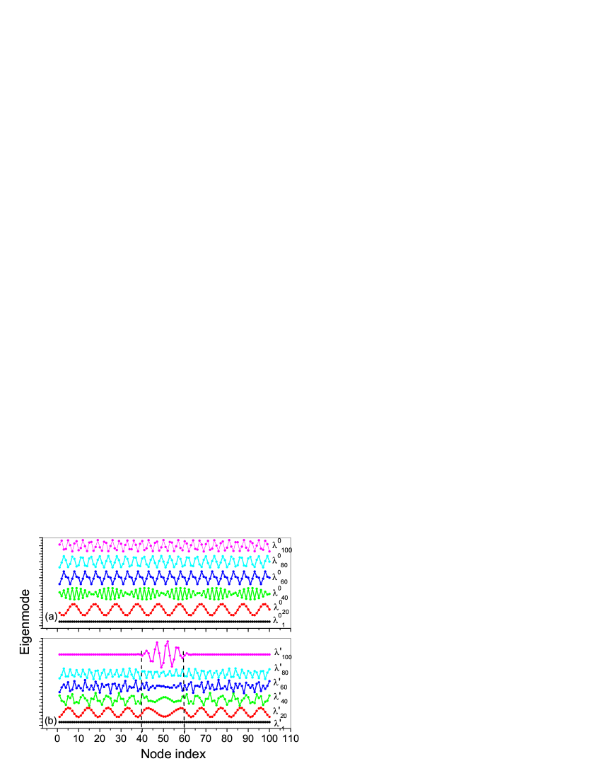
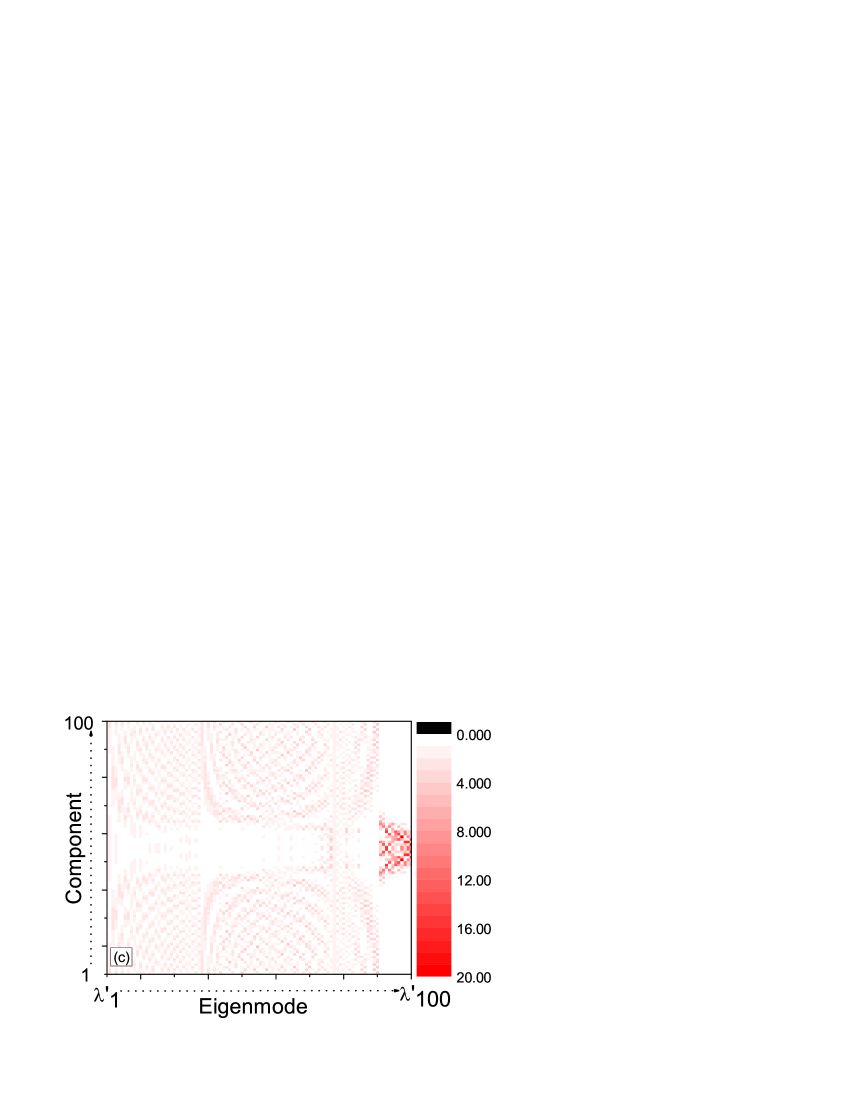
Figure 1: (color online.) For a regular ring network of 100 nodes where each node has four neighbors, (a) examples of typical, periodic-wave like eigenvectors, (b) typical eigenvectors when each node in the group of indices between 40 and 60 acquires two additional links, one on each side. We observe significant distortions from the periodic-wave pattern, which are localized between the 40th and 60th components of eigenvectors associated with relatively large eigenvalues. (c) Representation of all eigenvectors, where those associated with eigenvalues from $\lambda^{\prime}_{90}$ to $\lambda^{\prime}_{100}$ are significantly more sensitive to the structural perturbation to the network.

For complex networks that do not possess a regular backbone, such as random ER:1960 and scale-free BA:1999 networks, the eigenvectors in general do not exhibit any periodic wave structure. Nonetheless, the observation that the eigenvectors associated with larger eigenvalues are more sensitive to structural perturbations can be used to infer the evolutionary age of nodes. To see this, consider a scale-free network evolved according to the preferential-attachment rule BA:1999 , for which there is a positive correlation between the node degree and lifetime. That is, nodes of “old” ages tend to have more links and they are thus more susceptible to perturbations applied randomly to the network during the evolutionary process. Since the eigenvectors of large eigenvalues are quite sensitive to perturbations (c.f., Fig. 1), we expect the large-degree nodes to dominate these eigenvectors. As a result, large eigenvalues tend to correspond to nodes of long lifetime. This argument suggests that, nodes having the most significant components of the eigenvectors associated with the largest eigenvalues are likely to possess the longest lifetime in the network.

3 Validation using scale-free networks

To exemplify the relation between eigenvalues and node ages, we consider standard scale-free networks BA:1999 . Each network has $N=2000$ nodes, which is evolved following the preferential-attachment rule so that the age of the $i$th node is $N-i+1$. For a given eigenvalue, the lifetime of the associated eigenvector is the average age of all nodes contained in the vector, weighted by the respective components of the eigenvector. Figures 2(a-c) show the ages of the eigenvectors $X_{i}$ versus the index $i$ for three networks of different edge density $w$. The significant feature common to all three cases is that the average age of the nodes dominating some eigenvector increases on average with the eigenvalue. The average degree of each eigenvector, i.e., the weighted average of the degrees of all nodes associated with the vector, shows the same tendency, as shown in Figs. 2(d-f), where the average degree is presented on a logarithmic scale. For each network, the sizes of the eigenvectors are shown in Figs. 2(g-i), where the size of an eigenvector is defined to be the number of nodes on which the vector component is larger than a small threshold value. For sufficiently dense network, e.g., Fig. 2(i), the size tends to decrease on average with the eigenvalue, indicating that a small group of nodes have extraordinarily long lifetimes in the network and their relative ages can be identified simply by examining the associated eigenvalues. Figures 2(j-l) show, for $W=2,4$ and $8$, respectively, the average evolution age versus the node degree. We observe an approximately monotonic relation for small degree. However, when the node degree is larger than 10, the relation deteriorates quickly and the relations approach a constant.

To further demonstrate our method, we have analyzed a scale-free cellular network generated by mechanism different than that of the preferential-attachment rule, namely the protein-protein interaction(PPI) networks. In such a network, duplication and divergence are believed to be responsible for the topological structure PPIB:2003 . We start from a small, connected graph as a seed and duplicate a randomly selected existing protein at each step. The new comer duplicates exactly the connection pattern of its generator in the network. Due to mutations, some of the duplicated edges are broken with probability $p$, while new edges are generated with probability $q$ between the new comer and other existing nodes. To compare with the PPI network of the Baker’s Yeast (to be described in the next Section), we generate networks with comparable parameters. In particular, a typical network has $2235$ nodes and average degree of $10.52$, and degree distribution follows power-law with exponent $2.3$. In a wide range of eigenvalues there exists a strong correlation between the eigenvalue and average age, as shown in Fig.3(a). We observe that, the curve of average age versus degree exhibits large fluctuations, as shown in Fig.3(d). It is thus not possible to obtain information about node age from degree. However, behaviors of the eigenmodes can reveal the age information, as will be demonstrated in Sec. 4.

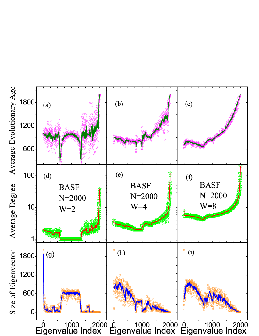
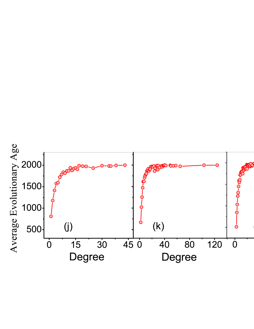
Figure 2: (Color online.) For three scale-free networks generated according to the standard preferential-attachment rule with edge density $w=2,4,8$ (corresponding to the left, middle, and right column, respectively), (a-c) average ages, (d-f) average degree (on a logarithmic scale), and (g-i) size of eigenvector versus the eigenvalue index $i$. Eigenvectors associated with large eigenvalues generally have small sizes, but their ages are “older” in the network. (j-l) Average age versus degree. We see that, while small degree is related with the average age, information about node age deteriorates quickly as the degree is increased.

4 Evolution ages of nodes in a protein-protein interaction network

To lend more credence to our proposition that the evolutionary ages of nodes can be inferred from the eigenvalues, we now consider a class of networks in systems biology, protein-protein interaction (PPI) networks. These networks are the result of a number of evolutionary mechanisms such as duplications of genes and reattachments of links between the proteins. Specifically, we analyze the PPI network of the baker’s yeast (Saccharomyces cerevisiae) wangner01 ; wangner03 . Von Mering et al. mering02 analyzed a total of 80000 interactions among 5400 yeast proteins reported previously and assigned each interaction a confidence value. In order to reduce the effect of false positives, we focus on 11855 interactions with high and medium confidence values among 2617 yeast proteins. In a PPI network, each protein is a node and each pairwise interaction represents a link between two nodes. Since our goal is to assess, through the eigenvalues, the evolutionary ages of the nodes, we neglect the directions of the edges. The largest connected component of the PPI network contains 2235 nodes. In systems biology, the evolutionary processes of the proteins are classified into four iso-temporal groups woese87 : prokaryotes, eukarya, fungi, and yeast, to which numbers $4,3,2$ and $1$ are assigned according to their evolutionary process from ancient to modern times, respectively. The evolutionary age of a protein is the largest number from the groups it presents. For example, the protein YHR$037$w occurs in the groups prokaryotes($4$), eukarya($3$), fungi($2$), which means that it can be found from the ancient prokaryotes, so that its age is $4$. Figure 4(a) shows the average evolutionary age of nodes in eigenvector versus the eigenvalue index, which is similar to the behavior in Figs. 2(a-c). This suggests that for a realistic biological network, there is indeed a positive correlation between the eigenvalues of the Laplacian matrix and the evolutionary ages of groups of nodes. Since PPIs typically possess a scale-free structure RSMOB:2002 , we expect the average degree of groups of nodes to exhibit similar behaviors as in Figs. 2(d-f). This is indeed the case, as shown in Fig. 4(b). The sizes of various eigenvectors are shown in Fig. 4(c). Again the behavior is similar to those in Figs. 2(g-i). From Fig. 4(d), relation of average age versus degree, we see that the degree contains no information about the node age.

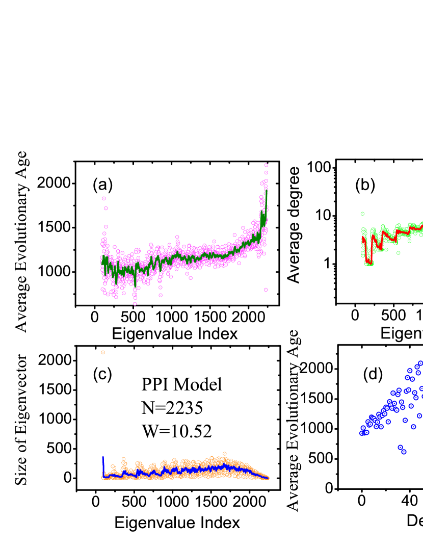
Figure 3: (Color online.) For scale-free networks generated by duplication/divergence-based mechanism from PPI network of the Baker’s Yeast, (a) average age versus eigenvalue index, (b) average degree versus eigenvalue index, and (c) size of eigenvector versus the eigenvalue index. Eigenvectors associated with large eigenvalues generally have small sizes, but their ages are “older” in the network. (d) Average age versus degree. Because of large fluctuation, the degree cannot give age-related information, but the eigenvalues can.

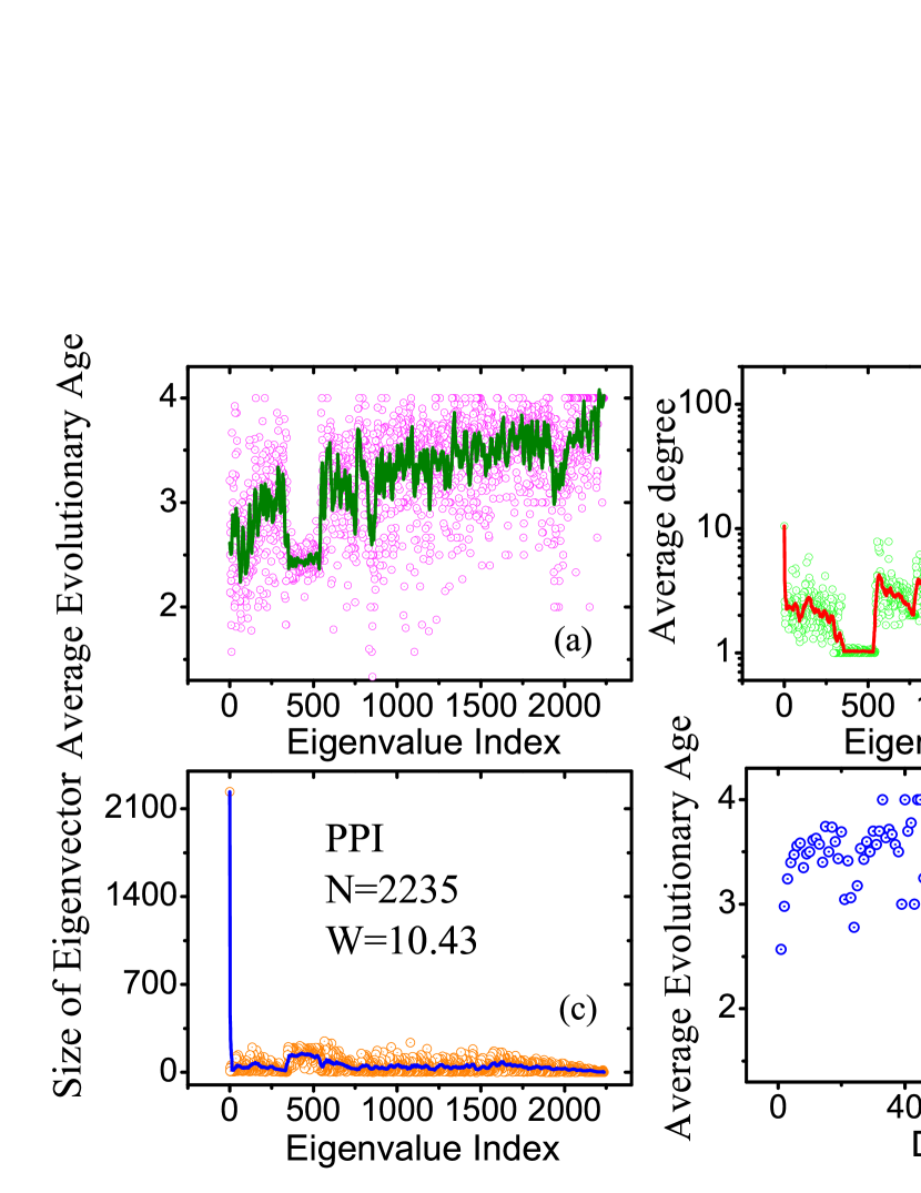
Figure 4: (Color online.) For the largest connected component of the PPI network of the baker’s yeast with 2235 nodes, (a) the evolutionary age, (b) average degree (on a logarithmic scale), and (c) size of eigenvector versus the eigenvalue index $i$. These results further indicate that the evolutionary ages of various nodes in the network can be inferred from the eigenvalue spectrum of the Laplacian matrix. (d) Average age versus degree. We see that degree does not reveal age-related information.

5 Time-series based detection of evolutionary ages of nodes

We now address the situation where the network topology is unknown but only time series measured or observed from various nodes are available. We shall apply a recently developed approach WYLHK:2011 based on compressive sensing CRT:2006 ; C:2006 ; D:2006 ; B:2007 ; C:2008 ; CR:2005 to uncover the complex-network topology and then could analyze the spectrum of the predicted Laplacian matrix to estimate the evolutionary ages of nodes. The unique feature of compressive sensing lies in its extremely low data requirement: very little observation is needed to obtain a target sparse signal. In general, the problem of compressive sensing can be described as to reconstruct a sparse vector $\mathbf{a}\in R^{N}$ from linear measurements $\mathbf{X}$ about $\mathbf{a}$ in the form: $\mathbf{X}=\mathbf{G}\cdot\mathbf{a}$, where $\mathbf{X}\in R^{M}$ and $\mathbf{G}$ is an $M\times N$ matrix. Accurate reconstruction can be achieved by solving the following convex optimization problem CRT:2006

$$\min\|\mathbf{a}\|_{1}\quad\mbox{subject \ to}\quad\mathbf{G}\cdot\mathbf{a}=\mathbf{X},$$ (1)

where $\|\mathbf{a}\|_{1}=\sum_{i=1}^{N}|\mathbf{a}_{i}|$ is the $L_{1}$ norm of vector $\mathbf{a}$ and $M\ll N$, $i.e.,$, the number of measurements can be much less than the number of components of the unknown signal. Various solutions of the convex optimization problem (1) have been worked out in the applied-mathematics literature CRT:2006 ; C:2006 ; D:2006 ; B:2007 ; C:2008 ; CR:2005 .

To uncover network topology based on data, it is necessary to cast the problem in the form (1). The basic hypothesis is that a complex networked system can be viewed as a large dynamical system that generates oscillatory time series at various nodes. Under this hypothesis, it is straightforward to formulate the problem under the compressive-sensing paradigm, details of which can be found in Ref. WYLHK:2011 .

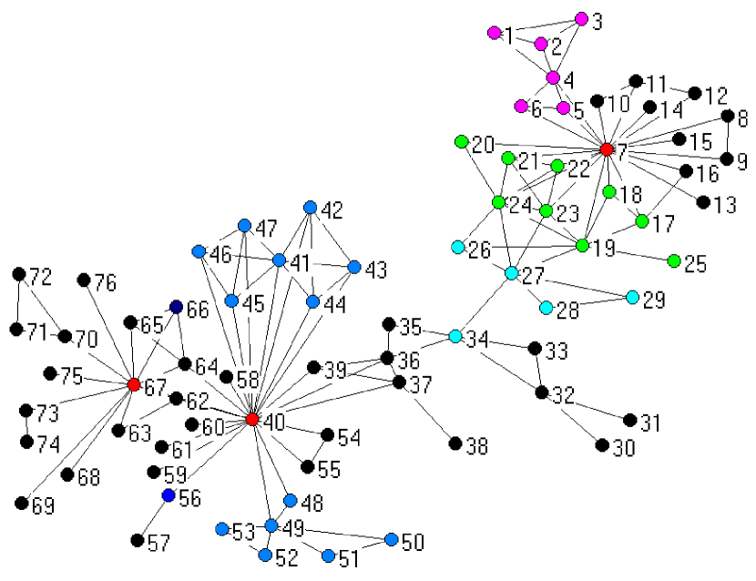
Figure 5: (Color online.) Schematic illustration of the largest component of the SFI collaboration network and the clustered structure revealed by an eigenvalue/eigenvector analysis.

To give a concrete example, we consider a real-world network, the Santa Fe Institute (SFI) collaboration network girvan02 . There are $N=76$ nodes in the largest connected component of the network and the average degree is about 3. A schematic illustration of the network is shown in Fig. 5. A spectral analysis reveals that the eigenvectors associated with $\lambda_{76}$, $\lambda_{75}$ and $\lambda_{74}$ characterize the three hubs: 40, 7 and 67, all marked by red. The eigenvector associated with $\lambda_{73}$ involves a group of nodes numbered between 17 and 25 (marked by green). For $\lambda_{72}$, the corresponding eigenvector covers nodes 26 to 29, and node 34 (marked by cyan). The three clusters: nodes 41 to 47 (blue), 1 to 6 (magenta), and 48 to 53 (violet), are represented by eigenvectors $\lambda_{70}$, $\lambda_{69}$, and $\lambda_{68}$, respectively. In fact, clusters of larger scales can be identified for smaller eigenvalues.

Now assume that the network topology is unknown but an oscillatory time series from each node is available. To simulate the situation, we assume that the dynamics of each node is described by the chaotic Rössler oscillator Rossler:1976 . Applying the compressive-sensing based method to uncover the network topology, we can then perform a spectral analysis to estimate the ages of various nodes in the network. Figure 6 shows the eigenvalues of the predicted and the actual Laplacian matrix. We observe an excellent agreement.

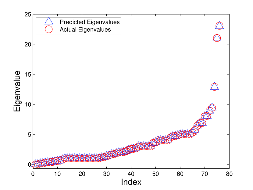
Figure 6: (Color online) Sorted eigenvalues of the predicted and actual Laplacian matrix of the SFI collaboration network. The number of data points used in uncovering the network structure is about $40\%$ of the number of total unknown coefficients in the power-series expansion.

6 Conclusions

In summary, we have developed a procedure to estimate the evolutionary ages of nodes in complex networks. The basic observation is that eigenvectors associated with different eigenvalues of the Laplacian matrix can typically represent highly localized groups of nodes in the network. A qualitative argument can then be made for the existence of positive correlation between the node ages and the magnitudes of the eigenvalues. This means that, when the network topology is known, a simple eigenvalue analysis can lead to reliable information about the age distribution of nodes in the network. For situations where the network topology is unknown but time series from nodes are available, it is necessary to uncover the topology in order to estimate the node ages, and we have demonstrated that this can be done efficiently using compressive sensing. Examples from model and real-world networks, including a PPI network, are used to validate our approach. We hope our method to find applications in fields such as systems biology,the propagation of a rumor, a fashion, a joke, or a flu, where estimating node ages can be of significant value.

The network-reconstruction technique used in our work is based on compressive sensing, which works for situations where the types of mathematical forms of the nodal dynamical systems and coupling functions are known (although details of these functions are not required) and can be represented by series expansion. So far the method has not been applied to gene-regulatory networks due to difficulty to find suitable series expansions. The recent method by Hempel et al. HKKN:2011 is based on extracting statistical information and has been demonstrated to work well for gene-regulatory networks.

While many real-world systems such as gene regulatory and supply chain networks are directed, our present work focused on undirected networks. The main consideration is that many networks generated by some kind of evolutionary processes or constructed through experiments tend to undirected. For example, the Baker Yeast obtained through the approach of prey and predator contains no information about the directionality of the nodal interactions. Our method is based on the observation that local structures, e.g., densely connected clusters, can induce large components in the eigenvectors. Hubs or clusters of hubs can then be detected by the eigenvectors corresponding to largest eigenvalues, while clusters of larger sizes can be uncovered by eigenvectors of smaller eigenvalues. Different eigenmodes can be used to detect clusters of varying scales, providing a correlation with the evolutionary ages in situations where hubs or clusters of hubs are formed by history. The principle on which our method is based thus does not take into account directionality in the node-to-node interactions. To develop a method to uncover the evolutionary ages for directed complex networks remains to be an interesting but open question at the present.

References

- (1) M. J. Newman, Networks: An Introduction (Oxford University Press, New York, 2010).
- (2) W.-X. Wang, R. Yang, Y.-C. Lai, V. Kovanis, and M. A. F. Harrison, Europhys. Lett. 94, 48006 (2011); W.-X. Wang, R. Yang, Y.-C. Lai, V. Kovanis, and C. Grebogi, Phys. Rev. Lett. 106, 154101 (2011).
- (3) A.-L. Barabási, and R. Albert, Science 286, 509 (1999).
- (4) G. M. Zhu, H. J. Yang, C. Y. Yin, B. Li, Phys. Rev. E 77, 066113 (2008).
- (5) H. J. Yang, F. C. Zhao, and B. H. Wang, Chaos 16 (2006).
- (6) J. Ren, and B. Li, Phys. Rev. E 79, 051922 (2009).
- (7) J. Ren, W. W. Wang, B. Li, and Y. C. Lai, Phys. Rev. Lett. 104, 058701 (2010).
- (8) S. Jalan, G. M. Zhu, and B. Li, Phys. Rev. E 84, 046107 (2011).
- (9) D. J. Watts and S. H. Strogatz, Nature (London) 393, 440 (1998).
- (10) J. G. Restrepo, E. Ott, and B. R. Hunt, Phys. Rev. Lett. 93, 114101 (2004).
- (11) K. Park, L. Huang, and Y.-C. Lai, Phys. Rev. E 75, 026211 (2007).
- (12) P. Erdös and A. Rényi, Publ. Math. Inst. Hung. Acad. Sci. 5, 17 (1960).
- (13) A. V. Vazquez, A. Flammini, A. Maritan, A. Vespignani, Complexus 1, 38 (2003).
- (14) A. Wagner, Mol. Biol. Evol. 18, 1283 (2001).
- (15) A. Wagner, Proc. R. Soc. Lond. Ser. B-Biol. Sci. 270, 457 (2003).
- (16) C. von Mering, R. Krause, B. Snel, M. Cornell, S. G. Oliver, S. Fields, and P. Bork, Nature 417, 399 (2002).
- (17) C. R. Woese, Microbiol. Rev. 51, 221 (1987).
- (18) E. Ravasz, A. L. Somera, D. A. Mongru, Z. Oltvai, and A.-L. Barabási, Science 297, 1551 (2002).
- (19) E. Candès, J. Romberg, and T. Tao, IEEE Trans. Inf. Theory 52, 489 (2006); Commun. Pure Appl. Math. 59, 1207 (2006).
- (20) E. Candès, in Proceedings of the International Congress of Mathematicians, Madrid, Spain, 2006.
- (21) D. Donoho, IEEE Trans. Inf. Theory 52, 1289 (2006).
- (22) R.G. Baraniuk, IEEE Signal Processing Mag. 24, 118 (2007).
- (23) E. Candès and M. Wakin, IEEE Signal Processing Mag. 25, 21 (2008).
- (24) E. Candès, and J. Romberg, http://www. acm. caltech.edu/l1magic, 2005.
- (25) M. Girvan, and M. E. J. Newman, Proc. Natl. Acad. Sci. U. S. A. 99, 7821 (2002).
- (26) O. E. Rössler, Phys. Lett. A 57, 397 (1976).
- (27) S. Hempel, A. Koseska, J. Kurths, and Z. Nikoloski, Phys. Rev. Lett. 107, 054101 (2011).