Assessing the redshift evolution of massive black holes and their hosts

Abstract

Motivated by recent observational results that focus on high redshift black holes, we explore the effect of scatter and observational biases on the ability to recover the intrinsic properties of the black hole population at high redshift. We find that scatter and selection biases can hide the intrinsic correlations between black holes and their hosts, with ‘observable’ subsamples of the whole population suggesting, on average, positive evolution even when the underlying population is characterized by no- or negative evolution. We create theoretical mass functions of black holes convolving the mass function of dark matter halos with standard relationships linking black holes with their hosts. Under these assumptions, we find that the local $M_{\rm BH}-\sigma$ correlation is unable to fit the $z=6$ black hole mass function proposed by Willott et al. (2010), overestimating the number density of all but the most massive black holes. Positive evolution or including scatter in the $M_{\rm BH}-\sigma$ correlation makes the discrepancy worse, as it further increases the number density of observable black holes. We notice that if the $M_{\rm BH}-\sigma$ correlation at $z=6$ is steeper than today, then the mass function becomes shallower. This helps reproducing the mass function of $z=6$ black holes proposed by Willott et al. (2010). Alternatively, it is possible that very few halos (of order 1/1000) host an active massive black hole at $z=6$, or that most AGN are obscured, hindering their detection in optical surveys. Current measurements of the high redshift black hole mass function might be underestimating the density of low mass black holes if the active fraction or luminosity are a function of host or black hole mass. Finally, we discuss physical scenarios that can possibly lead to a steeper $M_{\rm BH}-\sigma$ relation at high redshift.

1 Introduction

The constraints on black hole masses at the highest redshifts currently probed, $z\simeq 6$, are few, and seem to provide conflicting results. (i) There seems to be little or no correlation between black hole mass and velocity dispersion, $\sigma$ (Wang et al., 2010) in the brightest radio-selected quasars, (ii) typically black holes are ‘over-massive’ at fixed galaxy mass/velocity dispersion compared to their $z=0$ counterparts (e.g., Walter et al. 2004; at lower redshift see also McLure & Dunlop, 2004; Shields et al., 2006; Peng et al., 2006; Decarli et al., 2010; Merloni, 2010; Woo et al., 2008), but (iii) analysis of the black hole mass/luminosity function and clustering suggests that either many massive galaxies do not have black holes, or these black holes are less massive than expected (Willott et al., 2010, W10 hereafter).

As a result of point (ii), most authors propose that there is positive evolution in the $M_{\rm BH}-$galaxy relationships, and quantify it as a change in normalization, in the sense that at fixed galaxy properties (e.g. velocity dispersion, stellar mass), black holes at high redshift are more massive than today. For instance, Merloni et al. (2010) propose that $M_{\rm BH}-M_{*}$ evolves with redshift as $(1+z)^{0.68}$ while Decarli et al. (2010) suggest $(1+z)^{0.28}$. Point (iii) above, however, is inconsistent with this suggestion unless only about $1/100$ of galaxies with stellar mass $\simeq 10^{10}-10^{11}$ $M_{\odot}$ at $z=6$ host a black hole (W10). These galaxies are nonetheless presumed to be the progenitors of today’s massive ellipticals, which typically host central massive black holes.

When inferences on the population of massive black holes at the highest redshift are made, we have to take into consideration two important selection effects (see Lauer et al. 2007b). First, only the most massive black holes, powering the most luminous quasars, can be picked up at such high redshifts (Shen et al., 2008; Vestergaard et al., 2008). Second, as a result of the limited survey area of current imaging campaigns, only black holes that reside in relatively common galaxies can be recovered. Taken together, these biases imply that the observable population of black holes at high redshift will span a narrow range of masses and host properties (see also Adelberger et al. 2005, Fine et al. 2006).

In this paper, we explore the impact of these observational biases on attempts to recover the intrinsic properties of the black hole population. Our calculations are based on simple models grounded on empirical relations measured at much lower redshift, and therefore our results should be treated with caution. The aim of this paper is only to highlight the effects of the different factors that can influence the measurement of the intrinsic properties of the black hole population at high redshift.

In section 2 we describe how we generate Monte Carlo realizations of the $M_{\rm BH}-\sigma$ relation at $z=6$ varying the slope and normalization. We then select ‘observable’ systems from these samples, considering both ‘shallow’ or ‘pencil beam’ surveys, and test how well we can recover the parameters of the $M_{\rm BH}-\sigma$ relation from the ‘observable’ systems. In section 3 we discuss theoretical mass functions of black holes derived from the mass function of dark matter halos and various assumptions for the $M_{\rm BH}-\sigma$ relationship. Using these results, we test what assumptions can reproduce the black hole mass function derived by W10. We also discuss (section 4) why obtaining constraints on the average accretion rates and active fraction of black holes as a function of host mass is crucial to our understanding of the high-redshift massive black hole population. Finally, in section 5 we propose a simple theoretical framework that leads to selective accretion onto black holes in a manner that reconciles the observational results (i)-(ii) and (iii) above.

2 Scatter and evolution of the $M_{\rm BH}-\sigma$ relation at high redshift

We can qualitatively show the effects of selection biases with a simple exercise. Let us assume an evolution of the $M_{\rm BH}-\sigma$ relationship of the form:

$$M_{\rm BH,\sigma}=10^{8}\,{\rm M_{\odot}}\left(\frac{\sigma}{200\,{\rm km\,s^{-1}}}\right)^{\alpha}(1+z)^{\gamma},$$ (1)

where $\alpha$ is a function of redshift. Let us now also assume that at fixed $\sigma$ the logarithmic scatter in black hole mass is $\Delta=$0.25-0.5 dex ($M_{\rm BH}=M_{\rm BH,\sigma}\times 10^{\Delta\delta}$, where $\delta$ is normally distributed, see, e.g., Gultekin et al. 2009, Merloni et al. 2010. The results are qualitatively unchanged for a uniform distribution in $\log\Delta$.)

We create a Monte Carlo simulation of the $M_{\rm BH}-\sigma$ relation at $z=6$ assuming different values of $\alpha$ and $\gamma$. For this exercise we run a number of realizations $N(M_{h})\propto 1/n(M_{h})$, where $n$ is the number density of halos of a given mass ($M_{h}$) calculated through the Press & Schechter formalism. We then select only systems that are likely to be observed. We consider a shallow survey and a pencil beam survey. A wide, shallow survey would preferentially select systems with high luminosity, but has the advantage of a large area. For instance the SDSS quasar catalogue selects sources with luminosities larger than $M_{i}=-22.0$ ($\simeq 10^{45}$ erg s^-1) over an area of 9380 deg², corresponding to a volume of almost 7 comoving Gpc³ at z=6. To simulate a shallow survey, we select black holes with a sizeable mass, implying that large luminosities can be achieved, $M_{\rm BH}>3\times 10^{8}$ $M_{\odot}$  (see, e.g. Salviander et al. 2007; Lauer et al. 2007b, Vestergaard et al. 2008, Shen et al. 2008, 2010 for a discussion of this bias), and hosted in halos with space density $n>1$ Gpc^-3. Pencil beam surveys can probe fainter systems, but at the cost of a smaller area, e.g. the 2 Ms Chandra Deep Fields cover a combined volume of $\simeq 10^{5}$ comoving Mpc³ at $z=6$ and reach flux limits of $\simeq 10^{-17}$ and $\simeq 10^{-16}$ erg cm^-2 s^-1 in the 0.5-2.0 and 2-8 keV bands, respectively (the flux limit corresponds to a luminosity $\simeq 10^{43}$ and $\simeq 10^{44}$ erg s^-1at $z=6$). As an example of a pencil beam survey, we select black holes with mass $M_{\rm BH}>10^{7}$ $M_{\odot}$  hosted in halos with density $n>10^{3}$ Gpc^-3

To select sources that are observable in current surveys, we link the velocity dispersion, $\sigma$, to the mass of the host dark matter halo. Empirical correlations have been found between the central stellar velocity dispersion and the asymptotic circular velocity ($V_{\rm c}$) of galaxies (Ferrarese 2002; Baes et al. 2003; Pizzella et al. 2005). Some of these relationships (Ferrarese, Baes) mimic closely the simple $\sigma=V_{c}/\sqrt[]{3}$ definition that one derives assuming complete orbital isotropy. Indeed, it is difficult to imagine that the ratio between $\sigma$ and $V_{c}$ for massive, stable systems evolves strongly with redshift and that it can be much different from  $\sqrt[]{3}$ or $\sqrt[]{2}$ (see Binney & Tremaine 2008). Since the asymptotic circular velocity ($V_{\rm c}$) of galaxies is a measure of the total mass of the dark matter halo of the host galaxies, we can derive relationships between black hole and dark matter halo mass, adopting, for instance, Equation 1 with $\alpha=4$ and $\gamma=0$:

$$M_{\rm h}=8.2\times 10^{13}M_{\odot}\left[\frac{M_{\rm BH}}{10^{9}M_{\odot}}\right]^{0.75}\left[\frac{{\Omega_{m}}}{{\Omega_{m}^{\,z}}}\frac{\Delta_{\rm c}}{18\pi^{2}}\right]^{-1/2}(1+z)^{-3/2}.$$ (2)

In the above relationship, $\Delta_{\rm c}$ is the over–density at virialization relative to the critical density. For a WMAP5 cosmology we adopt here the fitting formula $\Delta_{\rm c}=18\pi^{2}+82d-39d^{2}$ (Bryan & Norman 1998), where $d\equiv{\Omega_{m}^{\,z}}-1$ is evaluated at the redshift of interest, so that ${\Omega_{m}^{\,z}}={{\Omega_{m}}(1+z)^{3}}/({{\Omega_{m}}(1+z)^{3}+{\Omega_{\Lambda}}+{\Omega_{k}}(1+z)^{2}})$. Given the mass of a host halo, we estimate the number density from the Press & Schechter formalism (Sheth & Tormen 1999). In this section we assume $\sigma=V_{c}/\sqrt[]{3}$, where $V_{c}$ is the virial circular velocity of the host halo. The results of this experiment are not strongly dependent on this specific assumption; in Section 3 below we discuss different scalings. Kormendy et al. (2011) question a correlation between black holes and dark matter halos (but see Volonteri et al. 2011 for an updated analysis). We notice that in any case Kormendy’s argument is not a concern here, as at large masses Kormendy et al (2011b) suggest that a cosmic conspiracy causes $\sigma$ and $V_{c}$ to correlate, thus making the link between $M$ and $V_{c}$ adequate. In the Monte Carlo simulation, at fixed halo mass ($M_{h}$, hence, $\sigma$), we derive $M_{\rm BH,\sigma}$ from the adopted $M_{\rm BH}-\sigma$ relation (i.e. depending on the choice of $\alpha$ and $\gamma$), and then we draw the black hole mass from $M_{\rm BH}=M_{\rm BH,\sigma}\times 10^{\Delta\delta}$ with varying values of the scatter $\Delta$.

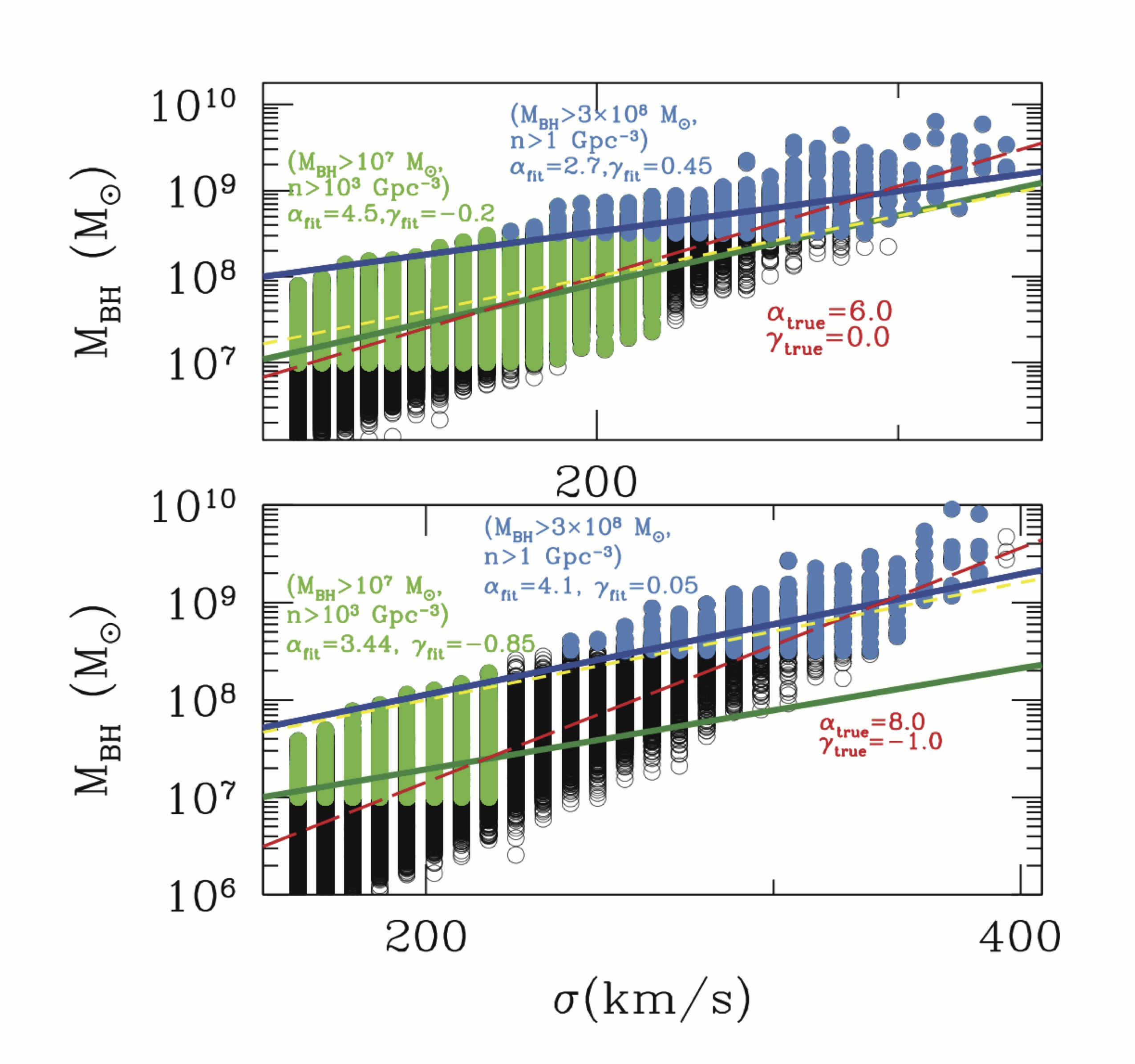
Figure 1: Top panel: $M_{\rm BH}-\sigma$ relation at $z=6$, assuming $\alpha=6$, $\gamma=0$, and a scatter of 0.25 dex. Cyan dots: ‘observable’ population in a shallow survey. Blue line: linear fit to this ‘observable’ population, yielding $\alpha=2.7$. Green dots: ‘observable’ population in a pencil-beam survey. Dark green line: linear fit to this ‘observable’ population, yielding $\alpha=4.5$. Red line: fit to the whole population, yielding $\alpha=6$. Yellow dashed line: $M_{\rm BH}-\sigma$ at $z=0$ (Equation 1 with $\alpha=4$ and $\gamma=0$). Bottom panel: same for $\alpha=8$, $\gamma=-1$.

First, we test a no-evolution case, where we set $\alpha=4$ and $\gamma=0$. We fit, in log-log space, the $M_{\rm BH}-\sigma$ relation of black holes implied by the ‘observable’ population, considering both a shallow and pencil beam survey. In the no evolution case, we find $\alpha_{\rm fit}\simeq 1$ and $\gamma_{\rm fit}\simeq 0.7$ in the ‘shallow’ survey, with almost all ‘observable’ black holes lying above the $\alpha=4$ and $\gamma=0$ line, suggesting ‘overmassive’ black holes, only because of the mass threshold that was imposed on the sample. In the ‘pencil beam’ survey we find $\alpha_{\rm fit}\simeq 2.5$ and $\gamma_{\rm fit}\simeq-0.2$. In either case, fitting only the ‘observable’ population yields a much shallower slope than that characterizing the whole population.

In Figure 1 we show a Monte Carlo simulation of the $M_{\rm BH}-\sigma$ relation at $z=6$ one would find assuming $\Delta=0.25$, $\alpha=6$ and $\gamma=0$ (top panel), and $\alpha=8$ and $\gamma=-1$ (bottom panel). In section 3, we will show that these particular choices of $\alpha$ and $\gamma$ are motivated by our attempt to fit the black hole mass function of W10. In the $\alpha=6$ and $\gamma=0$ Monte Carlo simulation, we find that the best fit has $\alpha_{\rm fit}\simeq 2.7\pm 0.2$ and $\gamma_{\rm fit}\simeq 0.45\pm 0.04$ for the ‘shallow’ survey. The apparent normalization of the relationship therefore increases by 0.35 dex (all the blue points lie above the yellow line in the top panel of figure 1). So while the underlying population is characterized only by a change in slope (with respect to the $z=0$ relationship), what would be recovered from the ‘observable’ population is a shallower slope and a positive evolution of the normalization (in agreement with point (ii) in §1). We note, additionally, that the smaller the range in $M_{BH}$ that is probed, the more likely it is that the scatter $\Delta$ hides any correlation, likely explaining the lack of correlation (point (i) in §1) found by Wang et al. (2010). If we increase the level of scatter ($\Delta$) the slope of the relationships recovered from the Monte Carlo sample becomes progressively shallower.

We can repeat the same exercise for, e.g., $\alpha=8$ and $\gamma=-1$, and although the underlying population has a much steeper slope and a negative evolution of the normalization of the $M_{\rm BH}-\sigma$ relation with redshift, the ‘observable’ population in the shallow survey would nevertheless display no evolution at all (blue vs yellow lines in Fig. 1).

Summarizing we find that, (1) selection effects can severely alter the mapping between black mass and host galaxy velocity dispersion, leading to observed black hole populations that are more massive than the true distribution. (2) Scatter and selection effects can mask correlations between black mass and host galaxy properties, leading to observed $M_{\rm BH}-\sigma$ relations that are shallower than the true relation. Although the quantitative results must be taken with caution, the existence of biases towards measuring a positive evolution in the black hole-host correlations induced by selection and scatter is generically a robust result (e.g., Shields et al. 2006, Salviander et al. 2007; Lauer et al. 2007b).

3 Impact of evolution of $M_{\rm BH}-\sigma$ relation and scatter on the black hole mass function

We now turn to the mass function of black holes, and how its shape and normalization are affected by the evolution of $M_{\rm BH}-\sigma$ relation and its scatter. We create theoretical mass functions based on Equation 1 coupled with the Press & Schechter formalism, exploring how different values of $\alpha$ and $\gamma$ influence its functional form. As discussed in section 2, one can derive relationships between black hole and dark matter halo mass given a relationship between black hole mass and velocity dispersion (Equation 1), a relationship between velocity dispersion ($\sigma$) and asymptotic circular velocity (virial velocity, $V_{c}$), and the virial theorem. For instance, assuming Equation 1 with $\alpha=4$ and $\gamma=0$, and $\sigma=V_{c}/\sqrt[]{3}$ one derives Eq. 2, while if we assume the relationship proposed by Pizzella et al. (2005) between $\sigma$ and $V_{c}$:

$$M_{\rm h}=4.1\times 10^{13}M_{\odot}\left[\frac{M_{\rm BH}}{10^{9}M_{\odot}}\right]^{0.56}\left[\frac{{\Omega_{m}}}{{\Omega_{m}^{\,z}}}\frac{\Delta_{c}}{18\pi^{2}}\right]^{-1/2}(1+z)^{-3/2}.$$ (3)

To consider the range of possible black hole mass functions, we adopt the two mappings between black hole mass and halo mass provided by Equations 2 and 3. We first consider the resulting black hole mass function when we adopt the local $M_{\rm BH}-\sigma$ relation ($\alpha=4$ and $\gamma=0$), and we will then investigate how the mass function changes if we vary $\alpha$ and $\gamma$. In particular, we will focus on $\alpha=6$ and $\gamma=0$, and $\alpha=8$ and $\gamma=-1$, because, as shown below, a steeper $M_{\rm BH}-\sigma$ relation yields better agreement between theoretical black hole mass functions and W10.

We can estimate the mass function of black holes by convolving equations 2, 3 (and their possible redshift evolution) with the mass density of dark matter halos with mass $M_{\rm h}$ derived from the Press & Schechter formalism (Sheth & Tormen 1999):

$$\frac{dN}{d\log M_{\rm BH}}=\frac{dN}{d\log M_{\rm h}}\frac{d\log M_{\rm h}}{d\log M_{\rm BH}}.$$ (4)

We assume for the time being that black holes exist in all galaxies. The effect of dropping this assumption is discussed in detail in Section 4. In figure 2 we compare the mass function derived using this technique to the mass function proposed by W10, based on the luminosity function of quasars selected by the Canada-France High-z Quasar Survey, assuming a duty cycle (corresponding to the fraction of black holes that are active, we will refer to this quantity as the active fraction, AF, below) of 0.75 and assuming a lognormal distribution of Eddington fractions, $f_{\rm Edd}$, centered at 0.6 with standard deviation of 0.30 dex (see also Shankar et al., 2010a). W10 further assume the same fraction of obscured AGN as observed at lower redshift ($z=0-2$, Ueda et al. 2003), and correct for Compton thick AGN following Shankar et al. (2009). Note that the evolution of the fraction of obscured or Compton thick AGN (currently not well constrained at high redshift, but see Treister et al. 2011) can strongly influence the results by hiding part of the black hole population (see section 4).

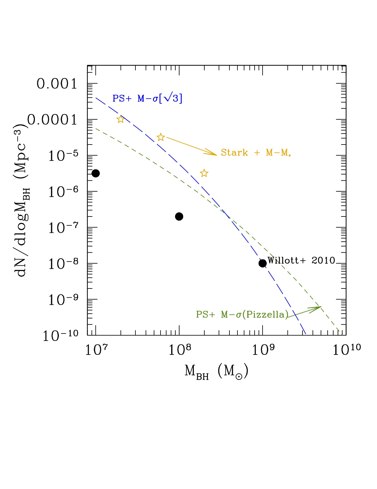
Figure 2: Mass function of black holes. Black dots: Willott et al 2010. Orange stars: $M_{\rm BH}-M_{*}$ + Stark et al. 2009 (see Willott et al. 2010 for details). Blue long dashed curve: Press & Schechter + equation 2 ($\alpha=4$). Dark green short dashed curve: Press & Schechter + equation 3 ($\alpha=4$).

If the $M_{\rm BH}-\sigma$ relation evolved with redshift as proposed by Woo et al. (2008), $\gamma=3.1$, the number density of black holes in the mass range $10^{7}-10^{9}$ M_⊙ would be $\simeq 0.5$ and $10^{-4}$ comoving Mpc^-3 respectively (the curve corresponding to this very strong evolution is not shown in the figure). We note, however, that the sample analyzed by Woo et al. (2008) is at $z\approx 0.4$, and there is no guarantee that such evolution holds at higher redshift.

In all cases the analytical models greatly over-estimate the mass function at masses $M_{\rm BH}<10^{9}$ $M_{\odot}$, and possibly at all masses – when we add the suggested positive redshift evolution of the $M_{\rm BH}-$galaxy relationships.

In figure 3 we show instead the mass function we find when we assume different $\alpha$ and $\gamma$ values, with and without scattering. We include scattering, at the level of $\Delta=0.5$, by performing a Monte Carlo simulation, where for each black hole mass we create 500 realizations of the host mass. The W10 black hole mass function can be reproduced by a simple model that has $\alpha=8$ and $\gamma=-1$, if no or little scatter in the black hole properties with galaxy mass is present. We see that as $\alpha$ increases the mass function becomes shallower. At fixed black hole mass, above the ‘hinge’ of Equation 1 (200 $\,{\rm km\,s^{-1}}$) black holes will be found in comparatively less massive galaxies, that have a higher density. On the other hand, below the ‘hinge’, the host of a black hole of a given mass would be more massive than in in the $\alpha=4$ case, hence with a lower space density. This effect makes the mass function shallower. Any decrease in $\gamma$ tends to shift the black hole mass function to lower number densities at all masses.

However, a significant amount of scatter increases the number density of observable black holes, as shown in the bottom panel of Figure 3. This effect has been discussed extensively by Lauer et al. (2007), and we refer the reader to this paper for an exhaustive demonstration of its consequences. Lauer et al. (2007) start from the luminosity function of galaxies, rather than the mass function of dark matter halos, and the fact that the most luminous galaxies are in the exponential part of the luminosity function, implies that the scattering of very high-mass black holes ($M_{\rm BH}\simeq 10^{9}$ $M_{\odot}$) in lower mass galaxies has a stronger effect than the scattering of low mass black holes in larger galaxies. A similar conclusion applies to the mass function of dark matter halos. Additionally, since the halo mass function becomes exponential at lower masses at high redshift, the effect of scatter on the shape of the black hole mass function becomes noticeable already at $M_{\rm BH}\simeq 10^{7}$ $M_{\odot}$. Including scatter, the simple model with $\alpha=8$ and $\gamma=-1$ is now a much poorer fit to W10 mass function, but it still reproduces their slope very well.

Summarizing, we find that the local $M_{\rm BH}-\sigma$ relation ($\alpha=4$ and $\gamma=0$) is unable to reproduce W10 results, even more so when a level of scatter compatible with observational results ($\Delta=0.25-0.5$) is included. A steeper $M_{\rm BH}-\sigma$ relation, with possibly a negative evolution (e.g., $\alpha=8$ and $\gamma=-1$) provides a better fit, although high levels of scatter require an even more dramatic steepening of the slope in order to match the mass function proposed by W10. While the direct comparison with W10 strongly depends on the limitations of our empirical model, the relationship between increased scatter in the $M_{\rm BH}-\sigma$ and increased number density of black holes is a robust result that directly follows from the analysis presented in Lauer et al. (2007).

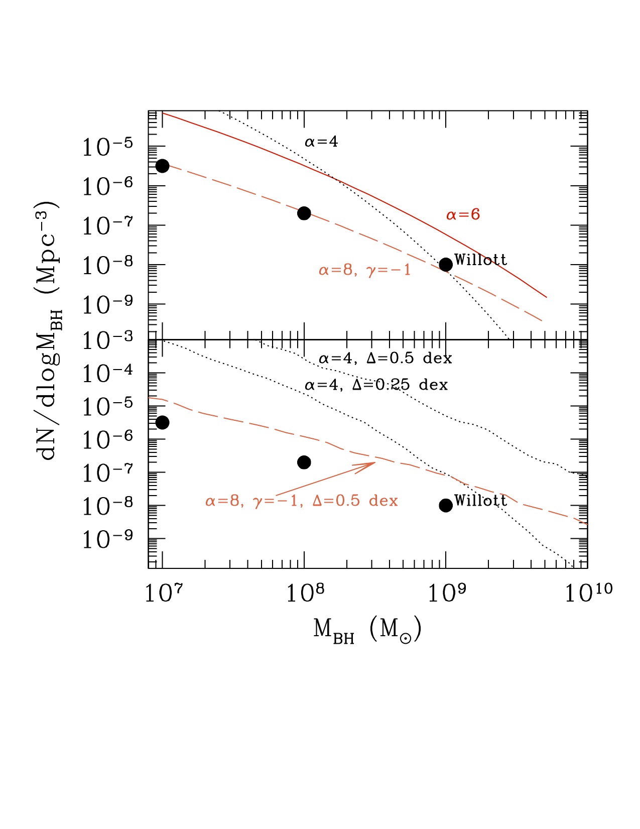
Figure 3: Mass function of black holes. Top panel: we vary the slope ($\alpha$) and normalization ($\gamma$) of the $M_{\rm BH}-\sigma$ relation, and assume no scatter in the relationship ($\Delta=0$). Bottom panel: we vary the slope of the $M_{\rm BH}-\sigma$ relation, and include scatter in the relationship ($\Delta=0.25$ dex or $\Delta=0.5$ dex). Black dots: Willott et al 2010. All curves assume Press & Schechter + equation 2, with varying $\alpha$ as labelled in the Figure.

4 Occupation fraction of quiescent and active black holes

In section 3 we demonstrated how we derive the theoretical mass function of black holes from the mass function of their host halos and the relation between black hole and halo masses (e.g., Haiman & Loeb, 1998; Wyithe & Loeb, 2002). However, when we convolve equations 2 and 3 with the mass density of dark matter halos to derive a black hole mass function, we have to make a conjecture about the fraction of halos of a given mass which host a black hole, the occupation fraction (OF):

$$\frac{dN}{d\log M_{\rm BH}}={\rm OF}(M_{\rm h},z)\frac{dN}{d\log M_{\rm h}}\frac{d\log M_{\rm h}}{d\log M_{\rm BH}}.$$ (5)

In the top panel of Fig. 4 we show black hole mass functions resulting from different choices of the OF. It is clear that a decreasing OF can compensate for an increased scatter in shaping the black hole mass function. As a result of this degeneracy, we can reproduce the W10 mass function for a range of values for the OF and scatter. Even adopting $\alpha=4$ (slope of $M_{\rm BH}-\sigma$ relation at the present day) with a sensible scatter can fit the data, at the cost, however, of making the presence of a black hole (regardless of its shining as a quasar) a very rare instance. We note that it is conceivable that the OF is not constant over all host masses, and a non trivially constant OF is expected particularly at high-redshift, close to the epoch of galaxy and black hole formation (Menou et al., 2001). At face value, the W10 data can be reproduced by OF$=M_{\rm h}/5\times 10^{13}$ $M_{\odot}$for $\alpha=4$, $\gamma=0$ and $\Delta=0.25$, or OF$=(M_{\rm h}/10^{13}$$M_{\odot}$$)^{1.25}$ for $\alpha=4$, $\gamma=0$ and $\Delta=0$. Such occupation fractions are several orders of magnitude lowers than predicted by models of formation and cosmic evolution of black holes (e.g., Volonteri, 2010), and we therefore still prefer solutions with steeper slopes. We will explore self-consistently OF and its relationship with the establishment of the $M_{\rm BH}-\sigma$ relation as a function of black hole formation and growth physics in a future paper.

Throughout this paper we have compared our theoretical mass function of black holes to constraints derived indirectly from the luminosity function of quasars in W10, rather than from direct black hole mass measurements (that are rather unfeasible at $z=6$). Empirically, one can derive the mass function of black holes from the luminosity function of quasars and a relation between black hole mass and quasar luminosity (e.g., Shankar et al., 2010a, b; Willott et al., 2010):

$$\frac{dN}{d\log M_{\rm BH}}=\frac{dN}{d\log L}\frac{d\log L}{d\log M_{\rm BH}}.$$ (6)

For instance, we can estimate the mass function of black holes from the bolometric luminosity of radio-quiet quasars (Hopkins et al., 2007) assuming (1) that all black holes are active, (2) that all black holes radiate at the same Eddington fraction, $f_{\rm Edd}$ (based on various observational results we expect high redshift quasars to radiate close to the Eddington limit, see W10 and references therein). The mass of a black hole powering a quasar with luminosity $L$ is then:

$$\frac{M_{\rm BH}}{10^{9}M_{\odot}}=3\times 10^{-14}\frac{1}{f_{\rm Edd}}\frac{L}{L_{\odot}},$$ (7)

and one can trivially turn the luminosity function into a mass function. As discussed by W10, their mass function is derived assuming similar values of the Eddington ratio and the active fraction using a more accurate technique (see Shankar et al., 2010a, for details). Our simple approach provides results consistent with W10 if we assume a constant $f_{\rm Edd}=1$.

When we deconvolve the luminosity function of quasars to derive the black hole mass function we have to assume an active fraction (AF):

$$\frac{dN}{d\log M_{\rm BH}}={\rm AF}(M_{\rm BH},z)\frac{dN}{d\log L}\frac{d\log L}{d\log M_{\rm BH}},$$ (8)

where we indicate that both the active fraction and the Eddington ratio can be functions of the black hole (and host) properties, and of cosmic time.

The intrinsic shape of the mass function changes as a function of AF and $f_{\rm Edd}$, and, in particular, any departure from the assumptions $f_{\rm Edd}=1$ and AF$=1$ (that are upper limits to both quantities) will drive the mass function of black holes ‘up’, that is, they will increase the number of black holes at a given mass. We have therefore to bear in mind that the semi-empirical mass function derived by W10 might be underestimating the mass function. The lower panel of Fig. 4 shows how the mass functions one derives from a luminosity function are modified by an AF or $f_{\rm Edd}$ that depend on the BH mass. For instance, we can trivially assume that $f_{\rm Edd}=M_{BH}/10^{8}$ $M_{\odot}$  for $M_{BH}<10^{8}$ $M_{\odot}$, and $f_{\rm Edd}=1$ otherwise. Then $M_{\rm BH}=10^{8}M_{\odot}(L/3\times 10^{12}L_{\odot})^{0.5}$, using equation 7 in the last expression. In the same figure we also show the effect of a mass dependent AF, where we adopt the simple expression AF$=M_{BH}/10^{8}$ $M_{\odot}$  for $M_{BH}<10^{8}$ $M_{\odot}$, and AF$=1$ otherwise. These specific forms of the mass dependence of AF and $f_{\rm Edd}$ are motivated by the expectation that the most massive black holes at the earliest cosmic times are all actively and almost constantly accreting (Haiman, 2004; Shapiro, 2005; Volonteri & Rees, 2005, 2006). Such functional forms are here only used to prove that non constant accretion rates modify the expectations in terms of mass function and active fraction, but the expressions we adopt should be considered representative of any class of accretion rates and active fractions that are not constant, rather than actual predictions.

If the Eddington ratio and/or AF are a function of halo or black hole mass, then what one derives from flux-limited surveys will be dependent on a combination of various properties. Figure 5 shows simple examples. We build a sample of black holes and hosts by performing a Monte Carlo sampling as described in Section 3 for two $M_{\rm BH}-\sigma$ relations ($\alpha=4$ and $\alpha=6$, both with $\gamma=0$) each with a scatter of 0.25 dex. We assign to each black hole a luminosity by assuming either a constant $f_{\rm Edd}=1$, or that $f_{\rm Edd}=M_{BH}/10^{8}$ $M_{\odot}$  or $M_{BH}<10^{9}$  $M_{\odot}$  and $f_{\rm Edd}=$1 for $M_{BH}>10^{8}$  $M_{\odot}$(we note that the assumption that $f_{\rm Edd}$ scales with the halo mass, rather than the black hole mass, yields very similar results). Even for a constant Eddington ratio, scatter in the $M_{\rm BH}-\sigma$ relation implies that at fixed halo mass the black hole mass and hence its luminosity is not univocally determined. The ‘observed’ active population of black holes will therefore be different from the ‘intrinsic’ active fraction, which in this exercise was set to unity. A comparison between the left and right panels underscores how the $M_{\rm BH}-\sigma$ relation itself shapes the fraction of active black holes which are detected in optical imaging surveys.

We notice that obscuration plays a role similar to the occupation or active fraction. If, say, all black holes are active, but a large fraction are Compton thick, then a large population of obscured quasars would be unaccounted for in optical quasar surveys. There is indeed evidence for a large fraction of high redshift quasars being obscured (e.g., La Franca et al., 2005; Treister et al., 2009, 2011).

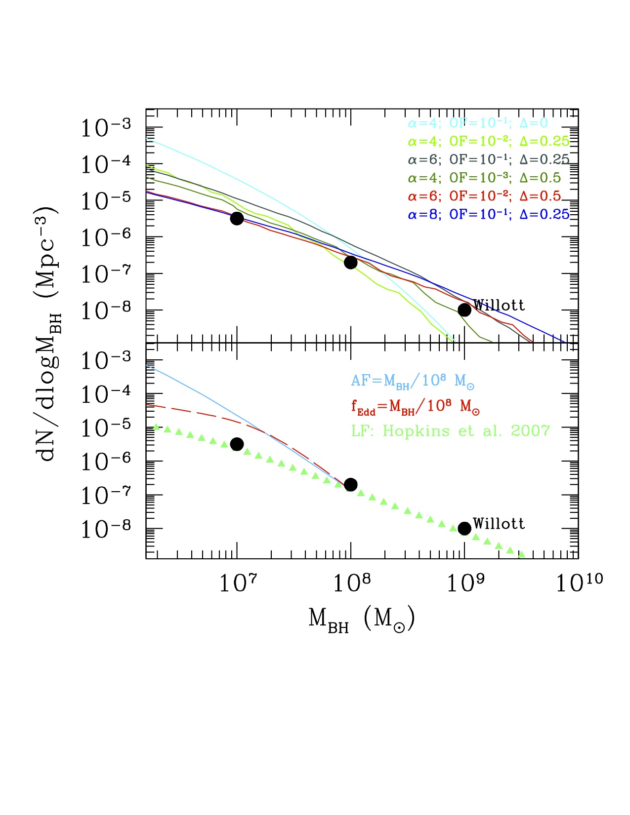
Figure 4: Top: theoretical mass function of black holes derived from the mass function of dark matter halos (Eq. 5). Black dots: Willott et al 2010. Other curves as marked in the figure (from top to bottom). Willott et al. results can be reproduces for a range of possible assumptions on the relation between holes and halos. Bottom: empirical mass function of black holes derived from the luminosity function of quasars (Eq. 7 and Eq. 8, adopting the bolometric luminosity function of Hopkins et al. 2007). Triangles: $f_{\rm Edd}=1$ and $AF=1$. The blue solid and red dashed curves show how mass-dependent luminosities or active fractions can modify the shape of the mass function one would infer.

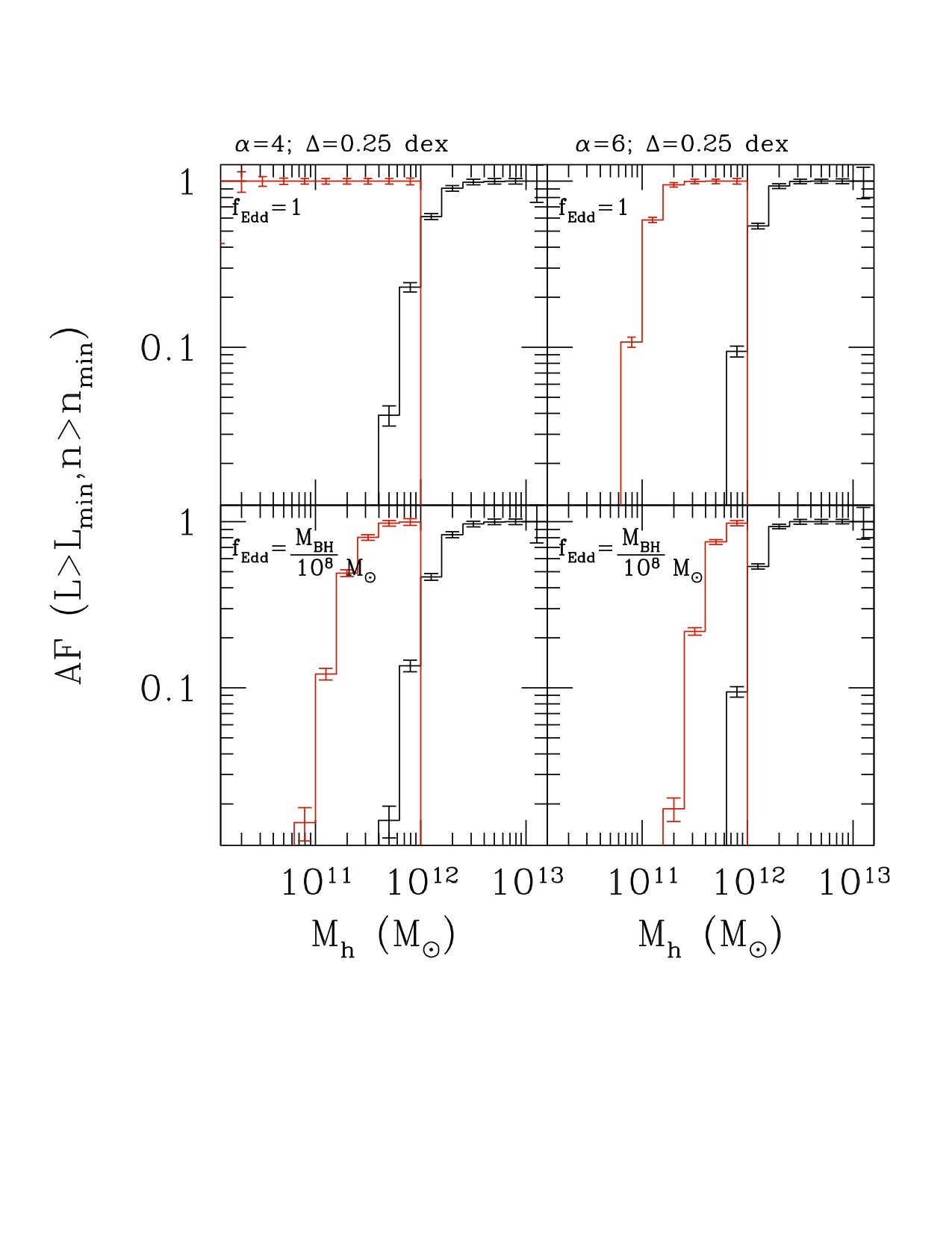
Figure 5: Fraction of active black holes than can be detected in a survey with given luminosity and volume limit. Red histograms (leftmost side of each panel): black holes with $L_{\rm min}=10^{44}$ erg/s and $n_{\rm min}=10^{-5}$ Mpc^-3 (example of a pencil beam survey). Black histograms (rightmost side of each panel): black holes with $L_{\rm min}=10^{46}$ erg/s and $n_{\rm min}=10^{-9}$ Mpc^-3 (example of a shallow survey). Left panels: $\alpha=4$; $\Delta=$0.25 dex. Right panels: $\alpha=6$; $\Delta=$0.25 dex. Top panels: $f_{\rm Edd}=1$. Bottom panels: $f_{\rm Edd}=M_{BH}/10^{8}$ $M_{\odot}$.

5 Accretion efficiency and host mass

In the previous section we discussed how the ‘observed’ fraction of active black holes, which goes into determining the ‘observed’ mass function depends on the $M_{\rm BH}-\sigma$ relationship and on the link between accretion rate and black hole-host masses. In this section, we explore the consequences and likelihood of a galaxy mass-dependent black hole accretion rate. This hypothesis is plausible, as the gas supply, especially at high redshift is likely dependent on the environment and mass of the host. For instance cold gas that flows rapidly to the center of galaxies from filaments around haloes plays a major role in the buildup of massive galaxies at high redshift (Brooks et al., 2009; Governato et al., 2009), with a transition expected to occur when a galaxy has mass above $10^{11}$$M_{\odot}$, where gas is shocked before it can reach the galaxy’s disk. Cold gas flowing into halos along large-scale structure filaments may however be dense enough to penetrate the shock front and deliver cold gas to the galaxy. Galaxies that form within a gas-rich filament will accrete gas from this cold flow and grow substantially before the filament dissipates. These galaxies embedded in filaments are expected to be high peaks of the density field, hence among the most massive at early times.

Additionally, as discussed in section 3, instead of an overall normalization evolution, the link between black holes and their hosts might be better explained by an evolution in the slope of the $M_{\rm BH}-\sigma$ relationship. We are not claiming here that the evolution has the exact form that we use in this paper (Equation 1). We here discuss a possible physical scenario that can lead to a steeper $M_{\rm BH}-\sigma$ relation.

In the following toy model we just explore what physical process could drive the establishment of a given $M_{\rm BH}-\sigma$ relation at a given redshift ($z=6$ in this particular case). In other words, if the slope of the $M_{\rm BH}-\sigma$ relation at $z=6$ has a given $\alpha$, what can be the driver of such correlation?

Let us assume that all black holes start with the same initial mass, $M_{0}$, and let them grow until $z=6$ ($t_{H}=0.9$ Gyr). If at $z=6$ the slope of the $M_{\rm BH}-\sigma$ relationship is $\alpha$, and we assume that on average black holes accrete at a fraction $\langle f_{\rm Edd}\rangle$ of the Eddington rate, then we can relate this average accretion rate of the mass of the hole, $M_{\rm BH,6}$ and the velocity dispersion, $\sigma_{6}$, of the host at $z=6$, as follows:

$$M_{\rm BH,6}=M_{0}\exp\left({\langle f_{\rm Edd}\rangle\frac{t_{H}}{t_{\rm Edd}}\frac{1-\epsilon}{\epsilon}}\right),$$ (9)

where $t_{\rm Edd}=M_{\rm BH}c^{2}/L_{\rm Edd}=\frac{\sigma_{T}\,c}{4\pi\,G\,m_{p}}=0.45$ Gyr ($c$ is the speed of light, $\sigma_{T}$ is the Thomson cross section, $m_{p}$ is the proton mass), and the radiative efficiency, $\epsilon\simeq 0.1$. We can also express the relationship between black hole mass $M_{\rm BH,6}$ and $\sigma_{6}$ at $z=6$ as:

$$\sigma_{6}=200\,{\rm km\,s^{-1}}\left(\frac{M_{\rm BH,6}}{10^{8}\,{\rm M_{\odot}}}\right)^{1/\alpha},$$ (10)

so that the average accretion rate for a black hole that grows within a galaxy that has a velocity dispersion $\sigma_{6}$ at $z=6$ results:

$$\langle f_{\rm Edd}\rangle=\frac{t_{\rm Edd}}{t_{H}}\frac{\epsilon}{1-\epsilon}\ln\left[\left(\frac{10^{8}\,{\rm M_{\odot}}}{M_{0}}\right)\left(\frac{\sigma_{6}}{200\,{\rm km\,s^{-1}}}\right)^{\alpha}\right].$$ (11)

Equations 9–11 are based on the initial conditions and on the properties at $z=6$ only. The accretion rate is in principle galaxy–mass dependent, and specifically dependent also on the mass growth of the host. However, for the sake of simplicity it is here set to the average over the integration time.

The average accretion rate of Eq. 11 is shown in Figure 6 for $\alpha=4$, $\alpha=6$ and $\alpha=8$. Figure 6 implies that if only black holes in hosts above a certain velocity dispersion, or mass, or depth of the potential well, can accrete efficiently, it is only natural to expect a different slope of the $M_{\rm BH}-\sigma$ relationship in dependence of the exact threshold. One possibility is that black hole growth is indeed inefficient in low-mass galaxies at early cosmic times, because of the fragile environment where feedback can be very destructive (Milosavljević et al., 2009; Alvarez et al., 2009; Park & Ricotti, 2010; Johnson et al., 2010). We note that all these possible scalings of accretion rate with halo mass are consistent with the independence of $f_{\rm Edd}$ on luminosity (and black hole mass) found by W10, as all their black holes have masses above $10^{8}\,{\rm M_{\odot}}$, where it is indeed expected that the accretion rate can reach $f_{\rm Edd}\simeq 1$ as one can infer from Figure 6.

This exercise is not meant to suggest that the typical accretion rate has the exact value of Eq. 9, but that if accretion is more efficient in more massive halos, then $\alpha$ increases, while if the accretion rate is mass independent, e.g. is constant in all hosts, then $\alpha$ tends to lower values.

Equation 11 simply demonstrates mathematically that in order to achieve a very steep $M_{\rm BH}-\sigma$ accretion in massive haloes has to be more efficient than in small haloes (‘selective accretion’), and it should not be used to make predictions about the accretion/growth history of black holes. To test this suggestion, dedicated simulations that can resolve the growth of black holes in cosmological simulations as a function of the host mass are required. However, simulations that explore the cosmic evolution of accretion efficiency, taking into consideration feeding and feedback, as a function of host mass at sufficient resolution are not currently available.

The experiment that is closest in spirit to what we propose was performed by Pelupessy et al. (2007) who suggest that the more massive the host halo, the higher the Eddington fraction. A very simple fit from their simulation results at $z=6$ (Figure 7 in Pelupessy et al. 2007) gives:

$$f_{\rm Edd}\approx\frac{M_{\rm h}}{10^{11}\,{\rm M_{\odot}}}.$$ (12)

This equation is shown in Figure 6 for different hosts, where we assumed $\sigma=V_{c}/\sqrt[]{3}$, and that the Eddington limit is capped at $f_{\rm Edd}=1$ (in the bottom panel the black hole mass uses Equation 9). This scaling leads to very steep relationships between black holes and hosts, as shown in the bottom panel of Figure 6, as the black hole mass depends exponentially on the halo mass (if we insert equation 12 into equation 9) or on the time evolution of the halo mass (if we insert equation 12 into the expression for the accretion rate in Eddington units: $\dot{M}=f_{\rm Edd}(M/t_{\rm Edd})[(1-\epsilon)/\epsilon]=(M_{\rm h}(t)/10^{11})(M/t_{\rm Edd})[(1-\epsilon)/\epsilon]$. To integrate this equation properly one needs to know the growth rate of the host dark matter halo mass as a function of time in a $\Lambda$CDM cosmology, $M_{\rm h}(t)$. Such exercise requires either merger trees that track the cosmic history of dark matter halos, or an analytical fit to their growth histories, and it is beyond the scope of this paper). Selective accretion, modulated by the host’s potential and environment, is a possible key to explaining a shallow high redshift black hole mass function without requiring an unrealistically low occupation fraction.

At late cosmic times we expect the interaction of black holes and galaxies to become more closely linked to baryonic processes (e.g., bulge formation) rather than being related to the halo mass. For instance, secular effects might at late times decouple the properties of the central stellar-dominated region from the overall dark matter halo. As another example, gas accretion through cold flows in filaments is expected to occur only at early times. We can, for instance, see a parallel between the black hole-halo relationship and the baryon-halo relationship. It is expected that at very high redshift most halos possess a baryon fraction of order the cosmic baryon fraction, while at later times the baryonic content evolves under the effect of baryonic physics. In the same way at late times we expect black hole growth to be more closely related to the baryonic content of a galaxy, and hence less “selectively” linked to the host halo (cf. Volonteri et al. 2011).

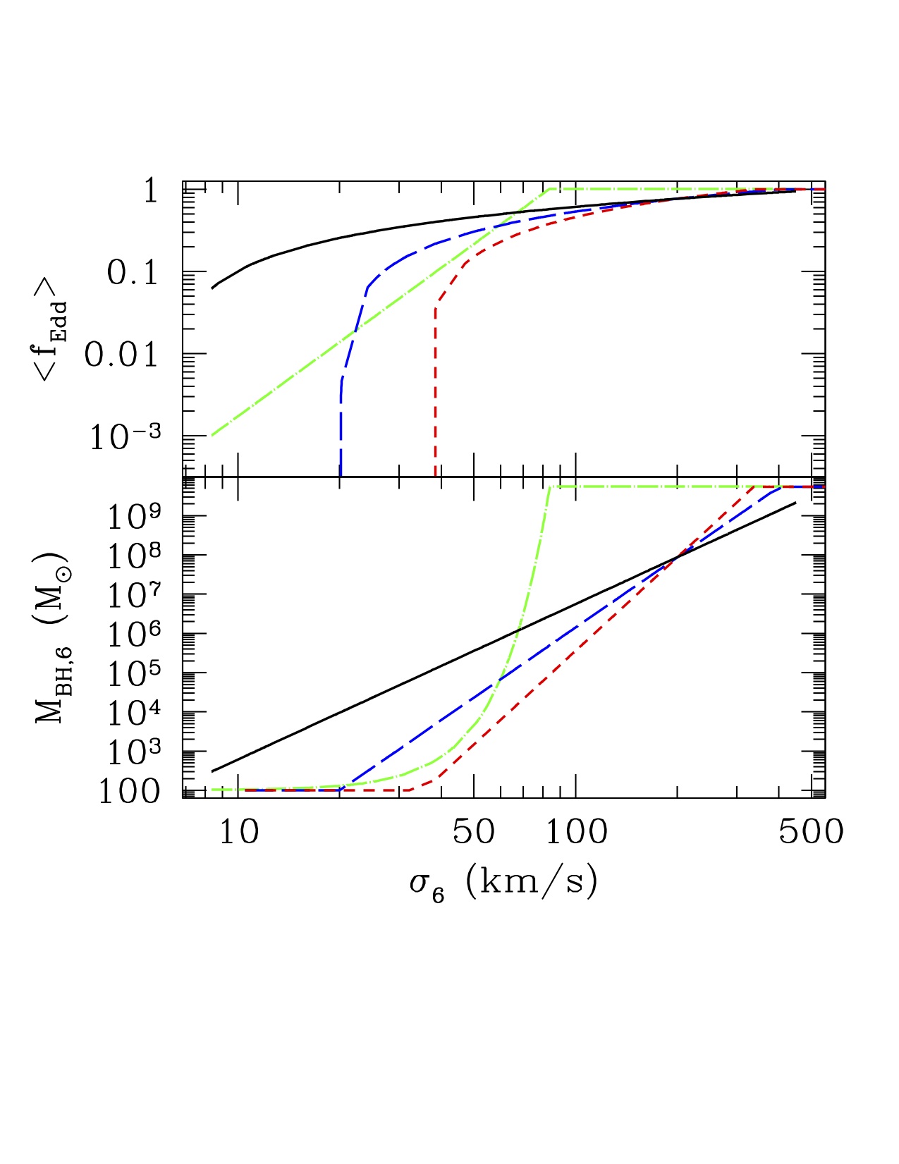
Figure 6: Top: Eddington fraction as a function of halo velocity dispersion, derived from equation 11 (black solid: $\alpha=4$; blue long dashed: $\alpha=6$; red short dashed: $\alpha=8$) and equation  12 (green dot-dashes). Bottom: black hole mass versus $\sigma$ at $z=6$ assuming $f_{\rm Edd}$ is a function of halo properties, and letting the holes accrete for $t_{H}=0.9$ Gyr.

6 Summary and conclusions

Recent observational results that focus on high-redshift black holes provide seemingly conflicting results. In particular:

• there seems to be little or no correlation with velocity dispersion, $\sigma$ in the brightest radio-selected quasars,

• typically black holes are ‘over-massive’ at fixed galaxy mass/velocity dispersion compared to their $z=0$ counterparts,

• clustering and analysis of the mass/luminosity function suggest that either many massive galaxies do not have black holes, or these black holes are less massive than expected.

To try and understand these observational results, we explore the role of scatter and observational biases in recovering the intrinsic properties of the black hole population. We generate Monte Carlo realizations of the $M_{\rm BH}-\sigma$ relation at $z=6$, varying the slope and normalization, and select ‘observable’ systems from these samples, considering either ‘shallow’ or ‘pencil beam’ surveys. We test how well we can recover the parameters of the $M_{\rm BH}-\sigma$ relation from the ‘observable’ systems only. We then create theoretical mass functions of black holes from the mass function of halos and $M_{\rm BH}-\sigma$ and test what assumptions can reproduce the mass function derived by W10. Our techniques are very simplified and we use empirical correlations that are not guaranteed to hold at all masses and reshifts. Therefore one should not interpret our results as solutions to the three conflicting points mentioned above, but rather regard them as a way for understanding how different physical parameters may affect black hole related quantities and their measurements.

Our results can be summarized as follows:

• Scatter and bias selections can hide the intrinsic correlations between holes and hosts. When selecting within a small range in black hole and galaxy masses, at the high-mass end, the scatter washes out correlations (see point (i) above), and most of the selected systems will tend to lie above the underlying correlation. The correlations recovered from ‘observable’ sub-samples of the whole population can therefore suggest positive evolution even when the underlying population is characterized by no or negative evolution.

• The slope and normalization of the local $M_{\rm BH}-\sigma$ correlation are unable to produce a black hole mass function compatible with W10, as the theoretical mass function greatly overstimates the density of black holes with $M_{\rm BH}<10^{8}$. The discrepancy can be minimized if very few halos (of order 1/1000) host a massive black hole or an AGN at $z=6$, or most AGN at these redshift are obscured. $M_{\odot}$.

• If the $M_{\rm BH}-\sigma$ correlation were steeper at $z=6$, then at fixed black hole mass high mass black holes would reside in comparatively less massive galaxies than in the $\alpha=4$ case. Their number density is therefore increased. Viceversa, low mass black holes would be hosted in comparatively larger galaxies (compare red and yellow lines in Figure 1) with a lower space density. This effect helps reproducing the mass function of $z=6$ black holes proposed by W10.

• On the other hand, scatter in the $M_{\rm BH}-\sigma$, at the level of what is observed locally, exacerbates the discrepancy, as it increases the number density of black holes at $M_{\rm BH}>10^{7}$ $M_{\odot}$. Any type of positive evolution of the $M_{\rm BH}-\sigma$ exacerbates this discrepancy.

• Analysis of AGN samples might be underestimating the black holes mass function at low masses if the active fraction or luminosity are a function of host or black hole mass.

In the near future the synergy of JWST and ALMA can zoom in on quasars and their hosts respectively informing us of their relationship and how the $M_{\rm BH}-\sigma$ relation is established, or how the accretion properties depend on the black hole or halo mass. In the near-IR, JWST will have the technical capabilities to detect quasars at $z\mathrel{\hbox to0.0pt{\lower 3.0pt\hbox{$\sim$}\hss}\raise 2.0pt\hbox{$>$}}6$ down to a mass limit as low as $10^{5}-10^{6}$ $M_{\odot}$, owing to its large field of view and high sensitivity. At the expected sensitivity of JWST, $\simeq 1$ nJy, almost $7\times 10^{3}$ deg^-2 sources at $z>6$ should be detected (Salvaterra et al., 2007). At the same time, the exquisite angular resolution and sensitivity of ALMA can be used in order to explore black hole growth up to high redshift even in galaxies with high obscuration and active star formation. To date the best studies of the hosts of $z\simeq 6$ quasar have been performed at cm-wavelength (Walter et al., 2004; Wang et al., 2010). The best studied case is J1148+5251 at z = 6.42. The host has been detected in thermal dust, non-thermal radio continuum, and CO line emission (Bertoldi et al., 2003; Carilli et al., 2004; Walter et al., 2004). ALMA will be able to detect the thermal emission from a source like J1148+5251 in a few seconds at sub-kpc resolution (Carilli et al., 2008). On a similar time-frame Dark-Energy oriented survey will provide an enormous amount of quasar data as ancillary science (e.g. DES, LSST). Coupling the information we derive from these extremely large yet shallow surveys, with that derived from deep pencil beam surveys will undoubtedly deepen our understanding of the growth of high-redshift black holes.

In the meantime, we need to develop dedicated cosmological simulations of black hole formation and early growth that can aid the interpretation of these data. The suggestion that the accretion rate of massive black holes depends on their environment, (through the host halo and its cosmic bias) must be tested with cosmological simulations that implement physically-motivated accretion and feedback prescriptions. We also need to derive predictions for the occupation fraction of black holes in galaxies based on black hole formation models (Bellovary et al. in prep.). This will be a significant improvement over current simulations of black hole cosmic evolution that typically place black holes in halos growing above some threshold mass, typically $\sim 10^{10}$ $M_{\odot}$, leading to a trivial occupation fraction function. There is no strong physical reason to believe that all and only galaxies with mass $>10^{10}$$M_{\odot}$  host massive black holes in their centers.

In this paper we focused on the very high-redshift Universe, $z\simeq 6$. Although this redshift range is not a special place, the concurrence of theoretical arguments and observational constraints allow us to make simplifying assumptions that are not expected to be valid at later times. For instance, a timescale argument requires black holes to grow fast to reach the masses probed by current luminosity functions. In turn, this argument, coupled to current observational constraints suggest that the most luminous quasars accrete close to Eddington, and that both active fraction and occupation fractions must be of order unity at the high-luminosity, high-mass end. This is not true at $z=2$, where more variables enter into play, and make the analysis less constraining. An example of a detailed study that connects the mass function of black holes derived from the Press & Schechter formalism to that derived from the luminosity function is presented in Croton (2009).

References

- Adelberger & Steidel (2005) Adelberger, K. L., & Steidel, C. C. 2005, ApJ, 627, L1
- Alvarez et al. (2009) Alvarez M. A., Wise J. H., Abel T., 2009, ApJ, 701, L133
- Bertoldi et al. (2003) Bertoldi, F., et al. 2003, A&A, 409, L47
- Binney & Tremaine (2008) Binney, J., & Tremaine, S. 2008, Galactic Dynamics: Second Edition, by James Binney and Scott Tremaine. ISBN 978-0-691-13026-2 (HB). Published by Princeton University Press, Princeton, NJ USA, 2008.,
- Bluck et al. (2010) Bluck, A. F. L., Conselice, C. J., Almaini, O., Laird, E. S., Nandra, K., & Grützbauch, R. 2011, MNRAS, 410, 1174
- Brooks et al. (2009) Brooks, A. M., Governato, F., Quinn, T., Brook, C. B., & Wadsley, J. 2009, ApJ, 694, 396
- Carilli et al. (2004) Carilli, C. L., et al. 2004, AJ, 128, 997
- Carilli et al. (2008) Carilli, C. L., et al. 2008, Ap&SS, 313, 307
- Croton (2009) Croton D. J., 2009, MNRAS, 394, 1109
- Decarli et al. (2010) Decarli, R., Falomo, R., Treves, A., Labita, M., Kotilainen, J. K., & Scarpa, R. 2010, MNRAS, 402, 2453
- Fine et al. (2006) Fine, S., et al. 2006, MNRAS, 373, 613
- Governato et al. (2009) Governato, F., et al. 2009, MNRAS, 398, 312
- Gültekin et al. (2009) Gültekin K., Richstone D. O., Gebhardt K., Lauer T. R., Tremaine S., Aller M. C., Bender R., Dressler A., Faber S. M., Filippenko A. V., Green R., Ho L. C., Kormendy J., Magorrian J., Pinkney J., Siopis C., 2009, ApJ, 698, 198
- Haiman & Loeb (1998) Haiman, Z., & Loeb, A. 1998, ApJ, 503, 505
- Haiman (2004) Haiman, Z. 2004, ApJ, 613, 36
- Hopkins et al. (2007) Hopkins, P. F., Richards, G. T., & Hernquist, L. 2007, ApJ, 654, 731
- Jahnke et al. (2009) Jahnke, K., et al. 2009, ApJ, 706, L215
- Johnson et al. (2010) Johnson, J. L., Khochfar, S., Greif, T. H., & Durier, F. 2011, MNRAS, 410, 919
- Kormendy & Bender (2011) Kormendy, J., & Bender, R. 2011, Nat, 469, 377
- La Franca et al. (2005) La Franca, F., et al. 2005, ApJ, 635, 864
- Lauer et al. (2007) Lauer T. R., Faber S. M., Richstone D., Gebhardt K., Tremaine S., Postman M., Dressler A., Aller M. C., Filippenko A. V., Green R., Ho L. C., Kormendy J., Magorrian J., Pinkney J., 2007a, ApJ, 662, 808
- Lauer et al. (2007) Lauer T. R., Tremaine S., Richstone D., Faber S. M., 2007b ApJ, 670, 249
- McLure & Dunlop (2004) McLure R. J., Dunlop J. S., 2004, MNRAS, 352, 1390
- Menou et al. (2001) Menou, K., Haiman, Z., & Narayanan, V. K. 2001, ApJ, 558, 535
- Merloni (2010) Merloni A. et. al, 2010, ApJ, 708, 137
- Milosavljević et al. (2009) Milosavljević M., Couch S. M., Bromm V., 2009, ApJ, 696, L146
- Park & Ricotti (2010) Park K., Ricotti M., 2010, ArXiv e-prints
- Pelupessy et al. (2007) Pelupessy F. I., Di Matteo T., Ciardi B., 2007, ApJ, 665, 107
- Peng et al. (2006) Peng C. Y., Impey C. D., Rix H.-W., Kochanek C. S., Keeton C. R., Falco E. E., Lehár J., McLeod B. A., 2006, ApJ, 649, 616
- Pizzella et al. (2005) Pizzella, A., Corsini, E. M., Dalla Bontà, E., Sarzi, M., Coccato, L., & Bertola, F. 2005, ApJ, 631, 785
- Salvaterra et al. (2007) Salvaterra, R., Haardt, F., & Volonteri, M. 2007, MNRAS, 374, 761
- Salviander et al. (2007) Salviander, S., Shields, G. A., Gebhardt, K., & Bonning, E. W. 2007, ApJ, 662, 131
- Shen et al. (2008) Shen Y., Greene J. E., Strauss M. A., Richards G. T., Schneider D. P., 2008, ApJ, 680, 169
- Schneider et al. (2010) Schneider, D. P., et al. 2010, AJ, 139, 2360
- Shankar et al. (2009) Shankar, F., Weinberg, D. H., & Miralda-Escudé, J. 2009, ApJ, 690, 20
- Shankar et al. (2010a) Shankar, F., Crocce, M., Miralda-Escudé, J., Fosalba, P., & Weinberg, D. H. 2010, ApJ, 718, 231
- Shankar et al. (2010b) Shankar, F., Weinberg, D. H., & Shen, Y. 2010, MNRAS, 406, 1959
- Shapiro (2005) Shapiro, S. L. 2005, ApJ, 620, 59
- Shen & Kelly (2010) Shen, Y., & Kelly, B. C. 2010, ApJ, 713, 41
- Shields et al. (2006) Shields, G. A., Menezes, K. L., Massart, C. A., & Vanden Bout, P. 2006, ApJ, 641, 683
- Sijacki et al. (2009) Sijacki D., Springel V., Haehnelt M. G., 2009, MNRAS, 400, 100
- Treister et al. (2009) Treister, E., Urry, C. M., & Virani, S. 2009, ApJ, 696, 110
- Treister et al. (2011) Treister, E., Schawinski, K., Volonteri, M., Natarajan, P., & Gawiser, E. 2011, Nat, 474, 356
- Ueda et al. (2003) Ueda, Y., Akiyama, M., Ohta, K., & Miyaji, T. 2003, ApJ, 598, 886
- Vestergaard et al. (2008) Vestergaard M., Fan X., Tremonti C. A., Osmer P. S., Richards G. T., 2008, ApJ, 674, L1
- Volonteri & Rees (2005) Volonteri, M., & Rees, M. J. 2005, ApJ, 633, 624
- Volonteri & Rees (2006) Volonteri, M., & Rees, M. J. 2006, ApJ, 650, 669
- Volonteri (2010) Volonteri, M. 2010, A&A Rev., 18, 279
- Volonteri et al. (2011) Volonteri, M., Natarajan, P., & Gultekin, K. 2011, arXiv:1103.1644
- Walter et al. (2004) Walter F., Carilli C., Bertoldi F., Menten K., Cox P., Lo K. Y., Fan X., Strauss M. A., 2004, ApJ, 615, L17
- Wang et al. (2010) Wang R., Carilli C. L., Neri R., Riechers D. A., Wagg J., Walter F., Bertoldi F., Menten K. M., Omont A., Cox P., Fan X., 2010, ApJ, 714, 699
- Willott et al. (2010) Willott C. J., Albert L., Arzoumanian D., Bergeron J., Crampton D., Delorme P., Hutchings J. B., Omont A., Reylé C., Schade D., 2010, AJ, 140, 546 (W10)
- Woo et al. (2008) Woo J., Treu T., Malkan M. A., Blandford R. D., 2008, ApJ, 681, 925
- Wyithe & Loeb (2002) Wyithe, J. S. B., & Loeb, A. 2002, ApJ, 581, 886