Numerical simulation of two-dimensional Faraday waves with phase-field modelling

Abstract

A fully nonlinear numerical simulation of two-dimensional Faraday waves between two incompressible and immiscible fluids is performed by adopting the phase-field method with the Cahn-Hilliard equation due to Jacqmin (J. Comput. Phys., vol. 155, 1999, pp. 96-127). Its validation is checked against the linear theory. In the nonlinear regime, qualitative comparison is made with an earlier vortex-sheet simulation of two dimensional Faraday waves by Wright , Yon & Pozrikidis (J. Fluid Mech., vol. 400, 2000, pp. 1-32). The vorticity outside the interface region is studied in this comparison. The period tripling state, which is observed in the quasi-two dimensional experiment by Jiang, Perlin & Schultz (J. Fluid Mech., vol. 369, 1998, pp. 273-299), is successfully simulated with the present phase-field method.

1 Introduction

Faraday waves, which typically refer to complex patterns of standing waves on a fluid surface in an oscillating container, are among the classical problems of fluid mechanics (Faraday, 1831). The phenomenon has been a representative example of parametric instabilities (Miles & Henderson, 1990). As is often the case with fluid mechanics, even classical phenomena are often not well understood in nonlinear regimes. Indeed, continuing experiments on Faraday waves beyond the linear regimes reveal intriguing new features, which include snake-like structures in drop-confined Faraday waves (Pucci, Fort, Ben Armar & Couder, 2011), a turbulent state mediated by defects of the pattern (Shani, Cohen & Fineberg, 2010) and so-called oscillons (Arbell & Fineberg, 2000).

These surprising findings would probably be outside of the applicable range of the weakly nonlinear theories, such as the one developed by Chen & Viñals (1999), on selection of various patterns of Faraday waves. Hence, to understand these phenomena, fully nonlinear numerical simulations of the Faraday systems, which can be complementary to laboratory experiments, play an indispensable role as discussed in Kityk, Embs, Mekhonoshin & Wagner (2005). Perhaps the first such simulation, in which the motions of both the top and bottom fluids are simultaneously simulated, was performed recently by Périnet, Juric & Tuckerman (2009). This motivates our present study.

In these fully nonlinear simulations, the inevitable difficulties are how to represent numerically the interface between the two immiscible fluids, how to follow its motion and how to calculate its influence on the bulk fluids. In Périnet, Juric & Tuckerman (2009), the interface is modelled by triangular elements whose apices are advected vertically and data on the interface elements are copied to the Eulerian grids in the bulk of the fluids according to the recipe of the immersed boundary method (Peskin, 1977). Since numerical modelling of the interface involves various assumptions, its validation is required against laboratory experimental data or other data independent of the modelling. In the linear regime, the analytical result of the linear theory of Faraday waves due to Kumar & Tuckerman (1994) provides reliable data for comparison, as used in Périnet, Juric & Tuckerman (2009). In nonlinear regimes, comparison with experimental data is crucial. Remarkably, the simulation result by Périnet, Juric & Tuckerman (2009) is in perfect agreement with the experimental data in the nonlinear regime conducted by Kityk, Embs, Mekhonoshin & Wagner (2005), where the top fluid’s motion cannot be neglected.

The further task of such validated numerical simulations is to investigate data not easily accessible in experiments, such as nonlinear energy transfers between modes. For this purpose, in our opinion, it is important to have at least two validated numerical simulations with independent interface modelling and make sure that these simulations give consistent results.

The aim of this study is to develop another nonlinear simulation method of Faraday waves with an alternative interface model to that devised by Périnet, Juric & Tuckerman (2009). We here apply to the Faraday wave problem the phase-field modelling with the Cahn-Hilliard equation for binary fluids (Jacqmin, 1999). The phase-field method, like front-tracking methods, volume-of-fluid methods and level-set methods, easily allows situations where the interface becomes a multivalued function of the horizontal coordinates. See, for example, Celani, Mazzino, Muratore-Ginanneschi & Vozella (2009) for recent application of the phase-field method to Rayleigh-Taylor instability and to other flows in the references therein. To our knowledge, the method hat not been applied to the Faraday wave problem.

In this paper we focus on Faraday waves in two spatial dimensions (2D) to explore the capabilities of the phase-field method in a simple setting. Earlier numerical studies of 2D Faraday waves include Chen & Wu (2000), Murakami & Chikano (2001) and Ubal (2003), where the fluid dynamical equations for the bottom fluid are solved but the top fluid’s motion is neglected in contrast to the present simulation. Another numerical approach using different formalisms (the boundary integral and the vortex sheet) is explored by Wright, Yon & Pozrikidis (2000).

Here we proceed as follows. In the linear regime, we compare quantitatively the phase-field simulation with the linear theory by Kumar & Tuckerman (1994) for validation as in Périnet, Juric & Tuckerman (2009). In the nonlinear regime, unfortunately suitable experimental data in 2D for comparison with our simulation are not available. However, we qualitatively make comparison with the simulation of 2D Faraday waves with the vortex-sheet formulation by Wright, Yon & Pozrikidis (2000) in the regime of plume formation, where the interface becomes a multivalued function. Finally, we present simulation results concerning the period tripling state, where the oscillation period of the Faraday waves becomes three times the basic period. This state is found experimentally by Jiang, Perlin & Schultz (1998) in quasi-two dimensional Faraday waves, by Das & Hopfinger (2008) in axisymmetric three-dimensional Faraday waves, and numerically also by Wright, Yon & Pozrikidis (2000). Its underlying physics is not yet understood.

The organization of the paper is the following. In §2, we describe the basic fluid dynamical the equations and our phase-field model of the Faraday waves. Our numerical method for solving the equations is explained in §2. We then make a quantitative comparison of its simulation results with the linear analysis in §3. In §4, we present results of the phase-field simulation in nonlinear regimes. The first simulation shows plume formation, in which the interface overturns. The second one concerns the period tripling state. Concluding remarks are made in the last §5.

2 Equations and numerical method

2.1 Equations

We consider Faraday waves between two immiscible fluids in two spatial dimensions. The fluid dynamical equations are the incompressible Navier-Stokes equations

$$\rho\left[\frac{\partial\bm{u}}{\partial t}+(\bm{u}\boldsymbol{\cdot}\boldsymbol{\nabla})\bm{u}\right] = -\boldsymbol{\nabla}p+\rho\bm{G}+\boldsymbol{\nabla}\boldsymbol{\cdot}\eta(\boldsymbol{\nabla}\bm{u}+\boldsymbol{\nabla}\bm{u}^{T})+\bm{s},$$ (1)

$$\boldsymbol{\nabla}\boldsymbol{\cdot}\bm{u} = 0,$$ (2)

where $p$ is the pressure and $\bm{u}$ is the velocity. Here $\bm{s}$ is the surface tension force, which will be discussed below. The density $\rho$ and viscosity $\eta$ are distinct constants for each fluid, which are denoted as $\rho_{\rm t},\rho_{\rm b}$ and $\eta_{\rm t},\eta_{\rm b}$ respectively, for the top and bottom fluids ($\rho_{\rm t}<\rho_{\rm b}$). Finally, $\bm{G}$ is the gravitational acceleration, incorporating the vibration forcing with amplitude $a$ and angular frequency $\omega$, which is written as

$$\bm{G}=(-g+a\cos\omega t)\bm{e}_{z}.$$ (3)

Here in two dimensions, $\bm{e}_{z}=(0,\,1)$. The temporal period of the vibration forcing is denoted by $T_{\rm v}=2\pi/\omega$, which will be used often in what follows.

The equations are solved with the boundary conditions of the Faraday setting as depicted in figure 1.

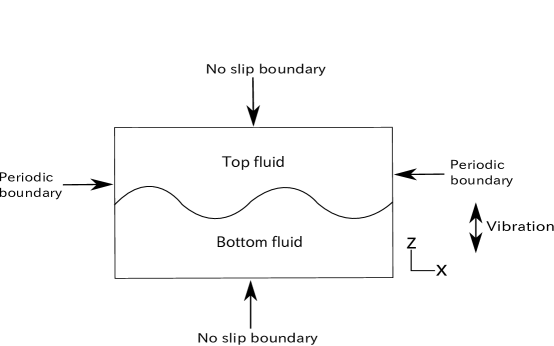
Figure 1: Faraday wave setting in two-dimensional space.

In the horizontal direction (coordinate $x$), we assume periodic boundary conditions with length $L_{x}$. For the vertical direction (coordinate $z$), no-slip boundary conditions at the boundaries $z=0,L_{z}$ are assumed, that is, $\bm{u}(x,0,t)=\bm{u}(x,L_{z},t)=0$. The interface position between the top and bottom fluids, denoted as $z=\zeta(x,t)$, obeys the kinematic boundary condition. In terms of this $\zeta(x,t)$, the density $\rho$ and viscosity $\eta$ in (1) are written as function of $z$:

$$(\rho,\,\eta)=\begin{cases}(\rho_{\rm t},\,\eta_{\rm t})&z>\zeta(x,t),\\ (\rho_{\rm b},\,\eta_{\rm b})&z\leq\zeta(x,t).\end{cases}$$ (4)

In this sharp interface formulation, the density and viscosity vary discontinuously as a function of $z$, which makes numerical simulations in this form very difficult in practice. One standard way to overcome this in numerical simulations is to model the sharp interface by a diffuse one (Anderson, McFadden & Wheeler, 1998). The phase-field modelling is one such diffuse-interface method, which we will explain below.

We adapt the phase-field modelling of binary fluids (Jacqmin, 1999) to Faraday waves. The top and bottom fluids are here indicated by the phase variable values $\phi=1$ and $\phi=-1$, respectively. The interface is modelled as the region where $\phi$ changes continuously from $-1$ to $1$. The phase evolves to minimize the free energy functional of the phase $\phi$:

$$F[\phi(\bm{x},t)]=\frac{\Lambda}{2}\int\left[\frac{1}{2\epsilon^{2}}(\phi^{2}-1)^{2}+|\boldsymbol{\nabla}\phi|^{2}\right]d\bm{x}.$$ (5)

Accordingly, the equation of the phase variable is the Cahn-Hilliard equation with the advection term

$$\frac{\partial\phi}{\partial t}+\bm{u}\boldsymbol{\cdot}\boldsymbol{\nabla}\phi=\gamma\boldsymbol{\nabla}^{2}\mu,$$ (6)

$$\mu=\frac{\delta F}{\delta\phi}=\Lambda\left(-\boldsymbol{\nabla}^{2}\phi+\frac{\phi^{3}-\phi}{\epsilon^{2}}\right).$$ (7)

where $\mu$ is the chemical potential, $\Lambda$ is the magnitude of the free energy and $\gamma$ is the mobility. We assume that the mobility $\gamma$ is constant. The parameter $\epsilon$ controls the thickness of the smoothed interface. These $\gamma$ and $\epsilon$ are adjustable parameters of the phase-field modelling. How to determine them is discussed at the end of section 3. In terms of $\phi$, the density and viscosity are expressed as

$$\rho=\frac{\rho_{\rm t}+\rho_{\rm b}}{2}+\frac{\rho_{\rm t}-\rho_{\rm b}}{2}\phi,\qquad\eta=\frac{\eta_{\rm t}+\eta_{\rm b}}{2}+\frac{\eta_{\rm t}-\eta_{\rm b}}{2}\phi.$$ (8)

In the framework of the phase-field modelling, the surface tension force written as $\bm{s}$ in (1) is given by

$$\bm{s}=\mu\boldsymbol{\nabla}\phi$$ (9)

(Jacqmin, 1999; Celani, Mazzino, Muratore-Ginanneschi & Vozella, 2009). The surface tension $\sigma$ used in the sharp interface model is related to the phase-field simulation parameters as

$$\sigma=\frac{2\sqrt{2}}{3}\frac{\Lambda}{\epsilon}$$ (10)

for planar interfaces. In the following we assume that the correspondence (10) is valid for non-planar interfaces. We use the following boundary conditions of the phase variable on the top and bottom walls $z=0,L_{z}$:

$$\bm{e}_{z}\boldsymbol{\cdot}\boldsymbol{\nabla}\phi=0,\qquad\bm{e}_{z}\boldsymbol{\cdot}\boldsymbol{\nabla}\mu=0$$ (11)

(Jacqmin, 1999). In the horizontal direction, the boundary condition is periodic. For further details of the derivation of the phase-field model, we refer the reader to Jacqmin (1999).

To summarise this subsection, the equations to be solved numerically are the incompressible Navier-Stokes equations (1) and (2) and the Cahn-Hilliard equation (6). The boundary conditions on the velocity are periodic in the horizontal direction and no-slip on the top and bottom walls in the two-dimensional space. For the phase variable, the boundary conditions are periodic in the $x$-direction and (11) in the $z$-direction.

2.2 Numerical method

We start with the discretization of the Cahn-Hilliard equation. The computational mesh is a standard staggered arrangement as in Périnet, Juric & Tuckerman (2009). We Fourier-expand the phase variable $\phi$ in the periodic $x$-direction as

$$\phi(x,z,t)=\sum_{j}\hat{\phi}(k,z,t)~{}{\rm e}^{{\rm i}k_{j}x}.$$ (12)

The wavenumber is given by $k_{j}=(2\pi/L_{x})j\quad(j=-N_{x}/2+1,...,N_{x}/2)$ , where $N_{x}$ is the number of grid points in the $x$-coordinate. Then the Cahn-Hilliard equation in the $(k,z)$ space becomes

$$\frac{\partial\hat{\phi}}{\partial t}+\widehat{(\bm{u}\!\boldsymbol{\cdot}\!\boldsymbol{\nabla})\phi}=\gamma\Lambda\left\{-\left(-k^{2}+\frac{\partial^{2}}{\partial z^{2}}\right)^{2}\hat{\phi}-\frac{1}{\epsilon^{2}}\left[\left(-k^{2}+\frac{\partial^{2}}{\partial z^{2}}\right)\left(\hat{\phi}-\widehat{\phi^{3}}\right)\right]\right\},$$ (13)

where the cubic term $\widehat{\phi^{3}}$ is the Fourier transform of the product $\phi^{3}$ calculated in the physical space $(x,z)$. No aliasing error is removed in this calculation of $\widehat{\phi^{3}}$.

The advection term $\widehat{(\bm{u}\boldsymbol{\cdot}\boldsymbol{\nabla})\phi}$ is calculated as follows. First it is calculated in the physical space by using an elementary discretization in the staggered mesh as

$$\left[(\bm{u}\boldsymbol{\cdot}\boldsymbol{\nabla})\phi\right]_{l,\,m}=\left(u\frac{\partial\phi}{\partial x}+w\frac{\partial\phi}{\partial z}\right)_{l,\,m}$$

$$=\frac{u_{l-1/2,\,m}+u_{l+1/2,\,m}}{2}\,\,\frac{\phi_{l+1,\,m}-\phi_{l-1,\,m}}{2\Delta x}+\frac{w_{l,\,m-1/2}+w_{l,\,m+1/2}}{2}\,\,\frac{\phi_{l,\,m+1}-\phi_{l,\,m-1}}{2\Delta z}$$

. (14)

In this notation $u_{l-1/2,\,m}$ denotes the velocity on the cell face $(x_{l-1/2},z_{m})$ and $\phi_{l,m}$ denote the phase variable on the cell centre $(x_{l},z_{m})$. The indices run as $l=1,\cdots,N_{x}$ and $m=1,\cdots,N_{z}$ ($N_{z}$ is the number of grid points on the $z$-coordinates). In the denominator $\Delta x$ and $\Delta z$ are the grid spacings of the $x$ and $z$ coordinates. The Fourier transform of (14) gives $\widehat{(\bm{u}\boldsymbol{\cdot}\boldsymbol{\nabla})\phi}$. Again no aliasing error is removed.

Equation (13) is discretized in time by using the semi-implicit stabilized scheme due to Eyre (1997) as

$$\frac{\hat{\phi}^{(n+1)}-\hat{\phi}^{(n)}}{\Delta t}+\widehat{(\bm{u}^{(n)}\boldsymbol{\cdot}\boldsymbol{\nabla})\phi^{(n)}}$$

$$=\gamma\Lambda\left\{-\left(-k^{2}+\frac{\partial^{2}}{\partial z^{2}}\right)^{2}\hat{\phi}^{(n+1)}-\frac{1}{\epsilon^{2}}\left[\left(-k^{2}+\frac{\partial^{2}}{\partial z^{2}}\right)\left(3\hat{\phi}^{(n)}-2\hat{\phi}^{(n+1)}-\widehat{(\phi^{(n)})^{3}}\right)\right]\right\}.$$

(15)

Here $\hat{\phi}^{(i)}$ denotes the data at the $i$-th time step. On the right hand side, the fourth-order derivative term is treated fully implicitly. The second-order term is handled semi-implicitly, which is split into two terms: one involves $3\hat{\phi}^{(n)}$ and the other $2\hat{\phi}^{(n+1)}$ as proposed by Eyre (1997). The $z$-derivatives in (15) are evaluated as

$$\left(\frac{\partial^{2}\hat{\phi}}{\partial z^{2}}\right)_{j,m} = \frac{1}{\Delta z^{2}}\left(\hat{\phi}_{j,m+1}-2\hat{\phi}_{j,m}+\hat{\phi}_{j,m-1}\right),$$ (16)

$$\left(\frac{\partial^{4}\hat{\phi}}{\partial z^{4}}\right)_{j,m} = \frac{1}{\Delta z^{4}}\left(\hat{\phi}_{j,m+2}-4\hat{\phi}_{j,m+1}+6\hat{\phi}_{j,m}-4\hat{\phi}_{j,m-1}+\hat{\phi}_{j,m-2}\right),$$ (17)

where $\hat{\phi}_{j,m}$ denotes $\hat{\phi}(k_{j},m\Delta z)$. We use the bi-conjugate gradient stabilized (BiCGSTAB) method (Saad, 1996) to solve the equations (15). The boundary conditions of $\phi$ in the $z$-direction are given in (11).

Now we turn to discretization of the incompressible Navier-Stokes equations (1) and (2). We follow mostly the discretization method proposed by Périnet, Juric & Tuckerman (2009) except for the surface tension force. In order to describe how we calculate the surface tension force in the present phase-field modelling, we repeat here some of the equations given in §3.3 of Périnet, Juric & Tuckerman (2009). The method starts with the intermediate velocity $\tilde{\bm{u}}$ from $\bm{u}^{(n)}$ at the $n$-th time step,

$$\frac{\tilde{\bm{u}}-\bm{u}^{(n)}}{\Delta t}=-(\bm{u}^{(n)}\boldsymbol{\cdot}\boldsymbol{\nabla})\bm{u}^{(n)}+\frac{1}{\rho^{(n+1)}}\boldsymbol{\nabla}\boldsymbol{\cdot}\eta^{(n+1)}(\boldsymbol{\nabla}\tilde{\bm{u}}+\boldsymbol{\nabla}\tilde{\bm{u}}^{T}),$$ (18)

where $\rho^{(n)}$ and $\eta^{(n)}$ are here determined by the phase $\phi^{(n)}$ as (8). Yet another intermediate velocity $\bm{u}^{*}$ involves the gravity and the vibration forces $\bm{G}$ and the surface tension force $\bm{s}$:

$$\frac{\bm{u}^{*}-\tilde{\bm{u}}}{\Delta t}=\bm{G}^{(n+1)}+\frac{\bm{s}^{(n+1)}}{\rho^{(n+1)}}-\frac{1}{\rho^{(n+1)}}\boldsymbol{\nabla}p^{(n)}.$$ (19)

Since this $\bm{s}$ is represented as (9) in the phase-field method, we discretize each component first as

$$\left(s_{x}\right)^{(n)}_{l,m}= \mu_{l,m}^{(n)}\frac{\phi^{(n)}_{l+1,m}-\phi^{(n)}_{l-1,m}}{2\Delta x},\quad\left(s_{z}\right)^{(n)}_{l,m}=\mu_{l,m}^{(n)}\frac{\phi^{(n)}_{l,m+1}-\phi^{(n)}_{l,m-1}}{2\Delta z}.$$ (20)

Then, the vectors $\bm{s}$ on the staggered grids are

$$\left(s_{x}\right)^{(n)}_{l+1/2,m}= \frac{\left(s_{x}\right)^{(n)}_{l+1,m}+\left(s_{x}\right)^{(n)}_{l,m}}{2},\quad\left(s_{z}\right)^{(n)}_{l,m+1/2}=\frac{\left(s_{z}\right)^{(n)}_{l,m+1}+\left(s_{z}\right)^{(n)}_{l,m}}{2}.$$ (21)

Here the chemical potential (7) is discretized as

$$\mu^{(n)}_{l,m} = \Lambda\left[-\frac{\phi^{(n)}_{l+1,m}-2\phi^{(n)}_{l,m}+\phi^{(n)}_{l-1,m}}{\Delta x^{2}}-\frac{\phi^{(n)}_{l,m+1}-2\phi^{(n)}_{l,m}+\phi^{(n)}_{l,m-1}}{\Delta z^{2}}+\frac{(\phi^{(n)}_{l,m})^{3}-\phi^{(n)}_{l,m}}{\epsilon^{2}}\right].$$

Finally, the velocity at the $(n+1)$-th time step is obtained by

$$\frac{\bm{u}^{(n+1)}-\bm{u}^{*}}{\Delta t}=-\frac{1}{\rho^{(n+1)}}\boldsymbol{\nabla}\left(p^{(n+1)}-p^{(n)}\right),$$ (23)

where the pressure $p^{(n+1)}$ is determined, by demanding $\boldsymbol{\nabla}\boldsymbol{\cdot}\bm{u}^{(n+1)}=0$, as

$$\frac{\boldsymbol{\nabla}\boldsymbol{\cdot}\bm{u}^{*}}{\Delta t}=\boldsymbol{\nabla}\boldsymbol{\cdot}\frac{1}{\rho^{(n+1)}}\boldsymbol{\nabla}\left(p^{(n+1)}-p^{(n)}\right).$$ (24)

Again the BiCGSTAB method is employed to solve (18) and (24). The boundary conditions for the velocity and the intermediate one $\tilde{\bm{u}}$ are the same as in Périnet, Juric & Tuckerman (2009), namely, $\tilde{\bm{u}}(x,z=0\,{\rm or}\,L_{z},t)=0$, $\bm{e}_{z}\boldsymbol{\cdot}\bm{u}^{(n+1)}(x,z=0\,{\rm or}\,L_{z},t)=0$ and $\bm{e}_{z}\boldsymbol{\cdot}\nabla[p^{(n+1)}(x,z=0\,{\rm or}\,L_{z},t)-p^{(n)}(x,z=0\,{\rm or}\,L_{z},t)]=0$. As proposed by Périnet, Juric & Tuckerman (2009), in solving the equations (18), we use the latest updated velocity component of $\tilde{\bm{u}}$ to compute the other component. In this process, the order (which component of $\tilde{\bm{u}}$ is computed first and last) is also interchanged at each time step to ensure symmetry.

3 Comparison in the linear regime

We compare our simulation result with the linear theory of Kumar & Tuckerman (1994). We follow here again the validation method proposed by Périnet, Juric & Tuckerman (2009).

In the linear theory elaborated by Kumar & Tuckerman (1994), the Faraday wave problem is formulated as a finite-depth, viscous binary fluid system with a sharp interface representation. This provides the critical value of the vibration forcing amplitude $a_{c}$ as eigenvalues for a given perturbation ${\rm e}^{{\rm i}kx}$. The Floquet modes $f_{q}(k)$ of the interface position $z=\zeta(x,t)$ can be calculated as eigenvectors. In other words, the spatio-temporal variation reads(Kumar & Tuckerman, 1994)

$$\zeta(x,t)\propto{\rm e}^{{\rm i}kx}~{}{\rm e}^{(\beta+{\rm i}\alpha\omega)t}\sum_{q=-N_{\rm F}}^{N_{\rm F}}f_{q}(k)~{}{\rm e}^{{\rm i}q\omega t}.$$ (25)

Recall that $\omega$ is the angular frequency of the vibration forcing (3). Here the number of Floquet modes $N_{\rm F}$ is infinite in theory but it is finite for numerical calculations. The exponent $\beta+{\rm i}\alpha\omega$ is the Floquet exponent. For the critical perturbations $\beta$ is zero. The harmonic $\alpha=0$ and subharmonic $\alpha=1/2$ cases are considered here as in Périnet, Juric & Tuckerman (2009).

Figure 2: Critical curve of the vibration amplitude from the linear theory (Kumar & Tuckerman, 1994). Points are the critical values determined with the phase-field simulation.

We numerically solve this eigenvalue problem (for the precise form of the matrices, see Kumar & Tuckerman (1994)). The Mathematica script that we use here is available at http://www.kyoryu.scphys.kyoto-u.ac.jp/~takeshi/kt94. The parameters here are the same as in Périnet, Juric & Tuckerman (2009) in their validation with the linear theory. The parameter values are $N_{F}=10$, $\rho_{\rm b}=5.19933\times 10^{2}$ kg m^-3, $\rho_{\rm t}=4.15667\times 10^{2}$ kg m^-3, $\eta_{\rm b}=3.908\times 10^{-5}$ Pa s, $\eta_{\rm t}=3.124\times 10^{-5}$ Pa s, $\sigma=2.181\times 10^{-6}$ N m^-1, $g=9.8066$ m s^-2, $L_{z}=2.31\times 10^{-4}$ m and $\omega=2\pi\times 10^{2}$ s^-1. The unperturbed interface is in the centre of the container. The critical vibration forcing amplitude $a_{c}$ from the linear theory as a function of the perturbation wavenumber $k$ is plotted as a curve in figure 2. The Floquet modes $f_{q}$ are used later in figure 3.

With the phase-field simulation, critical values $a_{c}$ for four different $k$’s are determined, which are denoted as points in figure 2. Refer also to table 1 for a precise comparison with the values from the linear theory calculation. We see that agreement between the two is satisfactory.

The way to estimate $a_{c}$ in the phase-field simulation is as follows. (i) We consider the sharp interface location $z=\zeta(x,t)$ in the linear analysis to be the null point $\phi=0$ in the phase-field modelling. Numerically, such null points are calculated using the linear interpolation of $\phi$ data on the grid points (we use this correspondence throughout this paper). (ii) For a given acceleration amplitude $a$, we monitor the oscillating interface position at $x=L_{x}/2$ as a function of time. We perform simulations by changing $a$ from the theoretical $a_{c}$ and estimate the critical value at which the temporal oscillation neither decays nor grows. More precisely, we take the absolute relative difference between the two peak values of the interface positions around $t=2T_{\rm v}$ and $4T_{\rm v}$. If the difference is smaller than $10^{-3}$, we regard this $a$ as the critical acceleration of the phase-field simulation. The largest error shown in table 1 (the case of $k=28.0$) would be due to a relatively large $\Delta x=L_{x}/N_{x}$.

Here we set the parameters of the phase-field simulation to be $\epsilon=\Delta z=1.80\times 10^{-6}$ m, $\gamma=6.33\times 10^{-8}\,{\rm m^{3}kg^{-1}s}$, $\Lambda=3\sigma/(2\sqrt{2}\epsilon)$ (see (10)) and $\Delta t=2.5\times 10^{-6}$ for all four cases. The initial perturbed interface is written in terms of the phase variable as

$$\phi=\tanh\left\{\frac{z-[L_{z}/2-b\cos(kx)]}{\sqrt{2}\epsilon}\right\},$$ (26)

where $b$ corresponds to the perturbation amplitude of the interface position. Here we take $b=3\Delta z=3\epsilon$. We recall that in the unperturbed state the Cahn-Hilliard equation has the stationary solution $\phi(z)=\tanh[(z-L_{z}/2)/(\sqrt{2}\epsilon)]$ (see, e.g. Jacqmin (1999)). The initial velocity in the phase-field simulation is set to zero.

$k\,({\rm mm}^{-1})$	$L_{x}({\rm mm})$	$a_{c}/g$ (theory)	$a_{c}/g$ (simu.)	error$\,(\%)$
28.0	0.224	4.37	4.65	6.0
48.0	0.131	12.5	12.5	0.0
73.0	0.0861	28.5	28.4	0.49
94.0	0.0668	51.0	50.0	2.0

Table 1: Critical amplitude values $a_{c}$ of the linear theory calculation and the phase-field simulation. Here the horizontal length of the simulation $L_{x}$ is taken to be equal to the wavelength of the perturbation $2\pi/k$ for every case. The number of grid points of the simulation is $N_{x}\times N_{z}=128\times 128$

.

Figure 3 shows temporal variations of the interface location obtained by the Floquet analysis results (25) and the phase-field simulation results with critical $a_{c}$ values. We here follow the representation used in Périnet, Juric & Tuckerman (2009). The initial discrepancies between the linear theory and the simulation remain large until one vibrating period $T_{\rm v}$. However, later than that, the phase-field solutions agree satisfactorily with the Floquet analysis result as shown in figure 3. In contrast, the discrepancies between the simulation by Périnet, Juric & Tuckerman (2009) and the linear theory vanish within a quarter of the period of the vibration.

Figure 3: Time variations of the interface position at $x=L_{x}/2$ of the phase-field simulation (circles) and the Floquet analysis result (curves). The interface position is defined as the phase null points $\phi=0$. The thick arrows indicate the size of $\epsilon$, which is the length scale of the diffuse interface. (a) Perturbation wavenumber $k=48.0$ mm^-1 (subharmonic case); (b) $k=73.0$ mm^-1 (harmonic case); (c) $k=94.0$ mm^-1 (subharmonic case).

Finally, we comment on the values of the mobility $\gamma$ and the thickness of the interface $\epsilon$, which are adjustable numerical parameters of the phase-field simulation. The mobility $\gamma$ is determined as follows. The physical time scales of the various forces in (1) can be dimensionally estimated for a given length scale $l_{0}$ as $t_{g}=(l_{0}/g)^{1/2},\,t_{\eta}=l_{0}^{2}\rho/\eta$ and $t_{\sigma}=(l_{0}^{3}\rho/\sigma)^{1/2}$, which are times scales of the gravity, viscosity and surface tension, respectively. The time scale associated with the mobility is in a similar way given as $t_{\gamma}=\gamma\rho$ by (6). The mobility value is determined by requiring $t_{\gamma}<\min\{t_{g},t_{\eta},t_{\sigma}\}$ for a small length scale, say $l_{0}=\epsilon$. This means that the interface’s relaxation to equilibrium occurs faster than other dynamics. Here we have $t_{g}=4.29\times 10^{-4},t_{\eta}=3.47\times 10^{-5}$ and $t_{\sigma}=3.34\times 10^{-5}$s. To have the condition $t_{\gamma}<\min\{t_{g},t_{\eta},t_{\sigma}\}$, we set $\gamma=6.33\times 10^{-8}$ kg^-1m³s, which yields $t_{\gamma}=2.63\times 10^{-5}$s. That is, $t_{\gamma}/\min\{t_{g},t_{\eta},t_{\sigma}\}=0.79$ here. If this ratio is larger than $1.0$, our simulation does not agree with the linear theory. Here we take the time step to be $\Delta t=2.50\times 10^{-6}$s, which is about an order of magnitude smaller than $t_{\gamma}$. The thickness $\epsilon$ is determined as follows. We first fix the perturbation amplitude to $b=3\Delta z$ and then do simulations with $\epsilon/\Delta z=0.5,1.0,2.0,...,5.0$. Good agreement with the $a_{c}$ of linear theory is obtained for $\epsilon/\Delta z\leq 3.0$. This leads us to choose $\epsilon=\Delta z$.

4 Simulation beyond the linear regime

Having validated the phase-field approach in the linear regime, we now move to nonlinear regimes. Two cases are considered. The first one concerns plume formation, which may eventually lead to droplet ejection at long time. However, we do not follow the motion until the ejection or pinchoff occurs. The second case is the period tripling state of the two-dimensional Faraday waves.

4.1 Plume formation

Plume formation of the Faraday interfaces in two dimensions was studied numerically by Wright, Yon & Pozrikidis (2000) using the vortex-sheet method, with which we compare the phase-field simulation. The presence of a plume implies that the interface profile becomes a multivalued function of the horizontal coordinate. Such situations can be numerically handled by the phase-field method without ad hoc adjustments.

Here the comparison is qualitative. There are three reasons for this: the difference in Atwood number $A={(\rho_{\rm b}-\rho_{\rm t})}/{(\rho_{\rm b}+\rho_{\rm t})}$, the difference in the boundary conditions, and with or without viscosity. Regarding the Atwood number difference, the phase-field method with the discretization described in section 2.2 is not able to handle high Atwood number $A$. Our simulation works for at most $A\simeq 0.40$ in practice (this issue is discussed in the last §5). In contrast, the vortex-sheet calculation by Wright, Yon & Pozrikidis (2000) can cope with up to unit Atwood number. Concerning the difference in the boundary conditions, there is no rigid boundary in the vertical direction in their vortex-sheet calculation. However, in our case fluids are contained between two rigid walls. The third reason is that the vortex-sheet calculation is inviscid, while the phase-field method is viscous.

In Wright, Yon & Pozrikidis (2000), the overturning interface corresponding to formation of a plume at $A=0.65$ and $1.0$ is numerically studied. We observe a similar overturning behaviour in the phase-field simulation even at as low as $A=0.10$, which we show in figure 4. The parameters of the phase simulation are: $L_{x}=1.0{\rm m},L_{z}=1.0{\rm m},a=9.0\times 10^{-2}{\rm ms^{-2}},\omega=2.6728\times 10^{-1}{\rm s^{-1}},\rho_{\rm b}=1.0\times 10^{3}{\rm kgm^{-3}},\rho_{\rm t}=8.1818\times 10^{2}{\rm kgm^{-3}},\eta_{\rm t}=0.2{\rm Pas},\eta_{\rm b}=0.2{\rm Pas},\sigma=7.2\times 10^{-2}{\rm Nm^{-1}},g=0.0,$ $\Lambda=3\sigma/(2\sqrt{2}\epsilon),\gamma=5.61\times 10^{-4}{\rm m^{3}kg^{-1}s}$ and $\epsilon=\Delta z$. The force $\bm{G}$ in (1) is here $\bm{G}=a\cos\omega t$, oscillating around zero. The initial interface is given by (26) with $b=0.01{\rm m}$. The time step and the number of grid points are $\Delta t=1.18\times 10^{-3}$ and $N_{x}\times N_{z}=256\times 256$. Here we take the same parameters $L_{x},\omega,\rho_{\rm b},b,\sigma$ and the same vibration force $\bm{G}$ setting (oscillating around the origin) as Wright, Yon & Pozrikidis (2000). The differences between our simulations and theirs are the Atwood number, the vibration amplitude value (ours are nine times larger), the presence of the top and bottom rigid walls and the presence of viscosity.

The time variation of the interface location at a fixed horizontal point is shown in figure 4(a). The interface location first exhibits a rise and then a fall (here at about $1.5T_{\rm v}$ and $2.5T_{\rm v}$, respectively, where $T_{\rm v}$ is the vibration period); then it grows steeply (at around $t=3.0T_{\rm v}$) and reaches a high plateau (between $t=3.4T_{\rm v}$ and $t=4.4T_{\rm v}$) with a small oscillation. This variation is similar to that with $A=0.65$ obtained with the vortex-sheet method (figure 11(a) of Wright, Yon & Pozrikidis (2000)). In our simulation, the interface location later than $t=5T_{\rm v}$ (continuation of figure4(a) but not shown) goes downwards and shows again a plateau with a small oscillation. Then it goes upwards and finally comes back to zero around $t=8T_{\rm v}$. This later variation cannot be compared with the vortex-sheet method result of Wright, Yon & Pozrikidis (2000) because their calculation is stopped before $t=5T_{\rm v}$.

The phase field $\phi$ at $t=3.5T_{\rm v}$ is shown in figure 4(b), which clearly shows that the interface turns over and becomes a multivalued function of the horizontal coordinate $x$. Qualitatively similar interface structures, called plumes, are shown in figure 11(b) of Wright, Yon & Pozrikidis (2000). To check the boundary effect, we also do the phase-field simulation with aspect ratio 2 ($L_{x}=2L_{z}$). The plume shape and its time evolution do not change qualitatively, indicating that the effect of the vertical boundary is small on the plume formation. This agreement suggests that the phase-field simulation is valid, at least qualitatively, in the overturning regime although it cannot handle cases with high Atwood number.

In figure 4(c) and (e), we plot the vorticity field $\Omega=\partial_{z}u-\partial_{x}w$ at the plume state. Indeed much of the vorticity concentrates inside the interface region. The vorticity along the interface in the right half domain has three peaks as seen in the contour plot of figure 4(e). In contrast, in the simulation of Wright, Yon & Pozrikidis (2000), the strength of the vortex sheet has at most two peaks in the developed plume state. In the phase-field simulation we observe that the vorticity outside of the interface reaches about 40% of the maximum vorticity in the interface region. In addition, thin vortex layers are attached near the top and bottom walls. In these layers, the vorticity is about 10% of the maximum in the interface region.

We now comment on the choice of the resolution $N_{x}\times N_{z}=256\times 256$ used here. We observe that the squared modulus of the Fourier coefficients $|\hat{\phi}(k,z,t)|^{2}$ decreases exponentially for large $k$ such as $|\hat{\phi}(k,z,t)|^{2}\propto\exp[-\delta(z,t)k]$. We measure this factor $\delta(z,t)$ and require $\max_{z,t}[\delta(z,t)]\geq 2\Delta x=2L_{x}/N_{x}$. We take the smallest $N_{x}$ in powers of 2 satisfying this relation. We then set $\Delta z$ to about the same value of $\Delta x$.

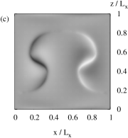
Figure 4: Faraday interface in a nonlinear regime, showing an overturning behaviour in the phase-field simulation. (a) Time variation of the interface position at $x=L_{x}/2$. The interface position is defined from the phase field $\phi$ as described in section 3. (b) Grey-scale coded phase field $\phi$ at time $t=3.5T_{\rm v}$. (c) Grey-scale coded vorticity field at the same instant. (d) Interface profiles at four instants. (e) Contours of the vorticity at $t=3.5T_{\rm v}$. Contour values are from -20.0 to 20.0 by 4.0. The solid and dashed lines correspond to non-negative and negative vorticity values.

4.2 Period tripling

The period tripling state of Faraday waves, in which the period of the standing wave becomes three times the usual subharmonic period (which is in turn twice the vibration period), is found in the quasi-two-dimensional experiment by Jiang, Perlin & Schultz (1998) (see also Perlin & Schultz (2000)) and in the three-dimensional axisymmetric experiment by Jiang, Perlin & Schultz (1998) and also by Das & Hopfinger (2008). In the two-dimensional vortex-sheet simulation of Wright, Yon & Pozrikidis (2000), period tripling is also observed. From their numerical result, Wright, Yon & Pozrikidis (2000) conclude that the period tripling is caused by the nonlinearity of the irrotational flow. We here aim at reproducing the period tripling state with the phase-field modelling within our feasible Atwood number range $A<0.40$, although the above experiments and the vortex-sheet simulation are conducted in the case $A\simeq 1.0$.

By searching the parameter space, which will be discussed later, indeed we observe the period tripling state at low Atwood number $A=0.11$, as depicted in figure 5. The interface shapes at the maxima are shown in figure 6, some of which actually differ from the previous observations. In the experiment by Jiang, Perlin & Schultz (1998), the interface shapes at the three peaks in the tripling state are classified as sharp crest (called mode A by them), flat or dimpled crest (mode B) and round crest (mode C), respectively. The corresponding shapes of the phase-field simulation shown in figure 6(a–c) are qualitatively different except for the round crest (figure 6(c)). In particular, the hourglass plume shown in figure 6(a) and waistless plume in figure 6(b) are different from the sharp crest (mode A) and the flat or dimpled crest (mode B). These sharp and flat crests are associated with wave breaking in Jiang, Perlin & Schultz (1998) but not necessarily so in Das & Hopfinger (2008). In the phase-field simulation with this parameter set, wave breaking does not occur. In the period tripling state observed numerically by Wright, Yon & Pozrikidis (2000), plume-type interfaces are not observed.

The vorticity contours at the three peaks are shown in figure 6(d–f). The number of vortex peaks inside the interface region is three for the hourglass plume and one for the waistless plume and the round crest. Outside of the interface region the vorticity is weaker but not zero.

To find the parameters of the period tripling state in practice, we use as a guide the phase diagram made by Jiang, Perlin & Schultz (1998) in the space of the detuning parameter $p$ and forcing parameter $q$. We search this $p,q$-space horizontally (constant $p$) by going away from the neutral curve as shown in figure 7. We take seven parameter sets along this line. The period tripling state is found at the middle point. In the phase diagram in Jiang, Perlin & Schultz (1998), the period tripling state extends for the large $q$ region. But our case is very different. The parameters of the tripling state are: $L_{x}=1.46\times 10^{-4}$ m, $L_{z}=2.31\times 10^{-4}$ m, $a/g=9.5$, $\omega=2\pi\times 10^{2}$ s^-1, $\rho_{\rm b}=5.19933\times 10^{2}$ kg m^-3, $\rho_{\rm t}=4.15667\times 10^{2}$ kg m^-3, $\eta_{\rm b}=3.908\times 10^{-5}$ Pa s, $\eta_{\rm t}=3.124\times 10^{-5}$ Pa s, $\sigma=2.181\times 10^{-6}$ N m^-1, $g=9.8066$ m s^-2, $\epsilon=\Delta z=1.80\times 10^{-5}$ m, $\gamma=6.33\times 10^{-8}\,{\rm m^{3}kg^{-1}s}$, $\Lambda=3\sigma/(2\sqrt{2}\epsilon)$ and $N_{x}\times N_{z}=128\times 128$. The spatial resolution is determined in the same way as described in subsection 4.1.

Now we discuss the behaviours at other parameter points shown in figure 7. For three $q$ values smaller than the period tripling value, we observe that the period of the standing wave remains twice the vibration period (the subharmonic period). The interface shape at the maximum and minimum surface elevations are hourglass-plume type. In other words, the temporal symmetry is kept as we approach the period tripling state from the left while in the experiment and numerical simulation by Jiang, Ting, Perlin & Schultz (1996) the symmetry is broken before reaching the tripling state. This discrepancy may be due to the difference in the Atwood number or the difference in the dissipation caused by the sidewalls. For the next larger $q$ parameter than that of the tripling state, we observe that the period of the standing wave returns to the subharmonic period ($2T_{\rm v}$). We do not have an explanation for this. The interface shape at the maximum and minimum elevation is also of the hourglass-plume type. For the two largest $q$ parameters that we calculate, the oscillation becomes close to quasi-periodic. The interface shapes at relative maximum elevations in this parameter range take the three forms shown in figure 6(a-c) almost randomly.

Figure 5: Temporal variation of the interface position at $x=L_{x}/2$, showing the period tripling. Here $T_{\rm v}$ is the period of the vibration forcing.

Figure 6: Interface profiles corresponding to the three peaks of the period tripling state (a) $t=19.4T_{\rm v}$; (b) $t=21.4T_{\rm v}$; (c) $t=23.4T_{\rm v}$. They correspond to the last three peaks shown in figure 5. Vorticity contours (solid and dotted lines correspond to non-negative and negative values, respectively) at the same instances: (d) $t=19.4T_{\rm v}$, the contour values are from $-5.0$ to $5.0$ by $1.0$; (e) $t=21.4T_{\rm v}$, the values are from $-7.0$ to $7.0$ by $1.0$; (f) $t=23.4T_{\rm v}$, the values are the same as (e).

Figure 7: The $p,q$ parameter space for seeking the period tripling regime. Here $p=\{2\Omega(k)/\omega\}^{2}$ is the detuning parameter and $q=2Aka/\omega^{2}$ is the forcing parameter, where $\Omega^{2}(k)=kg[A+\sigma k^{2}/\{g(\rho_{\rm b}+\rho_{\rm t})\}]$. The points are $q=2.00,\,2.11,\,2.17,\,2.23,\,2.29,\,2.35,\,2.41$ and constant $p=2.35$. The curve corresponds to the neutral stability line obtained by the linear analysis of Kumar & Tuckerman (1994) (the method described in §3 is used).

5 Discussion and concluding remarks

We have applied the phase-field modelling of the binary fluids with the Cahn-Hilliard equation due to Jacqmin (1999) to numerical simulations of the Faraday wave problem in two spatial dimensions. Here we have solved the Navier-Stokes equations for both the top and bottom fluids with rigid boundary conditions on the top and bottom walls and with periodic boundary condition for the side walls. Validation of this phase-field simulation is checked quantitatively in the linear regime and qualitatively in the nonlinear regime.

In the linear regime, our simulation agrees quantitatively well with the Floquet analysis by Kumar & Tuckerman (1994) in three different branches, which is the benchmark test proposed in Périnet, Juric & Tuckerman (2009) for the Faraday waves.

In the nonlinear regime, we are not able to validate the present simulation against experimental results unlike Périnet, Juric & Tuckerman (2009). Nevertheless we have considered two cases. Both cases involve plume formation where the two-fluid interface becomes a multivalued function of a horizontal coordinate. Such situations can be a good testing ground for the phase-field method since the method does not break down when the interface turns over.

The nonlinear case we considered first is the bursting plume formation which was studied by Wright, Yon & Pozrikidis (2000) with the vortex-sheet method. Their system setting (the boundary conditions, the dissipation and close-to-unity Atwood number, especially) is very different from the present binary fluid setting. Consequently the comparison is necessarily qualitative. The phase-field method with the numerical scheme described in section 3 works only in the Atwood number range $A<0.40$. Nevertheless we found for very low Atwood number $A=0.10$ that a similar plume is formed and the temporal variation of the interface agrees qualitatively with that in Wright, Yon & Pozrikidis (2000).

The second nonlinear case is the period tripling of the two-dimensional Faraday waves first found experimentally by Jiang, Perlin & Schultz (1998) and numerically by Wright, Yon & Pozrikidis (2000). Again, in spite of the rather big system differences with these studies, we have observed the period tripling state in the phase-field simulation with low Atwood number $A=0.11$. This result adds further evidence for the robustness of the period tripling as discussed in Jiang, Perlin & Schultz (1998). More detailed numerical study of the tripling state is currently under way and will be reported elsewhere. It would be interesting to perform a laboratory experiment with the same physical parameters as in §4.2 to check whether or not the period tripling is observed.

Concerning the limitation on the Atwood number $A<0.40$ in the present phase-field simulation, we do not have an explanation for why it is so. For $A\geq 0.40$, we observe that, if we put a larger number of grid points inside the interface region, we can postpone the breakdown of the simulation until somewhat later (we can continue the simulation for a larger number of time steps). However, increasing the number of grid points there may cause a new problem. Although Jacqmin (2000) successfully reaches Atwood number $0.98$, he reports that the interface becomes much wider than in reality. It is not clear to us for the present whether or not we can overcome these problems by improving the temporal and spatial discretizations of the Cahn-Hilliard and Navier-Stokes equations.

Finally, we comment on extension of the phase-field method to three-dimensional Faraday waves. It is straightforward. We believe that the three-dimensional phase-field method, once extended, can be complementary to the simulation method by Périnet, Juric & Tuckerman (2009) since the two methods are different. There is an interesting instance of three-dimensional Faraday waves, where the interface becomes multivalued. That is the propagating solitary state observed by Lioubashevski, Arbell & Fineberg (1996). Our simulation code can easily study such a state.

We acknowledge the support by the Grant-in-Aid for the Global COE Program ”The Next Generation of Physics, Spun from Universality and Emergence” from the MEXT of Japan and by the Grant-in-Aid for Young Scientists (B) No. 2174290 from the JSPS. We thank the anonymous referees for constructive criticisms.

References

- Anderson, McFadden & Wheeler (1998) Anderson, D. M., McFadden, G. B. & Wheeler, A. A. 2000 Diffuse-interface methods in fluid mechanics. Ann. Rev. Fluid Mech. 30, 139–165.
- Arbell & Fineberg (2000) Arbell, H. & Fineberg, J. 1999 Temporally harmonic oscillons in Newtonian fluids. Phys. Rev. Lett. 85, 756–759
- Celani, Mazzino, Muratore-Ginanneschi & Vozella (2009) Celani, A., Mazzino, A., Muratore-Ginanneschi, P. & Vozella, L. 2009 Phase-field model for the Rayleigh-Taylor instability of immiscible fluids. J. Fluid Mech. 622, 115–134.
- Chen & Viñals (1999) Chen, P. & Viñals, J. 1999 Amplitude equation and pattern selection in Faraday waves. Phys. Rev. E. 60, 559–570.
- Chen & Wu (2000) Chen, P. & Wu, K. 2000 Subcritical bifurcations and nonlinear balloons in Faraday waves. Phys. Rev. Lett. 85, 3813–3816.
- Das & Hopfinger (2008) Das, S. P. & Hopfinger, E. J. 2008 Parametrically forced gravity waves in a circular cylinder and finite-time singularity. J. Fluid Mech. 599, 205–228.
- Eyre (1997) Eyre, D. J. 1990 An unconditionally stable one-step scheme for gradient systems. http://www.math.utah.edu/~eyre/research/methods/stable.ps
- Faraday (1831) Faraday, M. 1831 On a peculiar class of acoustical figures; and on certain forms assumed by groups of particles upon vibrating elastic surfaces. Phil. Trans. R. Soc. Lond. 121, 299–340. See also http://openlibrary.org/books/OL6976494M/Experimental_researches_in_chemistry_and_physics, which is a scan of the book: Faraday, M. 1859 Experimental researches in chemistry and physics. R. Taylor and W. Francis, London.
- Jacqmin (1999) Jacqmin, D. 1999 Calculation of two-phase Navier-Stokes flows using phase-field modeling. J. Comput. Phys. 155, 96–127.
- Jacqmin (2000) Jacqmin, D. 2000 Contact-line dynamics of a diffuse fluid interface. J. Fluid Mech. 402, 57–88.
- Jiang, Perlin & Schultz (1998) Jiang, L., Perlin, M. & Schultz, W. W. 1998 Period tripling and energy dissipation of breaking standing waves. J. Fluid Mech. 369, 273–299.
- Jiang, Ting, Perlin & Schultz (1996) Jiang, L., Ting, C., Perlin, M. & Schultz, W. W. 1996 Moderate and steep Faraday waves: instabilities, modulation and temporal asymmetries. J. Fluid Mech. 329, 275–307.
- Kityk, Embs, Mekhonoshin & Wagner (2005) Kityk, A. V., Embs, J., Mekhonoshin, V. V. & Wagner, C. 2005 Spatiotemporal characterization of interfacial Faraday waves by means of a light absorption technique. Phys. Rev. E. 72, 036209.
- Kumar & Tuckerman (1994) Kumar, K. & Tuckerman, L. S. 1994 Parametric instability of the interface between two fluids. J. Fluid Mech. 279, 49–68.
- Lioubashevski, Arbell & Fineberg (1996) Lioubashevski, O., Arbell, H. & Fineberg, J. 1996 Dissipative solitary states in driven surface waves. Phys. Rev. Lett. 76, 3959–3962.
- Miles & Henderson (1990) Miles, J. & Henderson, D. 1990 Parametrically forced surface waves. Ann. Rev. Fluid Mech. 22, 143–165.
- Murakami & Chikano (2001) Murakami, Y. & Chikano, M. 2001 Two-dimensional direct numerical simulation of parametrically excited surface waves in viscous fluid. Phys. Fluids 13, 65–74.
- Perlin & Schultz (2000) Perlin, M. & Schultz, W. W. 2000 Capillary effects on surface waves. Ann. Rev. Fluid Mech. 31, 241–274.
- Périnet, Juric & Tuckerman (2009) Périnet, N., Juric, D. & Tuckerman, L. S. 2009 Numerical simulation of Faraday waves. J. Fluid Mech. 635, 1–26.
- Peskin (1977) Peskin, C. S. 1977 Numerical analysis of blood flow in the heart. J. Comput. Phys. 25, 220–252.
- Pucci, Fort, Ben Armar & Couder (2011) Pucci, G., Fort, E., Ben Amar, M. & Couder, Y. 2011 Mutual adaptation of a Faraday instability pattern with its flexible boundaries in floating fluid drops. Phys. Rev. Lett. 106, 024503.
- Saad (1996) Saad, Y. 2003 Iterative Methods for Sparse Linear Systems. SIAM Publishing.
- Shani, Cohen & Fineberg (2010) Shani, I., Cohen, G., & Fineberg, J. 2010 Localized instability on the route to disorder in Faraday waves. Phys. Rev. Lett. 104, 184507.
- Ubal (2003) Ubal, S., Giavedoni, M. D. & Saita, F. A. 2003 A numerical analysis of the influence of the liquid depth on two-dimensional Faraday waves. Phys. Fluids 15, 3099–3113.
- Wright, Yon & Pozrikidis (2000) Wright, J., Yon, S. & Pozrikidis, C. 2000 Numerical studies of two-dimensional Faraday oscillations of inviscid fluids. J. Fluid Mech. 400, 1–32.