Tethered Monte Carlo: Managing rugged free-energy landscapes with a Helmholtz-potential formalism

Abstract

Tethering methods allow us to perform Monte Carlo simulations in ensembles with conserved quantities. Specifically, one couples a reservoir to the physical magnitude of interest, and studies the statistical ensemble where the total magnitude (system+reservoir) is conserved. The reservoir is actually integrated out, which leaves us with a fluctuation-dissipation formalism that allows us to recover the appropriate Helmholtz effective potential with great accuracy. These methods are demonstrating a remarkable flexibility. In fact, we illustrate two very different applications: hard spheres crystallization and the phase transition of the diluted antiferromagnet in a field (the physical realization of the random field Ising model). The tethered approach holds the promise to transform cartoon drawings of corrugated free-energy landscapes into real computations. Besides, it reduces the algorithmic dynamic slowing-down, probably because the conservation law holds non-locally.

1 Introduction

Monte Carlo simulation is one among the handful of general methods that physicists can use to explore strongly coupled problems, far from the perturbative regime landau:05 . Furthermore, the Monte Carlo method has become itself an object of active investigations. The reason is twofold: since it is one of our most cherished tools we wish to sharpen it. But, it is also true that the dynamic bottlenecks found during the simulation resemble closely the dynamic arrests that one may find in Nature.

Here, we discuss a strategy to address a fairly general problem in Monte Carlo simulations: free-energy barriers. Indeed, the time that a standard, canonical simulation gets trapped in a local minimum grows exponentially with the free-energy barrier to be surmounted. Let us recall some important instances of this generic problem (the list is far from exhaustive):

1. In every first-order transition the system spontaneously segregates in a spatially heterogeneous mixture of the two phases (think, e.g., of ice and water at the melting point). The two coexisting phases are separated by an interface. As a consequence, in order to produce a significant change, the system must build an interface of linear dimensions comparable to those of the simulation box, $L$. The corresponding free-energy cost scales with the system’s cross-section $L^{D}$, where $D$ is the space dimension lee:90 . As a consequence, $\tau$, the simulation characteristic time grows as $\tau\propto\mathrm{exp}[\Sigma L^{D-1}]$, where $\Sigma$ is a surface tension. This disaster is named exponential dynamic slowing down.

2. Studies of crystallization, the first-order phase transition encountered upon cooling or compressing a liquid, are hampered by problems worse than exponential dynamic slowdown. Even for such a simple model liquid as hard spheres, there is an impressively large number of free-energy minima where the simulation may get stuck. For instance, although for simple model liquids the equilibrium crystal is face-centered cubic, the system might be prone to nucleate a body-centered cubic phase tenwolde:95 . Even if a crystal of correct symmetry is formed, it may have a large number of defects (point defects, such as vacancies, or non-local defects such as dislocations). Furthermore, an amorphous solid (a glass) may appear zaccarelli:09 .

3. Even if the phase transition is continuous, large barriers might be present at the critical temperature, as it is the case for the random field Ising model nattermann:97 , where $\Delta F\propto L^{\theta}\ll L^{D-1}$. Note that, for this problem, both the appropriate order parameter and the microscopic ground state configuration ogielski:86 are known. However, the simulation gets trapped in local minima with escape times $\log\tau\sim L^{\theta}$. An added, major difficulty is the need to simulate a huge number of samples to obtain disorder averages truly representative of the system’s behavior.

4. In spin glasses mezard:87 not even the appropriate order parameter is known. To detect the phase transition one must use real replicas (clones of the system, evolving under the same Hamiltonian but with uncorrelated thermal noise). There is a fairly large number of local minima where the simulation may trap (at least for finite systems marinari:00 ). Some specific Monte Carlo methods have been devised for this problem, such as the exchange Monte Carlo method hukushima:96 ; marinari:98b (also known as parallel tempering). Furthermore, specific hardware has been used to study these systems ogielski:85 ; cruz:01 ; ballesteros:00 ; jimenez:05 ; janus:06 ; janus:08 ; janus:08b ; janus:09 ; janus:09b ; janus:10 ; janus:10b . Unfortunately, exchange Monte Carlo suffers a strong (probably exponential) dynamic slowing down below the critical temperature janus:10 .

We have some effective and general methods to cope with the first type of problem, namely first-order phase transitions where the high and the low-temperature configurations are clearly identified, and easily findable. Multicanonical berg:92 or Wang-Landau wang:01 simulations feature a generalized statistical ensemble. The system performs a random walk in the energy space, back and forth from the energy of the ordered phase to that of the disordered phase. At the price of optimizing a number of parameters proportional to the system size, the free-energy barrier separating these two phases is easily overcome in small systems. However, the random-walk strategy can only delay to larger system sizes the advent of exponential dynamic slow down. In fact, for large enough systems, surface-energy effects induce geometric transitions in the energy gap between the ordered and the disordered phase biskup:02 ; binder:03 ; macdowell:04 ; macdowell:06 ; nussbaumer:06 . The energy random walk needs a huge amount of simulation time in order to tunnel through the geometric transitions, which results in exponential dynamic slowing down neuhaus:03 .

A different approach stems from Lustig’s microcanonical Monte Carlo lustig:98 . Given its microcanonical nature, one may perform independent simulations at different energies located in the gap between the ordered and the disordered phase. In this way, one avoids the tunneling through the geometric transitions, which allows the equilibration of larger systems. Using a fluctuation-dissipation formalism one can recover the entropy density, from which a precision study of the phase transition follows martin-mayor:07 .

However, in general applications, the gap between coexisting phases is not an energy gap. Rather, some reaction coordinate (such as an order parameter) labels the different regions of the phase space that we wish to explore. For instance, liquid or crystalline configurations in hard spheres all have the same energy. Just as entropy is the natural thermodynamic potential when the reaction coordinate is the internal energy, in the general case one wishes to study the Helmholtz effective potential associated to the appropriate reaction coordinate. This is the case, for instance, in the study of crystallization kinetics in supercooled liquids tenwolde:95 ; chopra:06 , where the reaction coordinate is a bond-orientational crystalline order parameter steinhardt:83 . A variation of the random-walk strategy to reconstruct the Helmholtz potential, named umbrella sampling torrie:77 , is popular in this context.

A recent alternative is Tethered Monte Carlo fernandez:09 , which allows one to reconstruct the Helmholtz effective potential without random walks in the space of the effective coordinate. The method is a generalization of Lustig’s microcanonical Monte Carlo lustig:98 . One simulates an ensemble where the reaction coordinate is (almost) constrained to take any desired value. The associated fluctuation-dissipation formalism permits the accurate reconstruction of the Helmholtz potential and (if it is so wished) of the canonical expectation values. Nevertheless, one is not restricted to a mere speed-up of a canonical simulation. Very interesting new information can be unearthed from this different viewpoint.

Furthermore, for a complex enough system, a single reaction coordinate would not suffice. Wang-Landau, or umbrella sampling simulations are rather cumbersome if one needs to fine-tune parameters for a two-dimensional random walk. On the other hand, as we shall show below, a tethered approach to the problem is not necessarily tougher than the one-dimensional case.

Our aim here is to describe Tethered Monte Carlo, with an emphasis on its simplicity and generality. We illustrate it with its application to two challenging problems: hard-spheres crystallization and the diluted antiferromagnet in an external field (the much easier problem of the ferromagnetic Ising model was considered in Refs. fernandez:09 ; martin-mayor:09 ). We make emphasis on the algorithmic aspects of the computation. For a discussion of the physical results, the reader is referred to Refs. fernandez:11 ; fernandez:11b ; yllanes:11 ; seoane:12 . It turns out that in both problems one needs to compute a Helmholtz potential depending on two order parameters. However, the crystallization transition is of the first order, while that of the diluted antiferromagnet is a continuous one. Hence the strategy followed in each case differs.

Let us mention as well a tethered computation of the Helmholtz effective potential for a simple model of glass-forming liquid cammarotta:10 . A most remarkable feature is that, for this system, an appropriate reaction coordinate is unknown. However, the problem can be bypassed considering real replicas.

The layout of the rest of this paper is as follows. Section 2 describes the general set-up for a tethered simulation using a simple Metropolis update, in the familiar context of the Ising model. We note en passant that, if a Kasteleyn-Fortuin decomposition is known for the canonical version of the problem at hand, a cluster update can be implemented for the Tethered Monte Carlo martin-mayor:09 . A detailed derivation of the tethered formalism is given in Sect. 3. In Sect. 4 we consider the first problem where two conserved quantities are needed, the diluted antiferromagnet in a field. Sect. 5 describes the application of the tethered formalism to hard-spheres crystallization. We give our conclusions in Sect. 6.

2 Tethered Monte Carlo, in a nutshell

In this section we give a brief overview of the Tethered Monte Carlo (TMC) method, including a complete recipe for its implementation in a typical problem. This is as simple as performing several independent ordinary MC simulations for different values of some relevant parameter and then averaging them with an integral over this parameter. We shall give the complete derivations and the detailed construction of the tethered ensemble in Section 3.

We are interested in the scenario of a system whose phase space includes several coexisting states, separated by free-energy barriers. The first step in a TMC study is identifying the reaction coordinate $x$ that labels the different relevant phases. This can be (but is not limited to) an order parameter. In the remainder of this section we shall consider a ferromagnetic setting, so the reaction coordinate will be the magnetization density $m$.

The goal of a TMC computation is, then, constructing the Helmholtz potential associated to $m$, $\varOmega_{N}(\beta,m)$, which will give us all the information about the system. This involves working in a new statistical ensemble tailored to the problem at hand, generated from the usual canonical ensemble by Legendre transformation:

$$Z_{N}(\beta,h)=\mathrm{e}^{NF_{N}(\beta,h)}=\int\mathrm{d}m\ \mathrm{e}^{N[\beta hm-\varOmega_{N}(\beta,m)]}\,,$$ (1)

where $Z_{N}(\beta,h)$ is the canonical partition function, $F_{N}(\beta,h)$ the Gibbs free-energy density and $N$ is the number of degrees of freedom.

Since in a lattice system the magnetization is discrete, we actually couple it to a Gaussian bath to generate a smooth parameter, called $\hat{m}$. The effects of this bath are integrated out in the formalism.

In order to implement this construction as a workable Monte Carlo method we need to address two different problems:

• We need to know how to simulate at fixed $\hat{m}$.

• We need to reconstruct $\varOmega_{N}(\beta,\hat{m})$ from simulations at fixed $\hat{m}$, and afterwards, to recover canonical expectation values from Eq. (1) to any desired accuracy.

We shall explain separately how to solve each of the two problems, in the following two paragraphs.

2.1 Metropolis simulations in the tethered ensemble

Let us denote the reaction coordinate by $m$ (for the sake of concreteness let us think of the magnetization density for an Ising model). The dynamic degrees of freedom are $\{s_{i}\}$ (they could be spins, or maybe atomic positions). Therefore $m$ is a dynamical function (i.e. a function of the $\{s_{i}\}$). We wish to simulate at fixed $\hat{m}$ ($\hat{m}$ is a parameter closely related to the average value of $m$).

The canonical weight at inverse temperature $\beta$ would be $\mathrm{exp}[-\beta U]$ where $U$ is the interaction energy. Instead, the tethered weight is (see Ref. fernandez:09 and Sect. 3 for a derivation)

$$\omega_{N}(\beta,\hat{m};\{s_{i}\})=\mathrm{e}^{-\beta U+N(m-\hat{m})}(\hat{m}-m)^{(N-2)/2}\theta(\hat{m}-m)\,.$$ (2)

The Heaviside step function $\theta(\hat{m}-m)$ imposes the constraint that $\hat{m}>m(\{s_{i}\})$.

The tethered simulations with weight (2) are exactly like a standard canonical Monte Carlo in every way (and satisfy detailed balance, etc.). For instance, in an Ising model setting, the common Metropolis algorithm metropolis:53 is

1. Select a spin $s_{i}$.

2. The proposed change is flipping the spin, $s_{i}\to-s_{i}$. 

3. The change is accepted with probability

   $$P(s_{i}\to-s_{i})=\min\{1,\omega_{\mathrm{new}}/\omega_{\mathrm{old}}\}.$$ (3)

4. Select a new spin $s_{i}$ and repeat the process.

We remark that the above outlined algorithm produces a Markov chain entirely analogous to that of a standard, canonical Metropolis simulation. As such it has all the requisite properties of a Monte Carlo simulation (mainly reversibility and ergodicity). Tethered mean values can be computed as the time average along the simulation of the corresponding dynamical functions (such as internal energy, magnetization density, etc.). Statistical errors and autocorrelation times can be computed with standard techniques amit:05 ; sokal:97 .

The actual magnetization density is constrained (tethered) in this simulation, but it has some leeway (the Gaussian bath can absorb small variations in $m$, see Sect. 3). In fact, its fluctuations are crucial to compute an important dynamic function, whose introduction would seem completely unmotivated from a canonical-ensemble point of view:

$$\hat{b}\equiv-\frac{1}{N}\frac{\partial\log\omega_{N}(\beta,\hat{m};\{s_{i}\})}{\partial\hat{m}}=1-\frac{N-2}{2N[\hat{m}-m(\{s_{i}\})]}\,.$$ (4)

One of the main goals of a tethered simulation is the accurate computation of the expectation value $\langle\hat{b}\rangle_{\hat{m}}$.

The case where one wishes to consider two reaction coordinates $m_{1}$ and $m_{2}$ is completely analogous:

$$\omega_{N}(\beta,\hat{m}_{1},\hat{m}_{2};\{s_{i}\}) = \mathrm{e}^{-\beta U+N(m_{1}-\hat{m}_{1})+N(m_{2}-\hat{m}_{2})}\times$$

$$\times (\hat{m}_{1}-m_{1})^{(N-2)/2}(\hat{m}_{2}-m_{2})^{(N-2)/2}\theta(\hat{m}_{1}-m_{1})\theta(\hat{m}_{2}-m_{2})\,,$$

$$\hat{b}_{1} \equiv -\frac{1}{N}\frac{\partial\log\omega_{N}(\beta,\hat{m}_{,}\hat{m}_{2};\{s_{i}\})}{\partial\hat{m}_{1}}=1-\frac{N-2}{2N[\hat{m}_{1}-m_{1}(\{s_{i}\})]}\,,$$ (6)

$$\hat{b}_{2} \equiv -\frac{1}{N}\frac{\partial\log\omega_{N}(\beta,\hat{m}_{,}\hat{m}_{2};\{s_{i}\})}{\partial\hat{m}_{2}}=1-\frac{N-2}{2N[\hat{m}_{2}-m_{2}(\{s_{i}\})]}\,.$$ (7)

We note as well that, in the context of supercooled liquids crystallization tenwolde:95 , a tethered weight slightly different from Eq. (2) has been in use (however, the importance of the dynamic function $\hat{b}$ was apparently not recognized):

$$\omega_{N}(\beta,\hat{m};\{s_{i}\}) = \mathrm{e}^{-\beta U-N\alpha(\hat{m}-m)^{2}/2}\,,$$ (8)

$$\hat{b} = \alpha(\hat{m}-m)\,.$$ (9)

Here, $\alpha$ is a tunable parameter that can be handy to control the deviations of $\hat{m}$ from $m$ fernandez:11 . Note as well that the weight (8) does not impose $\hat{m}>m$.

For the Ising model, a Metropolis Tethered Monte Carlo simulation reconstructs the crucial tethered magnetic field $\hat{b}$ without critical slowing down (see fernandez:09 for a benchmarking study). This may be considered surprising for what is a local update algorithm, but notice that the constraint on $\hat{m}$ is imposed globally. Non-magnetic observables, such as the energy, do not enjoy this non-local information and hence show a typical $z\approx 2$ critical slowing down (although the correlation times are low enough to permit equilibration for very large systems, fernandez:09 ).

Let us stress that the above outlined update algorithm is by no means the only one possible. For instance, the Fortuin-Kasteleyn construction kasteleyn:69 ; fortuin:72 can be performed just as easily in the tethered ensemble, so we can consider tethered simulations with cluster update methods swendsen:87 ; wolff:89 ; edwards:88 . This is demonstrated in martin-mayor:09 , where the tethered version of the Swendsen-Wang algorithm is shown to have the same critical slowing down as the canonical one for the $D=3$ Ising model ($z\approx 0.47$). This is an example that the use of the tethered formalism implies no constraints on the choice of Monte Carlo algorithm, nor hinders it in the case of an optimized method.

2.2 Reconstructing the Helmholtz effective potential from simulations at fixed $\hat{m}$

The steps in a TMC simulation are, then, (see also Figure 1)

1. Identify the range of $\hat{m}$ that covers the relevant region of phase space. Select $N_{\hat{m}}$ points $\hat{m}_{i}$, evenly spaced along this region.

2. For each $\hat{m}_{i}$ perform a Monte Carlo simulation where the smooth reaction parameter $\hat{m}$ will be fixed at $\hat{m}=\hat{m}_{i}$.

3. We now have all the relevant physical observables as discretized functions of $\hat{m}$. We denote these tethered averages at fixed $\hat{m}$ by $\langle O\rangle_{\hat{m}}$.

4. The average values in the canonical ensemble, denoted by $\langle O\rangle$, can be recovered with a simple integration

   $$\langle O\rangle=\int_{\hat{m}_{\text{min}}}^{\hat{m}_{\text{max}}}\mathrm{d}\hat{m}\ p(\hat{m})\langle O\rangle_{\hat{m}}.$$ (10)

   In this equation the probability density $p(\hat{m})$ is

   $$p(\hat{m})=\mathrm{e}^{-N\Omega_{N}(\hat{m})},\quad\Omega_{N}(\hat{m})=\Omega_{N}(\hat{m}_{\mathrm{min}})+\int_{\hat{m}_{\text{min}}}^{\hat{m}}\mathrm{d}\hat{m}^{\prime}\ \langle\hat{b}\rangle_{\hat{m}^{\prime}}.$$ (11)

   The tethered field $\langle\hat{b}\rangle_{\hat{m}}$ was defined in Eq. (4). The integration constant $\Omega_{N}(\hat{m}_{\mathrm{min}})$ is chosen so that the probability is normalized.

5. If we are interested in canonical averages in the presence of an external magnetic field $h$, we do not have to recompute the $\langle O\rangle_{\hat{m}}$, only $\Omega_{N}$. This is as simple as shifting the tethered magnetic field: $\langle\hat{b}\rangle_{\hat{m}}\to\langle\hat{b}\rangle_{\hat{m}}-\beta h$.

6. In order to improve the precision and avoid systematic errors, we can run additional simulations in the region where $p(\hat{m})$ is largest.

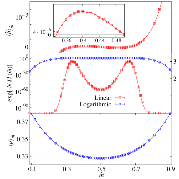
Figure 1: (Color online) Computation of the Helmholtz potential $\Omega_{N}$ and the canonical expectation values from tethered averages in a $D=3$, $L=64$ ferromagnetic Ising model at the critical temperature. The upper panel shows the tethered magnetic field $\langle\hat{b}\rangle_{\hat{m}}$, with an inset zooming in on the region between its two zeros. The statistical errors cannot be seen at this scale (except for the leftmost points in the inset). The integral of this quantity is the Helmholtz potential $\Omega_{N}(\hat{m})$. The middle panel shows the $p(\hat{m})=\exp[-N\Omega_{N}(\hat{m})]$ in a linear (right axis) and in a logarithmic scale (left axis). Finally, the bottom panel shows the tethered expectation values of the energy density $u$. Their integral over the whole $\hat{m}$ range, weighted with $p(\hat{m})$, gives the canonical expectation value $\langle u\rangle=-0.3322894(36)$ (horizontal line). See Ref. martin-mayor:09 for further details on these simulations.

The whole process is illustrated in Figure 1, where we compute the energy density at the critical temperature in an $L=64$ lattice of the $D=3$ Ising model. Notice that the tethered expectation values $\langle u\rangle_{\hat{m}}$ vary in about $10\%$ in our $\hat{m}$ range, but the computation of the effective potential is so precise that the averaged value for the energy, $\langle u\rangle=-0.3322894(36)$, has a relative error of only $\sim 10^{-5}$.

This is the general TMC algorithm for the computation of canonical averages from the Helmholtz potential. As we shall see in some of the applications, sometimes the integration over all phase space in step 4 is not needed and one can use the ensemble equivalence property to recover the $\langle O\rangle$ from the $\langle O\rangle_{\hat{m}}$ through saddle-point equations, remember Eq. (1). In other words, the tethered averages can be physically meaningful by themselves. We note as well that our crystallization study in Sect. 5 is built entirely over the effective-potential, one never uses the $p(\hat{m})$.

As will be shown in the next section, the reconstruction of canonical averages from the combination of tethered averages does not involve any approximation. We can achieve any desired accuracy, provided we use a sufficiently dense grid in $\hat{m}$ (to control systematic errors) and simulate each point for a sufficiently long time (to reduce statistical ones). Table 1 shows the kind of precisions that we can achieve. One could initially think that the computation of the exponential in $p(\hat{m})=\exp[-N\Omega_{N}(\hat{m})]$ would produce unstable or imprecise results for large system sizes. Instead, the combination of self-averaging and no critical slowing down makes the numerical precision grow with $N$.

Table 1: Energy density of the $D=3$ ferromagnetic Ising model computed with the Tethered Monte Carlo method, showing that the reconstruction of canonical averages can be performed with great accuracy. The second column shows the number of points in the $\hat{m}$ grid and the third the number of Monte Carlo sweeps taken on each (we use a cluster update scheme). See martin-mayor:09 for further details on these simulations.

$L$	$N_{\hat{m}}$	MCS	$-\langle u\rangle$
16	91	$10^{6}$	0.344905(35)
32	91	$10^{6}$	0.335730(26)
64	109	$10^{6}$	0.3322894(36)
128	50	$10^{6}$	0.3309831(15)

3 The tethered ensemble

In this section we construct the statistical ensemble that supports the TMC method. We shall consider the case of the $D$-dimensional ferromagnetic Ising model. Reproducing the steps of this derivation for any other system is straightforward. We include details on how to introduce several tethered variables (subsection 3.1). Subsection 3.2 discusses the relationship between tethered and canonical expectation values from the point of view of the ensemble equivalence property.

The Ising model is characterized by the following partition function

$$Z=\sum_{\{s_{\boldsymbol{x}}\}}\exp\biggl{[}\beta\sum_{\langle{\boldsymbol{x}},{\boldsymbol{y}}\rangle}s_{\boldsymbol{x}}s_{\boldsymbol{y}}\biggr{]},$$ (12)

where the angle brackets indicate that the sum is restricted to first neighbors and the spins are $s_{\boldsymbol{x}}=\pm 1$. In this section we will be working at fixed $\beta$. Hence, to lighten the expressions we shall drop the explicit $\beta$ dependencies.

The energy and magnetization of this system are

$$U =Nu=-\sum_{\langle{\boldsymbol{x}},{\boldsymbol{y}}\rangle}s_{\boldsymbol{x}}s_{\boldsymbol{y}}, M =Nm=\sum_{\boldsymbol{x}}s_{\boldsymbol{x}},$$ (13)

($N=L^{D}$ is the number of spins in the system).

The canonical average of a generic observable $O$ is

$$\langle O\rangle=\frac{1}{Z}\sum_{\{s_{\boldsymbol{x}}\}}O(\{s_{i}\})\ \mathrm{e}^{-\beta U}.$$ (14)

Since this is a ferromagnetic system, we may be interested in considering the average value of $O$ conditioned to different magnetization regions. The naive way of doing this would be

$$\langle O|m\rangle=\frac{\bigl{\langle}O\delta\bigl{(}m-\sum_{\boldsymbol{x}}s_{\boldsymbol{x}}/N\bigr{)}\bigr{\rangle}}{\bigl{\langle}\delta\bigl{(}m-\sum_{\boldsymbol{x}}s_{\boldsymbol{x}}/N\bigr{)}\bigr{\rangle}}$$ (15)

The canonical average could then be recovered by a weighted average of the $\langle O|m\rangle$,

$$\langle O\rangle=\sum_{m}\langle O|m\rangle p_{1}(m),\qquad p_{1}(m)={\biggl{\langle}\delta\biggl{(}m-\sum_{\boldsymbol{x}}s_{\boldsymbol{x}}/N\biggr{)}\biggr{\rangle}}$$ (16)

In the thermodynamical limit, the reaction coordinate $m$ varies continuously from $-1$ to $1$. For a finite system, however, there are only $N+1$ possible values of $m$, so $p_{1}(m)$ is a comb-like function.

We want to construct a statistical ensemble where a smooth Helmholtz potential can be defined in finite lattices. In order to do this, the first step is extending the configuration space with a bath $R$ of $N$ Gaussian demons and defining the smooth magnetization $\hat{M}$,

$$\hat{M}=N\hat{m}=M+R.$$ (17)

These demons can be introduced either linearly or quadratically,

$$R^{(\text{Q})} =\sum_{i}\eta_{i}^{2}/2,$$ (18)

$$R^{(\text{L})} =\sum_{i}\eta_{i}.$$ (19)

Now our partition function is

$$Z =\int_{-\infty}^{\infty}\biggl{(}\prod_{i=1}^{N}\frac{\mathrm{d}\eta_{i}}{\sqrt{2\pi}}\biggr{)}\sum_{\{s_{\boldsymbol{x}}\}}\exp\biggl{[}-\beta U-\sum_{i}\eta^{2}_{i}/2\biggr{]},$$ (20)

$$p_{2}(r) =\int_{-\infty}^{\infty}\biggl{(}\prod_{i=1}^{N}\frac{\mathrm{d}\eta_{i}}{\sqrt{2\pi}}\biggr{)}\exp\biggl{[}-\sum_{i}\eta^{2}_{i}/2\biggr{]}\delta(r-R/N)$$ (21)

Notice that the demons are statistically independent from the spins. The convolution of $p_{1}(m)$ and $p_{2}(r)$ then gives the probability density function for $\hat{m}$,

$$p(\hat{m})=\int\mathrm{d}m\mathrm{d}r\ p_{1}(m)p_{2}(r)\delta(\hat{m}-m-r).$$ (22)

So $p(\hat{m})$ is essentially a smooth version of $p_{1}(m)$. We can do an analogous construction for off-lattice systems. In this case, the demons would increase the dispersion in the already continuous $p_{1}(x)$. We can control these fluctuations by considering a tunable number of demons, see (37) and Section 5.

We can now rewrite the canonical average $\langle O\rangle$ as

$$\langle O\rangle=\int\mathrm{d}\hat{m}\ \langle O\rangle_{\hat{m}}\ p(\hat{m}),$$ (23)

where the tethered average $\langle O\rangle_{\hat{m}}$ is

$$\langle O\rangle_{\hat{m}}=\frac{1}{Zp(\hat{m})}\int_{-\infty}^{\infty}\prod_{i=1}^{N}\mathrm{d}\eta_{i}\sum_{s_{\boldsymbol{x}}}O(\{s_{\boldsymbol{x}}\})\ \mathrm{e}^{-\beta U-\sum_{i}\eta^{2}_{i}/2}\delta(\hat{m}-m-R/N).$$ (24)

This way, each $\langle O\rangle_{\hat{m}}$ will have contributions from all the $\langle O|m\rangle$, with a weight that will depend on the distance between $m$ and $\hat{m}$. This generates smooth $\langle O\rangle_{\hat{m}}$ and $p(\hat{m})$, so we can now define the Helmholtz effective potential in our finite lattice as

$$p(\hat{m})=\mathrm{e}^{-N\Omega_{N}(\hat{m})}$$ (25)

It may seem that with our extended configuration space, we have sacrificed too much in order to get smooth functions, but we can actually integrate the demons out with the Dirac deltas:

$$\mathrm{e}^{-N\Omega_{N}(\hat{m})}=\frac{1}{Z}\sum_{\{s_{\boldsymbol{x}}\}}\omega_{N}(\hat{m},\{s_{\boldsymbol{x}}\}),$$ (26)

where the weight $\omega_{N}(\hat{m},\{s_{\boldsymbol{x}}\})$ is, for our linear and quadratic demons (neglecting irrelevant constant factors),

$$\omega^{(\text{Q})}_{N}(\hat{m},\{s_{\boldsymbol{x}}\}) \propto\mathrm{e}^{-\beta U+M-\hat{M}}(\hat{m}-m)^{(N-2)/2}\theta(\hat{m}-m)$$ (27)

$$\omega^{(\text{L})}_{N}(\hat{m},\{s_{\boldsymbol{x}}\}) \propto\mathrm{e}^{-\beta U-(M-\hat{M})^{2}/(2N)}.$$ (28)

In general, $\omega_{N}(\hat{m},\{s_{\boldsymbol{x}}\})$ will be of the following form,

$$\omega_{N}(\hat{m},\{s_{\boldsymbol{x}}\})\propto\mathrm{e}^{-\beta U}\gamma(\hat{m},m),$$ (29)

that is, the thermal component typical of a canonical simulation and a magnetic factor that depends only on $m$ and $\hat{m}$. The weight $\omega_{N}$ defines a new statistical ensemble, so we can now rewrite the tethered averages as

$$\langle O\rangle_{\hat{m}}=\frac{\sum_{\{s_{\boldsymbol{x}}\}}O(\{s_{\boldsymbol{x}}\})\omega_{N}(\hat{m},\{s_{\boldsymbol{x}}\})}{\sum_{\{s_{\boldsymbol{x}}\}}\omega_{N}(\hat{m},\{s_{\boldsymbol{x}}\})}$$ (30)

A particularly important tethered average is the $\hat{m}$-derivative of the effective potential, the tethered magnetic field $\langle\hat{b}\rangle_{\hat{m}}$,

$$\frac{\partial\Omega_{N}}{\partial\hat{m}}=\langle\hat{b}\rangle_{\hat{m}}.$$ (31)

For our two kinds of demons this is

$$\hat{b}^{(\text{Q})} =1-\frac{1/2-1/N}{\hat{m}-m},$$ (32)

$$\hat{b}^{(\text{L})} =\hat{m}-m.$$ (33)

Definition (31), together with the condition that $p(\hat{m})=\mathrm{e}^{-N\Omega_{N}(\hat{m})}$ be normalized, allows us to reconstruct the Helmholtz potential from tethered averages alone. The canonical averages can then be recovered through Eq. (23).

The tethered magnetic field is essentially a measure of the fluctuations in $m$, which illustrates the dual roles the magnetization and magnetic field play in the canonical and tethered formalism. This is further demonstrated by the tethered fluctuation-dissipation formula

$$\frac{\partial\langle O\rangle_{\hat{m}}}{\partial\hat{m}}=\left\langle\frac{\partial O}{\partial\hat{m}}\right\rangle_{\hat{m}}+N[\langle O\hat{b}\rangle_{\hat{m}}-\langle O\rangle_{\hat{m}}\langle\hat{b}\rangle_{\hat{m}}].$$ (34)

Notice that the values of $\hat{m}$ where $\langle\hat{b}\rangle_{\hat{m}}=0$ will define maxima and minima of the effective potential and, hence, of the probability $p(\hat{m})$.

The tethered ensemble is, thus, constructed via a Legendre transformation of the canonical one, that exchanges the roles of the magnetic field and the magnetization. In fact, we can write the canonical partition for a given value of the applied magnetic field in the following way

$$Z(h)=\mathrm{e}^{NF_{N}(h)}=\int\mathrm{d}\hat{m}\ \mathrm{e}^{-N[\Omega_{N}(h)-\beta h\hat{m}]}.$$ (35)

One interesting consequence is that computing canonical averages for non-zero magnetic fields does not imply changing (recomputing) the tethered averages, only their weights,

$$\langle O\rangle(h)=\frac{1}{Z(h)}\int\mathrm{d}\hat{m}\ \langle O\rangle_{\hat{m}}\ \mathrm{e}^{-N[\Omega_{N}(h)-\beta h\hat{m}]},$$ (36)

in other words, we just have to shift the tethered magnetic field, $\langle\hat{b}\rangle_{\hat{m}}\to\langle\hat{b}\rangle_{\hat{m}}-\beta h$.

A final general point concerns the introduction of the Gaussian demons. Our definitions (18) and (19) and subsequent construction make the assumption that there are as many demons as spins. While this choice seems natural, it is by no means a necessity. In fact, in order to control the fluctuations in the reaction coordinate, it may in occasion be interesting to consider a variable number of demons (see Section 5):

$$R_{\alpha} =\frac{1}{\alpha}\sum_{i=1}^{\alpha N}\eta_{i}, \hat{M}=N\hat{m}=M+R_{\alpha},$$ (37)

where $\alpha$ is the tunable parameter. All the computations in this section can be easily reconstructed for this more general case. As an example, the tethered magnetic field with $\alpha N$ linearly added demons is

$$\hat{b}^{(\text{L})}=\alpha(\hat{m}-m).$$ (38)

3.1 Several tethered variables

Throughout this section we have considered an ensemble with only one tethered quantity. However, as we shall see in the following sections, it is often appropriate to consider several reaction coordinates at the same time. The construction of the tethered ensemble in such a study presents no difficulties. We start by coupling reaction coordinates $x_{i}$, $i=1..n$, with $N$ demons each,

$$\hat{X}_{1}=N\hat{x}_{1}=X_{1}+R_{1},\quad\ldots,\quad\hat{X}_{n}=N\hat{x}_{n}=X_{n}+R_{n}.$$ (39)

We then follow the same steps of the previous section, with the consequence that the tethered magnetic field is now a conservative field computed from an $n$-dimensional potential $\Omega_{N}(\hat{{\boldsymbol{x}}})$

$$\boldsymbol{\nabla}\Omega_{N} =\bigl{(}\partial_{\hat{x}_{1}}\Omega_{N},\ldots,\partial_{\hat{x}_{n}}\Omega_{N}\bigr{)}=\hat{\boldsymbol{B}}$$ (40)

$$\hat{\boldsymbol{B}} =(\langle\hat{b}_{1}\rangle_{\hat{\boldsymbol{x}}},\ldots,\langle\hat{b}_{n}\rangle_{\hat{\boldsymbol{x}}}),$$ (41)

and each of the $\hat{b}_{i}$ is of the same form as in the case with only one tethered variable. Similarly, the tethered weight of Eq. (29) is now

$$\omega^{(n)}(\hat{\boldsymbol{x}},\{s_{\boldsymbol{x}}\})=\mathrm{e}^{-\beta U}\gamma(\hat{x}_{1},x_{1})\gamma(\hat{x}_{2},x_{2})\cdots\gamma(\hat{x}_{n},x_{n}).$$ (42)

3.2 Ensemble equivalence and spontaneous symmetry breaking

Throughout this section we have implicitly assumed that the final goal of a Tethered Monte Carlo computation is eventually to reconstruct the canonical averages. As we shall see in some of the applications, however, this is not always the case. One example is the computation of the hyperscaling violations exponent of the RFIM in fernandez:11b , which is made directly from $\Omega_{N}$.

Still, most of the time the averages in the canonical ensemble are the ones with a more direct physical interpretation (fixed temperature, fixed applied field, etc.). In principle, their computation implies reconstructing the whole effective potential $\Omega_{N}$ and using it to integrate over the whole coordinate space, as in (23) or, more generally, (36). Sometimes, however, the connection between the tethered and canonical ensembles is easier to make. Let us return to our ferromagnetic example, with a single tethered quantity $m$. Recalling the expression of the canonical partition function in terms of $\Omega_{N}$ for finite $h$, Eq. (35), a steepest-descent tells us that, for large $N$, the integral is dominated by one saddle point such that

$$\partial_{\hat{m}}[\Omega_{N}(\hat{m})-\beta h\hat{m}]=0\qquad\Longrightarrow\qquad\langle\hat{b}\rangle_{\hat{m}}=\beta h.$$ (43)

Clearly, this saddle point (actually, the global minimum of the effective potential) rapidly grows in importance with the system size $N$, to the point that we can write

$$\lim_{N\to\infty}\langle O\rangle(h)=\lim_{N\to\infty}\langle O\rangle_{\hat{m}(h)}.$$ (44)

That is, in the thermodynamical limit we can identify the canonical average for a given applied magnetic field $h$ with the tethered average computed at the saddle point defined by $h$ (which is nothing more than the point where the tethered magnetic field coincides with the applied magnetic field).

This ensemble equivalence property would be little more than a curiosity if it were not for the fact that the convergence is actually extremely fast (see fernandez:09 for a study). Therefore, in many practical applications the equivalence (44) can be made even for finite lattices (see Section 4 below for an example).

The saddle-point approach can be applied to systems with spontaneous symmetry breaking. In the typical analysis, one has to perform first a large-$N$ limit and then a small-field one (this is troublesome for numerical work, where one usually has to consider non-analytical observables such as $|m|$). In the tethered ensemble we can implement this double limit in an elegant way by considering a restricted range in the reaction coordinate from the outset (see fernandez:09 for a straightforward example in the Ising model and Section 4.4 for a more subtle one).

4 The diluted antiferromagnet in a magnetic field

In this section we consider the application of the tethered formalism to the diluted antiferromagnet in an external field (DAFF), one of the simplest physical systems showing cooperative behavior in the presence of quenched disorder. A good experimental introduction to this system can be found in belanger:97 . It was shown in fishman:79 ; cardy:84 that the DAFF belongs to the same universality class as the random field Ising model (RFIM), a system more amenable to analytical treatment (see nattermann:97 for a review and dedominicis:06 for a field-theoretical approach).

Experimental, Monte Carlo and analytical studies of the DAFF/RFIM agree that this system experiences a phase transition for more than two spatial dimensions. At low temperatures, if the applied magnetic field $h$ is small, the DAFF remains in an antiferromagnetically ordered state. If the magnetic field (or the temperature) is raised, however, the ferromagnetic part of the Hamiltonian weakens the antiferromagnetic correlations and the DAFF crosses into a paramagnetic state. This transition occurs across a smooth critical surface in the $(\beta,h,p)$ space ($p$ characterizes the dilution of the system).

That much is generally accepted. However, despite decades of interest on this system, most of the details of this phase transition remain controversial. For instance, the analytical work on the RFIM favors a second-order scenario. Most recent numerical and experimental studies of the DAFF agree vink:10 ; hartmann:01 ; slanic:99 ; ye:02 , but some recent work sourlas:99 ; maiorano:07 has found signatures characteristic of first-order transitions (such as metastability, or a very low critical exponent $\beta$ that raises the possibility of a discontinuous transition). These apparent inconsistencies between numerical work and analytical predictions have even led some researchers to consider the possibility that the RFIM and DAFF may not be equivalent after all. Even allowing for this possibility, the comparison of numerical and experimental work on the DAFF has not always yielded completely satisfactory results. For instance, some experiments have reported a divergent specific heat belanger:83 ; belanger:98 , not observed numerically hartmann:01 .

The problems on the numerical front can be understood if we notice that the DAFF is particularly ill-suited to numerical investigation in the canonical ensemble. On the one hand, the system suffers from a very severe thermally activated critical slowing down, where the characteristic times grow as $\log\tau\sim\xi^{\theta}$, with $\theta\approx 1.5$. On the other hand, the statistical averages in the canonical ensemble are dominated by extremely rare events, which gives rise to strong violations of self-averaging parisi:02 .

Finally, some crucial physical results are hardly accessible to a canonical computation. Perhaps the most important is the hyperscaling violations exponent $\theta$. This is an additional critical exponent that one must introduce to make the theory consistent, and that modifies the standard hyperscaling relation, $2-\alpha=D\nu$, in the following way,

$$2-\alpha=\nu(D-\theta).$$ (45)

In the canonical ensemble, the exponent $\theta$ is associated to the free-energy barrier between the ordered and the disordered phase vink:10 ; fischer:11 , $\Delta F\propto L^{\theta}$. Hence, it is a good marker to distinguish a first-order scenario ($\theta\geq D-1$) from a second-order one ($\theta<D-1$). At the same time, it is extremely difficult to compute with standard Monte Carlo methods.

In fernandez:11b we performed a Tethered Monte Carlo study of this system and found that many of the problems with previous numerical work were solved. As one wishes to ascertain that a first-order transition with the magnetic field is not present, it is only natural to tether the conjugate magnitude, the standard magnetization. On the other hand, the largest barriers are associated to the order parameter (the staggered magnetization, see below), which was also tethered.

A consistent picture of the phase transition, which was shown to be continuous, emerged. Self-averaging was restored and thermalization greatly accelerated. We were able to obtain the three independent critical exponents and found a (slow) divergence of the specific heat, in accordance with experiments. In particular, the critical exponent $\theta$, so elusive to canonical computations, was determined with some precision: $\theta=1.47(2)$ (the free-energy barriers related to $\theta$ are immediately translated into effective-potential barriers, readily computed with the methods of the previous sections).

In the remainder of this section we shall explain in some detail the application of the tethered formalism to this problem. We first define the model and some basic observables in 4.1. This is followed in 4.2 by an examination of the DAFF with traditional (canonical) methods, that expands on the problems discussed above. Next, we construct a tethered formalism adapted to the DAFF and discuss how to restore self-averaging to the disorder averages. In 4.5 we report the parameters of our simulations and in 4.6 we discuss their thermalization and possible optimizations. Finally, in 4.7 we include a geometrical investigation of the instanton configurations, not included in fernandez:11b . This serves as a good example of how a tethered computation is not restricted to reproducing canonical results more efficiently, but can access interesting information that is completely hidden from a canonical study.

4.1 Model and observables

We consider the diluted antiferromagnet in a field (DAFF) on a square lattice with $N=L^{3}$ nodes and periodic boundary conditions

$$\mathcal{H}=\sum_{\langle\boldsymbol{x},\boldsymbol{y}\rangle}\epsilon_{\boldsymbol{x}}s_{\boldsymbol{x}}\epsilon_{\boldsymbol{y}}s_{\boldsymbol{y}}-h\sum_{\boldsymbol{x}}\epsilon_{\boldsymbol{x}}s_{\boldsymbol{x}}.$$ (46)

In addition to the Ising spins ($s_{\boldsymbol{x}}=\pm 1$), the Hamiltonian includes occupation variables $\epsilon_{\boldsymbol{x}}$. These are randomly distributed according to $P(\epsilon)=p\delta(\epsilon-1)+(1-p)\delta(\epsilon)$. Throughout this paper we shall consider a spin concentration of $p=0.7$. This value is very far from the percolation threshold of $p\approx 0.31$ stauffer:84 , but not so high as to be dominated by the pure case ($p=1$). The $\epsilon_{\boldsymbol{x}}$ are quenched variables, which means that we should perform first the thermal average for each choice of the $\{\epsilon_{\boldsymbol{x}}\}$ and only afterwards compute the disorder average. In the canonical ensemble, we shall denote the thermal average by $\langle\cdots\rangle$ and the disorder average by $\overline{(\cdots)}$.

For each spin configuration, we can define the standard and staggered magnetizations

$$M = Nm=\sum_{\boldsymbol{x}}\epsilon_{\boldsymbol{x}}s_{\boldsymbol{x}},$$ (47)

$$M_{\mathrm{s}} = Nm_{\mathrm{s}}=\sum_{\boldsymbol{x}}\epsilon_{\boldsymbol{x}}s_{\boldsymbol{x}}\pi_{\boldsymbol{x}},\quad\pi_{\boldsymbol{x}}=\mathrm{e}^{\mathrm{i}\pi\sum_{\mu=1}^{D}x_{\mu}}.$$ (48)

We shall distinguish between the energy $E$ and the first-neighbors connectivity $U$,

$$E = Ne=\sum_{\langle\boldsymbol{x},\boldsymbol{y}\rangle}\epsilon_{\boldsymbol{x}}s_{\boldsymbol{x}}\epsilon_{\boldsymbol{y}}s_{\boldsymbol{y}}-h\sum_{\boldsymbol{x}}\epsilon_{\boldsymbol{x}}s_{\boldsymbol{x}},$$ (49)

$$U = Nu=\sum_{\langle\boldsymbol{x},\boldsymbol{y}\rangle}\epsilon_{\boldsymbol{x}}s_{\boldsymbol{x}}\epsilon_{\boldsymbol{y}}s_{\boldsymbol{y}}.$$ (50)

4.2 The DAFF in canonical Monte Carlo simulations

In this section we shall explain the limitations inherent in a canonical study and demonstrate how the tethered formalism can be used to gain more information about the system. In order to do so, we shall first carry out a comparative study of a single disorder realization (sample) in both the canonical and tethered ensembles. We shall then explain how to perform the disorder average in the tethered formalism and provide the motivation for the approach taken in this study.

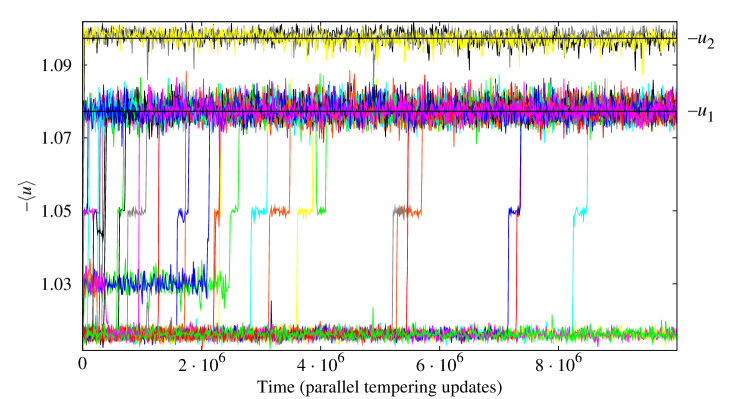
Figure 2: (Color online) Monte Carlo histories of the first-neighbor connectivity density $u$ for different runs of the same sample in a canonical parallel tempering simulation ($L=24$, $T=1.6,h=2.4,p=0.7$). After a variable simulation time, the runs eventually reach one of two local minima (labeled by $u_{1}$ and $u_{2}$), but the simulations are not long enough for us to see any tunneling between the two.

We have performed several parallel-tempering hukushima:96 ; marinari:98b simulations of the same disorder realization for an $L=24$ system. In Figure 2 we can see how after some time the systems reach one of two local minima of the effective potential, with first-neighbor connectivities, Eq. (50) $u^{(1)}=-1.07735(8)$ and $u^{(2)}=-1.0973(7)$. The corresponding energy densities, Eq. (49), are $e^{(1)}=-1.37608(2)$ and $e^{(2)}=-1.3820(2)$.

On the basis of these data, one would think that these two minima are relevant to the equilibrium of this particular sample, so that if we wait a sufficiently long time we will eventually see the system tunnel back and forth between the two of them. This apparent metastability could lead to the interpretation that the system is experiencing a first-order phase transition. There are two problems, however. The first one is that we have not actually seen the tunneling in any of our simulations. In other words, canonical parallel-tempering is not able to thermalize the system in a reasonable amount of time. Notice that obtaining the two minima in separate simulations is not enough, we need to see the tunneling in order to know their relative weight.

The second problem is illustrated on Figure 3. In it we represent a scatter plot of the staggered magnetization against $u$ for the runs in Figure 2. It is readily apparent that the two local minima correspond to antiferromagnetic systems with opposite sign of the order parameter ($m_{\text{s}}^{(1)}=0.5023(3)$, $m_{\text{s}}^{(2)}=-0.543(3))$, so the observed metastability does not correspond to the disordered-antiferromagnetic transition in which we are interested. A canonical simulation cannot separate the different staggered magnetization sectors, so a study in this statistical ensemble will always be contaminated by this spurious metastability and dominated by extremely rare events.

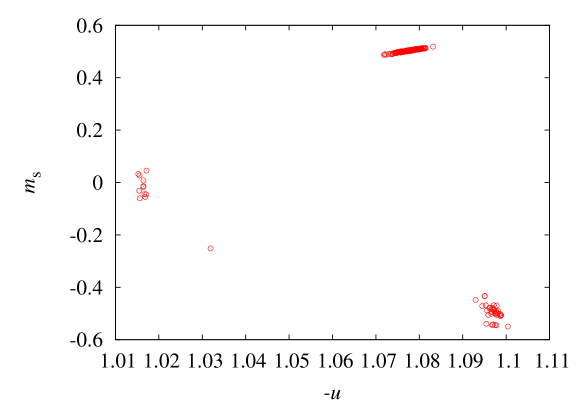
Figure 3: (Color online) Scatter plot of the first-neighbor connectivity and the staggered magnetization, as computed on the very last $0.1\%$ of the Monte Carlo history for the simulations in Figure 2. Most of the simulations have reached one of two local minima with opposite staggered magnetization.

4.3 The DAFF in the tethered ensemble

Following the results of our canonical investigation, the obvious quantity to tether in the DAFF is the staggered magnetization $m_{\text{s}}$. This would, for instance, allow us to study separately the different saddle points, as discussed in Section 3.2, and, through the Helmholtz potential, to determine their relative weight, without any need for exponentially slow tunneling. In addition, since we are interested in a transition at non-zero magnetic field $h$, in which metastability could also appear, we will tether the standard magnetization $m$.

We, therefore, have a two-component tethered magnetic field

$$\boldsymbol{\nabla}\Omega_{N}(\hat{m},\hat{m}_{\text{s}})=\biggl{(}\frac{\partial\Omega_{N}(\hat{m},\hat{m}_{\text{s}})}{\partial\hat{m}},\ \frac{\partial\Omega_{N}(\hat{m},\hat{m}_{\text{s}})}{\partial\hat{m}_{\text{s}}}\biggr{)}=\bigl{(}\langle\hat{b}\rangle_{\hat{m},\hat{m}_{\text{s}}},\langle\hat{b}_{s}\rangle_{\hat{m},\hat{m}_{\text{s}}}\bigr{)}$$ (51)

We use quadratically added demons, as in Eq. (18). Therefore,

$$\hat{b} =1-\frac{1/2-1/N}{\hat{m}-m},$$ (52)

$$\hat{b}_{\text{s}} =1-\frac{1/2-1/N}{\hat{m}_{\text{s}}-m_{\text{s}}}.$$ (53)

In general, canonical averages in the presence of an external magnetic field with a regular component $h$ and a staggered component $h_{\text{s}}$ can be recovered through the Legendre transform equation:

$$\langle O\rangle(h,h_{\text{s}})=\frac{\int\mathrm{d}\hat{m}\int\mathrm{d}\hat{m}_{\text{s}}\ \langle O\rangle_{\hat{m},\hat{m}_{\text{s}}}\ \mathrm{e}^{-N[\Omega_{N}(\hat{m},\hat{m}_{\text{s}})-\hat{m}\beta h-\hat{m}_{\text{s}}\beta h_{\text{s}}]}}{\int\mathrm{d}\hat{m}\int\mathrm{d}\hat{m}_{\text{s}}\ \mathrm{e}^{-N[\Omega_{N}(\hat{m},\hat{m}_{\text{s}})-\hat{m}\beta h-\hat{m}_{\text{s}}\beta h_{\text{s}}]}},$$ (54)

although here we shall be interested in $h_{\text{s}}=0$, so we shall use the notation

$$\langle O\rangle(h)=\langle O\rangle(h,h_{\text{s}}=0).$$ (55)

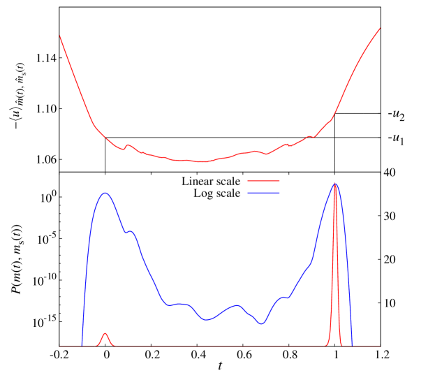
Figure 4: (Color online) Top: Result of a tethered simulation for the sample of Figure 2. The two saddle points are joined by a straight path $(\hat{m}(t),\hat{m}_{\text{s}}(t))$, along which we measure the energy density $\langle u\rangle_{\hat{m}(t),\hat{m}_{\text{s}}(t)}$. For $t=0$ and $t=1$ we reproduce the energies of the local minima obtained in the canonical simulation. Bottom: Relative weight of the points along the simulated path, obtained from the line integral of the tethered magnetic field (52) (see text).

The computation of these canonical averages following the procedure described in Section 2 is very complicated. It would involve the non-trivial computation of a two-dimensional potential from its gradient, after running a set of many simulations in a two-dimensional grid in $(\hat{m},\hat{m}_{\text{s}})$. As we shall see in the following, the practical application is simpler than that. This is because for a given value of $h$ only a very small region of the configuration space $(\hat{m},\hat{m}_{\text{s}})$ will have a relevant weight in (54), as discussed in Section 3.2. Therefore, due to the ensemble equivalence property, we will be able to relate canonical and tethered averages through saddle-point equations

$$\begin{cases}\displaystyle\frac{\partial\Omega_{N}}{\partial\hat{m}}&=\langle\hat{b}\rangle_{\hat{m},\hat{m}_{\mathrm{s}}}=\beta h,\\ \\ \displaystyle\frac{\partial\Omega_{N}}{\partial\hat{m}_{\mathrm{s}}}&=\langle\hat{b}_{\mathrm{s}}\rangle_{\hat{m},\hat{m}_{\mathrm{s}}}=0.\end{cases}$$ (56)

As an example we can return to the sample of Section 4.2. Using a canonical parallel-tempering simulation, we had identified two local minima, but were unable to determine their relative weights. We can perform now this study in the tethered formalism.

The first step in this computation is identifying the values of $(\hat{m},\hat{m}_{\text{s}})$ that correspond to the local minima using (56). Notice that from the canonical simulation we know the values of $m^{(i)}$ and $m_{\text{s}}^{(i)}$, so, using Eq. (52), $\hat{m}_{\text{s}}^{(i)}\simeq m_{\text{s}}^{(i)}+1/2$ and $\hat{m}^{(i)}\simeq m^{(i)}+1/(2(1-\beta h))$. From these starting guesses the actual minima are readily found. The strategy is then clear: by performing the line integral of

$$\hat{\boldsymbol{B}}=\bigl{(}\langle\hat{b}\rangle_{\hat{m},\hat{m}_{\text{s}}}-\beta h,\ \ \langle\hat{b}_{\mathrm{s}}\rangle_{\hat{m},\hat{m}_{\text{s}}}\bigr{)}$$ (57)

along a path connecting the two saddle points we immediately obtain their potential difference or, equivalently, the ratio between their weights. The very same procedure, carried out for hard-spheres, is depicted in Fig. 15.

Figure 4 shows the result of this computation. For our connecting path we use the straight line $(\hat{m}(t),\hat{m}_{\text{s}}(t))=(\hat{m}^{(1)},\hat{m}_{\text{s}}^{(1)})(1-t)+(\hat{m}^{(2)},\hat{m}_{\text{s}}^{(2)})$. As we can see in the upper panel, the tethered averages $\langle u\rangle_{\hat{m}(t),\hat{m}_{\text{s}}(t)}$ for $t=0$ and $t=1$ closely match $u^{(1)}$ and $u^{(2)}$, confirming ensemble equivalence. The lower panel shows the relative weight $P(\hat{m}(t),\hat{m}_{\text{s}}(t))$ of the points along the path. In accordance with (54) this is simply

$$P(\hat{m}(t),\hat{m}_{\text{s}}(t))=\mathrm{e}^{-N\bigl{[}\Omega_{N}(\hat{m}(t),\hat{m}_{\text{s}}(t))-\beta h\hat{m}(t)\bigr{]}},$$ (58)

where we have chosen the zero in $\Omega_{N}$ so that the weight of the whole path is normalized.

One of the two peaks is seen to have about ten times more importance than the other. Interestingly, we see that they are separated by a region of very low probability, which explains the difficulty of the canonical simulations to tunnel between the two of them. The large number of intermediate maxima and minima in the effective potential are a real effect, and not fluctuations, as we shall see more clearly in the next section.

4.4 Self-averaging and the disorder average

In order to perform a quantitative analysis of the DAFF, we have to simulate a large number of samples and perform the disorder average. The naive way of doing this for a system with quenched disorder would be to measure $\hat{\boldsymbol{B}}$ and construct $\Omega_{N}$ for each sample, then use Eq. (54) to compute all the physically relevant $\langle O\rangle(h)$. Only then would we average $\langle O\rangle(h)$ over the disorder.

This approach is, however, paved with pitfalls. First of all, computing a two-variable $\Omega_{N}(\hat{m},\hat{m}_{\text{s}})$ from a two-dimensional $(\hat{m},\hat{m}_{\text{s}})$ grid is not an easy matter. In the previous section we avoided this problem by finding the local minima first and then evaluating $\Omega_{N}$ only along a path joining them. But this cannot be done efficiently and safely for a large number of samples. Even if it could be done, the free-energy landscape of each sample is very complicated, with many local minima, several of which could be relevant to the problem, so a very high resolution would be needed on the simulation grid.

Finally, even reliably and efficiently computing the canonical averages $\langle O\rangle(h)$ would not be the end of our problems. Indeed, it is a well known fact that random systems often suffer from violations of self-averaging aharony:96 ; wiseman:98 ; malakis:06 . This phenomenon has recently been studied in detail for the RFIM parisi:02 , where the violations of self-averaging are shown to be especially severe. In this section we address all these problems and demonstrate the computational strategy followed in our study of the DAFF.

The first step is ascertaining whether the tethered averages themselves are self-averaging or not. We already know that, since we are going to be working with a large regular external field $h$, the relevant region for the regular magnetization $m$ (and hence $\hat{m}$) is going to be very narrow. Therefore, we are going to explore the whole range of $\hat{m}_{\text{s}}$ for a fixed value of $\hat{m}=0.12$.

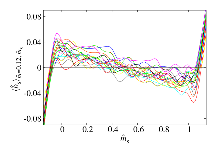
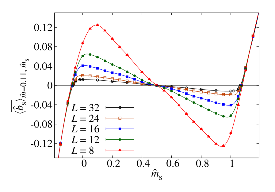
Figure 5: (Color online) Left: Staggered component of the tethered magnetic field, $\langle\hat{b}\rangle_{\hat{m},\hat{m}_{\text{s}}}$ for $\hat{m}=0.12$ as a function of $\hat{m}_{\text{s}}$. We plot the results for several samples of an $L=24$ system at $\beta=0.625$. The curves are cubic splines interpolated from $33$ simulated points. Right: Disorder-averaged $\overline{\langle\hat{b}_{\text{s}}\rangle}_{\hat{m},\hat{m}_{\text{s}}}$ for the same smooth magnetization and temperature as the left panel, for all our system sizes. The plot shows the different behavior of the regions inside the gap, where the staggered magnetic field goes to zero as $L$ increases, and outside of it, where there is a non-zero enveloping curve.

We have plotted the staggered tethered magnetic field $\langle\hat{b}_{\text{s}}\rangle_{\hat{m}=0.12,\hat{m}_{\text{s}}}$ for $20$ samples of an $L=24$ system at $\beta=0.625$ in Figure 5—left. The different curves have a variable number of zeros, but all of them have at least three: one in the central region and two roughly symmetrical ones for large staggered magnetization. The positions of the two outermost zeros clearly separate two differently behaved regions. Inside of the gap the sample-to-sample fluctuations are chaotic, while outside of it the sheaf of curves even seems to have an envelope. This impression is confirmed in the right panel of Figure 5, where we show the sample-averaged tethered magnetic field for several system sizes.

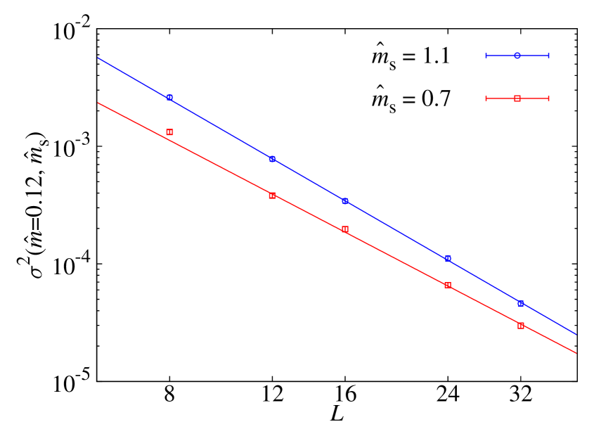
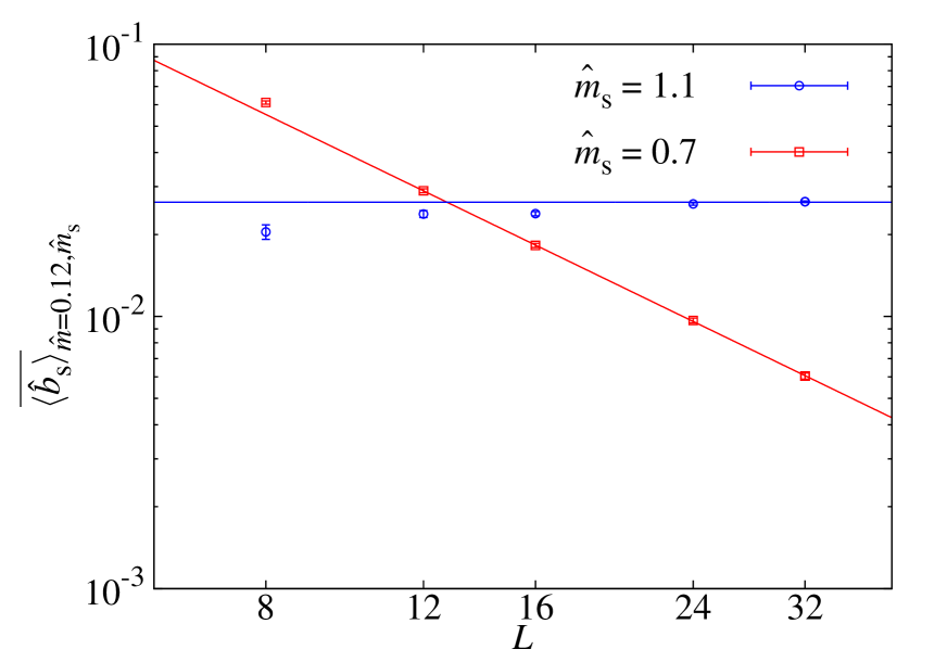
Figure 6: (Color online) Left: Sample-to-sample fluctuations in the staggered component of the tethered magnetic field, Eq. (59), against system size. We show two sets of points, both at $\beta=0.625$ and $\hat{m}=0.12$, but at different values of $\hat{m}_{\text{s}}$. The red curve, corresponding to $\hat{m}_{\text{s}}=0.7$ is right inside the gap defined by the outermost zeros in Figure 5, while the blue curve ($\hat{m}_{\text{s}}=1.1$) is outside. Both are shown to decay with a power law. Right: Disorder average $\overline{\langle\hat{b}_{\text{s}}\rangle}_{\hat{m},\hat{m}_{\text{s}}}$ for the systems of the left panel. Inside the gap, the field goes to zero with $L$; outside it has a finite limit.

In order to quantify this observation we can study the fluctuations of the disorder-averaged $\overline{\langle\hat{b}_{\text{s}}\rangle}_{\hat{m},\hat{m}_{\text{s}}}$,

$$\sigma^{2}(\hat{m},\hat{m}_{\mathrm{s}}) = \overline{\left({\langle\hat{b}_{\mathrm{s}}\rangle}_{\hat{m},\hat{m}_{\mathrm{s}}}-\overline{\langle\hat{b}_{\mathrm{s}}\rangle}_{\hat{m},\hat{m}_{\mathrm{s}}}\right)^{2}}\ .$$ (59)

This quantity is plotted on the left panel of Figure 6. As we can see, it goes to zero as a power in $L$, so we also plot fits to

$$\sigma^{2}(\hat{m}=0.12,\hat{m}_{\text{s}})=A(\hat{m}_{\text{s}})L^{c(\hat{m}_{\text{s}})}.$$ (60)

This would seem like a very good sign, because it could be indicative of self-averaging behavior. However, it is not the whole story. If we recall the right panel of Figure 5, we see that inside the gap the tethered magnetic field itself, not only its fluctuations, goes to zero as $L$ increases. In fact, as shown in Figure 6, for $\hat{m}_{\text{s}}=0.7$, $\sigma^{2}\sim L^{-2.5}$, while $\overline{\langle\hat{b}_{\text{s}}\rangle}_{\hat{m},\hat{m}_{\text{s}}}\sim L^{-1.6}$. This means that the relative fluctuations $\sigma/\overline{\langle\hat{b}_{\text{s}}\rangle}_{\hat{m},\hat{m}_{\text{s}}}$ do not decrease with increasing $L$. For the point outside the gap, however, the disorder average of the tethered magnetic field reaches a plateau. Furthermore, the fluctuations decay with $c=2.94(7)$, which is compatible with the value $c=D$ that one would expect in a self-averaging system.

In physical terms, this analysis means that the local minima for a small, but non-zero, value of the applied staggered magnetic field $h_{\text{s}}$ would be self-averaging. We can now recall the well-known recipe for dealing with spontaneous symmetry breaking: consider a small applied field and take the thermodynamical limit before making the field go to zero. Translated to the DAFF, this means that we should solve the saddle-point equations (56) on average, rather than sample by sample, and then take the $h_{\text{s}}\to 0$ limit on the results,

$$\begin{cases}\displaystyle\frac{\partial\overline{\Omega}_{N}}{\partial\hat{m}}&=\overline{\langle\hat{b}\rangle}_{\hat{m},\hat{m}_{\mathrm{s}}}=\beta h,\\ \\ \displaystyle\frac{\partial\overline{\Omega}_{N}}{\partial\hat{m}_{\mathrm{s}}}&=\overline{\langle\hat{b}_{\mathrm{s}}\rangle}_{\hat{m},\hat{m}_{\mathrm{s}}}=0^{+}.\end{cases}$$ (61)

In other words, we are considering the disorder average of a thermodynamical potential, $\Omega_{N}$, different from the free energy. This approach was first introduced in fernandez:08 , in a microcanonical context (the averaged potential was in that case the entropy).

Notice that for the regular component of the tethered magnetic field we are always going to work with a finite value of the external field $h$. Therefore, the integral in (54) is going to be completely dominated by an extremely narrow $\hat{m}$ range. Therefore, we can consider different values of $\hat{m}$ separately and relate them to the particular $h$ that generates a local minimum at that magnetization. This is best accomplished by integrating the disorder-averaged tethered magnetic field along the path $\bigl{(}\hat{m}=\hat{m}_{0},\hat{m}_{\text{s}}(t)\bigr{)}$. In this way we obtain the probability distribution of $\hat{m}_{\text{s}}$, conditioned to $\hat{m}=\hat{m}_{0}$, which we will denote by $p(\hat{m}_{\text{s}}|\hat{m}_{0})$ (Figure 7). This probability density function can be used to average over $\hat{m}_{\text{s}}$ for fixed $\hat{m}$,

$$\overline{\langle O\rangle}_{\hat{m}}=\int\mathrm{d}\hat{m}_{\text{s}}\ p(\hat{m}_{\text{s}}|\hat{m})\overline{\langle O\rangle}_{\hat{m},\hat{m}_{\text{s}}}=\int\mathrm{d}\hat{m}_{\text{s}}\ \overline{\langle O\rangle}_{\hat{m},\hat{m}_{\text{s}}}\mathrm{e}^{-N\overline{\Omega}_{N}(\hat{m}_{\text{s}}|\hat{m})},$$ (62)

where

$$\frac{\partial\overline{\Omega}_{N}(\hat{m}_{\text{s}}|\hat{m})}{\partial\hat{m}_{\text{s}}}=\overline{\langle\hat{b}_{s}\rangle}_{\hat{m},\hat{m}_{\text{s}}}\ .$$ (63)

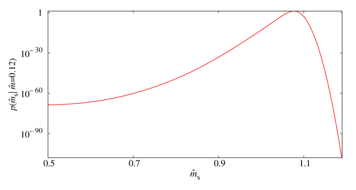
Figure 7: (Color online) Disorder-averaged probability density function of $\hat{m}_{\text{s}}$ conditioned to $\hat{m}=0.12$ for the system of Figure 5.

With this process we have integrated out the dependence on $\hat{m}_{\text{s}}$. We now have a series of smooth functions $\overline{\langle O\rangle}_{\hat{m}}$, together with a smooth one-to-one function $h(\hat{m})=\overline{\langle\hat{b}\rangle}_{\hat{m}}/\beta$. Remembering our discussion of ensemble equivalence in Section 3.2, we shall make the approximation

$$\overline{\langle O\rangle}(h)\simeq\overline{\langle O\rangle}_{\hat{m}(h)}.$$ (64)

At any rate, we remark that the r.h.s. is better suited for reproducing the physics of experimental samples.

Finally, let us mention that some of the physical observables are correlated with the distribution of the $\epsilon_{\boldsymbol{x}}$. This can be exploited to reduce the statistical errors of their sample averages, using the technique of control variates fernandez:09c ; yllanes:11 .

4.5 Our simulations

Table 2: Parameters of our simulations. For each of the $N_{\mathrm{samples}}$ disorder realizations for each $L$, we run $N_{\hat{m}}\times N_{\hat{m}_{\mathrm{s}}}$ tethered simulations with temperature parallel tempering. The $N_{T}$ participating temperatures are evenly spaced in the interval $[1.6,2.575]$. For each size we report the minimum number of Monte Carlo steps (Metropolis sweep + parallel tempering). After the application of our thermalization criteria, some of the simulations for $L\geq 24$ needed to be extended, leading to a higher average number of Monte Carlo steps ($N_{\mathrm{MC}}^{\mathrm{av}}$).

$L$	$N_{\mathrm{samples}}$	$N_{T}$	$N_{\hat{m}}$	$N_{\hat{m}_{\mathrm{s}}}$	$N_{\mathrm{MC}}^{\mathrm{min}}$	$N_{\mathrm{MC}}^{\mathrm{av}}$
8	1000	20	5	31	$7.7\times 10^{5}$	$7.7\times 10^{5}$
12	1000	20	5	35	$7.7\times 10^{5}$	$7.7\times 10^{5}$
16	1000	20	5	35	$7.7\times 10^{5}$	$7.7\times 10^{5}$
24	1000	40	5	33	$7.7\times 10^{5}$	$9.3\times 10^{5}$
32	700	40	4	25	$1.5\times 10^{6}$	$5.5\times 10^{6}$

We can infer several useful conclusions from the analysis of the previous section

• The disorder average should be performed on the tethered observables, before computing the effective potential.

• It is best to analyze several values of $\hat{m}$ separately, since the average over $\hat{m}_{\text{s}}$ for each fixed $\hat{m}$ can be unambiguously related to the canonical average via $h(\hat{m})=\overline{\langle\hat{b}\rangle}_{\hat{m}}/\beta$. In this way, we can study the phase transition that arises by varying the applied magnetic field at fixed $\beta$.

• For fixed $\hat{m}$ the conditioned probability $p(\hat{m}_{\text{s}}|\hat{m})$ has two narrow, symmetric peaks, separated by a region with extremely low probability.

Therefore, we have carried out the following steps

1. Select an appropriate grid of $\hat{m}$ values. This should be wide enough to include the critical point for the simulation temperature, and fine enough to detect the fluctuations of $\overline{\langle O\rangle}_{\hat{m}}$. These turn out to be very smooth functions of $\hat{m}$, so a few values of this parameter suffice fernandez:11b .

2. For each value of $\hat{m}$, select an appropriate grid of $\hat{m}_{\text{s}}$. We start with evenly spaced points and after a first analysis add more values of $\hat{m}_{\text{s}}$ in the neighborhood of the minima, as this is the more delicate and relevant region.

3. The simulations for each $(\hat{m},\hat{m}_{\text{s}})$ are carried out with the Metropolis update scheme of section 2.1. In addition, we use parallel tempering (attempting to exchange configurations at neighboring temperatures). This is not needed in order to thermalize the system for $L<32$, but it is convenient since we also study the temperature dependence of some observables. Furthermore, the use of parallel-tempering provides a reliable thermalization check (see the Appendix, particularly section A.1).

From Figure 7 it seems that, in addition, it would pay to restrict the simulations to a narrow range of $\hat{m}_{\text{s}}$ around the peaks, since the tethered values for $\hat{m}_{\text{s}}$ away from them cannot possibly contribute to the average. This is true but for one exception, the computation of the hyperscaling violation exponent $\theta$, which requires that the whole range be explored (see fernandez:11b ).

The parameters of our simulations are presented on Table 2. The table lists the number $N_{\hat{m}}$ of values in our $\hat{m}$ grid and the number of points in the $\hat{m}_{\mathrm{s}}$ grid for each, so the total number of tethered simulations for each sample is $N_{\hat{m}}\times N_{\hat{m}_{\mathrm{s}}}$.

The number of Monte Carlo steps in each tethered simulation is adapted to the autocorrelation time (see next section), the table lists the minimum length $N_{\text{MC}}^{\text{min}}$ and the average length $N_{\text{MC}}^{\text{av}}$ for each lattice size.

4.6 Thermalization and metastability in the tethered simulations

We have assessed the thermalization of our simulations through the autocorrelation times of the system, computed from the analysis of the parallel tempering dynamics (see Section A.1). We require a simulation time longer than $100\tau_{\mathrm{int}}$. As a fail-safe mechanism, we compute the time $t_{\mathrm{hot}}$ that each configuration spends in the upper half of the temperature range. If any of these is less than a third of the median $t_{\mathrm{hot}}$, we double the simulation time, considering that the simulation is too short to allow a good determination of $\tau_{\mathrm{int}}$. This process is only followed for $L\geq 24$. For smaller sizes we have simply made the minimum simulation time large enough to thermalize all samples.

The distribution of correlation times for our different samples turns out to be dependent on the value of $(\hat{m},\hat{m}_{\mathrm{s}})$. Considering first the variation of the average $\tau_{\mathrm{int}}$ with $\hat{m}_{\mathrm{s}}$ at fixed $\hat{m}$, we see that the minimum and its adjoining region are much easier to thermalize (Figure 8). This region coincides with the only points that have a non-negligible probability density (Figure 7), i.e., the only points that contribute to the computation of the $\overline{\langle O\rangle}_{\hat{m}}$. This fact suggests a possible optimization, that we will discuss in Section 4.6.1.

A second interesting result comes from studying the evolution of the $\tau_{\mathrm{i}nt}$ with $\hat{m}$. Figure 9 represents the histogram of autocorrelation times for $\hat{m}_{\mathrm{s}}=0.8$ (in the ‘hard’ region) for two values of $\hat{m}$. The distribution for $\hat{m}=0.12$ has a much heavier tail. It is shown in fernandez:11b that this is due to the onset of a phase transition.

The difficulty in thermalizing some samples stems from the coexistence of several metastable states, even for fixed $(\hat{m},\hat{m}_{\mathrm{s}})$. In Figure 10 we represent the time evolution of the energy $u$ for several temperatures of the same sample ($L=32$, $\hat{m}=0.12$, $\hat{m}_{\text{s}}=0.8$). As we can see, for a narrow temperature range several metastable states compete. This has a very damaging effect on the parallel tempering dynamics, that get stuck whenever a configuration that is metastable for one temperature is very improbable in the next (see Figure 11).

For $L=32$, some points presented a metastability so severe that enforcing a simulation time longer than $100\tau_{\mathrm{int}}$ would require a simulation of more than $10^{9}$ parallel-tempering updates (one thousand times longer than our minimum simulation of $\sim 10^{6}$ steps). Thermalizing these points (which constitute about $0.1\%$ of the total) would have thus required some $10^{6}$ extra CPU hours, with a wall clock of many months. We considered this to be disproportionate to their physical relevance (they are all restricted to a region far from the peaks where the probability density is $<10^{-40}$, see Figure 7). Therefore, we have stopped these simulations at about $10\tau_{\mathrm{int}}$. This is still a more demanding thermalization criterion than is usual for disordered systems and does not introduce any measurable bias in the physically relevant disorder-averaged observables. This can be checked in several ways:

• First of all, as we have already discussed, these points are restricted to a region in $\hat{m}_{\mathrm{s}}$ with probability density of at most $10^{-40}$. Therefore, even if there were a bias it would not have any effect in the computation of canonical averages.

• For the only affected physical observable, the free-energy barriers used to compute $\theta$ (see fernandez:11b ), we can compare the result for $L=32$ with the extrapolation from smaller sizes, and it is compatible.

• Even at the most difficult values of $(\hat{m},\hat{m}_{\mathrm{s}})$ the log₂-binning plot (the only thermalization test typically used in disordered-systems simulations) presents many logarithmic bins of stability (Figure 12—left). Even if we subtract the result of the last bin from the others (in equilibrium, this substration should yield zero), taking into account statistical correlations fernandez:07 , several bins of stability remain (Figure 12—right). This is a very strict test, and one that even goes beyond physical relevance (because it reduces the errors dramatically from those given in the final results).

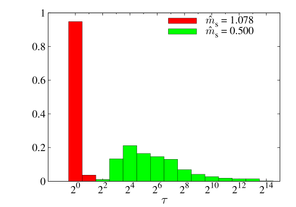
Figure 8: (Color online) Histograms of thermalization times for our $L=32$ simulations, at two values of $\hat{m}_{\mathrm{s}}$ for $\hat{m}=0.12$. Notice the logarithmic scale in the horizontal axis, which is in units of $300$ parallel-tempering steps. The minimum of the effective potential (the peak in the probability distribution) at this $\hat{m}=0.12$ corresponds to $\hat{m}_{\mathrm{s}}=1.078$. Notice that we cannot measure times shorter than our measuring frequency of $300$ parallel-tempering steps, so the first bin should be taken as encompassing all shorter autocorrelation times. Only the samples with $\tau\gtrsim 2^{6}$ have to be extended from the minimum simulation time.

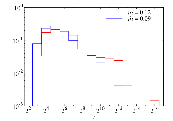
Figure 9: (Color online) Same as Fig. 8, but now we consider several values of $\hat{m}$ for $\hat{m}_{\mathrm{s}}=0.8$ (in the hard thermalization region far from the peak). The points for $\hat{m}=0.12$, closer to the critical point, exhibit a much heavier long-times tail (mind the vertical logarithmic scale).

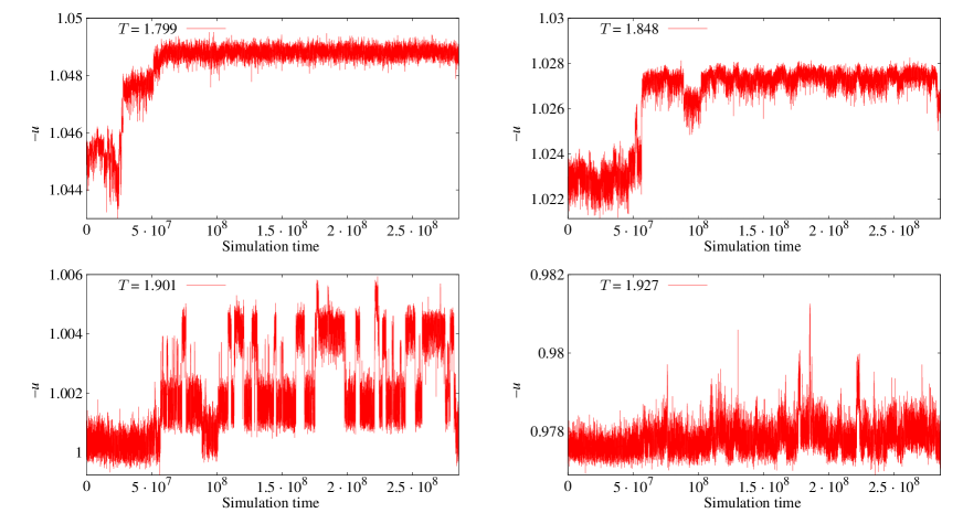
Figure 10: (Color online) Time evolution (in number of parallel tempering steps) for the energy density $u$ for several temperatures of a single $L=32$ sample at $\hat{m}=0.12$, $\hat{m}_{\text{s}}=0.7$. For most temperatures the equilibrium value is quickly reached, but for a very narrow temperature range there are several competing metastable states (bottom-left panel for $T=1.901$).

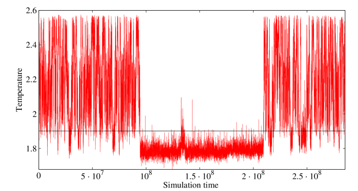
Figure 11: (Color online) Temperature random walk for one of the 40 replicated systems for the parallel tempering simulation of the sample in Figure 10. The flow is blocked at the same temperature that had several metastable states (marked with a horizontal line), see bottom-left panel in Fig. 10.

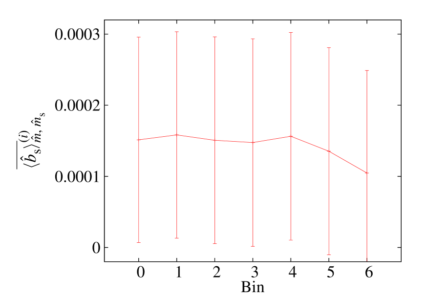
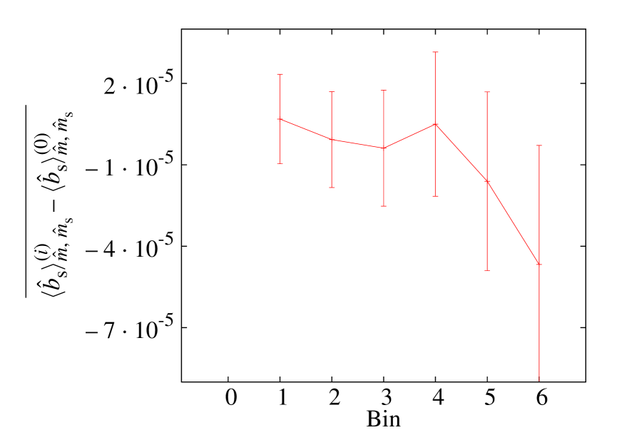
Figure 12: (Color online) Left: Time evolution of $\overline{\langle\hat{b}_{\mathrm{s}}\rangle}_{\hat{m},\hat{m}_{\mathrm{s}}}$ for $\hat{m}=0.12$, $\hat{m}_{\mathrm{s}}=0.5$, in a logarithmic scale (the first bin is the average over the second half of the simulation, the second bin the average over the second quarter and so on). This is in the middle of the $(\hat{m},\hat{m}_{\mathrm{s}})$ region where thermalization is hardest. Right: Same figure, but now subtracting the value of the first bin from each of the following ones. Since the data are correlated, this subtraction causes a very significant error reduction, but the difference is still compatible with zero for several bins.

4.6.1 Optimizing Tethered Monte Carlo simulations

We can highlight two interesting facts from the previous discussion

• Only a very narrow region around the minima of the effective potential has any significant weight for reconstructing canonical averages (Figure 7).

• It is much harder to equilibrate the region far from the minima (Figure 8).

Combining these two observations, it turns out that, if our only interest is reconstructing canonical averages, we can achieve a qualitative improvement in simulation time by simulating only a narrow range around the peak in $P(\hat{m}_{\text{s}}|\hat{m})$ for each value of the smooth magnetization $\hat{m}$. In fact, all the results discussed in fernandez:11b could have been computed in this simplified way, except for the hyperscaling violations exponent $\theta$.

We have demonstrated this optimization by simulating $400$ samples of an $L=48$ system for $\hat{m}=0.12$. We use only $N_{\hat{m}_{\text{s}}}=6$ (but we have to increase the number of temperatures in the parallel-tempering to keep the exchange acceptance high). Table 3 shows the value of $\hat{m}_{\text{s}}^{\text{peak}}$ as a function of $L$.

Table 3: Value of the peak position for our different system sizes. The result for $L=48$ is of comparable accuracy, despite being computed from only $6$ tethered simulations around the minimum of the effective potential. Notice that for $L\leq 32$ we can average over the positive and negative peaks, so the number of samples for these systems is effectively double the value shown in Table 2.

$L$	$N_{\text{samples}}$	$N_{\hat{m}_{\text{s}}}$	$\hat{m}_{\text{s}}^{\text{peak}}-1/2$
8	$1000\times 2$	31	0.58585(87)
12	$1000\times 2$	35	0.58239(54)
16	$1000\times 2$	35	0.58154(36)
24	$1000\times 2$	33	0.57839(24)
32	$700\times 2$	25	0.57672(20)
48	400	6	0.57491(33)

4.7 Geometrical study of the critical configurations

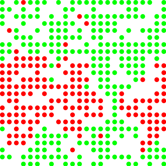
Figure 13: (Color online) Equilibrium configuration for an $L=24$ system at $\beta=0.625$, $\hat{m}=0.12$, $\hat{m}_{\mathrm{s}}=0.5$.

The picture painted in fernandez:11b is that of a second-order transition, but one with quite extreme behavior. Among its peculiarities we can cite an extremely small value of $\beta$ and large free-energy barriers, features both that are reminiscent of first-order behavior. The free-energy barriers in the DAFF, however, diverge too slowly to be associated to the surface tension of well defined, stable coexisting phases. But this only begs the question of what kind of configurations can give rise to such a behavior.

In this section we shall study the geometrical properties of the minimal-cost spin configurations joining the two ordered phases at the critical point. To this end, we consider simulations at $\beta=0.625$, $\hat{m}=0.12\approx\hat{m}_{\mathrm{critical}}$ and $\hat{m}_{\mathrm{s}}=0.5$. Recalling that $\hat{m}_{\mathrm{s}}\simeq m_{\mathrm{s}}+1/2$, this last condition expresses the fact that we are studying configurations with no global staggered magnetization. This is a good example of an ‘inherently tethered’ study, that examines information hidden from a canonical treatment.

Figure 13 shows an example of such a configuration for an $L=24$ system. In order to make the different phases clearer, we are not representing the spin field $s_{\boldsymbol{x}}$, but the staggered field $s_{\boldsymbol{x}}\pi_{\boldsymbol{x}}$. As is readily seen, even if the global magnetization is $m_{\mathrm{s}}\approx 0$, the system is divided into two phases with opposite (staggered) spin. In geometrical terms, most of the occupied nodes of the system belong to one of two large clusters with opposite sign, with only a few scattered smaller clusters.

At a first glance, this picture may seem consistent with a first-order scenario, were the system is divided into two strips whose surface tension gives rise to the free-energy barriers (see martin-mayor:07 for an example of these geometrical transitions in a first-order setting). In order to test this possibility, we can study the evolution of the interface mass with the system size and compare it with the explicit computation of free-energy barriers done in fernandez:11b .

Given a configuration, we first trace all the geometric antiferromagnetic clusters. We then identify the largest and second largest ones. Finally, we say that an occupied node belongs to the ‘interface’ if it belongs to the largest cluster and has at least one first neighbor belonging to the second largest one. We have computed in this way the interface $N_{\mathrm{interface}}$ for our $700$ $L=32$ samples and for $3000$ samples for all our smaller systems (we have run additional simulations just at this point). Table 4 shows the result of this computation. A fit to

$$N_{\mathrm{interface}}=AL^{c},$$ (65)

for $L\geq 12$ gives $c=2.2402(24)$ with $\chi^{2}/$d.o.f. $=3.62/2$. One may think that such a large exponent could be indicative of a surface tension. However, the study of fernandez:11b showed that free-energy barriers in the DAFF grow as $L^{\theta}$, with $\theta=1.469(20)\neq c$. Indeed, for the archetypical second-order model, the $D$-dimensional pure Ising ferromagnet, the percolating clusters are space filling, so $c=D$.

Table 4: Masses of the interfaces for our equilibrium spin configurations at $\beta=0.625$, $\hat{m}=0.12\approx\hat{m}_{\mathrm{c}}$, $\hat{m}_{\mathrm{s}}=0.5$. This mass grows as $N_{\mathrm{interface}}\propto L^{c}$. From a fit, $c=2.2402(24)$, which is incompatible with our estimate of $\theta=1.469(20)$, confirming that the free-energy barriers are not associated to surface tensions.

$L$	$N_{\mathrm{samples}}$	$N_{\mathrm{interface}}$
12	3000	160.29(25)
16	3000	304.62(41)
24	3000	755.74(94)
32	700	1446.1(39)1

A second interesting feature of the configuration pictured on Figure 13 is that there is a path connecting the spins in the green strip across the red one (there is only one green strip, since we are considering periodic boundary conditions). If we were to study a complete tomography of this configuration, we would find several of these paths (which, of course, need not be contained in a plane). In other words, the phases are porous. This is in clear contrast to a first-order scenario in which the phases are essentially impenetrable walls. Now, this could be a peculiarity of the particular selected configuration. In order to make the analysis quantitative, we shall examine all of our samples and determine the strip-crossing probability $P$. This is defined as the probability of finding a complete path with constant staggered spin across the strip with opposite staggered magnetization and we can compute it with the following algorithm:

1. For each configuration, compute the Fourier transform of the staggered spin field at the smallest nonzero momentum in each of the three axes ($\phi_{x}$, $\phi_{y}$, $\phi_{z}$).

2. If the system is in a strip configuration, one of the $\phi$ will be much larger than the other two. Assume this is $\phi_{x}$, so the strips are perpendicular to the $OX$ axis.

3. Measure the staggered magnetization $M_{\mathrm{s}}^{x}$ on each of the planes with constant $x$ and identify the plane $x=x_{\mathrm{max}}$ with largest $|M_{\mathrm{s}}^{x}|$. This plane will be at the core of one the strips.

4. Trace all the clusters that contain at least one spin on the $x=x_{\mathrm{max}}$ plane, but severing the links between planes $x=x_{\mathrm{max}}$ and $x=x_{\mathrm{max}}-1$.

5. If any of the clusters reaches the plane $x=x_{\mathrm{max}}-1$ there is at least a path through the strip with opposite magnetization (the previous step has forced us to go the long way around, so we know we have crossed the strip).

We have plotted the strip-crossing probability $P$ as a function of $\hat{m}$ in Figure 14. Notice that $1-P$ behaves as an order parameter. If we keep increasing $\hat{m}$, so that we enter the ordered phase, the phases eventually become proper impenetrable strips, hence $P=0$ for large enough systems. On the other hand, for low $\hat{m}$, in the disordered phase, the strips become increasingly porous, so that $P=1$ in the limit of large systems. In fact, the inversion of the finite-size evolution at $\hat{m}\approx 0.12$ signals the onset of the phase transition.

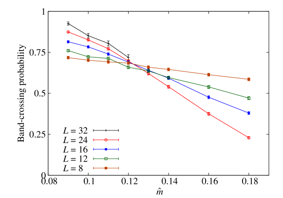
Figure 14: (Color online) Probability of completing a path with constant staggered spin across the strip with opposite staggered magnetization, see Fig. 13, for our spin configurations at $\beta=0.625$, $\hat{m}_{\mathrm{s}}=0.5$.

5 Hard Spheres Crystallization

In this Section we consider a completely different problem, namely hard-spheres crystallization, as an illustration of the flexibility of the Tethered Monte Carlo. In particular, this problem has neither quenched disorder, nor a supporting lattice. Furthermore, the phase transition is of the first-order, rather than continuous.

Actually, crystallization (or melting) is probably the most familiar example of a first order transition. Most fluids undergo a transition to a crystalline solid upon cooling or compression. One might thus be shocked to learn that a bona-fide Monte Carlo simulation of crystallization, conforming to the standards taught in good textbooks sokal:97 , is plainly impossible nowadays.

The problem is that there are simply too many local minima of the effective potential where the simulation can get trapped. Some degree of cheating (you could also say artistry) is needed to guide the simulation.

That the problem is a fairly subtle one is illustrated by the fact that hard-spheres crystallize in three dimensions alder:57 ; wood:57 , even if the fluid and the face-centered cubic (FCC) crystals have exactly the same energy. In fact, hard spheres have become the standard model in the field, where all new ideas must be tested. Besides their theoretical interest, hard spheres provide as well an important model for colloidal suspensions pusey:86 ; pusey:89 .

In fact, workable numerical methods vega:08 put by hand the crystal in the simulation. One may try to achieve equilibrium between the crystal and the fluid, as in the phase switch Monte Carlo wilding:00 , but this is feasible only for small systems (up to $N=500$ hard spheres errington:04 ). One may also compute separately the fluid and solid free energies. For the fluid, one resorts to thermodynamic integration, while several methods are available for the crystal (Wigner-Seitz hoover:68 , Einstein crystal frenkel:84 ; polson:00 , Einstein molecule vega:07 ). The transition point is determined by imposing to both phases the conditions of equal pressure, temperature and chemical potential. An alternative is direct coexistence ladd:77 ; noya:08 , a dynamic, non-equilibrium method that simulates rather large systems with great accuracy zykova-timan:10 .

Our scope here is to illustrate how Tethered Monte Carlo can be used in this context. Indeed, it has been recently shown that Tethered Monte Carlo allows equilibrating up to $N=2916$ hard spheres at their phase coexistence pressure fernandez:11 . As explained in the Introduction, constrained Monte Carlo studies of crystallization kinetics have been carried out before tenwolde:95 ; chopra:06 , in an umbrella sampling framework.

The remaining part of this section is organized as follows. In Sect. 5.1 we recall the hard sphere model. Our order parameters are defined in Sect. 5.2. The specific implementation of the tethered formalism is in Sect. 5.3. Details about the computation of the phase-coexistence pressure fernandez:11 are provided in Sects. 5.4 and 5.5. The performance of the Tethered Monte Carlo algorithm is assessed in 5.6. Finally, we comment on the computation of the interfacial free energy in Sect. 5.7.

5.1 The hard spheres model

We consider a collection of $N$ hard spheres, of diameter $\sigma$. They are contained in a cubic simulation box, with periodic boundary conditions. The system is held at constant pressure $p$ (hence the simulation box may change its volume, but remaining always cubic).

Let us introduce the shorthand $\boldsymbol{R}$ for the set of particle positions, $\{\boldsymbol{r}_{i}\}_{i=1}^{N}$. The constraint of no overlapping spheres is expressed with function $H(\boldsymbol{R})$, which vanishes if any pair of spheres overlaps ($H(\boldsymbol{R})=1$ otherwise).

The Gibbs free-energy density, $g(p,T)$, is obtained from the partition function

$$Y_{NpT}=\mathrm{e}^{-N\beta g(p,T)}=\frac{p\beta}{N!\Lambda^{3N}}\int_{0}^{\infty}\mathrm{d}V\mathrm{e}^{-\beta pV}\int\mathrm{d}\boldsymbol{R}\,H(\boldsymbol{R})\,,$$ (66)

where $\Lambda$ is the de Broglie thermal wavelength, while $\beta=1/(k_{\mathrm{B}}T)$.

5.2 The two order parameters

The standard order parameter for modern crystallization studies is $Q_{6}$ steinhardt:83 ; duijneveldt:92 , which is the $l=6$ instance of

$$Q_{l}\equiv\left(\frac{4\pi}{2l+1}\sum_{m=-l}^{l}\left|Q_{lm}\right|^{2}\right)^{1/2}\,,$$ (67)

where

$$Q_{lm}\equiv\frac{\sum_{i=1}^{N}\,q_{lm}(i)}{\sum_{i=1}^{N}N_{b}(i)}\,,\quad q_{lm}(i)\equiv\sum_{j=1}^{N_{b}(i)}Y_{lm}({\hat{\boldsymbol{r}}_{ij}})\,.$$ (68)

In the above expression, $Y_{lm}(\hat{\boldsymbol{r}}_{ij})$ are the spherical harmonics, while $\hat{\boldsymbol{r}}_{ij}$ is the unit vector in the direction joining particles $i$ and $j$, $\boldsymbol{r_{ij}}=\boldsymbol{r}_{i}-\boldsymbol{r}_{j}$. $N_{b}(i)$ represents the number of neighbors of the $i$th particle. It is important to note that, setting aside the periodic boundary conditions for our simulation box, $Q_{6}$ is rotationally invariant. $Q_{6}$ is of order $1/\sqrt{N}$ in a fluid phase, whereas $Q_{6}\approx 0.574$ or $0.510$ in perfect FCC or BCC crystals, respectively. However, defective crystals have lesser values ($Q_{6}\approx 0.4$ is fairly common).

Now, if one tries to perform a tethered computation, choosing $Q_{6}$ as order parameter, it is soon discovered that it is almost impossible to form an FCC crystal if the starting particle configuration is disordered. Instead, the simulation gets stuck in helicoidal crystals, with a similar value of $Q_{6}$, which are allowed by the periodic boundary conditions. The crystalline planes for these helicoidal structures are misaligned with the simulation box. Upon reflection, one realizes that the problem lies in the rotational invariance of $Q_{6}$. When a crystalline grain starts to nucleate from the fluid, which is encouraged by the tethered algorithm for large $\hat{Q}_{6}$, we face the problem that $Q_{6}$ conveys no information about the relative orientation of the growing grain with respect to the simulation box. At some point, the misaligned crystalline grain is large enough to hit itself through the periodic boundary conditions, and it needs to contort to get some matching for the crystalline planes.

The way out is in an order parameter with only cubic symmetry. Such a parameter was recently proposed angioletti:10 :

$$C=\frac{2288}{79}\frac{\sum_{i=1}^{N}\sum_{j=1}^{N_{b}(i)}c_{\alpha}({\hat{\boldsymbol{r}}_{ij}})}{\sum_{i=1}^{N}N_{b}(i)}-\frac{64}{79}\,,$$ (69)

where

$$c_{\alpha}(\hat{\boldsymbol{r}})=x^{4}y^{4}(1-z^{4})+x^{4}z^{4}(1-y^{4})+y^{4}z^{4}(1-x^{4})\,.$$ (70)

The expectation value for $C$ in the different phases is the following: $0.0$ in the fluid, $1.0$ in the ideal FCC crystal, perfectly aligned with the simulation box, and $-0.26$ in the perfectly aligned ideal BCC. The difference with the quoted value in Ref. angioletti:10 for the perfect BCC crystal is due to our smaller threshold for neighboring particles. Again, as it happens for $Q_{6}$, we must expect lower $|C|$ values for defective structures.

In fact, we find that tethered simulations with a single order parameter ($C$) and large $\hat{C}$, equilibrate easily. One forms nice crystals even if the starting particle configuration is disordered, and the Monte Carlo expectation values turn out to be independent of the starting configuration, as they should.

However, not all is well. At some intermediate values of $\hat{C}$ the simulation suffers from metastabilities. Heterogeneous states with a slab of FCC crystal in a fluid matrix are degenerate with helicoidal crystals, that fill most of the simulation box, but have a small value of $C$ because of their misalignment. Fortunately, these two types of competing configurations are clearly differentiated by $Q_{6}$, which is large for the helicoidal crystal, but small for the crystalline slab surrounded by fluid. Therefore, the combination of the two order parameters labels unambiguously the intermediate states between the fluid and the FCC crystal.

5.3 Tethered formalism for a hard sphere system

Since we wish to constraint simultaneously the two crystal order parameters, $\hat{Q}_{6}$ and $\hat{C}$, we use the formalism in Sect. 3.1. We choose to couple the demons linearly, which frees us from the constraints $\hat{Q}_{6}>Q_{6}(\boldsymbol{R})$ and $\hat{C}>C(\boldsymbol{R})$ imposed by quadratic demons. Note that ascertaining thermalization is an issue in crystallization studies. It is very important to compare the outcome of simulations with widely differing starting configurations. In this respect, the constraints $\hat{Q}_{6}>Q_{6}(\boldsymbol{R})$ and $\hat{C}>C(\boldsymbol{R})$ are a major problem, as they prevent us from using the ideal FCC crystal as starting configuration.

As for the tunable parameter $\alpha$, see Eq. (37), we choose $\alpha=200$. In this way, the convolution in the probability distribution functions induced by the demons does not result into a gross distortion.

Our tethered statistical weight is

$$\omega_{N}(\boldsymbol{R},V;p,\hat{Q}_{6},\hat{C})=\frac{N\alpha}{2\pi}H(\boldsymbol{R})\ {\mathrm{e}}^{-\beta pV-N\alpha\,\left[{\left({\hat{Q_{6}}-Q_{6}(\boldsymbol{R})}\right)^{2}+\left({\hat{C}-C(\boldsymbol{R})}\right)^{2}}\right]/2}\,.$$ (71)

As follows from Eq. (38), the gradient of the Helmholtz effective potential is

$$\boldsymbol{\nabla}{\varOmega_{N}(\hat{Q}_{6},\hat{C},p)}=\left({\frac{\partial\varOmega_{N}(\hat{Q}_{6},\hat{C})}{\partial\hat{Q}_{6}},\frac{\partial\varOmega_{N}(\hat{Q}_{6},\hat{C})}{\partial\hat{C}}}\right)=\left({\bigl{\langle}\hat{b}_{Q_{6}}\bigr{\rangle}_{\hat{Q}_{6},\hat{C},p},\bigl{\langle}\hat{b}_{C}\bigr{\rangle}_{\hat{Q}_{6},\hat{C},p}}\right),$$ (72)

with

$$\hat{b}_{Q_{6}} =\alpha\left({\hat{Q}_{6}-Q_{6}}\right), \hat{b}_{C} =\alpha\left({\hat{C}-C}\right).$$ (73)

The relationship between the effective potential, $\Omega_{N}(\hat{Q}_{6},\hat{C},p)$, and the Gibbs free-energy density is straightforward:

$$Y_{NpT}=e^{-Ng_{N}(p,T)}=\int\mathrm{d}\hat{Q}_{6}\ \mathrm{d}\hat{C}\ e^{-N\varOmega_{N}(\hat{Q}_{6},\hat{C},p)}\,.$$ (74)

Furthermore, a saddle-point approximation, see Sect. 3.2, shows that

$$g_{N}(p,T)=\varOmega_{N}(\hat{Q}_{6}^{*},\hat{C}^{*},p)+O(1/N)\,,$$ (75)

where $(\hat{Q}_{6}^{*},\hat{C}^{*},p)$ corresponds to the $p$-dependent absolute minimum of $\varOmega_{N}(\hat{Q}_{6},\hat{C},p)$, regarded as a function of $\hat{Q}_{6}$ and $\hat{C}$. However, it is important to keep in mind that near the phase transition two local minima (namely the fluid and the FCC crystal) become exactly degenerate.

5.4 The coexistence pressure: computing differences in the effective potential

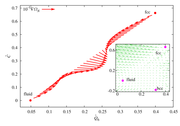
Figure 15: (Color online) $\boldsymbol{\nabla}\varOmega_{N=256}$, as computed from Eq. (73) for $N=256$ hard spheres, along the straight path that joins the fluid and the FCC minima of the effective potential. The simulation pressure is the phase-coexistence one. To improve visibility, we have divided $\boldsymbol{\nabla}\varOmega_{N=256}$ by a factor of 10. Inset: map of the gradient field $\boldsymbol{\nabla}\varOmega_{N=256}$, including the points corresponding to the fluid, FCC and BCC potential minima. For the sake of visibility we have divided the gradient by a factor $\alpha=200$ (mind the different normalization as compared with main panel).

The coexistence pressure, $p_{\mathrm{co}}$, follows from the difference in effective potential between the pressure-dependent coordinates of the coexisting pure phases:

$$\Delta\Omega_{N}(p)=\Omega_{N}\bigl{(}\hat{Q}_{6}^{\mathrm{FCC}}(p),\hat{C}^{\mathrm{FCC}}(p),p\bigr{)}-\Omega_{N}\bigl{(}\hat{Q}_{6}^{\mathrm{fluid}}(p),\hat{C}^{\mathrm{fluid}}(p),p\bigr{)}\,.$$ (76)

The scope of the game is finding the coexistence pressure, $p_{\mathrm{co}}^{N}$, such that $\Delta\Omega_{N}(p_{\mathrm{co}}^{N})=0$. Indeed, the saddle-point condition (75), tells us that, at $p_{\mathrm{co}}^{N}$, the chemical potential for the two phases coincides.

Now, the computation of $\Delta\Omega_{N}(p)$ is strictly analogous to that of section 4.3. We obtain the difference in the effective potential as a line integral of the conservative field $\hat{\boldsymbol{B}}$. The most convenient path is a straight line, see Fig. 15. As in Sect. 4.3, we divide the path in a mesh, perform independent simulations at each point of the grid, and compute $\Delta\Omega_{N}(p)$ from a numerical integration of the gradient, Eq. (72), projected over the path.

Let us stress only the main difference with the computation in Sect. 4.3:

• Here, we wish to compute $\Delta\Omega_{N}(p)$ as a function of pressure. Instead, in section 4.3 we were restricted to a single value of the control parameter (temperature in that case).

• The disorder-averaging procedure introduced in Sect. 4.4 dispensed us from a careful search of local minima. Instead, locating with very high accuracy the extremal points $\bigl{(}\hat{Q}_{6}^{\mathrm{FCC}}(p),\hat{C}^{\mathrm{FCC}}(p)\bigr{)}$ and $\bigl{(}\hat{Q}_{6}^{\mathrm{fluid}}(p),\hat{C}^{\mathrm{fluid}}(p)\bigr{)}$ is a must here, see Sect. 5.5.

• The choice of a straight line as integration path, see Fig. 15, is not only dictated by simplicity. It is also a matter of computational convenience. Thermalization is easier to achieve over it. Furthermore, as the gradient map in the inset of Fig. 15 shows, the gradient takes its smallest absolute value over this path.

In order to compute $p_{\mathrm{co}}^{N}$, let us neglect the pressure dependence of the end points for the integration path in Fig. 15. One may easily correct for end-points displacements, as explained in Sect. 5.5, which induces a correction in $p_{\mathrm{co}}^{N}$ negligible with respect to our statistical errors.

Under the above simplifying assumption, we only need the pressure dependence of the gradient field, $\hat{\boldsymbol{B}}$, over the straight path in Fig. 15. Using histogram reweighting falcioni:82 ; ferrenberg:88 , we extrapolate our numerical results at pressure $p$ to a neighboring $p+\delta p$:

$$\langle\hat{\boldsymbol{B}}\rangle_{\hat{Q}_{6},\hat{C},p+\delta p}=\frac{\langle\hat{\boldsymbol{B}}\mathrm{e}^{-\delta pV}\rangle_{\hat{Q}_{6},\hat{C},p}}{\langle\mathrm{e}^{-\delta pV}\rangle_{\hat{Q}_{6},\hat{C},p}}.$$ (77)

A standard argument tells us that the maximum safe extrapolation, $\delta p$, is determined by the probability distribution function (pdf) for the specific-volume, $v=V/N$,

$$\delta p^{\mathrm{maximum}}\approx\frac{1}{\sqrt{N\chi_{p}}}\,,\quad\chi_{p}=\left.\frac{\partial\langle v\rangle}{\partial p}\right|_{(\hat{Q}_{6},\hat{C},p)}=N\bigl{[}\langle v^{2}\rangle_{\hat{Q}_{6},\hat{C},p}-\langle v\rangle^{2}_{\hat{Q}_{6},\hat{C},p}\bigr{]}\,.$$ (78)

Hence, it is crucial that the pdf for $v$ be unimodal (i.e. single-peaked), and with an $N$-independent $\chi_{p}$, for all point along the integration path. In other words, it is important that the integration path be free of metastabilities. Since this condition holds seoane:12 , it is straightforward to compute $\Delta\Omega_{N}(p+\delta p)$ from simulations at $p$.

Following these guidelines, $p_{\mathrm{co}}^{N}$ was computed in Ref. fernandez:11 for $108\leq N\leq 2916$. The large $N$ extrapolation was

$p_{\mathrm{co}}^{\infty}=11.5727(10)$ fernandez:11  .

The best previous equilibrium estimate seems to be the rather crude $p_{\mathrm{co}}^{\infty}=11.50(9)$ wilding:00 , obtained using phase-switch Monte Carlo. In fact, the only previous method accurate enough to provide a meaningful comparison is the non-equilibrium direct-coexistence: $p_{\mathrm{co}}^{\infty}=11.576(6)$ zykova-timan:10 . Note, however, that in order to achieve such a small error (but still six times larger than the tethered error), systems with up to $N=1.6\times 10^{5}$ particles were simulated zykova-timan:10 .

5.5 Calculation of the extremal points and corrections

We need to locate the two extremal points in the straight path in Fig. 15, which correspond to the fluid or to the FCC crystal. The two points are local minima of $\Omega_{N}$, regarded as a function of $\hat{Q}_{6}$ and $\hat{C}$ but at fixed pressure. Our procedure has been as follows.

We first obtain a crude estimate from standard simulations in the $NpT$ ensemble (without any constrain in the crystal parameters). Note that the autocorrelation time for such simulations is unknown, but larger than any simulation performed to date. Hence, these standard simulations get stuck at the local minimum of $\Omega_{N}$ which is most similar to their starting configuration. Starting the simulation either from an ideal gas, or from a perfect FCC crystal, we approach the pure-phases we are interested in. The Monte Carlo average of $Q_{6}(\boldsymbol{R})$ and $C(\boldsymbol{R})$ provides our first guess.

To refine the search of either of the two local minima $(\hat{Q}_{6}^{*},\hat{C}^{*})$, we note that, up to terms of third order in $\hat{Q}_{6}-\hat{Q}_{6}^{*}$ or $\hat{C}-\hat{C}^{*}$,

$$\Omega_{N}(\hat{Q}_{6},\hat{C})=\Omega_{N}^{*}+\frac{A_{QQ}}{2}(\hat{Q}_{6}-\hat{Q}_{6}^{*})^{2}+A_{QC}(\hat{Q}_{6}-\hat{Q}_{6}^{*})(\hat{C}-\hat{C}^{*})+\frac{A_{CC}}{2}(\hat{C}-\hat{C}^{*})^{2}\,.$$ (79)

The shorthand $\Omega_{N}^{*}$ stands for $\Omega_{N}(\hat{Q}_{6}^{*},\hat{C}^{*})$. Incidentally, Eq. (79) tells us that the computation in Sect. 5.4 is intrinsically stable. An error of order $\epsilon$ in the location of $(\hat{Q}_{6}^{*},\hat{C}^{*})$ will result in an error of order $\epsilon^{2}$ in the coexistence pressure.

Yet, the tethered computation does not give us access to $\Omega_{N}$, but to its gradient:

$$\boldsymbol{\nabla}\Omega_{N}(\hat{Q}_{6},\hat{C})=\bigl{(}A_{QQ}(\hat{Q}_{6}-\hat{Q}_{6}^{*})+A_{QC}(\hat{C}-\hat{C}^{*}),A_{CC}(\hat{C}-\hat{C}^{*})+A_{QC}(\hat{Q}_{6}-\hat{Q}_{6}^{*})\bigr{)}\,.$$ (80)

Eq. (80) holds up to corrections quadratic in $\hat{Q}_{6}-\hat{Q}_{6}^{*}$ or $\hat{C}-\hat{C}^{*}$. We thus compute the expectation value of the field $\hat{\boldsymbol{B}}$, in a grid of nine points $(\hat{Q}_{6},\hat{C})$ that surround our first guess for $(\hat{Q}_{6}^{*},\hat{C}^{*})$, and fit the results to Eq. (80). We iterate this procedure until an accuracy $\sim 10^{-6}$ in both coordinates $(\hat{Q}_{6}^{*},\hat{C}^{*})$ is reached seoane:12 .

Actually, Eq. (77), shows how one extrapolates the expectation values for the gradient field from the simulated pressure, $p$ to a nearby $p+\delta p$. The corresponding fit to Eq. (80) provides the new coordinates $\bigl{(}\hat{Q}_{6}^{*}(p+\delta p),\hat{C}^{*}(p+\delta p)\bigr{)}$.

At this point, one could worry because the integration path in Fig. 15 is no longer appropriate at pressure $p+\delta p$. In fact, the extremal points in the integration path are pressure-dependent. However, some reflection shows that this is not a real problem. In fact,

$$\Delta\Omega_{N}(p+\delta p)=\Delta^{\mathrm{FCC}}(p,p+\delta p)+\Delta^{\mathrm{path}}(p,p+\delta p)-\Delta^{\mathrm{fluid}}(p,p+\delta p)\,.$$ (81)

The different pieces are

$$\Delta^{\mathrm{FCC}}(p,p+\delta p) = \Omega_{N}\bigl{(}\hat{Q}_{6}^{\mathrm{FCC}}(p+\delta p),\hat{C}^{\mathrm{FCC}}(p+\delta p);\,p+\delta p\bigr{)}-$$

$$- \Omega_{N}\bigl{(}\hat{Q}_{6}^{\mathrm{FCC}}(p),\hat{C}^{\mathrm{FCC}}(p);\,p+\delta p\bigr{)}\,,$$

the correction due to the shift of order $\delta p$ in the coordinates of the FCC minimum,

$$\Delta^{\mathrm{path}}(p,p+\delta p) = \Omega_{N}\bigl{(}\hat{Q}_{6}^{\mathrm{FCC}}(p),\hat{C}^{\mathrm{FCC}}(p);\,p+\delta p\bigr{)}-$$

$$- \Omega_{N}\bigl{(}\hat{Q}_{6}^{\mathrm{fluid}}(p),\hat{C}^{\mathrm{fluid}}(p);\,p+\delta p\bigr{)}\,,$$

the line-integral sketched in Fig. 15 as computed at pressure $p+\delta p$, and

$$\Delta^{\mathrm{fluid}}(p,p+\delta p) = \Omega_{N}\bigl{(}\hat{Q}_{6}^{\mathrm{fluid}}(p+\delta p),\hat{C}^{\mathrm{fluid}}(p+\delta p);\,p+\delta p\bigr{)}-$$

$$- \Omega_{N}\bigl{(}\hat{Q}_{6}^{\mathrm{fluid}}(p),\hat{C}^{\mathrm{fluid}}(p);\,p+\delta p\bigr{)}\,,$$

the correction due to the shift in the coordinates of the fluid minimum.

Now, one expects that the pressure-induced changes in the minima coordinates as well as on the coefficients $A_{QQ}$, $A_{Q,C}$ and $A_{CC}$ will of order $\delta p$. Hence, Eq. 79 implies that both $\Delta^{\mathrm{FCC}}(p,p+\delta p)$ and $\Delta^{\mathrm{fluid}}(p,p+\delta p)$ are of order $(\delta p)^{2}$. This is the rationale behind the simplifying assumption made in Sect. 5.4.

At any rate, $\Delta^{\mathrm{FCC}}(p,p+\delta p)$ and $\Delta^{\mathrm{fluid}}(p,p+\delta p)$ can be numerically computed from Eq. 79. For all values of $N$ simulated in Ref. fernandez:11 , their combined effect on the determination of the coexistence pressure turns out to be smaller than 1% of the statistical error bars seoane:12 .

5.6 Algorithmic performance

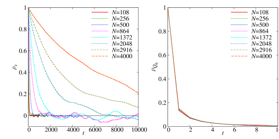
Figure 16: (Color online) Normalized time autocorrelation function, Eq. 87, for the specific volume (left) and the crystal order parameter (right), as computed for a system of $N$ hard spheres, in the fluid minimum of the effective potential (labeled $S=0$). Time is measured in units of EMCS (see text). Mind the different time scale for the left and right panels. Each value of $N$ was simulated very close to (but not precisely at) its phase-coexistence pressure $p_{\mathrm{co}}^{N}$ fernandez:11 .

The simulation of the weight in Eq. (71) requires two types of moves: single particle displacements, as well as changes in the volume of the simulation box. We shall use the short hand Elementary Monte Carlo Step (EMCS) to the combination of $N$ consecutive single-particle displacements attempts, followed by a change attempt in the simulation box volume.

The standard tools to asses the performance of a Monte Carlo algorithm sokal:97 are briefly recalled in the Appendix A.

Recall that we will be discussing independent simulations along the path in Fig. 15. We thus will be labeling them by means of a coordinate $S$, such that $S=0$ corresponds to the fluid pure phase, while $S=1$ refers to the FCC minimum.

One should like to consider the time autocorrelation functions for the components of the gradient field, $\hat{b}_{Q_{6}}$ and $\hat{b}_{C}$. Yet, Eq. (73) tells us that these correlation functions are identical to those of $Q_{6}(\boldsymbol{R})$ and $C(\boldsymbol{R})$. Eq. (77) suggests as well that the time autocorrelation function for the specific volume $v$ is of interest. An example of these autocorrelation functions is shown in Fig. 16, for the $S=0$ point. We note that $v$ plays the role of the algorithmic slow mode, with a strong $N$ dependence. On the other hand, the autocorrelation function for $Q_{6}$ decreases very fast, and it is barely $N$-dependent. The autocorrelation function for $C$ is qualitatively identical to that of $Q_{6}$, and will thus be skipped.

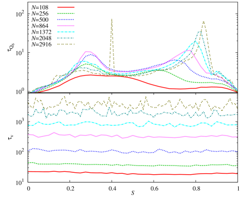
Figure 17: (Color online) Integrated autocorrelation times, defined in Eq. 88, for $Q_{6}$ (top) and $v$ (bottom), as a function of $S$ (the linear coordinate that labels the integration path in Fig. 15, where $S=0$ stands for the fluid minimum and $S=1$ represents the homogeneous FCC phase). Time is measured in units of EMCS. Results for all values of $N$ equilibrated in Ref. fernandez:11 .

The analysis is made quantitative by considering the integrated autocorrelation times, see Fig. 17. We notice that the dynamics of $v$ is considerable slower than that of $Q_{6}$, and featureless as a function of $S$. Data for the specific volume scales as $\tau_{v}\sim N^{5/3}$ (quite worse than standard critical slowing down in three dimensions, $\tau\sim N^{2/3}$, yet much better than exponential dynamic slowing-down). There is a clear anomaly in the behavior of $\tau$ for a single simulation point in $N=2916$. We briefly comment on this below.

Using these tools, it was ensured in Ref. fernandez:11 that all simulations were, at least, $50\tau$ long. Besides, all simulations were performed twice, with different starting configurations (either an ideal FCC crystal, or an ideal gas). Compatibility between the two sets of investigations was systematically checked seoane:12 .

The anomaly at $S=0.4$ for $N=2916$ is due to the emergence of metastability. At this value of $S$ we expected to find a spatially segregated state (a slab of FCC crystal in a liquid matrix). This state appeared indeed, but the simulation tunnels back and forth from it to an helicoidal crystal (in close analogy with the Monte Carlo history shown in the bottom-left panel of Fig. 10). We actually performed extra simulations in this point, in order to determine the relative weight of each of the two metastable states (their effect was carefully considered in final estimates seoane:12 ).

These helicoidal crystals appear much more often for $N=4000$ and intermediate $S$. Nevertheless, selecting carefully the starting particle configuration for the simulation at each $S$, one may obtain a gradient field with a smooth $S$-dependency. However, it is clear that these $N=4000$ results, although plausible, cannot be regarded as well equilibrated fernandez:11 .

5.7 Interfacial free-energy

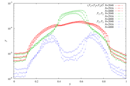
Figure 18: (Color online) For systems of $N$ hard spheres at their phase-coexistence pressure, we show, as a function of the line parameter $S$, different linear combinations of the particle-density fluctuations, Eq. (85), computed for the minimal wavevectors allowed by periodic boundary conditions and ordered in such a way that ${\cal F}_{1}>{\cal F}_{2}>{\cal F}_{3}$. For the phase-separated states all three ${\cal F}$ are of order $1$ (order $1/N$ for homogeneous systems). The slab phase is the only one with ${\cal F}_{1}-{\cal F}_{2}$ of order one. The cylinder phase is identified by ${\cal F}_{2}-{\cal F}_{3}$ of order one.

The interfacial free energy is the free-energy cost per unit area of a liquid-to-crystal interface. Its computation has been rather difficult for hard spheres, different authors finding mutually incompatible results davidchack:00 ; mu:05 ; davidchack:10 .

The tethered formalism allows as well to compute the interfacial free energy fernandez:11 . One should identify a point along the straight path in Fig 15 where a slab of fluid surrounded by an FCC crystal is formed. Such configurations have two phase-separating surfaces of linear dimensions comparable with those of the simulation box. The effective potential difference between such a heterogeneous state and either of the two pure phases provides an estimate of the interfacial free energy. It turns out that a well formed surface appears only for $N\geq 2048$ fernandez:11 . Let us see how this can be ascertained.

The physical situation is as follows. When we go from the liquid to the solid, Fig. 15, the homogeneous fluid becomes unstable at a value of the linear coordinate $S\propto N^{-1/(D+1)}$, which means that a macroscopic droplet of crystal forms. This has been established for all types of first-order phase transitions biskup:02 ; binder:03 ; macdowell:04 ; nussbaumer:06 , and explicitly verified for crystallization fernandez:11 . As $S$ grows the mass of the crystal droplet increases, which costs surface energy. At a certain point, the periodic boundary conditions allow reducing the surface energy by turning the crystal droplet onto a crystal cylinder. At still larger $S$, the cylinder becomes a slab. Of course another three analogous geometrical transitions arise when $S$ keeps increasing as we approach the FCC minimum. All six geometric transitions appeared in large enough hard-spheres systems fernandez:11 . We are interested in identifying systems large enough to form a slab of crystal surrounded by fluid.

To follow these geometric transitions we consider the particle-density fluctuations quantified through

$${\cal F}(\boldsymbol{q})=\frac{1}{N^{2}}\biggl{|}\sum_{i=1}^{N}e^{\mathrm{i}\boldsymbol{q}\cdot\boldsymbol{r}_{i}}\biggr{|}^{2}\,,$$ (85)

As we are interested in the largest wavelength, we consider the smallest $\boldsymbol{q}$ allowed by periodic boundary conditions, $\|\boldsymbol{q}\|=2\pi/L$, where $L$ is the linear size of the simulation box. There are three such minimal wavevectors in a cubic box. Given a particle configuration, ${\cal F}_{1}$ is the maximum over the three directions, ${\cal F}_{3}$ is the minimum, and ${\cal F}_{2}$ is the intermediate one. As the droplet, cylinder and slab geometries have different symmetries the natural order parameters are

• Whenever the system is phase separated, $(\mathcal{F}_{1}+\mathcal{F}_{2}+\mathcal{F}_{3})/3$ is of order 1, (order $1/N$ otherwise).

• For a cylinder, two of the ${\cal F}$’s are of order 1, while the ${\cal F}$ along the cylinder axis is small. Hence, $\mathcal{F}_{2}-\mathcal{F}_{3}$ is of order 1 in the cylinder phase, but it vanishes (for large $N$) both in the droplet and the slab phase.

• For a slab the only ${\cal F}$ of order 1 is that transversal to it. Hence $\mathcal{F}_{1}-\mathcal{F}_{2}$ is of order 1 for a slab, but not for the cylinder nor the droplet.

All these behaviors are identified in Fig. 18. We thus conclude that $N\geq 2048$ is sufficient to attempt a computation of the interfacial free-energy.

To improve the numerical stability, we consider the potential difference between two points, $S^{*}\approx 0.5$ and $S=1$. For both $S$ values, the gradient of $\Omega_{N}$ is normal to the straight in Fig 15 (actually $S=1$ is a local minimum of $\Omega_{N}$, while $S^{*}$ is a local maximum if we restrict ourselves to the straight). Hence, the interfacial free-energy for the $(100)$ crystal direction, $\gamma_{100}$, follows from fernandez:11

$$\frac{\gamma_{100}}{k_{\mathrm{B}}T}=N^{1/3}\frac{\left({\Omega_{\text{FCC}}-\Omega_{S^{*}}}\right)}{2\left\langle{v}\right\rangle_{S^{*}}^{2/3}}\,.$$ (86)

A peculiarity of the tethered approach is that one may control the dependence of the estimate of $\gamma_{100}$ on the actual estimate used for the coexistence pressure. One simply computes $\gamma_{100}$ as a function of pressure, using Eq. 86, as it is shown in Fig. 19. It turns out that the slope of the curve is of order $0.4$, hence an error of order $\epsilon$ in the determination of $p^{\infty}_{\mathrm{co}}$ results in an error of order $\sim 0.4\epsilon$ in $\gamma_{100}$. To our knowledge, such effects have not been taken into account in previous computations davidchack:00 ; mu:05 ; davidchack:10 .

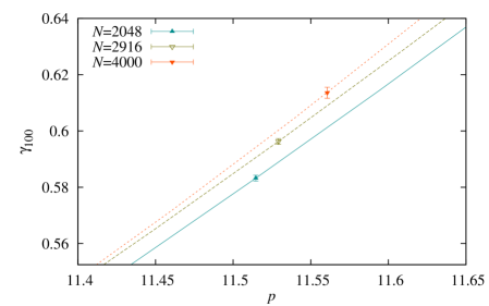
Figure 19: (Color online) Interfacial free-energy for the $(100)$ lattice crystalline direction $\gamma_{100}$ as a function of pressure, for a system of $N$ hard-spheres, for $N=2048,2916$ $N=4000$. We estimated $\gamma_{100}$ from Eq. 86

6 Conclusions

In this work, we have explained Tethered Monte Carlo fernandez:09 , a systematic and very general methodology to overcome free-energy barriers in Monte Carlo simulations without a random-walk in the reaction-coordinate space. An admittedly weak point is that a deep physical insight is needed in order to identify a suitable reaction coordinate. Nevertheless, it is worth mentioning that this problem may be bypassed using real replicas cammarotta:10 .

The power of the method is illustrated in two famous problems of modern theoretical physics, the diluted antiferromagnet in an external field (DAFF), the physical realization of the random field Ising model, and the crystallization of hard spheres. In both cases, the tethered approach allows to go beyond the state of the art.

Let us stress that Tethered Monte Carlo is not limited to reproducing canonical mean values, but it is also suitable to address different physical questions that one would never ask in a canonical setting due to overwhelming technical difficulties. Our study of the pseudo phase coexistence in the DAFF, see Sect. 4.7 is one example. Furthermore, for disordered systems, tethered Monte Carlo provides a redefinition of the quenched disorder, less vulnerable to (trivial) violations of self-averaging fernandez:08 ; fernandez:11b .

We remark as well that, from the algorithmic point of view, we have been rather unsophisticated. We used local Metropolis moves that (in the case of the DAFF) were complemented with parallel tempering. Clearly enough there is much room for improvements on this side (see e.g. martin-mayor:09 for an implementation of a cluster algorithm).

We also note that, in our implementation, both for the DAFF and for hard spheres there is a maximum system size beyond which one cannot equilibrate within reasonable computer time. Clearly enough new free-energy barriers appear, which are not adequately described by the chosen reaction coordinates. These could be treated by extending the number (or the type) of tethered quantities.

Appendix A Assessing thermalization in Monte Carlo simulations

This appendix is intended as a brief and handy reference on thermalization in Monte Carlo simulations, providing some definitions that are used throughout the paper (see sokal:97 for a detailed discussion). Most of the definitions are standard, but subsection A.1 describes a powerful thermalization criterion that may be new even for the Monte Carlo specialist.

As a general rule, the thermalization of a Monte Carlo simulation should be assessed through the temporal autocorrelation functions sokal:97 . If $O(t)$ is the measured value of the observable $O$ at time $t$ during the simulation, then

$$C_{O}(t,\hat{m})=\bigl{\langle}[O(0)-\langle O\rangle_{\hat{m}}][O(t)-\langle O\rangle_{\hat{m}}]\bigr{\rangle}_{\hat{m}},,\qquad\rho_{O}(t,\hat{m})=\frac{C_{O}(t,\hat{m})}{C_{O}(0,\hat{m})}\ .$$ (87)

From this function we obtain the integrated and exponential autocorrelation times

$$\tau_{\text{int},O}(\hat{m}) =\frac{1}{2}+\sum_{t=1}^{\infty}\rho_{O}(t,\hat{m}),$$ (88)

$$\tau_{\text{exp},O}(\hat{m}) =\lim_{t\to\infty}\sup\frac{t}{-\log|\rho_{O}(t,\hat{m})|},$$ (89)

$$\tau_{\text{exp}}(\hat{m}) =\sup_{O}\tau_{\text{exp},O}(\hat{m}).$$ (90)

In general, the autocorrelation function can be expressed as a sum of exponentials

$$\rho_{O}(t,\hat{m})=\sum_{i}A_{i}\mathrm{e}^{-t/\tau_{i}}.$$ (91)

The exponential time, then, is the largest of the $\tau_{i}$ and characterizes the time needed to equilibrate a certain observable (or the whole system). The integrated time indicates the minimum time difference so that two measurements of some observable $O$ can be considered independent (i.e., uncorrelated). Notice that if the decomposition (91) contains a single exponential, $\tau_{\text{exp},O}=\tau_{\text{int},O}$, This is a useful observation because the exponential time is harder to measure accurately than the integrated one.

A.1 Thermalization in parallel tempering simulations

The computation of the $\tau_{O}$ requires a much longer simulation time than what is needed to thermalize the system. This is not a problem for ordered systems, since extending the simulation reduces the statistical errors. In disordered systems, however, the errors are dominated by sample-to-sample fluctuations, so an efficient CPU time allocation should run each sample for a time long enough to thermalize it, but no longer. Therefore, the computation of autocorrelation times in these cases has traditionally been abandoned as impractical and thermalization is typically assessed by less rigorous methods such as the time evolution of disorder-averaged observables.

The use of parallel tempering, however, provides a way to compute the autocorrelation times in relatively short simulations. The key is analyzing quantitatively the temperature random walk of each participating configuration fernandez:09b . Reference janus:10 includes a detailed discussion of this method, here we shall only give a brief sketch of it.

Let us consider a parallel tempering simulation with $N_{T}$ participating replicas of the system. We define $f_{i}(t)$ as the function indicating the temperature index of replica $i$ at time $t$. By ‘temperature index’ we mean the temperature mapped onto $\{1,2,\ldots,N_{T}\}$, where $1$ corresponds to the lowest temperature and $N_{T}$ to the highest. We can now compute the autocorrelation function (87) of each $f_{i}$ (notice that $\langle f_{i}\rangle=(N_{T}+1)/2$). The $N_{T}$ correlation functions thus obtained can be averaged, so they collectively have the precision of a much longer simulation.

References

- (1) Landau, D.P., Binder, K.: A Guide to Monte Carlo Simulations in Statistical Physics. Cambridge University Press, Cambridge, second edn. (2005)
- (2) Lee, J., Kosterlitz, J.M.: Phys. Rev. Lett. 65, 137 (1990)
- (3) ten Wolde, P., Ruiz-Montero, M.J., Frenkel, D.: Phys. Rev. Lett. 75, 2714 (1995)
- (4) Zaccarelli, E., Valeriani, C., Sanz, E., Poon, W.C.K., Cates, M.E., Pusey, P.N.: Phys. Rev. Lett. 103, 135704 (2009)
- (5) Nattermann, T.: In: Spin glasses and random fields (ed. A.P. Young). World Scientific, Singapore (1998)
- (6) Ogielski, A.: Phys. Rev. Lett. 57, 1251 (1986)
- (7) Mézard, M., Parisi, G., Virasoro, M.: Spin-Glass Theory and Beyond. World Scientific, Singapore (1987)
- (8) Marinari, E., Parisi, G., Ricci-Tersenghi, F., Ruiz-Lorenzo, J.J., Zuliani, F.: J. Stat. Phys. 98, 973 (2000)
- (9) Hukushima, K., Nemoto, K.: J. Phys. Soc. Japan 65, 1604 (1996)
- (10) Marinari, E.: In: Advances in Computer Simulation (eds. J. Kerstész, I. Kondor). Springer-Berlag (1998)
- (11) Ogielski, A.: Phys. Rev. B 32, 7384 (1985)
- (12) Cruz, A., Pech, J., Tarancon, A., Tellez, P., Ullod, C.L., Ungil, C.: Comp. Phys. Comm 133, 165 (2001)
- (13) Ballesteros, H.G., Cruz, A., Fernandez, L.A., Martin-Mayor, V., Pech, J., Ruiz-Lorenzo, J.J., Tarancon, A., Tellez, P., Ullod, C.L., Ungil, C.: Phys. Rev. B 62, 14237 (2000)
- (14) Jimenez, S., Martin-Mayor, V., Perez-Gaviro, S.: Phys. Rev. B 72, 054417 (2005)
- (15) Belletti, F., Mantovani, F., Poli, G., Schifano, S.F., Tripiccione, R., Campos, I., Cruz, A., Navarro, D., Perez-Gaviro, S., Sciretti, D., Tarancon, A., Velascco, J.L., Tellez, P., Fernandez, L.A., Martin-Mayor, V., Muñoz Sudupe, A., Jimenez, S., Maiorano, A., Marinari, E., Ruiz-Lorenzo, J.J. (Janus Collaboration): Computing in Science and Engineering 8, 41 (2006)
- (16) Belletti, F., Cotallo, M., Cruz, A., Fernandez, L.A., Gordillo, A., Maiorano, A., Mantovani, F., Marinari, E., Martin-Mayor, V., Monforte, J., Muñoz Sudupe, A., Navarro, D., Perez-Gaviro, S., Ruiz-Lorenzo, J.J., Schifano, S.F., Sciretti, D., Tarancon, A., Tripiccione, R., Velasco, J. (Janus Collaboration): Comp. Phys. Comm. 178, 208 (2008)
- (17) Belletti, F., Cotallo, M., Cruz, A., Fernandez, L.A., Gordillo-Guerrero, A., Guidetti, M., Maiorano, A., Mantovani, F., Marinari, E., Martin-Mayor, V., Muñoz Sudupe, A., Navarro, D., Parisi, G., Perez-Gaviro, S., Ruiz-Lorenzo, J.J., Schifano, S.F., Sciretti, D., Tarancon, A., Tripiccione, R., Velasco, J., Yllanes, D. (Janus Collaboration): Phys. Rev. Lett. 101, 157201 (2008)
- (18) Belletti, F., Guidetti, M., Maiorano, A., Mantovani, F. Schifano, S.F., Tripiccione, R., Cotallo, M., Perez-Gaviro, S., Sciretti, D., Velasco, J.L., Cruz, A., Navarro, D., Tarancon, A., Fernandez, L.A., Martin-Mayor, V., Muñoz-Sudupe, A., Yllanes, D., Gordillo-Guerrero, A., Ruiz-Lorenzo, J.J., Marinari, E., Parisi, G., Rossi, M., Zanier, G. (Janus Collaboration): Computing in Science and Engineering 11, 48 (2009)
- (19) Belletti, F., Cruz, A., Fernandez, L.A., Gordillo-Guerrero, A., Guidetti, M., Maiorano, A., Mantovani, F., Marinari, E., Martin-Mayor, V., Monforte, J., Muñoz Sudupe, A., Navarro, D., Parisi, G., Perez-Gaviro, S., Ruiz-Lorenzo, J.J., Schifano, S.F., Sciretti, D., Tarancon, A., Tripiccione, R., Yllanes, D. (Janus Collaboration): J. Stat. Phys. 135, 1121 (2009)
- (20) Álvarez Baños, R., Cruz, A., Fernandez, L.A., Gil-Narvion, J.M., Gordillo-Guerrero, A., Guidetti, M., Maiorano, A., Mantovani, F., Marinari, E., Martin-Mayor, V., Monforte-Garcia, J., Muñoz Sudupe, A., Navarro, D., Parisi, G., Perez-Gaviro, S., Ruiz-Lorenzo, J., Schifano, S.F., Seoane, B., Tarancon, A., Tripiccione, R., Yllanes, D. (Janus Collaboration): J. Stat. Mech. P06026 (2010)
- (21) Álvarez Baños, R., Cruz, A., Fernandez, L.A., Gil-Narvion, J.M., Gordillo-Guerrero, A., Guidetti, M., Maiorano, A., Mantovani, F., Marinari, E., Martin-Mayor, V., Monforte-Garcia, J., Muñoz Sudupe, A., Navarro, D., Parisi, G., Perez-Gaviro, S., Ruiz-Lorenzo, J., Schifano, S.F., Seoane, B., Tarancon, A., Tripiccione, R., Yllanes, D. (Janus Collaboration): Phys. Rev. Lett. 105, 177202 (2010)
- (22) Berg, B.A., Neuhaus, T.: Phys. Rev. Lett. 68, 9 (1992)
- (23) Wang, F., Landau, D.P.: Phys. Rev. Lett. 86, 2050 (2001)
- (24) Biskup, M., Chayes, L., Kotecký, R.: Europhys. Lett. 60, 21 (2002)
- (25) Binder, K.: Physica A (Amsterdam) 319, 99 (2003)
- (26) MacDowell, L.G., Virnau, P., Müller, M., Binder, K.: J. Chem. Phys. 120, 5293 (2004)
- (27) MacDowell, L.G., Shen, V., Errington, J.R.: J. Chem. Phys. 125, 034705 (2006)
- (28) Nußbaumer, A., Bittner, E., Neuhaus, T., Janke, W.: Europhys. Lett. 75, 716 (2006)
- (29) Neuhaus, T., Hager, J.: J. of Stat. Phys. 113, 47 (2003)
- (30) Lustig, R.: J. Chem. Phys. 109, 8816 (1998)
- (31) Martin-Mayor, V.: Phys. Rev. Lett. 98, 137207 (2007)
- (32) Janke, W.: Nucl. Phys. 63, 631 (1998)
- (33) Chopra, M., Müller, M., de Pablo, J.J.: J. Chem. Phys 124, 134102 (2006)
- (34) Steinhardt, P.J., Nelson, D.R., Ronchetti, M.: Phys. Rev. B 28, 784 (1983)
- (35) Torrie, G.M., Valleau, J.P.: J. Comp. Physics. 23, 187 (1977)
- (36) Fernandez, L.A., Martin-Mayor, V., Yllanes, D.: Nucl. Phys. B 807, 424–454 (2009)
- (37) Martin-Mayor, V., Yllanes, D.: Phys. Rev. E 80, 015701(R) (2009)
- (38) Fernández, L., Martin-Mayor, V., Seoane, B., Verrocchio, P.: (2011). arXiv:1103.2599
- (39) Fernandez, L.A., Martin-Mayor, V., Yllanes, D.: (2011). arXiv:1106.1555
- (40) Yllanes, D.: Ph.D. Thesis. UCM (in preparation)
- (41) Seoane, B.: Ph.D. Thesis. UCM (in preparation)
- (42) Cammarota, C., Cavagna, A., Giardina, I., Gradenigo, G., Grigera, T.S., Parisi, G., Verrocchio, P.: Phys. Rev. Lett. 105, 055703 (2010)
- (43) Metropolis, N., Rosenbluth, A.W., Rosenbluth, N.M., Teller, A.H., Teller, E.: J. Chem. Phys. 21, 1087 (1953)
- (44) Amit, D.J., Martin-Mayor, V.: Field Theory, the Renormalization Group and Critical Phenomena. World Scientific, Singapore, third edn. (2005)
- (45) Sokal, A.D.: In: Functional Integration: Basics and Applications (1996 Cargèse School) (eds. C. DeWitt-Morette, P. Cartier, A. Folacci). Plenum, N.Y. (1997)
- (46) Kasteleyn, P.W., Fortuin, C.M.: J. Phys. Soc. Jpn Suppl. 26s, 11 (1969)
- (47) Fortuin, C.M., Kasteleyn, P.W.: Physica (Utrecht) 57, 536 (1972)
- (48) Swendsen, R.H., Wang, J.S.: Phys. Rev. Lett. 58, 86 (1987)
- (49) Wolff, U.: Phys. Rev. Lett. 62, 361 (1989)
- (50) Edwards, R.G., Sokal, A.D.: Phys. Rev. D 38, 2009 (1988)
- (51) Belanger, D.P.: In: Spin Glasses and Random Fields (ed. A.P. Young). World Scientific, Singapore (1997)
- (52) Fishman, S., Aharony, A.: J. Phys. C 12, L729 (1979)
- (53) Cardy, J.: Phys. Rev. B 29, 505 (1984)
- (54) de Dominicis, C., Giardina, I.: Random Fields and Spin Glasses. Cambridge University Press, Cambridge, England (2006)
- (55) Vink, R.L.C., Fischer, T., Binder, K.: Phys. Rev. E 82, 051134 (2010)
- (56) Hartmann, A.K., Young, A.P.: Phys. Rev. B 64, 214419 (2001)
- (57) Slanic, Z., Belanger, D.P., Fernandez-Baca, J.A.: Phys. Rev. Lett. 82, 426 (1999)
- (58) Ye, F., Zhou, L., Larochelle, S., Lu, L., Belanger, D.P., Greven, M., Lederman, D.: Phys. Rev. Lett. 89, 157202 (2002)
- (59) Sourlas, N.: Comp. Phys. Comm. 121, 183 (1999)
- (60) Maiorano, A., Martin-Mayor, V., Ruiz-Lorenzo, J.J., Tarancón, A.: Phys. Rev. B 76, 064435 (2007)
- (61) Belanger, D.P., King, A.R., Jaccarino, V., Cardy, J.L.: Phys. Rev. B 28, 2522 (1983)
- (62) Belanger, D.P., Slanic, Z.: J. Magn. and Magn. Mat. 186, 65 (1998)
- (63) Parisi, G., Sourlas, N.: Phys. Rev. Lett. 89, 257204 (2002)
- (64) Fischer, T., Vink, R.L.C.: J. Phys. Condens. Matt. 23, 234117 (2011).
- (65) Stauffer, D., Aharony, A.: In: Introduction to the Percolation Theory. Taylor and Francis, London (1984)
- (66) Aharony, A., Harris, A.B.: Phys. Rev. Lett 77, 3700 (1996)
- (67) Wiseman, S., Domany, E.: Phys. Rev. Lett. 81, 22 (1998)
- (68) Malakis, A., Fytas, N.G.: Phys. Rev. E 73, 016109 (2006)
- (69) Fernandez, L.A., Gordillo-Guerrero, A., Martin-Mayor, V., Ruiz-Lorenzo, J.J.: Phys. Rev. Lett. 100, 057201 (2008)
- (70) Fernandez, L.A., Martin-Mayor, V.: Phys. Rev. E 79, 051109 (2009)
- (71) Fernandez, L.A., Maiorano, A., Marinari, E., Martin-Mayor, V., Navarro, D., Sciretti, D., Tarancon, A., Velasco, J.L.: Phys. Rev. B 77, 104432 (2007)
- (72) Alder, B.J., Wainwright, T.E.: J. Chem. Phys. 27, 1208 (1957)
- (73) Wood, W.W., Jacobson, J.D.: J. Chem. Phys. 27, 1207 (1957)
- (74) Pusey, P.N., van Megen: Nature 320, 340 (1986)
- (75) Pusey, P.N., van Megen, W., Bartlett, P., Ackerson, B.J., Rarity, J.G., Underwood, S.M.: Phys. Rev. Lett. 63, 2753 (1989)
- (76) Vega, C., Sanz, E., Abascal, J.L.F., Noya, E.G.: J. Phys.: Condens. Matter 20, 153101 (2008)
- (77) Wilding, N.B., Bruce, A.D.: Phys. Rev. Lett. 85, 5138 (2000)
- (78) Errington, J.R.: J. Chem. Phys. 120, 3130 (2000)
- (79) Hoover, W.G., Ree, F.H.: J. Chem. Phys 49, 3609 (1968)
- (80) Frenkel, D., Ladd, A.K.C.: J. Chem. Phys. 81, 3188 (1984)
- (81) Polson, J.M., Trizac, E., Pronk, S., Frenkel, D.: J. Chem. Phys. 112, 5339 (2000)
- (82) Vega, C., Noya, E.G.: J. Chem. Phys. 127, 154113 (2007)
- (83) Ladd, J.C., Woodcock, L.V.: J. Chem. Phys. 51, 155 (1977)
- (84) Noya, E.G., Vega, C., de Miguel, E.: J. Chem. Phys. 128, 154507 (2008)
- (85) Zykova-Timan, T., Horbach, J., Binder, K.: J. Chem. Phys 133, 014705 (2010)
- (86) van Duijneveldt, J.S., Frenkel, D.: J. Chem. Phys 96, 4655 (1992)
- (87) Angioletti-Uberti, S., Ceriotti, M., Lee, P.D., Finnis, M.W.: Phys. Rev. B 81, 125416 (2010)
- (88) Falcioni, M., Marinari, E., Paciello, M.L., Parisi, G., Taglienti, B.: Phys. Lett. 108, 331 (1982)
- (89) Ferrenberg, A.M., Swendsen, R.H.: Phys. Rev. Lett. 61, 2635 (1988)
- (90) Davidchack, R.L., Laird, B.B.: Phys. Rev. Lett. 85, 4751 (2000)
- (91) Mu, Y., Houk, A., Song, X.: J. Phys. Chem. B 109, 6500 (2005)
- (92) Davidchack, R.L.: J. Chem. Phys. 133, 234701 (2010)
- (93) Fernandez, L.A., Martin-Mayor, V., Perez-Gaviro, S., Tarancon, A., Young, A.P.: Phys. Rev. B 80, 024422 (2009)