GravitoMagnetic Force in Modified Newtonian Dynamics

Abstract

We introduce the Gauge Vector-Tensor (GVT) theory by extending the AQUAL’s approach to the GravitoElectroMagnetism (GEM) approximation of gravity. GVT is a generally covariant theory of gravity composed of a pseudo Riemannian metric and two $U(1)$ gauge connections that reproduces MOND in the limit of very weak gravitational fields while remains consistent with the Einstein-Hilbert gravity in the limit of strong and Newtonian gravitational fields. GVT also provides a simple framework to study the GEM approximation to gravity. We illustrate that the gravitomagnetic force at the edge of a galaxy can be in accord with either GVT or $\Lambda$CDM but not both. We also study the physics of the GVT theory around the gravitational saddle point of the Sun and Jupiter system. We notice that the conclusive refusal of the GVT theory demands measuring either both of the gravitoelectric and gravitomagnetic fields inside the Sun-Jupiter MOND window, or the gravitoelectric field inside two different solar GVT MOND windows. The GVT theory, however, will be favored by observing an anomaly in the gravitoelectric field inside a single MOND window.

1 Introduction

Either $95\%$ of the observed universe is made of things that have not yet been observed in the Solar system, or the law of dynamics or gravity should be modified in very low accelerations or very weak gravitational fields. The $\Lambda$-CDM model of cosmology buys the first approach. Its challenges [1, 2], however, signal that "the physics of the dark sector is, at the very least, much richer and complex than currently assumed, and that our understanding of gravity and dynamics might also be at play" [3]. The second approach is the modified theories of gravity. The modified theories of gravity can be classified into the following two categories:

1. Phenomenological search for the dynamics of the metric.

2. Introducing new degrees of freedom for gravity in addition to the metric.

The first class assumes that gravity is described by a pseudo Riemannian metric and the action of gravity is given by

$$S=\int\sqrt{-\det g}\big{(}{\cal L}_{g}[g_{\mu\nu},R_{\mu\nu\lambda\eta},\nabla_{\mu}]+{\cal L}_{m}[\Psi]\big{)}\,,$$ (1.1)

where $R_{\mu\nu\lambda\eta}$ is the Riemann tensor constructed out of the metric $g_{\mu\nu}$, ${\cal L}_{m}[\Psi]$ is the matter’s action not necessarily minimally coupled to the metric, and ${\cal L}_{g}$ is the gravity’s action. The Einstien-Hilbert theory assumes ${\cal L}_{g}=R$ where $R$ is the Ricci scalar. The purchasers of this class choose to reject the Einstein-Hilbert assumption and search for families of ${\cal L}_{g}$ reproducing the dynamics of nature in large scales. Considering the infinite number of possibilities in choosing $\cal L$ and the finite set of the cosmological data, this purchase will work [4]. It would not necessarily be in accord with the principle of the Occam’s razor. It also will lead to a set of nonlinear partial differential equations of degrees larger than two, a set of equations which most of rational humans would despise. These are, however, the prices to pay.

The second class of the modified theories of gravity introduces new degrees of freedom in addition to the metric to describe gravity. The most known example of this class is the TeVeS theory [5]. TeVeS introduces a pseudo Riemannian metric, a scalar and a vector field in order to phenomenologically describe the physics in very weak gravitational fields (the MOND regime) . The TeVeS theory defines new nonlinearity in order to solve the physics of the MOND regime. The introduced nonlinearity, however, is not local to the MOND regime of the theory. It continues to the very strong gravity regime of theory. The physics of very strong gravitational systems, therefore, strongly constrain the TeVeS theory. This signals that the introduced nonlinearity of the TeVeS is not appropriate to describe the physics of the MOND regime. One should define a nonlinearity capable of producing the physics of the MOND system such that the nonlinearity does not propagate all the way down to the Newtonian and strong regime of the theory. In order to perform such a definition, we go back to the very root of the TeVeS theory: the AQUAL theory. We show how to apply the AQUAL procedure upon the GravitoElectroMagnetism approximation of gravity. This introduces a non-covariant version for GEM in MOND regime whose generally covariant version demands introducing gauge vector fields rather than a scalar field. We, thus, introduce two $U(1)$ gauge vectors in addition to the metric and present a generally covariant theory for GEM in the MOND regime. This theory, which we call the Gauge Vector Tensor theory, reproduces MOND in the limit of very weak gravitational fields while remains consistent with the Einstein-Hilbert gravity in the limit of strong and Newtonian gravitational fields. In contrary to the TeVeS theory, the GVT theory is in total agreement with the physics of the strong gravity. Its equations of motion are also much simpler than those of the TeVeS theory.

The paper is organized as follows: Sections 2 and 3 review the GravitoElectroMagnetism (GEM) to gravity. Section 4 reviews the algorithm that leads to the AQUAL theory as a realization of the MOND paradigm. Section 5 applies the AQUAL’s algorithm to GEM. Section 6 introduces one gauge field and presents a covariant realization of the GEM to MOND. It also discusses the phenomenological constraints on the theory. Section 7 introduces an additional gauge field in order to make the theory fully consistent with the predictions of the Einstein-Hilbert theory for the strong and Newtonian gravitational field. Section 8 studies various regimes of the GVT theory. The GVT theory possesses the Newtonian and strong regime of gravity, the MOND regime and the post-MONDian regime. Section 9 calculates the gravitomagnetic field of a spinning galaxy in the $\Lambda$CDM theory and the GVT theory. It shows that the gravitomagnetic field of a galaxy can be in accord with only one of them. Section 10 studies the physics of the GVT theory around the gravitational saddle point of the Sun and Jupiter system. It notices that the conclusive refusal of the GVT theory demands measuring either both of the gravitoelectric and gravitomagnetic fields inside the Sun-Jupiter MOND window, or the gravitoelectric field inside two different solar GVT MOND windows. It concludes that the GVT theory, however, can be favored by observing an anomaly in the gravitoelectric field inside a single MOND window. Section 11 provides the conclusion and outlook.

2 Response of the test probes to the gravitomagnetic field

Classical gravity is governed by a single scalar field, the gravitational potential. The Newtonian gravitational potential satisfies:

$$\nabla^{2}\Phi=4\pi G\rho,$$ (2.1)

where $\rho$ is the density of matter. Albert Einstein attempting to uplift gravity to a relativistic regime, first replaced the space-time metric of Minkowski by

$$ds^{2}\,=\,-c(\Phi)^{2}dt^{2}+dx^{2}+dy^{2}+dz^{2},$$ (2.2)

later with the Gromann’s help, he introduced the Riemannian metric,

$$ds^{2}\,=\,g_{\mu\nu}dx^{\mu}dx^{\nu},$$ (2.3)

as the relativistic gravity [6]. The relativistic theory of gravity has a symmetric rank-two tensor: the metric. The metric has 10 components in four dimensions, 9 more than the degrees of the classical gravity. To perceive the physical meaning of the degrees of the freedom of the relativistic theory, let the trajectory of a slow moving particle be considered in a static deviation from the Minkiowki metric. In so doing, the metric reads

$$ds^{2} = \eta_{\mu\nu}dx^{\mu}dx^{\nu}+h_{\mu\nu}dx^{\mu}dx^{\nu}\,,$$ (2.4)

$$h_{\mu\nu} = h_{\mu\nu}(x^{i})\,,$$ (2.5)

$$h_{\mu\nu} \ll 1\,.$$ (2.6)

Only for a relativistic mass distribution like a geon [7] the off-diagonal components of $h_{ij}$ are comparable to its other components. The contribution of the $h_{ij}$ are also suppressed for the orbits of slow moving particles. We are considering the geometry around a non-relativistic mass distribution. We also study the orbits of massive slow moving particles. In these circumstances the orbit of the particles can be derived from

$$S=-\frac{m}{2}\int d\tau g_{\mu\nu}\dot{x}^{\mu}\dot{x}^{\nu}\approx-\frac{m}{2}\int d\tau\left(c^{2}(-1+2A_{0})\dot{t}^{2}+(\dot{x}^{i})^{2}+2cA_{i}\dot{t}\dot{x}^{i}\right)\,,$$ (2.7)

wherein $\sum_{i\neq j}h_{ij}\dot{x}^{i}\dot{x}^{j}$ has been ignored, and $\tau$ is an affine parameter and

$$c^{2}A_{0} \equiv \frac{1}{2}h_{00}\,,$$ (2.8a)

$$cA_{i} \equiv h_{i0}\,,$$ (2.8b)

and

$${}^{.}=\frac{\partial}{\partial\tau}\,.$$ (2.9)

The Euler-Lagrange equation for $t$ derived from (2.7) reads

$$c^{2}\dot{t}(-1+2A_{0})+2cA_{i}\dot{x}^{i}\,=\,cte\,,$$ (2.10)

where $\dot{t}(-1+2A_{0})$ stands for the gravitational redshift while $2A_{i}\dot{x}^{i}$ represents a relativistic term. Eq. (2.10) can be solved for $t$ in term of $\tau$:

$$t=\tau+O(A)\,,$$ (2.11)

wherein appropriate unite of time is chosen. The Euler-Lagrange equation for $x^{i}$ derived from (2.7) then leads to

$$\frac{d^{2}x^{i}}{d\tau^{2}}=c^{2}\partial^{i}A_{0}+c\delta^{ij}(\partial_{k}A_{j}-\partial_{j}A_{k})\frac{dx^{k}}{d\tau}\,.$$ (2.12)

Utilizing (2.11) then results

$$\frac{d^{2}x^{i}}{dt^{2}}=c^{2}\partial^{i}A_{0}+c\delta^{ij}(\partial_{k}A_{j}-\partial_{j}A_{k})\frac{dx^{k}}{dt}+O(A^{2})\,.$$ (2.13)

Now let it be redefined

$$A_{0} \to \frac{1}{c^{2}}A_{0}=\Phi\,,$$ (2.14)

$$A_{i} \to \frac{1}{c^{2}}A_{i}\,,$$ (2.15)

using which the equation (2.13) can be rewritten as follows

$$\ddot{x}=-\nabla\Phi+\frac{v}{c}\times(\nabla\times A)\,.$$ (2.16)

This allows interpreting $\nabla\times A$ as a gravitomagnetic field. $\nabla\times A$ causes precessions of the orbits of a test particle. This precession is referred to as the Lense-Thirring precession [9]. Ref. [10] provides a decent recent review on Lense-Thirring precession for planets and satellites in the Solar system. The similarity between the gravitomagnetic field and magnetic field beside the spin precession formula in electrodynamics ($\dot{S}=\mu\times B,\mu=\frac{e}{2m}S$) dictates that the spin of a gyroscope precesses by [11]

$$\Omega_{LT}=-\frac{1}{2}\nabla\times A\,.$$ (2.17)

This precession is called the Pugh-Schiff frame-dragging precession [12, 13]. The Pugh-Schiff frame-dragging precession due to the rotation of the earth recently has been measured by the gravity probe B with the precision of 19% [14]. GINGER, aiming to improve the sensitivity of the ring resonators, plans to measure the gravitomagnetic effect with a precision at least one order better than that of the gravity probe B [15]. Also LAGEOS and LAGEOS 2, and with a number of GRACE (Gravity Recovery and Climate Experiment) have confirmed the prediction of Einstein General Relativity for the Earth’s gravitomagnetic field with with an accuracy of approximately 10% [16]. Ref. [17] shows that the gravitomagnetic field of the Earth is in agreement with the Einstein theory’s prediction with approximately 0.1% accuracy via lunar laser ranging (LLR).

3 GravitoElectroMagnetism approximation

In the linearized Einstein-Hilbert gravity, the Einstein field equations written in the harmonic gauge simplifies to

$$\Box\bar{h}_{\mu\nu} = -16\pi GT_{\mu\nu}^{(0)}\,,$$ (3.1)

$$\partial_{\mu}\bar{h}^{\mu\nu} = 0\,,$$ (3.2)

where $\bar{h}_{ij}$ is the trace reversed perturbation

$$\bar{h}_{\mu\nu}\,\equiv\,h_{\mu\nu}-\frac{1}{2}\eta_{\mu\nu}h^{\alpha}_{~{}\alpha}\,.$$ (3.3)

We notice that the linearized equations can be derived from

$$S=\int d^{4}x(-\frac{1}{2}\partial_{\alpha}\bar{h}_{\mu\nu}\partial^{\alpha}\bar{h}^{\mu\nu}+16\pi G\bar{h}_{\mu\nu}T^{\mu\nu}+\lambda_{\nu}\partial_{\mu}\bar{h}^{\mu\nu})\,,$$ (3.4)

where $\lambda_{\nu}$ is a local Lagrange multiplier enforcing (3.2), and $T^{\mu\nu}$ represents the linear energy-momentum tensor. Note that the effective action is invariant under the residual symmetry of the harmonic gauge. It is invariant under

$$h_{\mu\nu} \to h_{\mu\nu}+\partial_{\mu}\xi_{\nu}+\partial_{\nu}\xi_{\mu}\,,$$ (3.5a)

$$\Box\xi_{\mu} = 0\,.$$ (3.5b)

We do not fix the residual symmetry. We consider it as the symmetry of the action. We decompose $\bar{h}_{\mu\nu}$ to

$$\bar{h}_{\mu\nu}dx^{\mu}dx^{\nu}\equiv\bar{A}_{0}dt^{2}+\bar{A}_{i}dx^{i}dt+\bar{h}_{ij}dx^{i}dx^{j}\,.$$ (3.6)

Inserting (3.6) into (3.4) yields:

$$S=\int d^{4}x(\frac{1}{2}\bar{A}_{0}\Box\bar{A}_{0}+\bar{A}_{i}\Box\bar{A}_{i}+\frac{1}{2}\bar{h}_{ij}\Box\bar{h}^{ij}+16\pi G\rho\bar{A}_{0}+32\pi G\bar{A}_{i}J^{i}+16\pi G\bar{h}_{ij}T^{ij})\,,$$ (3.7)

and the constraints read

$$\partial^{\mu}\bar{A}_{\mu} = 0\,,$$ (3.8)

$$\partial_{0}\bar{A}_{i}-\partial_{j}\bar{h}^{j}_{~{}i} = 0\,.$$ (3.9)

The action of (3.7) at the level of the equations of motion is equivalent to

$$S=\int d^{4}x(-\frac{1}{2}\bar{A}_{0}\Box\bar{A}_{0}+\frac{1}{2}\bar{A}_{i}\Box\bar{A}_{i}+\frac{1}{2}\bar{h}_{ij}\Box\bar{h}^{ij}+16\pi G\bar{A}_{i}J^{i}-16\pi G\rho\bar{A}_{0}+16\pi G\bar{h}_{ij}T^{ij})\,.$$ (3.10)

Now let it be defined:

$$\bar{A}_{\mu} \equiv (\bar{A}_{0},\bar{A}_{i})\,,$$ (3.11)

$$J_{\mu} \equiv (\rho,J_{i})=T_{0\mu}\,.$$ (3.12)

Then (3.10) simplifies to

$$S=\int d^{4}x(\frac{1}{2}\bar{A}_{\mu}\Box\bar{A}^{\mu}+\frac{1}{2}\bar{h}_{ij}\Box\bar{h}^{ij}+16\pi G\bar{A}_{\mu}J^{\mu}+16\pi G\bar{h}_{ij}T^{ij})\,,$$ (3.13)

Eq. (3.8) yields:

$$\frac{1}{2}\int d^{4}x\bar{A}_{\mu}\Box\bar{A}^{\mu}=\frac{1}{2}\int d^{4}x\bar{A}_{\mu}(\Box\eta^{\mu\nu}-\partial^{\mu}\partial^{\nu})\bar{A}_{\nu}=-\int d^{4}x\frac{1}{4}\bar{F}_{\mu\nu}\bar{F}^{\mu\nu}\,,$$ (3.14)

where

$$\bar{F}_{\mu\nu}\equiv\partial_{\mu}\bar{A}_{\nu}-\partial_{\nu}\bar{A}_{\mu}\,\,.$$ (3.15)

Utilizing (3.14) re-expresses (3.13) to:

$$S = \int d^{4}x({\cal L}_{g}+{\cal L}_{S}+{\cal L}_{\lambda})\,,$$ (3.16a)

$${\cal L}_{g} \equiv -\frac{1}{4}\bar{F}_{\mu\nu}\bar{F}^{\mu\nu}-\frac{1}{2}\partial_{\alpha}\bar{h}_{ij}\partial^{\alpha}\bar{h}^{ij}\,,$$ (3.16b)

$${\cal L}_{s} \equiv 16\pi G\bar{A}_{\mu}J^{\mu}+16\pi G\bar{h}_{ij}T^{ij}\,,$$ (3.16c)

$${\cal L}_{\lambda} \equiv \lambda_{0}\partial^{\mu}\bar{A}_{\mu}+\lambda^{i}(\partial_{0}\bar{A}_{i}-\partial_{j}\bar{h}_{i}^{~{}j})\,,$$ (3.16d)

The first term of ${\cal L}_{g}$ in (3.16b) is the GravitoElectoMagnetic (GEM) approximation to gravity. ${\cal L}_{s}$ in (3.16c) describes how the fields couple to the sources (Energy momentum tensor). ${\cal L}_{\lambda}$ in (3.16d) is the gauge fixing Lagrangian. In comparison to the electrodynamics, the equations of motion for $\lambda$ impose two extra conditions of (3.8) and (3.9) on $\bar{A}_{\mu}$. Eq. (3.8) states that the GEM should be solved in the Lorentz gauge. Eq. (3.9) implies that GEM has wave solutions only if $\bar{h}_{ij}$ field possesses a wave solution. The wave solution is due to the dynamics of the $\bar{h}_{ij}$ field. This means that though the GEM is akin to the ordinary electrodynamics it lacks radiation.

Near and around the galaxies, $\bar{h}_{ij}$ is suppressed due to the non-relativistic velocity of the stars and gas inside the galaxy. At the leading order $\bar{h}_{ij}$ also does not affect the orbits of slow-moving massive particles. Slow moving particles see only the GEM part of the metric (2.7). Since we are interested in the orbits of slow moving massive particles around a galaxy we just consider only the GEM part of (3.16):

$$S = \int d^{4}x({\cal L}_{A}+16\pi G\bar{A}_{\mu}J^{\mu}+\lambda\partial^{\mu}\bar{A}_{\mu})\,,$$ (3.17a)

$${\cal L}_{A} = -\frac{1}{4}\bar{F}_{\mu\nu}\bar{F}^{\mu\nu}\,.$$ (3.17b)

Also note that time dependent $A_{\mu}$ , through the constraint equation (3.9), induces a time-dependent behavior for $h_{ij}$. The orbits of the stars at the leading approximation are blind to the change in $h_{ij}$. In the study of the orbits of the stars, therefore, the time dependent solutions of (3.17) are valid. The symmetry of the truncated Lagrangian (3.17b) is

$$\bar{A}_{\mu}\to\bar{A}_{\mu}+\partial_{\mu}\Lambda\,,$$ (3.18)

where $\Lambda$ is a general scalar field. Part of this symmetry is broken by the gauge fixing Lagrangian.

4 AQUAL as a Realization of MOND

The Newtonian approximation of the linearized GEM action (3.17) reads

$$\bar{A}_{\mu}(x,t) = (4\Phi(x),\vec{0})\,,$$ (4.1)

$$J_{\mu} = (\rho(x),\vec{0})\,,$$ (4.2)

Notice that $\bar{A}_{0}$ is equal to $4\Phi$ rather than $2\Phi$ because $\bar{A}_{\mu}$ comes from the trace reversed metric. For the reversed trace metric $\bar{h}_{00}=4\phi$ and $\bar{h}_{ij}=0$ give $h_{00}=2\phi$ and $h_{ii}=-2\phi$. Inserting the Newtonian approximation into (3.17) yields

$$S = -16\int d^{4}x\,(\frac{1}{2}|\nabla\phi|^{2}+4\pi G\rho\phi)\,.$$ (4.3)

Notice that (4.3) up to the overall factor of

$$16\int dt\,,$$ (4.4)

is equivalent to the Newtonian gravitational action:

$$S_{N}=-\int d^{3}x\left[|\nabla\Phi|^{2}+8\pi G\rho\Phi\right]\,.$$ (4.5)

In the Modified gravity realization of the MOND [18], one replaces the Newtonian classical field theory with a general field theory but retain the Newtonian dynamics ($F=ma$):

$$S_{MoG}=-\int d^{3}x\left[{\cal L}(\Phi,\nabla\Phi,\cdots)+8\pi G\rho\Phi\right]\,.$$ (4.6)

Keeping intact the Newtonian dynamics means that the orbits of slow moving particles are derived from (2.7). The AQUAL approach [19] assumes that the symmetries for the equations of motions derived from $S$ and $S_{MoG}$ are the same. The symmetries for $S$ are

$$\Phi\to\Phi+{\Lambda}\,,$$ (4.7)

where ${\Lambda}$ is constant. Imposing (4.7) on (4.6) requires $\cal L$ to be a functional of the derivative of the Newtonian potential:

$${\cal L}\,\equiv\,{\cal L}(\nabla\Phi,\nabla^{2}\Phi,\cdots)\,.$$ (4.8)

AQUAL also requires the equations to be second order. So the Lagrangian is simplified to

$${\cal L}\,\equiv\,{\cal L}(\nabla\Phi)\,.$$ (4.9)

We can construct only one scalar out of $\nabla\Phi$. So the Lagrangian reads

$${\cal L}\,\equiv\,{\cal F}(\frac{1}{a_{0}^{2}}\nabla\Phi.\nabla\Phi)\,,$$ (4.10)

and the AQUAL action follows

$$S_{AQUAL}=-\int d^{3}x\left[a_{0}^{2}{\cal F}(\nabla\Phi.\nabla\Phi/a_{0}^{2})+8\pi G\rho\Phi\right]\,.$$ (4.11)

The first variation of the AQUAL action with respect to $\Phi$ yields

$$\nabla^{\alpha}\left(\mu(\frac{|\nabla\Phi|}{a_{0}})~{}\nabla_{\alpha}\Phi\right)=4\pi G\rho,$$ (4.12)

where

$$\mu(x)\,\equiv\,\frac{d{\cal F}(y)}{dy}|_{y=x^{2}}={\cal F}^{\prime}(x^{2}).$$ (4.13)

The MOND terminology than requires [21]

$$\mu(x)\approx 1~{}:~{}\text{For}~{}x\gg 1\,,$$ (4.14a)

$$\mu(x)\approx x~{}:~{}\text{For}~{}x\leq 1\,,$$ (4.14b)

and

$$a_{0}=(1.0\pm 0.2)\times 10^{-10}\frac{m}{s^{2}}\,.$$ (4.15)

5 AQUAL Extension to GEM

Following the AQUAL model, we search for a non-linear generalization of (3.17) that leads to second-order differential equations. This generalization must coincide to the AQUAL model for a vanishing gravitomagnetic field. We are assuming that the physics of the MOND regime follows from $\bar{h}_{ij}=0$ and $\bar{h}_{00}\neq 0$. So $\det{g}$ in the harmonic gauge is independent of the mass distribution due to the equations of motion. This means that the space-time geometry around a spherical static mass distribution holds

$$g_{tt}(r)g_{rr}(r)=-1\,,$$ (5.1)

where $g_{tt}$ and $g_{rr}$ represent respectively the $tt$-component and $rr$-component of the metric in the standard spherical coordinates. We, therefore, implicitely consider models of modified gravity wherein the area-radius coordinate of their spherical-static solution is an affine parameter on the radial null geodesics [22].

The simplest non-linear Lagrangian density for $\bar{A}$ preserving (3.18) and leading to second-order differential equations is

$${\cal L}_{MOND} = -\tilde{\Large\cal L}\left(\frac{\bar{F}_{\mu\nu}\bar{F}^{\mu\nu}}{4a_{0}^{2}}\right)+16\pi G\bar{A}_{\mu}J^{\mu}\,,$$ (5.2)

which after taking the overall factor of 16 in (4.4) must coincide to (4.11) for $\bar{A}_{\mu}=(4\Phi,\vec{0})$. Imposing the consistency between (4.11) and (5.2), thus, gives:

$$\tilde{\Large\cal L}(8x)=16a_{0}^{2}{\cal F}(x)\to\tilde{\Large\cal L}(x)=16a_{0}^{2}{\cal F}(\frac{x}{8})\,.$$ (5.3)

The consistency between (5.2) and the AQUAL model (4.11) demands

$${\cal L}_{MOND} = -16a_{0}^{2}{\Large\cal F}\left(\frac{\bar{F}_{\mu\nu}\bar{F}^{\mu\nu}}{32a_{0}^{2}}\right)+16\pi G\bar{A}_{\mu}J^{\mu}\,.$$ (5.4)

And the equation of motion of $A_{\mu}$ reads

$$\nabla_{\nu}({\cal F}^{\prime}F^{\nu\mu})=16\pi GJ^{\mu}\,,$$ (5.5)

where

$${\cal F}^{\prime}=\frac{{\cal F}(x)}{dx}|_{x=-\frac{\bar{F}_{\mu\nu}\bar{F}^{\mu\nu}}{32a_{0}^{2}}}\,,$$ (5.6)

Note that this way of extending MOND to GEM is not generally covariant. Next sections provide a generally covariant realization of (5.4).

6 Toward the Gauge Vector-Tensor theory

The Bekenstein’s Tensor-Vector-Scaler theory [5] is a covariant realization of the AQUAL theory but does not reproduce (5.2). The observed gravitomagnetism, however, strongly constraints the free parameters of the TeVeS theory [24] . We would like to present a covariant generalization of (5.2). To this aim we assume that a gauge vector field $B_{\mu}$ and a pseudo Riemannian metric $g_{\mu\nu}$ govern the dynamics of the space-time geometry. We presume that the orbits of massive particles are derived from the variation of

$$S=-m\int d\tau\left(\sqrt{-\dot{x}^{\mu}\dot{x}^{\mu}g_{\mu\nu}(x)}+B_{\mu}\dot{x}^{\mu}\right)\,,$$ (6.1)

where $\tau$ is a parameter defined on the world-line. Eq. (6.1) is tantamount to saying that the physical length and time are defined in term of a Finsler/Randers geometry [27] of

$$S[\tau] = -\int d\tau L(x,\dot{x})\,,$$ (6.2a)

$$L(x,\dot{x}) = \sqrt{-\dot{x}^{\mu}\dot{x}^{\mu}g_{\mu\nu}(x)}+B_{\mu}(x)\dot{x}^{\mu}\,.$$ (6.2b)

The dark matter and energy problems are addressed within the Finsler geometry [28, 29, 30]. In our setup, eq. (6.1) introduces a bi-geometric description for nature where the physical geometry is Finslerian while the geometrical quantities are Riemannian.

Eq. (6.1) is the interaction considered in the Moffat’s Scalar-Tensor-Vector theory [25]. We, therefore, adapt the notation of [25]. Let the Vielbein $e(\tau)$ be introduced on the world-line of the particle (6.1):

$$S=-\int d\tau\left(-\frac{1}{2}e\dot{x}^{\mu}\dot{x}^{\mu}g_{\mu\nu}+\frac{m^{2}}{2e}+mB_{\mu}\dot{x}^{\mu}\right)\,.$$ (6.3)

Parametrizing the world-line such that $e(\tau)=m$ gives:

$$S=m\int d\tau\left(\frac{1}{2}\dot{x}^{\mu}\dot{x}^{\mu}g_{\mu\nu}-B_{\mu}\dot{x}^{\mu}\right)\,,$$ (6.4)

where $\tau$ now is an affine parameter. Eq. (6.4) describes the motion a particle with mass $m$ and an electric charge of $m$ for the $B_{\mu}$ field. We will construct the theory such that the contribution of $B_{\mu}$ to the orbits of particles coincides to that derived from (5.2). Our action takes the form

$$S=S_{\text{Grav}}+S_{\text{B}}+S_{\text{M}}\,,$$ (6.5a)

where

$$S_{\text{Grav}} = \frac{1}{16\pi G}\int d^{4}x\,\sqrt{-g}R\,,$$ (6.5b)

$$S_{\text{B}} = -\frac{1}{16\pi G\kappa l^{2}}\int d^{4}x\sqrt{-g}\,{\cal L}(\frac{l^{2}}{4}B_{\mu\nu}B^{\mu\nu})\,,$$ (6.5c)

where $\kappa$ is constant number, $l$ is a constant parameter, $R$ is the Ricci scalar constructed out from $g_{\mu\nu}$ and $B_{\mu\nu}$ is the field strength of $B_{\mu}$:

$$B_{\mu\nu}=\partial_{\mu}B_{\nu}-\partial_{\nu}B_{\mu}\,,$$ (6.6)

and $S_{\text{M}}$ is the matter’s action. The energy momentum tensor is given by

$$T_{\mu\nu}=T_{M\mu\nu}+T_{B\mu\nu}\,,$$ (6.7)

where $T_{M\mu\nu}$ and $T_{B\mu\nu}$ denote respectively the ordinary matter energy-momentum tensor and the energy-momentum tensor contribution of the $B_{\mu}$ field. We have

$$T_{M\mu\nu} \equiv -\frac{2}{\sqrt{-g}}\frac{\delta S_{M}}{\delta g^{\mu\nu}}\,,$$ (6.8)

$$T_{B\mu\nu} \equiv -\frac{2}{\sqrt{-g}}\frac{\delta S_{B}}{\delta g^{\mu\nu}}\,.$$ (6.9)

The calculation results:

$$T_{B\mu\nu}=\frac{1}{16\pi G\kappa}\left({\cal L}^{\prime}B_{\mu}^{~{}\alpha}B_{\nu\alpha}-\frac{1}{l^{2}}g_{\mu\nu}{\cal L}\right)\,,$$ (6.10)

where

$${\cal L} \equiv {\cal L}(\frac{l^{2}}{4}B_{\mu\nu}B^{\mu\nu})\,,$$ (6.11)

$${\cal L}^{\prime} \equiv \frac{d{\cal L}}{dx}|_{x=\frac{l^{2}}{4}B_{\mu\nu}B^{\mu\nu}}\,.$$ (6.12)

The matter current density $J^{\mu}$ is defined in terms of the matter action $S_{M}$:

$$J^{\mu}=\frac{1}{\sqrt{-g}}\frac{\delta S_{M}}{\delta B_{\mu}}\,,$$ (6.13)

The metric field equation then follows

$$G_{\mu\nu}=8\pi G\,T_{\mu\nu}\,,$$ (6.14)

where $G_{\mu\nu}=R_{\mu\nu}-\frac{1}{2}g_{\mu\nu}R$. The variation of the action with respect to $B_{\mu}$ gives its equation of motion:

$$\nabla_{\nu}({\cal L}^{\prime}B^{\nu\mu}) = 16\pi G\kappa J^{\mu}\,,$$ (6.15)

where

$$J^{\mu}=\rho u^{\mu}\,,$$ (6.16)

where $\rho$ is the matter density and $u^{\mu}$ is its four velocity vector. (6.15) is consistent with (6.1). It is also similar to (5.5). Our theory resembles the Moffat’s Scalar-Tensor-Vector theory to some extends. However, in contradiction to the Moffats’s theory, it is a gauge theory. We also have introduced neither a mass term nor a potential term for the gauge field. Besides no scalars exist.

Redefining the components of metric ($g_{ab}$) by (2.8) and taking the variation of (6.4) with respect to $x^{\mu}$ identifies the physical gravitoelectromagnetic fields of our theory:

$$A_{\mu}^{\text{Phy}}=A_{\mu}+B_{\mu}\,.$$ (6.17)

Note that $A_{\mu}^{\text{Phy}}$ is called the physical GEM because it affects the orbits of slow moving massive particles.

We impose the following asymptotic behaviors on $\cal L$ :

$${\cal L}(x)=\left\{\begin{array}[]{ccc}x&,&\text{for}~{}x\gg 1\\ \frac{2}{3}|x|^{\frac{3}{2}}&,&\text{for}~{}x\leq 1\end{array}\right.~{},$$ (6.18)

which is similar to (4.14). Let us first look at the solution in the regime of $x\gg 1$ where (6.15) simplifies to

$$\nabla_{\nu}B^{\nu\mu}=16\pi G\kappa J^{\mu}$$ (6.19)

whose static solutions can be expressed in term of the GEM approximation to the Einstein-Hilbert gravity, solutions of (3.17):

$$B_{0} = 4\kappa\Phi_{EH}\,,$$ (6.20a)

$$B_{i} = \kappa\vec{A}_{EH}\,.$$ (6.20b)

The extra factor of $4$ in $B_{0}$ is due to the factor of four in (4.1). We assume that

$$\kappa<1\,.$$ (6.21)

This allows us to neglect the contribution of the $B$ field to the energy momentum tensor in (6.14). This, then, leads to:

$${A}_{0} = \Phi_{EH}\,,$$ (6.22a)

$${A}_{i} = \vec{A}_{EH}\,.$$ (6.22b)

The physical quantities defined in (6.17) thus read:

$$\Phi^{\text{Phy}} = (1+4\kappa)\Phi_{EH}\,,$$ (6.23)

$$A_{i}^{\text{Phy}} = (1+\kappa)\vec{A}_{EH}\,.$$ (6.24)

where $\Phi^{\text{Phy}}\equiv A_{0}+B_{0}$. Note that $\Phi^{\text{Phy}}$ is read from (6.4) for $x^{0}=t=\tau$, $x^{i}=cte$. The Newton’s constant is measured by the $\frac{1}{r^{2}}$ behavior of $\Phi^{\text{Phy}}$. The observed value of the Newton’s constant is:

$$G^{\text{obs}}=(1+4\kappa)G\,.$$ (6.25)

Expressing the gravitoelectric and magnetic field in term of the observed value of the Newton’s constant we reach to

$$\Phi^{\text{Phy}} = \Phi_{EH}\,,$$ (6.26a)

$$A_{i}^{\text{Phy}} = \frac{1+\kappa}{1+4\kappa}\vec{A}_{EH}\,.$$ (6.26b)

where it is understood that $G^{\text{OBs}}$ replaces $G$. Since ref. [17] reports that the measured gravitomagnetic field is in agreement with the prediction of the Einstein-Hilbert gravity with the precision of $0.1\%$, we demand that

$$|\kappa|<3\times 10^{-4}\,,$$ (6.27)

which is consistent with our previous assumption in (6.21).

7 The Gauge Vector Tensor Theory

The very small lower bound of $|k|$ in (6.27) suggests that we can not consistently describe nature with only one scale. In order to have a theory free of very small constant couplings, we introduce an additional gauge field represented by $\tilde{B}_{\mu}$:

$$S=S_{\text{Grav}}+S_{\text{B}}+S_{\tilde{\text{B}}}+S_{\text{M}}\,,$$ (7.1a)

where

$$S_{\text{Grav}} = \frac{1}{16\pi G}\int d^{4}x\,\sqrt{-g}R\,,$$ (7.1b)

$$S_{\text{B}} = -\frac{1}{16\pi G\kappa l^{2}}\int d^{4}x\sqrt{-g}\,{\cal L}(\frac{l^{2}}{4}B_{\mu\nu}B^{\mu\nu})\,,$$ (7.1c)

$$S_{\tilde{\text{B}}} = -\frac{1}{16\pi G\tilde{\kappa}\tilde{l}^{2}}\int d^{4}x\sqrt{-g}\,\tilde{\cal L}(\frac{\tilde{l}^{2}}{4}\tilde{B}_{\mu\nu}\tilde{B}^{\mu\nu})\,,$$ (7.1d)

where $$\tilde{B}_{\mu\nu} \tilde{B}_{\mu}$$ is the field strength of :

$$\tilde{B}_{\mu\nu}=\partial_{\mu}\tilde{B}_{\nu}-\partial_{\nu}\tilde{B}_{\mu}$$ (7.1e)

And the orbits of massive particles are derived from

$$S=m\int d\tau\left(\frac{1}{2}\dot{x}^{\mu}\dot{x}^{\mu}g_{\mu\nu}-(B_{\mu}+\tilde{B}_{\mu})\dot{x}^{\mu}\right)\,.$$ (7.1f)

Note that $l$ and $\tilde{l}$ are parameters of the theory. We assume that

$$\tilde{l}>l\,.$$ (7.2)

We also simplify the theory by setting

$$\tilde{\cal L}(x)\equiv{\cal L}(x)\,,$$ (7.3)

while the asymptotic behavior of $\cal L$ is given in (6.18). Notice that we could have chosen

$$\tilde{\cal L}(x)\equiv x\,,$$ (7.4)

However note that (7.4) can be obtained from (7.3) by taking the limit of $\frac{l}{\tilde{l}}\to 0$. Also notice that $\kappa$ and $\tilde{\kappa}$ are coupling constants of the theory. From this time on, we refer to (7.1) as the GVT theory.

The equations of motion of the Gauge fields follow from the variation of (7.1a) with respect to $B$ and $\tilde{B}$:

$$\nabla_{\nu}({\cal L}^{\prime}B^{\nu\mu}) = 16\pi G\kappa J^{\mu}\,,$$ (7.5)

$$\nabla_{\nu}(\tilde{\cal L}^{\prime}\tilde{B}^{\nu\mu}) = 16\pi G\tilde{\kappa}J^{\mu}\,,$$ (7.6)

where the same matter current is coupled to the gauge fields due to (7.1f). Repeating the steps done in the previous section shows that the the GravitoElectroMagnetism approximation to the Newtonian regime of the GVT theory receives contribution from $B$ and $\tilde{B}$ fields:

$$\Phi^{\text{Phy}} = (1+4(\kappa+\tilde{\kappa}))\Phi_{EH}\,,$$ (7.7a)

$$A_{i}^{\text{Phy}} = (1+\kappa+\tilde{\kappa})\vec{A}_{EH}\,,$$ (7.7b)

where

$$A_{\mu}^{\text{Phy}}=A_{\mu}^{EH}+B_{\mu}+\tilde{B}_{\mu}\,,$$ (7.8)

and the gauge fields solve:

$$\nabla_{\nu}B^{\nu\mu} = 16\pi G\kappa J^{\mu}\,\to B_{\mu}=k\bar{A}^{EH}_{\mu}\,,$$ (7.9a)

$$\nabla_{\nu}\tilde{B}^{\nu\mu} = 16\pi G\tilde{\kappa}J^{\mu}\,\to B_{\mu}=\tilde{k}\bar{A}^{EH}_{\mu}\,.$$ (7.9b)

We set

$$\kappa+\tilde{\kappa}\equiv 0\,,$$ (7.10)

and make the GVT theory consistent with the Einstein-Hilbert prediction.

8 Regimes of the GVT theory

The GVT theory admits the following three regimes:

8.1 Strong and Newtonian limit

Eq. (7.9) governs the dynamics of the gauge fields in the strong limit of the GVT theory. We always assume the same boundary conditions on the gauge fields. Eq. (7.10) then results

$$\tilde{B}_{\mu}=-{B}_{\mu}\,.$$ (8.1)

In other words, we enforce that $B_{\mu}+\tilde{B}_{\mu}=0$ in the Newtonian and strong regime of the theory. We further notice that the contributions of the $B_{\mu}$ and $\tilde{B}_{\mu}$ to the energy momentum tensor cancel each other. The strong limit of the theory, therefore, coincides to the Einstein-Hilbert theory. The GVT theory is consistent with all the tests of gravity in the Newtonian and strong regimes.

8.2 MOND regime of the GVT theory

We define the MOND regime of the GVT theory by

$${\cal L}(\frac{l^{2}}{4}B_{\mu\nu}B^{\mu\nu}) = \left|\frac{l^{2}}{4}B_{\mu\nu}B^{\mu\nu}\right|^{\frac{3}{2}}\,,$$ (8.2)

$$\tilde{\cal L}(\frac{\tilde{l}^{2}}{4}\tilde{B}_{\mu\nu}\tilde{B}^{\mu\nu}) = \frac{\tilde{l}^{2}}{4}\tilde{B}_{\mu\nu}\tilde{B}^{\mu\nu}\,.$$ (8.3)

Due to (7.2), this regime occurs after the Newtonian one. The equations of motion of the gauge fields in the MOND regime simplify to:

$$\nabla_{\nu}\left(|B_{\alpha\beta}B^{\alpha\beta}|^{\frac{1}{2}}B^{\nu\mu}\right) = \frac{2\kappa}{l}16\pi GJ^{\mu}\,,$$ (8.4)

$$\nabla_{\nu}\tilde{B}^{\nu\mu} = -16\pi G\kappa J^{\mu}\,.$$ (8.5)

In this regime the physical gravitoelectric field reads

$$\Phi^{\text{Phy}}=\Phi+B_{0}+\tilde{B}_{0}\approx B_{0}\,.$$ (8.6)

where $\Phi$ is produced by the $tt$ component of the metric. In the absence of the gravitomagnetic field ($B_{i}=0$), the eq. (8.4) converts to

$$\nabla^{i}\left(|\nabla\Phi^{\text{Phy}}|\nabla_{i}\Phi^{\text{Phy}}\right)=\frac{4\sqrt{2}\kappa}{l}4\pi G\rho\,.$$ (8.7)

where $B_{\alpha\beta}B^{\alpha\beta}=2|\nabla\Phi^{\text{Phy}}|^{2}$ is used. The consistency between (4.12) and (8.7) demands that

$$a_{0}=\frac{4\sqrt{2}\kappa c^{2}}{l}\,,$$ (8.8)

wherein the dependency on $c$ is recovered. Notice that the MOND regime starts when

$$\frac{l^{2}}{4}B_{\mu\nu}B^{\mu\nu}\leq 1\,.$$ (8.9)

This is where the Newtonian regime ends. In the Newtonian regime of a stationary mass distribution $B_{\mu}=\kappa\bar{A}_{\mu}=\kappa(4\Phi_{N},0)$ where $\Phi_{N}$ presents the Newtonian potential. Therefore the Newtonian regime ends at

$$|\nabla\Phi_{N}|<\frac{a_{0}}{16\kappa^{2}}\,.$$ (8.10)

where (8.8) is used to express $l$ in term of $a_{0}$ and the dependency on $c$ is recovered. This means that the MOND regime occurs in

$$4|\kappa|\sqrt{\frac{GM}{a_{0}}}<r\,.$$ (8.11)

We assume that $\kappa=O(1)$ in order to keep the GVT theory consistent with observations. In particular we note that for

$$\kappa=\pm\frac{1}{4}\,,$$ (8.12)

the boundary of the MOND regime of the GVT theory coincides to that of the AQUAL theory. Let it be highlighted that (6.27) contradicts observations in the Solar system. In order to avoid such a contradiction, we have introduced two gauge fields rather than only one.

8.3 Post-MONDian limit

We define the Post-MONDian regime of the GVT theory by

$${\cal L}(\frac{l^{2}}{4}B_{\mu\nu}B^{\mu\nu}) = \left|\frac{l^{2}}{4}B_{\mu\nu}B^{\mu\nu}\right|^{\frac{3}{2}}\,,$$ (8.13)

$$\tilde{\cal L}(\frac{\tilde{l}^{2}}{4}\tilde{B}_{\mu\nu}\tilde{B}^{\mu\nu}) = \left|\frac{\tilde{l}^{2}}{4}\tilde{B}_{\mu\nu}\tilde{B}^{\mu\nu}\right|^{\frac{3}{2}}\,.$$ (8.14)

Due to (7.2), this regime occurs after the MOND regime when

$$\frac{\tilde{l}^{2}}{4}\tilde{B}_{\mu\nu}\tilde{B}^{\mu\nu}\leq 1\,.$$ (8.15)

The equations of motion of the gauge fields in the Post-MONDian regime simplify to:

$$\nabla_{\nu}\left(|B_{\alpha\beta}B^{\alpha\beta}|^{\frac{1}{2}}B^{\nu\mu}\right) = \frac{2\kappa}{l}16\pi GJ^{\mu}\,,$$ (8.16)

$$\nabla_{\nu}\left(|\tilde{B}_{\alpha\beta}\tilde{B}^{\alpha\beta}|^{\frac{1}{2}}\tilde{B}^{\nu\mu}\right) = -\frac{2\kappa}{\tilde{l}}16\pi GJ^{\mu}\,,$$ (8.17)

We see that the $\tilde{B}_{\mu}$ field contributes to the Post-MONDian regime. The behavior of the $\tilde{B}_{\mu}$ is like that of ${B}_{\mu}$ but rescaled and with a negative sign. Let it be defined:

$$\tilde{a}_{0} \equiv \beta^{2}a_{0}\,,$$ (8.18)

$$\beta \equiv \sqrt{\frac{l}{\tilde{l}}}\,.$$ (8.19)

Before the start of the post-MONDian regime the $\tilde{B}_{\mu}$ fields solves (8.5). So around a spherical stationary solution $B_{0}=-4\kappa\Phi_{N}$. The condition of (8.15) then implies that the post-MONDian regime starts at

$$|\nabla\Phi_{N}|<\frac{\tilde{a}_{0}}{16\kappa^{2}}\,,$$ (8.20)

and continues to infinity.

9 Gravitomagnetism of a spherical mass distribution in the GVT theory

This section studies the gravitomagnetism produced by a spherical static mass distribution in the three regimes of the GVT theory.

9.1 Newtonian regime

The gravitoelectric and gravitomagnetic fields that a slow rotating spherical mass distribution produce in the Newtonian regime follow from (7.7) and (7.10):

$$-\nabla\Phi^{Phy} = -\frac{GM}{r^{3}}\vec{r}\,,$$ (9.1a)

$$\nabla\times A_{Phys} = \nabla\times A_{EH}=\frac{G}{2c^{2}}(\frac{J}{r^{3}}-3J.r\frac{\vec{r}}{r^{5}})\,,$$ (9.1b)

where $M$ is the total mass and $J$ is the total angular velocity of the spherical mass, $\vec{r}=0$ represents the center of the mass distribution and $G$ is the Newton’s constant.

9.2 MONDian regime

Identifying $\bar{A}_{\mu}$ , $\bar{B}_{\mu}$ and $B_{\mu}$ fields inside the MOND windows precedes the physical GEM. In this regime, the equations for $A_{\mu}$ and $\bar{B}_{\mu}$ are those of the Einstein-Hilbert theory. So:

$$-\nabla A_{0} = -\frac{GM}{r^{3}}\vec{r}\,,$$ (9.2a)

$$\nabla\times A_{i} = =\frac{G}{2c^{2}}(\frac{J}{r^{3}}-3J.r\frac{\vec{r}}{r^{5}})\,,$$ (9.2b)

and

$$-\nabla\tilde{B}_{0} = 4\kappa\frac{GM}{r^{3}}\vec{r}\,,$$ (9.3a)

$$\nabla\times\tilde{B}_{i} = =-\kappa\frac{G}{2c^{2}}(\frac{J}{r^{3}}-3J.r\frac{\vec{r}}{r^{5}})\,.$$ (9.3b)

The eq. (8.4), being the equation of motion of $B_{\mu}$ field in the MOND regime, simplifies to

$$\nabla^{i}\left(\frac{\sqrt{|\nabla B_{0}|^{2}-|\nabla\times\vec{B}|^{2}}}{a_{0}}\nabla_{i}B_{0}\right) = 4\pi G\rho\,,$$ (9.4a)

$$-\nabla\times\left(\frac{\sqrt{|\nabla B_{0}|^{2}-|\nabla\times\vec{B}|^{2}}}{a_{0}}\nabla\times\vec{B}\right) = 4\pi G\vec{J}\,,$$ (9.4b)

where $B_{\mu}=(B_{0},\vec{B})$. Because a slow rotating mass distribution holds $|\nabla A_{0}|^{2}\ll|\nabla\times\vec{A}|^{2}$, (9.4) can be approximated to:

$$\nabla^{i}\left(\frac{|\nabla B_{0}|}{a_{0}}\nabla_{i}B_{0}\right) = 4\pi G\rho\,,$$ (9.5a)

$$-\nabla\times\left(\frac{|\nabla B_{0}|}{a_{0}}\nabla\times\vec{B}\right) = 4\pi G\vec{J}\,,$$ (9.5b)

whose solutions can be expressed in terms of the Einstein-Hilbert GEM:

$$\frac{|\nabla B_{0}|}{a_{0}}\nabla B_{0} = \nabla\Phi_{EH}+\nabla\times\vec{\tilde{h}}\,,$$ (9.6)

$$\frac{|\nabla B_{0}|}{a_{0}}\nabla\times\vec{B} = \frac{1}{4}\left(\nabla\times\vec{A}_{EH}+\nabla\tilde{h}\right)\,,$$ (9.7)

where $\vec{\tilde{h}}$ and $\tilde{h}$ solve

$$0\,=\,\nabla\times\nabla B_{0} = \nabla\times(\frac{\nabla\Phi_{EH}+\nabla\times\vec{\tilde{h}}}{|\nabla B_{0}|})\,,$$ (9.8)

$$0\,=\,\nabla.\nabla\times\vec{B} = \nabla.(\frac{\nabla\times A_{EH}+\nabla\tilde{h}}{|\nabla B_{0}|})\,.$$ (9.9)

Since $\vec{\tilde{h}}=0$ solves (9.8) then

$$\nabla B_{0}=\frac{\sqrt{GMa_{0}}}{r^{2}}\vec{r}\,.$$ (9.10)

Inserting (9.10) into the consistency equation for $\nabla{\tilde{h}}$ yields

$$\nabla.(r\nabla\tilde{h})\,=\,\frac{G}{4c^{2}(GMa_{0})^{\frac{1}{2}}}\frac{J.r}{r^{4}}\,,$$ (9.11)

which is a non-homogeneous Laplace’s equation in four dimensions written in the spherical coordinates:

$$\Box_{4}\tilde{h}=\frac{G}{c^{2}(GMa_{0})^{\frac{1}{2}}}\frac{J.r}{r^{5}}\,,$$ (9.12)

where $\tilde{h}\equiv\tilde{h}(r,r.J)$ is understood. Let it be emphasized that (9.12) represents the $\tilde{h}$ equation in large $r$. It holds $\nabla\tilde{h}=\vec{0}$ near the origin. We choose a solution of (9.12) which is source free at the origin. Doing so, the fall off of the $\nabla\tilde{h}$ is guaranteed to be $r^{-4}$ or less. $\nabla\times B$ in the MOND regime, therefore, yields

$$\nabla\times B\,=\,-\frac{G}{8c^{2}(GMa_{0})^{\frac{1}{2}}}(\frac{J}{r^{2}}-3J.r\frac{\vec{r}}{r^{4}})+O(\frac{1}{r^{4}})\,.$$ (9.13)

Note that (9.13) is not divergent for small masses because $|J|\propto M$. The physical GEM in the MOND regime follows from (7.8), (9.3) and (9.2):

$$-\nabla\Phi^{\text{Phy}} = -\left((1-4\kappa)\frac{GM}{r^{3}}+\frac{\sqrt{GMa_{0}}}{r^{2}}\right)\vec{r}\,,$$ (9.14)

$$\nabla\times\vec{A}^{\text{Phy}} = \frac{G}{8c^{2}(GMa_{0})^{\frac{1}{2}}}(\frac{J}{r^{2}}-3J.r\frac{\vec{r}}{r^{4}})+\,(1-\kappa)\,\frac{G}{2c^{2}}(\frac{J}{r^{3}}-3J.r\frac{\vec{r}}{r^{5}})+O(\frac{1}{r^{4}})\,.$$ (9.15)

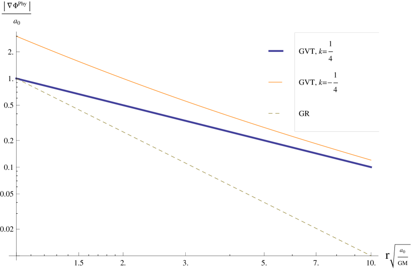
(a) The GravitoElectric Field strength

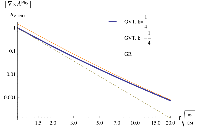
(b) The GravitoMagnetic Field strength

Figure 1: The GravitoElectroMagnetism of a spherical static mass distribution in the Einstein-Hilbert theory (GR) and the Gauge Vector Tensor theory (GVT).

Eq. (9.14) for $\kappa=\frac{1}{4}$ is the ordinary MOND modification of the Newtonian field capable of resolving the missing mass problem in galaxies and reproducing the Tully-Fisher relation [23]. This suggests to set

$$\kappa=\frac{1}{4}\,.$$ (9.16)

Fig. 1 depicts the magnitude of (9.14), and the magnitude of (9.15) for $J.r=0$ for two values of $k$ and

$$B_{MOND}=\frac{G|J|a_{0}^{\frac{3}{2}}}{2c^{2}(GM)^{\frac{3}{2}}}\,.$$ (9.17)

We see that the fall off of the gravitomagnetic field strengths of GVT in its MOND regime is $r^{-2}$ while that of the Einstein-Hilbert theory is $r^{-3}$. The gravitomagnetic field is enhanced in the deep MOND regime.

The equations for the Newtonian potential and the gravitomagnetic field of the $\Lambda$CDM theory read

$$\nabla^{2}\Phi = 4\pi G(\rho+\rho_{\text{Dark}})\,,$$ (9.18)

$$\nabla^{2}\vec{A} = \frac{16\pi G}{c^{2}}(\vec{j}+\vec{j}_{\text{Dark}})\,,$$ (9.19)

where $\rho_{\text{Dark}}$ and $j_{\text{Dark}}$ are respectively the density and the angular velocity distributions of dark matter. The gravitomagnetic field strength that the $\Lambda$CDM theory predicts for a spherical spinning galaxy at its edge then follows

$$\nabla\times\vec{A}_{\Lambda\text{CDM}} = \frac{G}{2c^{2}}(\frac{J}{r^{3}}-3J.r\frac{\vec{r}}{r^{5}})\,.$$ (9.20)

There exists no observational information available about the angular momentum distribution of dark matter. The theoretical scenarios consider the dark matter halo as a cloud of a vanishing angular momentum [26]. We, additionally, observe that the difference between GVT (9.15) and $\Lambda$CDM (9.20) can not be assigned to the total angular momentum of the dark matter. We, therefore, conclude that measuring the gravitomagnetic force at the edge/beyond the edge of a galaxy refutes one of the GVT and dark paradigms and proves the other one. However the gravitomagnetic force at the edge of a galaxy is too small that one may not hope for its detection in the near future.

9.3 Post-MONDian regime

Due to (8.20) the post-MONDian field starts from

$$\frac{4\kappa}{\beta}\sqrt{\frac{GM}{a_{0}}}<r\,.$$ (9.21)

and continues to infinity. In the post-MONDian regime, the $\tilde{B}_{\mu}$ field starts to behave like the $B_{\mu}$ field. So the physical gravitomagnetism in this regime follows:

$$-\nabla\Phi^{\text{Phy}} = -\left(\frac{GM}{r^{3}}+(1-\beta)\frac{\sqrt{GMa_{0}}}{r^{2}}\right)\vec{r}\,,$$ (9.22)

$$\nabla\times\vec{A}^{\text{Phy}} = (1-\beta)\frac{G}{8c^{2}(GMa_{0})^{\frac{1}{2}}}(\frac{J}{r^{2}}-3J.r\frac{\vec{r}}{r^{4}})+\,\frac{G}{2c^{2}}(\frac{J}{r^{3}}-3J.r\frac{\vec{r}}{r^{5}})+O(\frac{1}{r^{4}})\,,$$ (9.23)

where $\beta$ is defined in (8.19). Since $\beta$ is smaller than one, the MONDian behavior of the GVT though is decreased continues to infinity.

We note that the post-MONian behavior of the GVT theory can be enforced to coincide to the Newtonian one by introducing one additional gauge field. Let $\hat{B}_{\mu}$ be introduced whose action is similar to that of $B_{\mu}$ where $(\kappa,l)$ is replaced by $(\hat{\kappa},\hat{l})$. The interested reader can check that

$$\kappa+\tilde{\kappa}+\hat{\kappa}=0\,,$$ (9.24)

makes the theory consistent with the Einstein-Hilbert action in the strong and Newtonian regimes while the condition of

$$\frac{\kappa}{l}+\frac{\tilde{\kappa}}{\tilde{l}}+\frac{\hat{\kappa}}{\hat{l}}=0\,,$$ (9.25)

causes the theory to be consistent with the Einstein-Hilbert theory in the post-MONDian regime. Such a simple extension indicates to an advantage of the GVT theory over its rivals.

10 Gravitomagnetic field in the Solar system

In the TeVeS and the AQUAL theories, in some points within the solar system the gravitational fields of the planets and the Sun and the galaxy cancel each other. Let these points be called the gravitational saddle points. Ref. [31] identifies the gravitational saddle points of the solar system. Ref. [32, 33, 34] suggest that an accurate tracking of a probe like the LISA path finder that passes through the MOND windows can prove or refute the AQUAL theory. Ref. [35] proposes that measuring the behavior of gravity in short distances within the MOND windows can prove or refute the AQUAL theory. Ref. [36] mentions that observing pulsars through the gravitational saddle point of the Sun and Jupiter can empirically constrain the interaction of light with the physics of MOND system. This section aims to study the physics within the GVT MOND windows of the Solar system. To this aim we will consider the largest MOND window. The subsection 10.1 reviews the MOND window of the AQUAL theory. Then the subsection 10.2 identifies the Sun-Jupiter MOND window of the GVT theory. The subsection 10.3 solves the GVT equations in the Sun-Jupiter MOND window.

10.1 MOND windows of the AQUAL theory

This section aims to study the MOND windows in the framework of the AQUAL theory. To this aim we shall consider the largest solar MOND window. We will consider the gravitational saddle point of the Sun-Jupiter system. We employ the two bodies approximation to the Sun-Jupiter system. This approximation suffices for our studies because including the effects of other solar planets and the gravitational field of the galaxy will not significantly change the size of the considered MOND window [31].

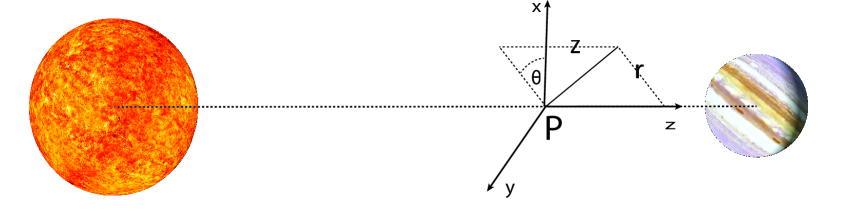
Figure 2: $P$ represents the gravitational saddle point of the Sun-jupiter system. We use the cylindrical coordinates around $P$ in order to solve the equations.

In this approximation the Newtonian gravitational field strength at the position $\vec{r}$ with respect to the center of the Sun reads:

$$g(\vec{r})=-\frac{GM_{\text{Sun}}}{|\vec{r}|^{3}}\vec{r}-\frac{GM_{\text{Jupiter}}}{|\vec{r}-\vec{d}|^{3}}(\vec{r}-\vec{d})\,.$$ (10.1)

where $\vec{d}$ is the vector connecting the center of the Sun to the center of the Jupiter. The gravitational saddle point $P$ is the point where in $g(\vec{r}_{p})=0$, so:

$$\vec{r}_{p}=\frac{\vec{d}}{1+\sqrt{\frac{M_{\text{Jupiter}}}{M_{\text{Sun}}}}}\,.$$ (10.2)

which means that the saddle point is $2.29\times 10^{7}km$ far away from the Jupiter. We would like to study the physics around the gravitational saddle point. We, therefore, taylor-expand the gravitational field around the saddle point:

$$\vec{r} = \vec{r}_{p}+\epsilon\delta r\,,$$ (10.3)

$$\delta r = \rho\hat{\rho}+z\hat{z}\,,$$ (10.4)

$$\vec{g}(\vec{r}) = 0+\alpha(2z\hat{z}-\rho\hat{\rho})+O(z^{2},\rho^{2})\,,$$ (10.5)

where fig. 2 depicts the chosen cylindrical coordinate and

$$\alpha\,=\,\frac{G}{d^{3}}\frac{\left(\sqrt{M_{\text{Sun}}}+\sqrt{M_{\text{Jupiter}}}\right)^{4}}{\sqrt{M_{\text{Sun}}M_{\text{Jupiter}}}}=1.084\times 10^{-14}s^{-2}.$$ (10.6)

The magnitude of the gravitoelectric field strength around the gravitational saddle point then follows:

$$|\vec{g}(\vec{r})|\,=\,0+\alpha\epsilon\sqrt{4z^{2}+\rho^{2}}+O(z^{2},\rho^{2})\,,$$ (10.7)

The AQUAL type MOND window is where

$$|\vec{g}(\vec{r})|<a_{0}.$$ (10.8)

So it is an ellipsoid with semi-axes of length

$$a = \frac{a_{0}}{2\alpha}\,=\,4.6~{}km\,,$$ (10.9a)

$$b = \frac{a_{0}}{\alpha}\,=\,9.2~{}km\,,$$ (10.9b)

$$c = \frac{a_{0}}{\alpha}\,=\,9.2~{}km\,.$$ (10.9c)

10.2 MOND windows of the GVT theory

The Newtonian regime of the GVT theory ends at

$$|\frac{l^{2}}{4}B_{\mu\nu}B^{\mu\nu}|=\frac{l^{2}}{2}\left(|\nabla B_{0}|^{2}-|\nabla\times\vec{B}|^{2})\right) = 1\,,$$ (10.10)

where $B$ is given in (6.20) and the unit of $c=1$ is used. Utilizing (10.1), $B_{0}$ in the Solar system reads

$$\nabla B_{0}(\vec{r})=4k\vec{g}(\vec{r})=-4\kappa\left(\frac{GM_{\text{Sun}}}{|\vec{r}|^{3}}\vec{r}+\frac{GM_{\text{Jupiter}}}{|\vec{r}-\vec{d}|^{3}}(\vec{r}-\vec{d})\right)\,.$$ (10.11)

The rotation of the Sun and Jupiter around their axes as well as the motion of the center of the mass of the Jupiter around the Sun contribute to the gravitomagnetic field strength in the Solar system:

$$\nabla\times\vec{A}_{\text{Jupiter}} = \frac{G}{2c^{2}}\left(\frac{\vec{J}_{J}}{(d-r)^{3}}-3\vec{J}_{J}.(\vec{d}-\vec{r})\frac{\vec{d}-\vec{r}}{|\vec{d}-\vec{r}|^{5}}\right)\,,$$ (10.12a)

$$\nabla\times\vec{A}_{\odot} = \frac{G}{2c^{2}}\left(\frac{\vec{J}_{\odot}}{r^{3}}-3\vec{J}_{\odot}.\vec{r}\frac{\vec{r}}{r^{5}}\right)\,,$$ (10.12b)

$$\nabla\times\vec{A}_{\text{Jupiter}}^{\text{Orbital}} = \frac{GM_{\text{Jupiter}}}{c^{2}|\vec{r}-\vec{d}|^{3}}\vec{v}_{cm}\times(\vec{r}-\vec{d})\,,$$ (10.12c)

where $J_{\odot}$ and $J_{J}$ are the angular momentum of the Sun and Jupiter while $v_{cm}$ is the velocity of the center of the mass of Jupiter with respect to the Sun. Utilizing (10.1) now leads to:

$$\nabla\times\vec{B} = \kappa(\nabla\times\vec{A}_{\text{Jupiter}}+\nabla\times\vec{A}_{\odot}+\nabla\times\vec{A}_{\text{Jupiter}}^{\text{Orbital}})\,,$$ (10.13)

Eq. (10.10), (10.11) and (10.13) identifies the boundary of the GVT MOND window of the Sun-Jupiter system in the two bodies approximation to the Solar system. This is the boundary of the MOND window with the Newtonian regime. Let it be highlighted that including the effects of other solar planets will not significantly change the size of this MOND window [31].

Since $k\approx O(1)$, the eq. (8.8) implies that $l\approx O(10^{26}m)$. Recalling that the gravitomagnetic field strength is weaker than the gravitoelectric field strength, (10.10) then implies that the GVT MOND window is not far away from the gravitational saddle point given in (10.2). To go further we approximate the angular momentum of the Sun and Jupiter to:

$$J_{\odot} = 1.92\times 10^{41}kgm^{2}s^{-1}\hat{x}\,,$$ (10.14)

$$J_{J} = 6.9\times 10^{38}kgm^{2}s^{-1}\hat{x}\,,$$ (10.15)

$$v_{cm} = d\frac{2\pi}{T}\hat{y}\,,$$ (10.16)

where $\hat{x}$ and $\hat{y}$ are presented in fig. 2 and $T$ is the orbital period of the Jupiter around the Sun:

$$T=4331.6~{}\mbox{days}\,.$$ (10.17)

We see that the magnitudes of the gravitomagnetic fields presented in (10.12) at $\vec{r}_{p}$ (and as well as its neighborhood) given in (10.2) read:

$$c\nabla\times A^{Sun}_{rotation} = \frac{G}{2c}\frac{J_{Sun}}{r^{3}_{p}}\hat{x}\,=1.05\times 10^{-13}\frac{m}{s^{2}}\hat{x},$$ (10.18a)

$$c\nabla\times A^{Jupiter}_{rotation} = \frac{G}{2c}\frac{J_{Jupiter}}{(d-r_{p})^{3}}\,=\,1.27\times 10^{-11}\frac{m}{s^{2}}\hat{x}\,,$$ (10.18b)

$$c\nabla\times A^{Jupiter}_{\text{orbital}} = \frac{G}{c}\frac{M_{\text{Jupiter}}}{d-r_{p}}\frac{2\pi}{T}\,\hat{z}=3.10\times 10^{-10}\frac{m}{s^{2}}\hat{x}\,,$$ (10.18c)

which in turn result

$$c^{2}|\nabla\times B|^{2}\approx 10.41\,\kappa^{2}\,a_{0}^{2}\,,$$ (10.19)

where (4.15) and (10.13) are used. Inserting (10.19) into (10.10) and expressing $l$ in term of $a_{0}$ by (8.8), and utilizing (10.11) yields

$$|g(r)|=a_{0}\sqrt{\frac{1}{256\kappa^{4}}+0.65}\,.$$ (10.20)

Notice that eq. (10.5) decribes the Newtonian gravitational field strength around $\vec{r}_{p}$. Now comparing (10.19) with (10.8) and (10.9) results that the GVT MOND window is an ellipsoid with semi-major axes of

$$(\tilde{a},\tilde{b},\tilde{c})=\sqrt{\frac{1}{256\kappa^{4}}+0.65}~{}\frac{a_{0}}{\alpha}(\frac{1}{2},1,1)\,.$$ (10.21)

The GVT MOND window is larger than the AQUAL MOND window for $|k|<0.325$.

The post MONDian regime resides inside the GVT MOND windows. The post MONDian regime is an ellipsoid with semi axes of

$$(\tilde{\tilde{a}},\tilde{\tilde{b}},\tilde{\tilde{c}})=\,\beta^{2}(\tilde{a},\tilde{b},\tilde{c}),$$ (10.22)

where $\beta$ is given in (8.19). Note that $\tilde{l}$ is the scale wherein $\tilde{B}$ starts its MONDian behavior. We assume that $\beta\ll 1$. This makes the post MONDian region of the Solar system sufficiently small to practically be ignored.

10.3 Gravitomagnetism inside the Sun-Jupiter GVT MOND window

The physical GravitoElectroMagnetism in the GVT theory receives contribution from the metric and the gauge fields, as stated in the eq. (7.8). The contribution of the metric to GEM inside the GVT MOND windows follows from (10.5) and (10.18):

$$-\nabla\Phi_{EH} = 0+\alpha(2z\hat{z}-\rho\hat{\rho})\,,$$ (10.23a)

$$\nabla\times A_{EH} = 3.22\times 10^{-10}\frac{m}{s^{2}}\hat{x}\,.$$ (10.23b)

The contribution of the $\tilde{B}$ follows from (8.5):

$$-\nabla\tilde{B}_{0} = -4\kappa\alpha(2z\hat{z}-\rho\hat{\rho})\,,$$ (10.24a)

$$\nabla\times\tilde{B}_{i} = -3.22\kappa\times 10^{-10}\frac{m}{s^{2}}\hat{x}\,.$$ (10.24b)

We should solve (9.4) in order to find the contribution of $B_{\mu}$. The solution of (9.4) can be expressed in term of (10.23):

$$\frac{\sqrt{||\nabla B_{0}|^{2}-|\nabla\times\vec{B}|^{2}|}}{a_{0}}\nabla B_{0} = -\alpha(2z\hat{z}-\rho\hat{\rho})+\nabla\times\vec{\tilde{h}}\,,$$ (10.25a)

$$\frac{\sqrt{||\nabla B_{0}|^{2}-|\nabla\times\vec{B}|^{2}|}}{a_{0}}\nabla\times\vec{B} = 3.22a_{0}\hat{x}+\nabla\tilde{h}\,,$$ (10.25b)

where $$\vec{\tilde{h}} \nabla\tilde{h}$$ and solve the following consistency equations:

$$\nabla\times\nabla B_{0} = \nabla\times\frac{-\alpha(2z\hat{z}-\rho\hat{\rho})+\nabla\times\vec{\tilde{h}}}{\sqrt{||\nabla B_{0}|^{2}-|\nabla\times\vec{B}|^{2}|}}=0\,,$$ (10.25c)

$$\nabla.\nabla\times\vec{B} = \nabla.\frac{3.22a_{0}\hat{x}+\nabla\tilde{h}}{\sqrt{||\nabla B_{0}|^{2}-|\nabla\times\vec{B}|^{2}|}}=0\,.$$ (10.25d)

We first look at part of the GVT MOND window wherein

$$|\nabla\times\vec{B}|^{2}>|\nabla B_{0}|^{2}\,,$$ (10.26)

where (10.25) can be approximated to:

$$\frac{|\nabla\times\vec{B}|}{a_{0}}\nabla B_{0} = -\alpha(2z\hat{z}-\rho\hat{\rho})+\nabla\times\vec{\tilde{h}}\,,$$ (10.27a)

$$\frac{|\nabla\times\vec{B}|}{a_{0}}\nabla\times\vec{B} = 3.22a_{0}\hat{x}+\nabla\tilde{h}\,,$$ (10.27b)

$$\nabla\times\frac{-\alpha(2z\hat{z}-\rho\hat{\rho})+\nabla\times\vec{\tilde{h}}}{|\nabla\times\vec{B}|} = 0\,,$$ (10.27c)

$$\nabla.\frac{3.22a_{0}\hat{x}+\nabla\tilde{h}}{|\nabla\times\vec{B}|} = 0\,.$$ (10.27d)

Eq. (10.27) is solved by

$$\nabla\times\vec{B} = 1.79a_{0}\hat{x}\,,$$ (10.28a)

$$\nabla{B}_{0} = -0.55\alpha(2z\hat{z}-\rho\hat{\rho})\,,$$ (10.28b)

$$\tilde{h} = \vec{\tilde{h}}=0\,.$$ (10.28c)

The condition of (10.26) applied on (10.28) gives

$$\sqrt{4z^{2}+\rho^{2}}<3.25\frac{a_{0}}{\alpha}\,,$$ (10.29)

Since the boundary of the GVT MOND window is given by (10.19), the eq. (10.29) holds true in whole of the GVT MOND window provided that

$$a_{0}\sqrt{\frac{1}{256\kappa^{4}}+0.65}<3.25a_{0}~{}~{}\to~{}~{}0.14<|\kappa|.$$ (10.30)

Notice that when $|\kappa|<0.14$ then (10.28) is not valid in a shell adjacent to the boundary of the MOND window. The physical GEM follows from (7.8), (10.23), (10.24) and (10.28):

$$\nabla\Phi_{Phy}=\nabla(\Phi_{EH}+B_{0}+\tilde{B}_{0})=4(0.39-\kappa)\nabla\Phi_{EH}\,,$$ (10.31a)

$$\nabla\times\vec{A}_{Phy}=\nabla(A_{EH}+\vec{B}+\vec{\tilde{B}})=(1.56-\kappa)\nabla\times\vec{A}_{EH}\,,$$ (10.31b)

We next look at part of the GVT MOND window that holds

$$|\nabla B_{0}|^{2}>|\nabla\times\vec{B}|^{2}\,.$$ (10.32)

wherein (10.25) can be approximated to:

$$\frac{|\nabla{B}_{0}|}{a_{0}}\nabla B_{0} = -\alpha(2z\hat{z}-\rho\hat{\rho})+\nabla\times\vec{\tilde{h}}\,,$$ (10.33a)

$$\frac{|\nabla B_{0}|}{a_{0}}\nabla\times\vec{B} = 3.22a_{0}\hat{x}+\nabla\tilde{h}\,,$$ (10.33b)

$$\nabla\times\frac{-\alpha(2z\hat{z}-\rho\hat{\rho})+\nabla\times\vec{\tilde{h}}}{|\nabla B_{0}|} = 0\,,$$ (10.33c)

$$\nabla.\frac{3.22a_{0}\hat{x}+\nabla\tilde{h}}{|\nabla B_{0}|} = 0\,.$$ (10.33d)

Eq. (10.33) represents a set of second order partial differential equations. It can be analytically solved around $z\approx 0$ or $\rho\approx 0$ where it holds (10.28c). The solution around $z\approx 0$ reads

$$\nabla B_{0} = +\sqrt{\alpha a_{0}\rho}\,\hat{\rho}+O(z)=\sqrt{\frac{a_{0}}{\alpha\rho}}\nabla\Phi_{EH}+O(z)\,,$$ (10.34a)

$$\nabla\times\vec{B} = 3.22(\frac{a_{0}}{\alpha\rho})^{\frac{1}{2}}a_{0}\hat{x}+O(z)=\sqrt{\frac{a_{0}}{\alpha\rho}}\nabla\times A_{EH}+O(z)\,,$$ (10.34b)

while the solution around $\rho\approx 0$ follows

$$\nabla B_{0} = -\text{Sign}(z)\sqrt{2\alpha a_{0}z}\,\hat{z}+O(\rho)=\sqrt{\frac{a_{0}}{2\alpha z}}\nabla\Phi_{EH}+O(\rho)\,,$$ (10.35a)

$$\nabla\times\vec{B} = 3.22(\frac{a_{0}}{2\alpha z})^{\frac{1}{2}}a_{0}\hat{x}+O(\rho)=\sqrt{\frac{a_{0}}{2\alpha z}}\nabla\times A_{EH}+O(\rho)\,.$$ (10.35b)

Eq. (10.34) and (10.35) are respectively valid in

$$3.22a_{0} <\alpha\rho< \sqrt{\frac{1}{256\kappa^{4}}+0.65}\,a_{0}\,,$$ (10.36a)

$$3.22a_{0} <2\alpha z< \sqrt{\frac{1}{256\kappa^{4}}+0.65}\,a_{0}\,,$$ (10.36b)

wherein the upper bound is the boundary of the MOND regime and the lower bound is (10.32) written for (10.34) and (10.35). This means that (10.34) and (10.35) are valid solutions provided that

$$|\kappa|<0.14,$$ (10.37)

which is complementary to (10.30). Eq. (10.34) and (10.35) describe the behavior of $B$ in a shell adjacent to the boundary of the MOND window that eq. (10.28) is not valid in. They present an enhancement for the gravitomagnetic and gravitoelectric field strengths. However due to the lower bound in (10.36), the enhancement is bounded and is not akin to that of naive extension of MOND to the gravitomagnetic force: eq. (A.10) for $\rho\to 0$ or $z\to 0$.

The physical GEM following from (7.8), (10.23), (10.24) for (10.34) reads:

$$\nabla\Phi_{Phy}=\left(1-4\kappa+\sqrt{\frac{a_{0}}{2\alpha z}}\right)\nabla\Phi_{EH}+O(\rho)\,,$$ (10.38a)

$$\nabla\times\vec{A}_{Phy}=\left(1-\kappa+\sqrt{\frac{a_{0}}{2\alpha z}}\right)\nabla\times\vec{A}_{EH}+O(\rho)\,.$$ (10.38b)

While (10.35) yields:

$$\nabla\Phi_{Phy}=\left(1-4\kappa+\sqrt{\frac{a_{0}}{\alpha\rho}}\right)\nabla\Phi_{EH}+O(z)\,,$$ (10.39a)

$$\nabla\times\vec{A}_{Phy}=\left(1-\kappa+\sqrt{\frac{a_{0}}{\alpha\rho}}\right)\nabla\times\vec{A}_{EH}+O(z)\,.$$ (10.39b)

Eq. (10.38) and (10.39) respectively describe the GEM around $z\approx 0$ and $\rho\approx 0$ for the GVT MOND regime that holds (10.32). The physical GEM in other points will be identified after solving (10.27) and choosing the boundary conditions on $\vec{\tilde{h}}$ and $\tilde{h}$ such that the general solution reduces to (10.38) and (10.39) respectively for $z\approx 0$ and $\rho\approx 0$.

The accurate tracking of a probe passing through the MOND windows is the simplest way to test the physics of the Solar MOND windows. For $k\geq 0.14$, a probe that passes through the Sun-Jupiter GVT MOND window experiences the following anomalous acceleration:

$$\vec{a}_{\text{anomaly}}\,=\,-(0.56-4\kappa)\nabla\Phi_{EH}+(0.56-\kappa)\frac{\vec{v}}{c}\times\nabla\times\vec{A}_{EH}\,,$$ (10.40)

where $\vec{v}$ is the velocity of the probe with respect to the Sun and we have utilized (2.16) and (10.31). For $k<0.14$, a probe moving in $z=0$ or $\rho=0$ experiences the following anomalous acceleration in the regime of (10.36)

$$\vec{\tilde{a}}_{\text{anomaly}}\,=\,-\left(-4\kappa+\sqrt{\frac{a_{0}}{|\nabla\Phi_{EH}|}}\right)\nabla\Phi_{EH}+\left(-\kappa+\sqrt{\frac{a_{0}}{|\nabla\Phi_{EH}|}}\right)\frac{v}{c}\times\nabla\times\vec{A}_{EH}\,,$$ (10.41)

while experiences the anomalous acceleration given by (10.40) in the rest of the GVT MOND window. We observe that for the peculiar value of $k=0.14$, a slow moving probe ($\frac{|\vec{v}|}{c}\ll 1$) will not experience an anomalous acceleration inside the Sun-Jupiter MOND window. This peculiar value of $k$ is not universal and depends on the details of the considered MOND window. In order to refute the GVT theory by the accurate tracking of a probe that passes through the MOND windows, therefore, we must either

• increase the precision such that the anomalous acceleration in the gravitomagnetic force be observed,

• or to track probes in different MOND windows.

Observing an anomaly in a single MOND window, however, refutes the Einstein-Hilbert theory and favors the GVT, TeVeS or the Moffat’s theory. The GVT theory, so far, is the only generally covariant theory that also predicts an anomaly in the gravitomagnetic field inside the MOND window.

11 Conclusion and outlook

We have introduced the Gauge Vector Tensor theory: a generally covariant theory of gravity composed of a pseudo Riemannian metric and two $U(1)$ gauge connections that reproduces MOND in the limit of very weak gravitational fields while remains consistent with the Einstein-Hilbert gravity in the limit of strong and Newtonian gravitational fields. The nonlinearity introduced by the GVT theory to reproduce the MOND behavior resides only inside the MOND regime and it does not propagates to the strong regime of gravity. This is a clear advantage of the GVT theory over the Bekenstein’s Tensor-Vector-Scaler theory [5]. We have been motivated to introduce the GVT theory after uplifting the GravitoElectroMagnetism approximation to gravity to the Milgrom’s MOND theory [18].

We have illustrated that the gravitomagnetic force at the edge of a galaxy can be in accord with either GVT or $\Lambda$CDM but not both. We also have studied the physics of the GVT theory around the gravitational saddle point of the Sun and Jupiter system. We have noticed that the conclusive refusal of the GVT theory demands measuring either both of the gravitoelectric and gravitomagnetic fields inside the Sun-Jupiter MOND window, or the gravitoelectric field inside two different solar GVT MOND windows. The GVT theory, however, can be favored by observing an anomaly in the gravitoelectric field inside a single MOND window.

We also need to study the cosmology and the gravitational lensing of the GVT theory. Let it be hasten that, as shown in section 6, the GVT theory is an extension of the Moffat’s Scalar-Tensor-Vector theory [25]. We, therefore, envisage that it inherits most of the merits of the Moffat’s theory in describing the gravitational lensing and cosmology. We, however, accomplish this study elsewhere.

Appendix A Naive extension of MOND to the GravitoMagnetic Force

Modified Newtonian Dynamics (MOND) provides an alternative approach to the missing mass problem in galaxies. It assumes that the newtonian dynamics is governed by

$$\vec{F}=mf(\frac{|a|}{a_{0}})\vec{a}$$ (A.1)

where $F$ is the force exerted on the center of the mass of the object, $a$ is the acceleration of the object with respect to the cosmological frame wherein the CMB is uniform, and $a_{0}$ is given in (4.15). MOND coincides to the Newtonian dynamics in large accelerations:

$$\lim_{x\to\infty}f(x)=1\,.$$ (A.2)

Note that $x\ll 1$ is called the Newtonian regime of the MOND theory. To account for the missing mass problem, it is required that

$$f(x)=x\,\qquad\mbox{for}~{}x\leq 1\,.$$ (A.3)

Note that $x\leq 1$ is called the MOND regime.

The gravitational force extorted on a slow moving particle (the test particle) of mass $m$ and velocity $\vec{v}$ in the GravitoElectroMagnetism approximation to gravity follows from (2.16)

$$F=m(-\nabla\phi+\vec{v}\times\nabla\times A)$$ (A.4)

where $\phi$ is the Newtonian gravitational field (the gravitoelectric field) and $\nabla\times A$ is the gravitomagnetic field strength. The gravitoelectromagnetic fields of a spherical static mass distribution read

$$\phi(r) = -\frac{GM}{r}\,,$$ (A.5a)

$$A(r) = -\frac{2G}{c^{2}r^{3}}\vec{J}\times\vec{r}\,,$$ (A.5b)

where $r$ is the distance from the center of the mass distribution (the source), $M$ is its total mass and $J$ represents the total angular momentum of the source.

The GEM approximation of the Newtonian regimes of the MOND paradigm coincide to that of the the Einstein-Hilbert gravity. The story, however, changes in the MOND regime of the theory. The MOND regime holds

$$-\nabla\phi+\vec{v}\times\nabla\times A=\frac{|a|}{a_{0}}a\,.$$ (A.6)

which is a non-linear second order differential equation for the position of the test particle. Eq. (A.6) results

$$\frac{|a|^{4}}{a_{0}^{2}}=|-\nabla\phi+\vec{v}\times\nabla\times A|^{2}$$ (A.7)

using which in (A.6) returns

$$a=\sqrt{\frac{a_{0}}{|-\nabla\phi+\vec{v}\times\nabla\times A|}}(-\nabla\phi+\vec{v}\times\nabla\times A)\,,$$ (A.8)

Around galaxies the gravitoelectric force is much larger than the gravitomagnetic one. We therefore can taylor expand (A.8) in term of $v$ and obtain:

$$a=\sqrt{\frac{a_{0}}{|\nabla\phi|}}\left(-\nabla\phi+\vec{v}\times\nabla\times A+\nabla\phi\frac{\nabla\phi.\vec{v}\times(\nabla\times A)}{|\nabla\phi|^{2}}\right)+O(v^{2})\,.$$ (A.9)

The first two terms in the r.h.s of (A.9) can be interpreted as the gravitoelectric and gravitomagnetic force in the the MOND regime:

$$E_{\mbox{\tiny MOND}} = \sqrt{\frac{a_{0}}{|\nabla\phi|}}\nabla\phi\,,$$ (A.10a)

$$B_{\mbox{\tiny MOND}} = \sqrt{\frac{a_{0}}{|\nabla\phi|}}\nabla\times A\,.$$ (A.10b)

Since the MOND regime holds $|\nabla\phi|<a_{0}$ then we observe an enhancement in the gravitoelectric and gravitomagnetic field strength. The enhancement factor is $\sqrt{\frac{a_{0}}{|\nabla\phi|}}$. The last term in the r.h.s of (A.9) is a new kind of gravitational force acting on the test particle. This new force can be expressed through

$$F=m\nabla\phi\frac{\vec{v}.\nabla\phi\times(\nabla\times A)}{|\nabla\phi|^{2}}\sqrt{\frac{a_{0}}{|\nabla\phi|}}\,,$$ (A.11)

Two understand a possible meaning of this force let us consider the gravitoelectric and gravitomagnetic field strength of a spherical static mass distribution given in (9.1). The new force then simplifies to

$$F=\sqrt{\frac{4Ga_{0}}{Mc^{4}}}\,\frac{\vec{v}.\vec{r}\times J}{r^{3}}\hat{r}$$ (A.12)

Note that $J$ is the total angular momentum of the mass distribution and it is proportional to the total mass. Therefore the limit of $M\to 0$ in the eq. (A.12) exists. This force is in the direction of the gravitoelectric force and is less than it. So it would not significantly change the physics. We, however, take the position that this new force is an artifact of naively applying the MOND to the gravitomagnetic force.

References

- [1] B. Famaey and S. McGaugh, “Modified Newtonian Dynamics (MOND): Observational Phenomenology and Relativistic Extensions,” Living Rev. Rel. 15 (2012) 10 [arXiv:1112.3960 [astro-ph.CO]].
- [2] P. Kroupa, M. Pawlowski and M. Milgrom, “The failures of the standard model of cosmology require a new paradigm,” arXiv:1301.3907 [astro-ph.CO].
- [3] B. Famaey and S. McGaugh, “Challenges for Lambda-CDM and MOND,” arXiv:1301.0623 [astro-ph.CO].
- [4] Q. Exirifard, “Phenomenological covariant approach to gravity,” Gen. Rel. Grav. 43, 93 (2011) [arXiv:0808.1962 [gr-qc]].
- [5] J. D. Bekenstein, “Relativistic gravitation theory for the MOND paradigm,” Phys. Rev. D 70 (2004) 083509 [Erratum-ibid. D 71 (2005) 069901] [arXiv:astro-ph/0403694].
- [6] H. F. M. Goenner, “On the History of Geometrization of Space-time: From Minkowski to Finsler arXiv:0811.4529 [gr-qc].
- [7] John Archibald Wheeler, “ Geons”, Phys. Rev. 97 (1955) 511.
- [8] R. Penrose, Rev. Nuovo Cimento, 1 (1969) (Special Number), 252.
- [9] J. Lense and H. Thirring, Phys. Zeits. 19, 156 (1918).
- [10] L. Iorio, H. I. M. Lichtenegger, M. L. Ruggiero and C. Corda, “Phenomenology of the Lense-Thirring effect in the Solar System,” Astrophys. Space Sci. 331 (2011) 351 [arXiv:1009.3225 [gr-qc]].
- [11] T. Padmanabhan, Gravitation: Foundations and Frontiers, Cambridge University Press, www.cambridge.org/9780521882231 .
- [12] Pugh, G.E.: WSEG Research Memorandum No. 11 (1959).
- [13] L. I. Schiff, “Possible New Experimental Test of General Relativity Theory," Phys. Rev. Lett. 4, 215 (1960).
- [14] C. W. F. Everitt et al., “Gravity Probe B: Final Results of a Space Experiment to Test General Relativity,” Phys. Rev. Lett. 106 (2011) 221101, arXiv:1105.3456 [gr-qc].
- [15] A. Tartaglia, “Experimental determination of gravitomagnetic effects by means of ring lasers,” arXiv:1212.2880 [gr-qc].
- [16] Ignazio Ciufolini, Erricos C. Pavlis, John Ries, Rolf Koenig, Giampiero Sindoni, Antonio Paolozzi and Hans Newmayer, “Gravitomagnetism and Its Measurement with Laser Ranging to the LAGEOS Satellites and GRACE Earth Gravity Models”, General Relativity and John Archibald Wheeler Astrophysics and Space Science Library, Volume 367 (2010) pp 371-434 .
- [17] T. W. Murphy, Jr., K. Nordtvedt and S. G. Turyshev, “The Gravitomagnetic Influence on Gyroscopes and on the Lunar Orbit,” Phys. Rev. Lett. 98 (2007) 071102 [gr-qc/0702028].
- [18] M. Milgrom, “A modification of the Newtonian dynamics as a possible alternative to the hidden mass hypothesis”, Astrophys. J. 270 (1983) 365; M. Milgrom, “A modification of the Newtonian dynamics: Implications for galaxies”, Astrophys. J. 270 (1983) 371.
- [19] J. Bekenstein, M. Milgrom, “Does the missing mass problem signal the breakdown of Newtonian gravity?” Astrophysical J. 286, (1984) 7.
- [20] B. Famaey and J. Binney, “Modified Newtonian dynamics in the Milky Way”, Mon. Not. Roy. Astron. Soc. 363 (2005) 603 [arXiv:astro-ph/0506723]:
- [21] J. D. Bekenstein, “The modified Newtonian dynamics-MOND-and its implications for new physics”, arXiv:astro-ph/0701848; K. G. Begeman, A. H. Broeils and R. H. Sanders, “ Extended rotation curves of spiral galaxies: Dark haloes and modified dynamics”, Mon. Not. Roy. Astron. Soc. 249 (1991) 523.
- [22] T. Jacobson, “When is g(tt) g(rr) = -1?,” Class. Quant. Grav. 24, 5717 (2007) [arXiv:0707.3222 [gr-qc]].
- [23] R. B. Tully and J. R. Fisher, “A new method of determining distances to galaxies,” Astron. Astrophys. 54 (1977) 661.
- [24] Q. Exirifard, “GravitoMagnetic Field in Tensor-Vector-Scalar Theory,” JCAP 1304 (2013) 034 [arXiv:1111.5210 [gr-qc]].
- [25] J. W. Moffat, “Scalar-tensor-vector gravity theory,” JCAP 0603 (2006) 004 [gr-qc/0506021].
- [26] P. Bhattacharjee, S. Chaudhury, S. Kundu and S. Majumdar, “Sizing-up the WIMPs of Milky Way : Deriving the velocity distribution of Galactic Dark Matter particles from the rotation curve data,” arXiv:1210.2328 [astro-ph.GA].
- [27] Gunnar Randers, On an Asymmetrical Metric in the Four-Space of General Relativity Phys. Rev. 59, 195-199 (1941): DOI:10.1103/PhysRev.59.195 .
- [28] Z. Chang and X. Li, Modified Newton’s gravity in Finsler Space as a possible alternative to dark matter hypothesis, Phys. Lett. B 668, 453 (2008) [arXiv:0806.2184 [gr-qc]].
- [29] Z. Chang and X. Li, Modified Friedmann model in Randers-Finsler space of approximate Berwald type as a possible alternative to dark energy hypothesis, Phys. Lett. B 676, 173 (2009) [arXiv:0901.1023 [gr-qc]].
- [30] X. Li and Z. Chang, The Spacetime structure of MOND with Tully-Fisher relation and Lorentz invariance violation, arXiv:1204.2542 [gr-qc].
- [31] P. Galianni, M. Feix, H. Zhao and K. Horne, “Testing quasilinear modified Newtonian dynamics in the Solar System,” Phys. Rev. D 86 (2012) 044002 [arXiv:1111.6681 [astro-ph.EP]].
- [32] J. Bekenstein and J. Magueijo, “Mond habitats within the solar system", Phys. Rev. D 73 (2006) 103513 [astro-ph/0602266].
- [33] A. Mozaffari, “Testing Different Formulations of MOND Using LISA Pathfinder", arXiv:1112.5443 [astro-ph.CO].
- [34] J. Magueijo and A. Mozaffari, “The case for testing MOND using LISA Pathfinder", Phys. Rev. D 85 (2012) 043527 [arXiv:1107.1075 [astro-ph.CO]].
-
[35]
Q. Exirifard,
“ Measuring gravitational behavior at short distances in space:
A local test for MOND/MOG” arXiv:1206.0173 [gr-qc]. - [36] Q. Exirifard, “Lunar system constraints on the modified theories of gravity,” arXiv:1112.4652 [gr-qc].