Searching for Saturn’s Dust Swarm: Limits on the size distribution of Irregular Satellites from km to micron sizes

Abstract

We describe a search for dust created in collisions between the Saturnian irregular satellites using archival Spitzer MIPS observations. Although we detected a degree scale Saturn-centric excess that might be attributed to an irregular satellite dust cloud, we attribute it to the far-field wings of the PSF due to nearby Saturn. The Spitzer PSF is poorly characterised at such radial distances, and we expect PSF characterisation to be the main issue for future observations that aim to detect such dust. The observations place an upper limit on the level of dust in the outer reaches of the Saturnian system, and constrain how the size distribution extrapolates from the smallest known (few km) size irregulars down to micron-size dust. Because the size distribution is indicative of the strength properties of irregulars, we show how our derived upper limit implies irregular satellite strengths more akin to comets than asteroids. This conclusion is consistent with their presumed capture from the outer regions of the Solar System.

1 Introduction

The Solar System’s irregular satellites are long thought to have undergone collisions. When only eight were known at Jupiter, Kessler (1981) showed that the collision time for objects in the prograde group was less than the Solar System’s age. More recently, the discovery of collisional families shows that collisions occurred in the past (Nesvorný et al., 2003). Further evidence lies with the relatively flat size distributions of large irregulars, which Bottke et al. (2010) show can be produced from initially steeper distributions by billions of years of collisional evolution. Their collisional evolution is thought to have begun when the irregulars were captured from cold icy regions of the Solar System (e.g. Nesvorný et al., 2007).

Though the Bottke et al. results are based on reproducing the size distribution of the known irregulars, the destruction of the largest objects must produce vast numbers of fragments. The fragments collide with each other, producing yet more fragments and so on down to dust. The known irregulars are just the largest objects in a continuous size distribution that extends down to the smallest grains that can survive on circumplanetary orbits. It is therefore inevitable that dust associated with irregular satellites exists at some level around the giant planets.

We recently made predictions of the level of this dust based on a collisional model and a simple prescription for the size distribution (Kennedy & Wyatt, 2011). However, these predictions are uncertain for several reasons. The many orders of magnitude between the 10–100km size of known objects and the smallest dust grains means that small differences in the slope of the assumed size distribution result in large differences in the level of dust. This slope depends on the strength law, which is uncertain. There may also be additional loss mechanisms that flatten the size distribution relative to theoretical predictions for a collisional cascade.

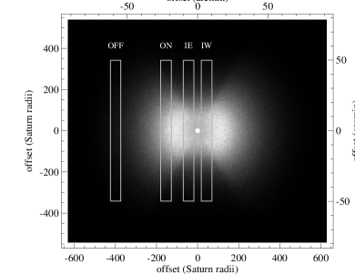
Figure 1: Simple model of Saturn’s irregular satellite dust cloud in Saturnian and sky coordinates (y=0 is the ecliptic). The scale is a linear stretch. Saturn’s position is marked by a dot (brightness not to scale). The boxes show the approximate position of the two Phoebe ring (ON,OFF) and two Iapetus (East,West) scans.

Detection of this dust is therefore important for several reasons. Primarily it would provide the strongest evidence yet that the known irregular satellites are just the tip of a continuous size distribution. Because the collisional lifetime of the dust is of order tens of millions of years, any existing dust must be continually replenished by destruction of larger objects, which implies ongoing destruction of objects of all sizes. Characterising the dust population is also important for understanding irregulars themselves, because the slope of the size distribution depends on their strength properties (O’Brien & Greenberg, 2003). More generally, the irregular satellites provide a rare chance to observe how the size distribution in a collisional cascade extrapolates from large objects down to dust, thus informing models used to model extrasolar debris disks.

Additional motivation comes from the existence of dust related to a single Saturnian irregular satellite; the Phoebe ring (Verbiscer et al., 2009). Impacts that launch grains from Phoebe are proposed as a way to feed the ring. Whether the impactor population is interplanetary, or belongs to a cloud of circumplanetary dust (i.e. due to irregulars) is not known. Detection of a dust cloud would provide compelling evidence in favour of the latter.

A simple way to estimate the spatial distribution of such a grain population is to assume that they follow the orbits of the observed irregulars, which yields a model for the surface brightness distribution of the dust cloud. Figure 1 shows this model for Saturn, made by generating a population of particles with random semi-major axes, eccentricities, and inclinations in the range derived for captured Saturn-centric orbits by Nesvorný et al. (2007). The scale shows that the cloud extends over a degree in each direction. The smaller vertical extent is the result of a lack of near-polar orbits, which are unstable due to Solar perturbations (Carruba et al., 2002; Nesvorný et al., 2003). The peak surface brightness predicted for Figure 1 is 1.25MJy/sr (Kennedy & Wyatt, 2011), but as noted above is uncertain.

Our aim here is to test this prediction for Saturn’s dust cloud using the 24$\mu$m Spitzer Space Telescope observations used to discover the Phoebe ring. The regions of sky covered by these observations relative to Saturn is also shown in Figure 1. The data cover a sufficiently wide region around Saturn to appear promising for a deeper look for a cloud of dust originating from the irregular satellites. In the next sections, we describe our efforts to extract a signal that can be compared with Figure 1.

2 Data

The Spitzer data (programmes 40840 and 50780) are described in Verbiscer et al. (2009) and their location in relation to Saturn is shown in Figure 1 (see also Verbiscer et al., 2009). For this study we use only the 24$\mu$m Multiband Imaging Photometer (MIPS, Rieke et al., 2004) data.

The Phoebe ring discovery data consist of a long image 128–180 $R_{\rm Sat}$ from Saturn (called ON, 18/2/2009), just inside the maximum extent of Phoebe’s orbit. To allow foreground and background subtraction, another image 400 $R_{\rm Sat}$ away was also taken (OFF, 10/2/2009). In addition, we found it necessary to use two images located much closer to Saturn (IAPETUS East and West, 28/6/2008) to characterise the point spread function (PSF).

Each image comprises two consecutive scans 1.5^∘ long taken approximately perpendicular to the ecliptic. Each scan is built from 178 individual basic calibrated data (BCD) images. The second scan is in the reverse direction to the first, but with a small offset so each pair of scans overlap by about half their width ($\sim$2.5 arcmin). Here, we worked with the scans rather than the combined images (see below). Before analysing the scans we remove point sources, Zodiacal foreground using the COBE/DIRBE Zodiacal cloud model of Kelsall et al. (1998), and mask a number of glint and diffraction artefacts that are present due to the proximity of Saturn to the field of view, particularly in the ON scan (see Verbiscer et al., 2009).

The zodiacal foreground subtraction does not account for all of the foreground in any of the scans because ecliptic dust components (e.g. asteroidal dust bands; Low et al., 1984; Grogan et al., 2001) are poorly characterised in this (or any) model. However, because the ON and OFF scans were taken about a week apart, we only expect an absolute offset due to the $\sim$9^∘ change in elongation. We expect the latitudinal structure to be similar, which is borne out by the data (see below).

Unfortunately, subtracting the OFF scan from the Iapetus scans cannot be justified due to the seven month time difference, and the resultant different Zodiacal structure. Instead the DIRBE model was scaled up by a factor 1.17 to bring the profiles to near-zero at the ends. Alternatively, a DC offset can be subtracted to give essentially the same result.

3 Analysis

The data analysis is split into two sections. First, we do the ON-OFF subtraction, which clearly shows excess surface brightness near Saturn. The two main possible causes of this signal are i) our proposed dust cloud, and ii) the far-field wings of the Spitzer PSF due to nearby Saturn (which is $\sim$15000Jy at 24$\mu$m, several thousand times greater than the MIPS 24$\mu$m saturation limit of $\sim$6Jy). In the second subsection, we use the Iapetus scans to characterise the PSF at large angular separations as a possible cause of the measured ON-OFF signal.

3.1 ON-OFF Subtraction

Based on Figure 1, we expect the cloud to vary smoothly over the 1.5^∘ scan with a Gaussian-like shape. For the ON-OFF subtraction to be valid and successful we are assuming that the dust cloud is not present in the OFF image, or is at a much lower level. The dust level must also vary over the ON image, because some constant offset is likely between the two images due to the elongation difference and poor characterisation of ecliptic dust, which could not definitely be attributed to dust associated with Saturn.

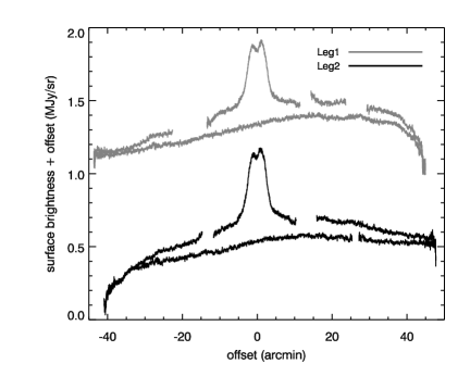
Figure 2: Zodiacal light subtracted median scan profiles. The x axis shows the approximate offset from the center of the Phoebe ring, visible as the enhancement in the ON scans. Gaps in the profiles are from masking out diffraction spikes and glints from Saturn. An arbitrary DC offset has been subtracted, with the Leg 1 data offset for clarity.

Profiles across the ON and OFF scans are shown in Figure 2. Each profile is a median collapse taken parallel to the long axis of a scan. Each pair has been scaled to give the same level at the profile ends. The ON scans are easily identifiable by the large bump in the middle due to the Phoebe ring. The corresponding leg of the OFF scan is shown below each ON scan. Ecliptic South is to the left, so Leg 1 is taken from right to left, and Leg 2 from left to right. The strong curvature at the beginning of each scan (at offset of +40 arcmin for Leg 1, at -40 arcmin for Leg 2) is due to a brief change in the detector bias applied just prior to the start of each scan. While the first five frames are usually disregarded in typical scan maps, Figure 2 shows that this artefact is repeatable and can be accounted for as long as the individual scans are used.

A positive trend towards ecliptic North (right) is apparent for all four scans, most likely due to a heliocentric dust band. Whether such a trend is likely can be gauged using Zodiacal model Subtracted Mission Averaged (ZSMA) COBE DIRBE maps. The ZSMA image of the region observed in the ON/OFF observations is shown in Figure 3, which makes it clear that the Zodiacal model is far from perfect in the ecliptic (see also Figure 2 of Kelsall et al., 1998). This image clearly shows residuals that are the result of a heliocentric dust band not included or not well characterised by the Kelsall et al. (1998) Zodiacal model. The most prominent band of excess brightness coincides with the North end of the MIPS scans, which is likely the cause of the observed increasing trend to the North end of the profiles (and perhaps some DC offset). We cannot simply subtract a profile based on this image because the COBE DIRBE maps comprise scans at a range of elongation angles.

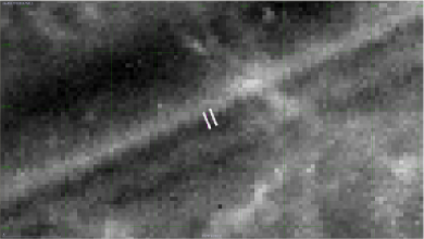
Figure 3: COBE DIRBE 25$\mu$m ZSMA image and MIPS ON/OFF scans (center, OFF is the left rectangle). The bright strip passing from lower left to upper right is parallel to the ecliptic, and shows excess surface brightness due to a poorly characterised heliocentric dust band.

As well as the obvious detection of the Phoebe ring, it is clear from Figure 2 that there is a difference that extends for nearly the entire length of the ON and OFF scans. This difference is shown in Figure 4. This figure also shows that the curvature due to the detector response at the start of each scan is removed fairly successfully. Also shown is a vertical cut through the dust model of Figure 1 at the position of the ON scan, scaled to match the observed profile. The signal is clearly real, and tantalising as a possible dust detection.

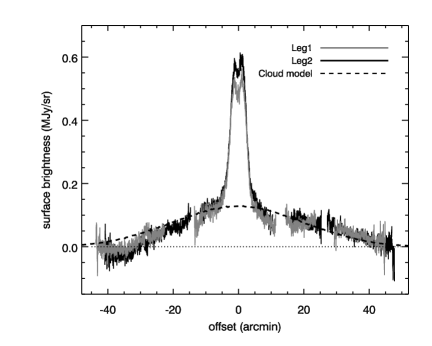
Figure 4: ON-OFF subtracted median scan profiles. The x axis shows the approximate offset from the center of the Phoebe ring.

3.2 PSF Characterisation

While there appears to be a real difference between the ON and OFF images, we need to consider the level of Spitzer’s PSF due to Saturn, which could result in a similar signal. The obvious way to estimate the level of the PSF is with the STinyTim PSF model. However, these PSFs are well characterised on the scale of a few minutes of arc, not the $\sim$degree scales that apply to these observations (J. Krist, priv. comm.). Therefore, we must use an empirical approach, made possible by the existence of the Iapetus scans. These scans are much closer to Saturn than the ON and OFF ones, and may therefore be suitable for deriving an empirical profile of surface brightness with radial distance from Saturn.

Of course the limitation of this approach is that the Iapetus scans may themselves have detected the dust cloud, so consistency between the ON-OFF and Iapetus profiles does not exclude the possibility of a dust cloud. Based on Figure 1, one might expect the level of dust to be lower in the Iapetus scans due to the non-spherical shape of the cloud, in which case any significant difference between radial profiles extracted from the Iapetus scans and the ON-OFF subtraction might be attributed to a dust cloud.

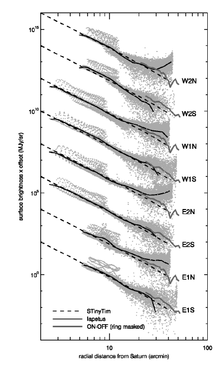
Figure 5: Median radial profiles derived from the Iapetus scans (dark solid lines) and STinyTim (dashed lines). Each scan is labelled according to whether it is East or West, Leg 1 or Leg 2, and North or South of a line along Saturn’s orbit. The solid grey lines are median radial profiles of the ON-OFF scans, with Leg 1 plotted over the South Iapetus profiles and Leg 2 plotted over the North Iapetus profiles. The grey background dots are actual pixel values from the scans plotted at their radial distance from Saturn.

Figure 5 shows median radial profiles of the two pairs of Iapetus scans, centered on Saturn’s position. The grey background dots are pixel values from the scans plotted at their radial distance from Saturn. Taking the median means that azimuthal structures such as diffraction spikes (visible at radii $\lesssim$10 arcmin) do not affect the profiles. The profiles are also separated into North and South of a line along Saturn’s orbit (solid lines), and are labelled as ‘E’ (East) and ‘W’ (West), with the scan legs following the same convention as the ON/OFF scans. Therefore the lowest profile in the Figure, ’E1S’, is the South part of Leg 1 of the Iapetus East scan.

The reason for separating the scans into North and South is apparent. All North scan profiles turn up around 30 arcmin from Saturn, likely due to the same dust band seen in the ON/OFF scans in Figure 2 but more pronounced. The difference is probably because the Iapetus scans were taken seven months earlier with a consequently different line of sight through the Zodiacal cloud, which unfortunately means we cannot use the OFF scan to remove the foreground as we did for the ON scan. This turn up is less pronounced in the Leg 1 (downward) scans (i.e. E1N and W1N), where the detector bias response (§2) at the beginning of a scan counteracts the turn-up.

Figure 5 also shows radial profiles derived from the ON-OFF subtracted scans (assuming axisymmetry, grey lines). Despite uncertainties introduced by the dust band, these profiles lie within the scatter of the Iapetus scans (i.e. sometimes above, sometimes below), so appear consistent with having the same origin. The dashed lines show a scaled STinyTim median radial profile, which also appear consistent with the Iapetus observations. The STinyTim model is well fitted by a power law $\propto r^{-3.1}$ at distances larger than 1 arcmin.

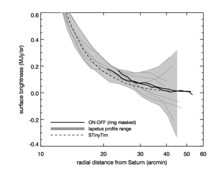
Figure 6: Median radial profiles derived from the Iapetus scans (grey swathe and dark grey lines) and STinyTim (dashed line). The median ON-OFF profiles (solid black lines) lie well within the swathe.

Figure 6 again shows the radial profiles, but this time with a linear y-axis. The shaded region is indicative of the uncertainty, and covers the range of profiles for comparison with the ON-OFF and STinyTim profiles. The width of this swathe beyond 30’ is caused by the dust band (positive deviation) or detector bias response (negative deviation). The $\sim$0.3MJy/sr negative deviation for the Leg 2 scans is consistent with the deviation seen for the ON/OFF scans in Figure 2. The STinyTim profile is bracketed by the empirical Iapetus profiles at all radii, suggesting that the model is a good realisation of the Spitzer response at large angular scales. However, it is of course possible that the signal seen in the Iapetus scans is partly or entirely due to our dust cloud and that the PSF contribution is negligible. The near agreement between the Iapetus and ON-OFF profiles could then be because the dust cloud is spherical and has less structure than Figure 1. Unfortunately, such conjecture cannot be tested with these data.

Given that the ON-OFF profiles are bracketed by the Iapetus profiles, the simplest interpretation is that both have the same origin (i.e. the PSF). In this case an upper limit on the emission from a dust cloud can be derived by subtracting the lower bound of the Iapetus profiles from the ON-OFF profile. Doing so yields an upper limit about a factor two lower than the profile shown in Figure 4. However, because we cannot rule out the possibility that the PSF in fact has a negligible contribution, the dust emission could be as much as in Figure 4. We adopt this more conservative upper limit, and note the effect of the more stringent limit below.

4 Discussion

There are two main points worth discussing; what the issues will be for future observations that attempt to look for the same signal and whether they can be overcome, and what we learn about irregular satellites from our upper limit on the surface brightness of irregular satellite dust.

4.1 Constraints on Irregular Satellites

Although our characterisation of the Spitzer PSF suggests that the excess emission seen in Figure 4 is due to the wings of the PSF rather than a dust cloud, the derived upper limit on dust sets interesting constraints on the size distribution of irregular satellites.

The cloud model shown in Figure 4 has a total flux of 45Jy. This flux is derived by scaling the model in Figure 1 so that a profile at the ON image position matches the level in Figure 4. To estimate the surface area $\sigma_{\rm tot}$ in dust required to generate this level of thermal emission, we assume blackbody grains at a temperature of $T=88$K. Using the relation $F_{\nu}=B_{\nu}(\lambda,T)\,\sigma_{\rm tot}/a_{\rm Sat}^{2}$ (where $a_{\rm Sat}=9.5$AU is Saturn’s semi-major axis), we therefore find an upper limit to the surface area in dust of $\sigma_{\rm tot}=1.3\times 10^{-9}$AU² (or $2.9\times 10^{7}$km²). For comparison, the projected area of the model in Figure 1 is about 0.15AU² so the limit on the optical depth is extremely low.

This limit assumes grains absorb and emit like blackbodies, but for more realistic grain properties the surface density limit can only be more constraining. Real grains emit inefficiently at wavelengths longer than their physical size, and are therefore hotter than the equilibrium blackbody temperature. The difference here is minor because the smallest grains are relatively large (16$\mu$m). Depending on the grain properties (porosity, composition, crystallinity) the emission can be the same or a factor few larger. For the highly porous grains inferred for comet-like dust (e.g. Li & Greenberg, 1998), the real grain emission is about a factor two larger than for a blackbody. Because there are uncertainties in the grain properties and derived spectra we retain the more conservative blackbody limit, and note the differences real grains make below.

This upper limit can be converted to a limit on the average size distribution between the smallest grains and largest objects, assuming a single phase size distribution that follows $n(D)=K\,D^{2-3q}$ (e.g. Wyatt et al., 2007), where $D$ is the planetesimal diameter in km, and $K$ the normalisation. We assume the smallest grains are of size $D_{\rm min}=16\mu$m, approximately the smallest grains that can survive in orbit around Saturn (Burns et al., 1979; Kennedy & Wyatt, 2011). There are about 10 Saturnian irregular satellites larger than 10km in diameter, so the normalisation using the cumulative number is $K=10(3q-3)/(10^{3-3q})$. Using the conversion from the size distribution to total surface area $\sigma_{\rm tot}$ in grains (Wyatt et al., 2007)

$$\sigma_{tot}=3.5\times 10^{-17}K(10^{-9}D_{\rm min})^{5-3q}/(3q-5)$$ (1)

we can solve for the unknown $q$, which yields $q<1.81$. That is, if $q$ were larger, the size distribution would be steeper and there would be more dust than our upper limit. This maximum average size distribution index is similar to the commonly used canonical value of $q=11/6$, derived for a collisional cascade size distribution where strength is independent of size (Dohnanyi, 1969). The upper limit on $\sigma_{\rm tot}$ is three times lower than would have been predicted with $q=11/6$.

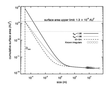
Figure 7: Cumulative surface area plot showing theoretical distributions and the known irregular satellites of Saturn. The black dotted line is the upper limit on the surface area implied by the MIPS observations. The grey dotted line is the less conservative upper limit.

Our predictions in Kennedy & Wyatt (2011) were based on a two phase size distribution, which fit the size distribution of known irregulars. The two phases arise because object strength sets the size distribution slope (O’Brien & Greenberg, 2003), and there are two different strength regimes (e.g. Durda et al., 1998; Benz & Asphaug, 1999; Stewart & Leinhardt, 2009). Above the $\sim$0.1km transition size, objects gaining strength from self-gravity have a shallower slope ($q_{\rm grav}$) than smaller objects, whose strength is derived from material properties (and have a slope $q_{\rm str}$). The slope in the strength regime is generally negative because larger objects are more likely to have a significant flaw (e.g. Benz & Asphaug, 1994). The slope $q_{\rm str}$ is flatter (less negative) for more porous objects (e.g. Housen & Holsapple, 1990, 2011).

While studies generally agree that the strength and gravity regimes exist, the transition size and dependence of strength on size varies between authors. In predicting a level of 320Jy for Saturn’s dust cloud Kennedy & Wyatt (2011), we used a transition size of 0.1km, $q_{\rm str}=1.9$, and $q_{\rm grav}=1.7$.

Figure 7 compares our upper limit with the prediction and two other size distributions. All size distributions end at the assumed minimum grain size $D_{\rm min}=16\mu$m. The black solid line shows our prediction and the dashed line shows the same distribution with a smaller transition size of 5m. The solid grey line shows the same distribution with a slightly flatter size distribution in the strength regime ($q_{\rm str}=1.86$). The observed Saturn irregulars sit at the lower right, illustrating the many orders of magnitude in size between the largest and smallest objects, and why predictions are uncertain. We also include a less conservative (but not unreasonable) limit on surface density, assuming that the Iapetus scans contain no dust and that the dust is made of “real” comet-like grains (see above), which is a factor four lower.

Figure 7 shows that there are several ways the surface area can be lower than the upper limit. The surface area decreases as the minimum grain size $D_{\rm min}$ increases, and for our original prediction would need to be about a factor of ten higher ($\sim$160$\mu$m) to be consistent with the upper limit. Models that explore circumplanetary grain dynamics in this context are therefore needed. If the effective minimum grain size is larger our upper limit becomes less constraining, but if grains are typically smaller it is more constraining.

Alternatively, the transition between the strength and gravity regimes may be smaller than the assumed 0.1km. For the same strength dependence, the transition size needs to be 20 times smaller (5m) to satisfy our upper limit (dashed line). Though there are modest variations, no models predict the transition size to be this small (e.g. Benz & Asphaug, 1999).

A more likely possibility is that the size distribution in the strength regime is flatter, as illustrated by the grey line. The slope of $q_{\rm str}=1.86$ corresponds to a strength dependence of $\propto D^{-0.17}$. For the less conservative limit $q_{\rm str}=1.83$ and the strength dependence is $\propto D^{0.06}$ (i.e. slightly positive). This dependence is flatter than most theoretical models, which lie in the range -0.2 to -0.6 (e.g. Davis & Ryan, 1990; Benz & Asphaug, 1999; Stewart & Leinhardt, 2009). It is significantly flatter than the strength dependence inferred for small asteroids impacting Gaspra and Ida (-1, Greenberg et al., 1994, 1996). A likely reason the strength dependence is flatter than typically predicted or observed is that small irregulars are more porous than asteroids (e.g. Housen & Holsapple, 1990, 2011), and therefore more comet-like (e.g. Greenberg & Hage, 1990; Britt et al., 2002). Strength properties more akin to comets than asteroids are consistent with the proposed scattering and subsequent capture or irregulars from the outer reaches of the Solar System (e.g. Nesvorný et al., 2007). The difference between out upper limit of 45Jy and the prediction of 320Jy may therefore be because the strength of small irregular satellites depends less strongly on their size than we assumed, and the size distribution consequently flatter.

However, the strength prescription could be correct because any additional loss processes (other than collisional evolution) would lead to an overall flatter size distribution. The slightly positive strength dependence for our less conservative upper limit suggests that other loss processes do indeed occur. For Saturn, we estimated that Poynting-Robertson (PR) drag is roughly as important as collisional evolution for removing the smallest grains, and therefore possibly an important loss process that may modify the small end of the size distribution (Kennedy & Wyatt, 2011; Wyatt et al., 2011). For the originally assumed size distribution in Figure 7, the surface area would need to turn over around 160$\mu$m, which is significantly larger than the minimum grain size and therefore unlikely. However, as for the minimum grain size, grain dynamics need to be modelled in detail to study the effect of radiation forces, including other possible effects (e.g. Yarkovsky force).

Observationally, pushing the minimum known sizes of irregular satellites down will better characterise their size distribution over a wider range. However, progress will be difficult. Table 3 in Jewitt & Haghighipour (2007) shows that the faintest known irregulars at Saturn have R magnitudes of 24.5, and the deepest survey for Uranian irregulars had a 50% detection efficiency at $R=26$mag (Sheppard et al., 2005). Such an improvement for Saturnian satellites would push the smallest objects down by a factor of about 4, to about 1km.

Complementary methods that probe smaller sizes are therefore also needed, such as crater counts. While craters have been counted on Saturnian satellites (e.g. Smith et al., 1982; Kirchoff & Schenk, 2010), to back out a size distribution of irregulars is complex. For example, because small and large impactors alter the target’s surface in different ways, the observed crater size distribution does not necessarily reflect the impactor distribution (e.g. Greenberg et al., 1994, 1996; Richardson, 2009). Few studies consider irregular satellites as a source of impactors (see Bottke et al., 2010), probably because most irregulars were only discovered in the last ten years or so and it was only recently proposed that the known irregulars are the tip of an iceberg of collisional fragments (Bottke et al., 2010; Kennedy & Wyatt, 2011). Bottke et al. (2010) make a simple comparison based on their irregular satellite evolution model, but also acknowledge the complications of trying to derive a crater population from a population of irregulars whose size distribution and dynamics evolve as they grind down. Given that the number of irregulars was likely much greater in the past, they may have dominated the impactor population and should be considered when modelling crater counts.

4.2 Future observations

In trying to extract the signal of our proposed dust cloud, we had to consider a number of possible confounding issues. For the ON and OFF scans the Zodiacal contribution could largely be accounted for because the Zodiacal contribution is expected to change little with small changes in elongation. An alternative way to account for ecliptic dust it is to take two observations separated by exactly one year. The first includes the region around the planet, and the second observes the same patch of sky (the planet having moved on in its orbit), and thus has the same line of sight through the ecliptic and the same (extra)galactic background. However, the limiting factor for this study was in fact Spitzer’s PSF. PSF characterisation may be the most important issue for future observations of this type.

Given that instrumental PSFs may be hard to avoid and characterise, an additional way to maximise the chance of a detection is to look for dust around a different planet. The argument for doing so could be due to either a better chance of detection (assuming a similar dust cloud is present), or that the dust cloud is likely to be brighter. For the former case, the giant planets are near their equilibrium temperatures so their spectra are roughly similar to that expected for dust. Therefore, a contrast advantage can be gained by looking at Uranus, which is much fainter and whose dust cloud is expected be of similar surface brightness to that predicted for Saturn (Kennedy & Wyatt, 2011). The question of which planet is more likely to harbour detectable dust is uncertain. Uranus may again be more favourable than Saturn because the dust may be less affected by PR drag (Kennedy & Wyatt, 2011). Dust from irregular satellites at Neptune is probably at a lower level due to the proposed disruption of the population by Triton and/or Nereid (Nesvorný et al., 2003; Ćuk & Gladman, 2005).

While our model considers a large uniform dust cloud, there is also the possibility of smaller scale structures due to individual objects such as the Phoebe ring (Verbiscer et al., 2009). Because they are non-axisymmetric, these structures should be easier to detect. The best candidates appear to be Phoebe, Nereid, and perhaps the Carme collisional family, because their low inclinations relative to our line of sight increase the surface brightness of any associated dust.

5 Summary

We attempted to detect the Saturnian irregular satellite dust cloud proposed to exist by Kennedy & Wyatt (2011) using existing archival Spitzer MIPS observations. A signal was observed, but is consistent with being the PSF due to nearby Saturn, which is likely to be the main issue for future observations. We therefore consider the detection to be an upper limit on the level of dust in the outer reaches of the Saturnian system. In the absence of other loss processes, the upper limit constrains the size distribution of irregulars and therefore their strength properties, which we find to be more akin to comets than asteroids. This conclusion is consistent with their presumed capture from the outer regions of the Solar System.

This work is based in part on observations made with the Spitzer Space Telescope, which is operated by the Jet Propulsion Laboratory, California Institute of Technology under a contract with NASA. This research also made use of Tiny Tim/Spitzer, developed by John Krist for the Spitzer Science Center. The Center is managed by the California Institute of Technology under a contract with NASA. We thank John Krist for his advice on the limitations of the STinyTim PSFs.

References

- Benz & Asphaug (1994) Benz, W. & Asphaug, E. 1994, Icarus, 107, 98 [ADS]
- Benz & Asphaug (1999) —. 1999, Icarus, 142, 5 [ADS]
- Bottke et al. (2010) Bottke, W. F., Nesvorný, D., Vokrouhlický, D., & Morbidelli, A. 2010, AJ, 139, 994 [ADS]
- Britt et al. (2002) Britt, D. T., Yeomans, D., Housen, K., & Consolmagno, G. 2002, Asteroids III, 485 [ADS]
- Burns et al. (1979) Burns, J. A., Lamy, P. L., & Soter, S. 1979, Icarus, 40, 1 [ADS]
- Carruba et al. (2002) Carruba, V., Burns, J. A., Nicholson, P. D., & Gladman, B. J. 2002, Icarus, 158, 434 [ADS]
- Ćuk & Gladman (2005) Ćuk, M. & Gladman, B. J. 2005, ApJ, 626, L113 [ADS]
- Davis & Ryan (1990) Davis, D. R. & Ryan, E. V. 1990, Icarus, 83, 156 [ADS]
- Dohnanyi (1969) Dohnanyi, J. S. 1969, J. Geophys. Res., 74, 2531 [ADS]
- Durda et al. (1998) Durda, D. D., Greenberg, R., & Jedicke, R. 1998, Icarus, 135, 431 [ADS]
- Gladman et al. (2001) Gladman, B., Kavelaars, J. J., Holman, M., Nicholson, P. D., Burns, J. A., Hergenrother, C. W., Petit, J.-M., Marsden, B. G., Jacobson, R., Gray, W., & Grav, T. 2001, Nature, 412, 163 [ADS]
- Greenberg & Hage (1990) Greenberg, J. M. & Hage, J. I. 1990, ApJ, 361, 260 [ADS]
- Greenberg et al. (1996) Greenberg, R., Bottke, W. F., Nolan, M., Geissler, P., Petit, J.-M., Durda, D. D., Asphaug, E., & Head, J. 1996, Icarus, 120, 106 [ADS]
- Greenberg et al. (1994) Greenberg, R., Nolan, M. C., Bottke, Jr., W. F., Kolvoord, R. A., & Veverka, J. 1994, Icarus, 107, 84 [ADS]
- Grogan et al. (2001) Grogan, K., Dermott, S. F., & Durda, D. D. 2001, Icarus, 152, 251 [ADS]
- Housen & Holsapple (1990) Housen, K. R. & Holsapple, K. A. 1990, Icarus, 84, 226 [ADS]
- Housen & Holsapple (2011) —. 2011, Icarus, 211, 856 [ADS]
- Jewitt & Haghighipour (2007) Jewitt, D. & Haghighipour, N. 2007, ARA&A, 45, 261 [ADS]
- Kelsall et al. (1998) Kelsall, T. et al. 1998, ApJ, 508, 44 [ADS]
- Kennedy & Wyatt (2011) Kennedy, G. M. & Wyatt, M. C. 2011, MNRAS, 412, 2137 [ADS]
- Kessler (1981) Kessler, D. J. 1981, Icarus, 48, 39 [ADS]
- Kirchoff & Schenk (2010) Kirchoff, M. R. & Schenk, P. 2010, Icarus, 206, 485 [ADS]
- Li & Greenberg (1998) Li, A. & Greenberg, J. M. 1998, A&A, 331, 291 [ADS]
- Low et al. (1984) Low, F. J. et al. 1984, ApJ, 278, L19 [ADS]
- Nesvorný et al. (2003) Nesvorný, D., Alvarellos, J. L. A., Dones, L., & Levison, H. F. 2003, AJ, 126, 398 [ADS]
- Nesvorný et al. (2007) Nesvorný, D., Vokrouhlický, D., & Morbidelli, A. 2007, AJ, 133, 1962 [ADS]
- O’Brien & Greenberg (2003) O’Brien, D. P. & Greenberg, R. 2003, Icarus, 164, 334 [ADS]
- Richardson (2009) Richardson, J. E. 2009, Icarus, 204, 697 [ADS]
- Rieke et al. (2004) Rieke, G. H. et al. 2004, ApJS, 154, 25 [ADS]
- Sheppard et al. (2005) Sheppard, S. S., Jewitt, D., & Kleyna, J. 2005, AJ, 129, 518 [ADS]
- Smith et al. (1982) Smith, B. A. et al. 1982, Science, 215, 504 [ADS]
- Stewart & Leinhardt (2009) Stewart, S. T. & Leinhardt, Z. M. 2009, ApJ, 691, L133 [ADS]
- Verbiscer et al. (2009) Verbiscer, A. J., Skrutskie, M. F., & Hamilton, D. P. 2009, Nature, 461, 1098 [ADS]
- Wyatt et al. (2011) Wyatt, M. C., Clarke, C. J., & Booth, M. 2011, ArXiv e-prints, (1103.5499) [ADS]
- Wyatt et al. (2007) Wyatt, M. C., Smith, R., Su, K. Y. L., Rieke, G. H., Greaves, J. S., Beichman, C. A., & Bryden, G. 2007, ApJ, 663, 365 [ADS]