Adaptive Finite Element Methods with Inexact Solvers for the Nonlinear Poisson-Boltzmann Equation

1 Introduction

In this article we study adaptive finite element methods (AFEM) with inexact solvers for a class of semilinear elliptic interface problems. We are particularly interested in nonlinear problems with discontinuous diffusion coefficients, such as the nonlinear Poisson-Boltzmann equation and its regularizations. The algorithm we study consists of the standard SOLVE-ESTIMATE-MARK-REFINE procedure common to many adaptive finite element algorithms, but where the SOLVE step involves only a full solve on the coarsest level, and the remaining levels involve only single Newton updates to the previous approximate solution. We summarize a recently developed AFEM convergence theory for inexact solvers appearing in Bank et al. (2011), and present a sequence of numerical experiments that give evidence that the theory does in fact predict the contraction properties of AFEM with inexact solvers. The various routines used are all designed to maintain a linear-time computational complexity.

An outline of the paper is as follows. In Section 2, we give a brief overview of the Poisson-Boltzmann equation. In Section 3, we describe AFEM algorithms, and introduce a variation involving inexact solvers. In Section 4, we give a sequence of numerical experiments that support the theoretical statements on convergence and optimality. Finally, in Section 5 we make some final observations.

2 Regularized Poisson-Boltzmann Equation

We use standard notation for Sobolev spaces. In particular, we denote $\|\cdot\|_{0,G}$ the $L^{2}$ norm on any subset $G\subset\mathbb{R}^{3},$ and denote $\|\cdot\|_{1,2,G}$ the $H^{1}$ norm on $G$.

Let $\Omega:=\Omega_{m}\cup\Gamma\cup\Omega_{s}$ be a bounded Lipschitz domain in $\mathbb{R}^{3}$, which consists of the molecular region $\Omega_{m},$ the solvent region $\Omega_{s}$ and their interface $\Gamma:=\overline{\Omega}_{m}\cap\overline{\Omega}_{s}$ (see Figure 1).

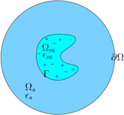
Figure 1: Schematic of a molecular domain.

Our interest in this paper is to solve the following regularized Poisson-Boltzmann equation in the weak form: find $u\in H_{g}^{1}(\Omega):=\{u\in H^{1}(\Omega):u|_{\partial\Omega}=g\}$ such that

$$a(u,v)+(b(u),v)=(f,v)\quad\forall v\in H_{0}^{1}(\Omega),$$ (1)

where $a(u,v)=\int_{\Omega}\epsilon\nabla u\cdot\nabla vdx,$ $(b(u),v)=\int_{\Omega}\kappa^{2}\sinh(u)vdx$. Here we assume that the diffusion coefficient $\epsilon$ is piecewise positive constant $\epsilon|_{\Omega_{m}}=\epsilon_{m}$ and $\epsilon|_{\Omega_{s}}=\epsilon_{s}$. The modified Debye-Hückel parameter $\kappa^{2}$ is also piecewise constant with $\kappa^{2}(x)|_{\Omega_{m}}=0$ and $\kappa^{2}(x)|_{\Omega_{s}}>0$. The equation (1) arises from several regularization schemes (cf. Chen et al. (2007); Chern et al. (2003)) of the nonlinear Poisson-Boltzmann equation:

$$-\nabla\cdot(\epsilon\nabla u)+\kappa^{2}\sinh u=\sum_{i=1}^{N}z_{i}\delta(x_{i}),$$

where the right hand side represents $N$ fixed points with charges $z_{i}$ at positions $x_{i}$, and $\delta$ is the Dirac delta distribution.

It is easy to verify that the bilinear form in (1) satisfies:

$$c_{0}\|u\|_{1,2}^{2}\leq a(u,u),\qquad a(u,v)\leq c_{1}\|u\|_{1,2}\|v\|_{1,2},\qquad\forall u,v\in H_{0}^{1}(\Omega),$$

where $0<c_{0}\leq c_{1}<\infty$ are constants depending only on $\epsilon$. These properties imply the norm on $H_{0}^{1}(\Omega)$ is equivalent to the energy norm $|||\cdot|||\colon H_{0}^{1}(\Omega)\rightarrow\mathbb{R}$,

$$|||u|||^{2}=a(u,u),\qquad c_{0}\|u\|_{1,2}^{2}\leq|||u|||^{2}\leq c_{1}\|u\|_{1,2}^{2}.$$

Let $\mathcal{T}_{h}$ be a shape-regular conforming triangulation of $\Omega$, and let $V_{g}(\mathcal{T}_{h}):=\{v\in H^{1}(\Omega):v|_{\tau}\in\mathbb{P}_{1}(\tau)\;\;\forall\tau\in\mathcal{T}_{h}\}$ be the standard piecewise linear finite element space defined on $\mathcal{T}_{h}$. For simplicity, we assume that the interface $\Gamma$ is resolved by $\mathcal{T}_{h}$. Then the finite element approximation of (1) reads: find $u_{h}\in V_{g}(\mathcal{T}_{h})$ such that

$$a(u_{h},v)+(b(u_{h}),v)=(f,v),\quad\forall v\in V_{0}(\mathcal{T}_{h}).$$ (2)

We close this section with a summary of a priori $L^{\infty}$ bounds for the solution $u$ to (1) and the discrete solution $u_{h}$ to (2), which play a key role in the finite element error analysis of (2) and adaptive algorithms. For interested reader, we refer to Chen et al. (2007); Holst et al. (2009) for details.

Theorem 2.1

There exist $u_{+},u_{-}\in L^{\infty}(\Omega)$ such that the solution $u$ of (1) satisfies the following a priori $L^{\infty}$ bounds:

$$u_{-}\leq u\leq u_{+},\qquad\mbox{ a.e. in }\Omega.$$ (3)

Moreover, if the triangulation $\mathcal{T}_{h}$ satisfies that

$$a(\phi_{i},\phi_{j})\leq-\frac{\sigma}{h^{2}}\sum_{e_{i,j}\subset\tau}|\tau|,\quad\mbox{for some}\quad\sigma>0,$$ (4)

for all the adjacent vertices $i\neq j$ with the basis function $\phi_{i}$ and $\phi_{j},$ then the discrete solution $u_{h}$ of (2) also has the a priori $L^{\infty}$ bound

$$\|u_{h}\|_{L^{\infty}(\Omega)}\leq C,$$ (5)

where $C$ is a constant independent of $h.$

We note that the mesh condition is generally not needed practically, and in fact can also be avoided in analysis for certain nonlinearites Bank et al. (2011).

3 Adaptive FEM with Inexact Solvers

Given a discrete solution $u_{h}\in V_{g}(\mathcal{T}_{h})$, let us define the residual based error indicator $\eta(u_{h},\tau)$:

$$\eta^{2}(u_{h},\tau)=h_{\tau}^{2}\|b(u_{h})-f\|_{0,\tau}^{2}+\sum_{e\subset\partial\tau}h_{e}\|[(\epsilon\nabla u_{h})\cdot n_{e}]\|^{2}_{0,e},$$

where $[(\epsilon\nabla u_{h})\cdot n_{e}]$ denote the jump of the flux across a face $e$ of $\tau.$ For any subset $\mathcal{S}\subset\mathcal{T}_{h},$ we set $\eta^{2}(u_{h},\mathcal{S}):=\sum_{\tau\in\mathcal{S}}\eta^{2}(u_{h},\tau).$ By using the a priori $L^{\infty}$ bounds Theorem  2.1, we can show (cf. Holst et al. (2009)) that the error indicator satisfies:

$$|||u-u_{h}|||^{2}\leq C_{1}\eta^{2}(u_{h},\hat{\mathcal{T}}_{h});$$ (6)

and

$$|\eta(v,\tau)-\eta(w,\tau)|\leq C_{2}|||v-w|||_{\omega_{\tau}},\quad\forall v,w\in V_{g}(\mathcal{T}_{h})$$ (7)

where $\omega_{\tau}=\cup_{\tau^{\prime}\in\mathcal{T}_{h},\bar{\tau}^{\prime}\cap\bar{\tau}\neq\emptyset}\tau^{\prime}$ and $|||v|||_{\omega_{\tau}}^{2}=\int_{\omega_{\tau}}\epsilon|\nabla v|^{2}dx$.

Given an initial triangulation $\mathcal{T}_{0}$, the standard adaptive finite element method (AFEM) generates a sequence $\left[u_{k},\mathcal{T}_{k},\{\eta(u_{k},\tau)\}_{\tau\in\mathcal{T}_{k}}\right]$ based on the iteration of the form:

$$\hbox{$\textsf{SOLVE}$}\rightarrow\hbox{$\textsf{ESTIMATE}$}\rightarrow\hbox{$\textsf{MARK}$}\rightarrow\hbox{$\textsf{REFINE}$}.$$

Here the SOLVE subroutine is usually assumed to be exact, namely $u_{k}$ is the exact solution to the nonlinear equation (2); the ESTIMATE routine computes the element-wise residual indicator $\eta(u_{k},\tau)$; the MARK routine uses standard Dörfler marking (cf. Dörfler (1996)) where $\mathcal{M}_{k}\subset\mathcal{T}_{k}$ is chosen so that

$$\eta(u_{k},\mathcal{M}_{k})\geq\theta\eta(u_{k},\mathcal{T}_{k})$$

for some parameter $\theta\in(0,1];$ finally, the routine REFINE subdivide the marked elements and possibly some neighboring elements in certain way such that the new triangulation preserves shape-regularity and conformity.

During last decade, a lot of theoretical work has been done to show the convergence of the AFEM with exact solver (see Nochetto et al. (2009) and the references cited therein for linear PDE case, and Holst et al. (2010) for nonlinear PDE case). To the best of the authors knowledge, there are only a couple of convergence results of AFEM for symmetric linear elliptic equations (cf. Stevenson (2007); Arioli et al. (2009)) which take the numerical error into account. To distinct with the exact solver case, we use $\hat{u}_{k}$ and $\hat{\mathcal{T}}_{k}$ to denote the numerical approximation to (2) and the triangulation obtained from the adaptive refinement using the inexact solutions.

Due to the page limitation, we only state the main convergence result of the AFEM with inexact solver for solving (1) below. More detailed analysis and extension are reported in Bank et al. (2011).

Theorem 3.1

Let $\{\hat{\mathcal{T}}_{k},\hat{u}_{k}\}_{k\geq 0}$ be the sequence of meshes and approximate solutions computed by the AFEM algorithm. Let $u$ denote the exact solution and $u_{k}$ denote the exact discrete solutions on the meshes $\hat{\mathcal{T}}_{k}$. Then, there exist constants $\mu>0$, $\nu\in(0,1)$, $\gamma>0$, and $\alpha\in(0,1)$ such that if the inexact solutions satisfy

$$\mu|||u_{k}-\hat{u}_{k}|||^{2}+|||u_{k+1}-\hat{u}_{k+1}|||^{2}\leq\nu\eta^{2}(\hat{u}_{k},\hat{\mathcal{T}}_{k})$$ (8)

then

$$|||u-u_{k+1}|||^{2}+\gamma\eta^{2}(\hat{u}_{k+1},\hat{\mathcal{T}}_{k+1})\leq\alpha^{2}(|||u-u_{k}|||^{2}+\gamma\eta^{2}(\hat{u}_{k},\hat{\mathcal{T}}_{k})).$$ (9)

Consequently, $\lim_{k\to\infty}u_{k}=\lim_{k\to\infty}\hat{u}_{k}=u.$

The proof of this theorem is based on the upper bound (6) of the exact solution, the Lipschitz property (7) of the error indicator, Dörfler marking, and the following quasi-orthogonality between the exact solutions:

$$|||u-u_{k+1}|||^{2}\leq\Lambda|||u-u_{k}|||^{2}-|||u_{k+1}-u_{k}|||^{2}$$ (10)

where $\Lambda$ can be made close to 1 by refinement. For a proof of the inequality (10), see for example Holst et al. (2009).

To achieve the optimal computational complexity, we should avoid solving the nonlinear system (2) as much as we could. The two-grid algorithm Xu (1996) shows that a nonlinear solver on a coarse grid combined with a Newton update on the fine grid still yield quasi-optimal approximation. Motivated by this idea, we propose the following AFEM algorithm with inexact solver, which contains only one nonlinear solver on the coarsest grid, and Newton updates on each follow-up steps:

Algorithm 1 : $\left[\hat{u}_{k},\hat{\mathcal{T}}_{k},\{\eta(\hat{u}_{k},\tau)\}_{\tau\in\hat{\mathcal{T}_{k}}}\right]:=$ Inexact_AFEM$(\mathcal{T}_{0},\theta)$

1   $\hat{u}_{0}=u_{0}:=$ NSOLVE$(\mathcal{T}_{0})$     %Nonlinear solver on initial triangulation

2   for $k:=0,1,\cdots$ do

3        $\{\eta(\hat{u}_{k},\tau)\}_{\tau\in\hat{\mathcal{T}_{k}}}:=\textsf{ESTIMATE}(\hat{u}_{k},\hat{\mathcal{T}}_{k})$

4        $\mathcal{M}_{k}:=\textsf{MARK}(\{\eta(\hat{u}_{k},\tau)\}_{\tau\in\hat{\mathcal{T}_{k}}},\hat{\mathcal{T}}_{k},\theta)$

5        $\hat{\mathcal{T}}_{k+1}:=\textsf{REFINE}(\hat{\mathcal{T}}_{k},\mathcal{M}_{k})$

6        $\hat{u}_{k+1}:=\textsf{UPDATE}(\hat{u}_{k},\hat{\mathcal{T}}_{k+1})$    %One-step Newton update

7   end

In Algorithm 1, the NSOLVE routine is used only on the coarsest mesh and is implemented using Newton’s method run to certain convergence tolerance. For the rest of the solutions, a single step of Newton’s method is used to update the previous approximation. That is, UPDATE computes $\hat{u}_{k+1}$ such that

$$a(\hat{u}_{k+1}-\hat{u}_{k},\phi)+(b^{\prime}(\hat{u}_{k})(\hat{u}_{k+1}-\hat{u}_{k}),\phi)=0$$ (11)

for every $\phi\in V(\hat{\mathcal{T}}_{k+1})$. We remark that since (11) is only a linear problem, we could use the local multilevel method to solve it in (near) optimal complexity (cf. Chen et al. (2010)). Therefore, the overall computational complexity of the Algorithm 1 is nearly optimal.

We should point out that it is not obvioius how to enforce the required approximation property (8) that $\hat{u}_{k}$ must satisfy for the theorem. This is examined in more detail in Bank et al. (2011). However, numerical evidence in the following section shows Algorithm 1 is an efficient algorithm, and the results matches the ones from AFEM with exact solver.

4 Numerical Experiments

In this section we present some numerical experiments to illustrate the result in Theorem 3.1, implemented with FETK. The software utilizes the standard piecewise-linear finite element space for discretizing (1). Algorithm 1 is implemented with care taken to guarantee that each of the steps runs in linear time relative to the number of vertices in the mesh. The linear solver used is Conjugate Gradients preconditioned by diagonal scaling. The estimator is computed using a high-order quadrature rule, and, as mentioned above, the marking strategy is Dörfler marking where the estimated error have been binned to maintain linear complexity while still marking the elements with the largest error. Finally, the refinement is longest edge bisection, with refinement outside of the marked set to maintain conformity of the mesh.

We present three sets of results in order to explore the effects of the inexact solver in multiple contexts. For all problems, we present a convergence plot using both inexact and exact solvers (including a reference line of order $N^{-\frac{1}{3}}$) as well as a representative cut-away of a mesh with around 30,000 vertices. The exact discrete solution is computed using the standard AFEM algorithm where the solution on each mesh is computed by allowing Newton’s method to continue running to convergence to within a tolerance of $10^{-8}$. This modifies not only the solution on a given mesh, but also the sequence of meshes generated, since the algorithm may mark different simplices. However, in all cases, convergence is identical to high precision and meshes place the unknowns as expected.

The first result uses constant coefficients across the entire domain $\Omega=[0,1]^{3}$ and we choose a right hand side so that the derivative of the exact solution is large near the origin. The boundary conditions chosen for this problem are homoegenous Dirichlet boundary conditions. Specifically, the exact solution is given by $u=u_{1}u_{2}$ where

$$u_{1}=\sin(\pi x)\sin(\pi y)\sin(\pi z)$$

is chosen to satisfy the boundary condition and

$$u_{2}=(x^{2}+y^{2}+x^{2}+10^{-4})^{-1.5}.$$

The results can be seen in Figure 2.

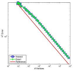
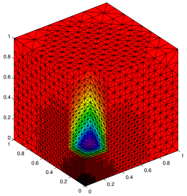
Figure 2: Convergence plot and mesh cut-away for the corner singularity problem.

The second result uses the domain $\Omega=[-1,1]^{3}$ and $\Omega_{m}=\left[-\frac{1}{4},\frac{1}{4}\right]$ with constants $\epsilon_{s}=80,\epsilon_{m}=2,\kappa_{s}=1,$ and $\kappa_{m}=0$. Homogeneous Neumann conditions are chosen for the boundary and the right hand side is simplified to a constant. Because an exact solution is unavailable for this (and the following) problem, the error is computed by comparing to a discrete solution on a mesh with around 10 times the number of vertices as the finest mesh used in the adaptive algorithm. Figure 3 shows the results for this problem. As can be seen the refinement favors the interface and the inexact and exact solvers perform as expected.

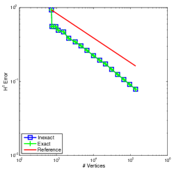
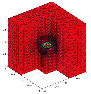
Figure 3: Convergence plot and mesh cut-away for the Poisson-Boltzmann problem.

The final result is chosen to test the robustness of the inexact method to large coefficient jumps. The domain and boundary conditions are the same as the previous example, but the constants chosen as are $\epsilon_{s}=1000,\epsilon_{m}=10,\kappa_{s}=1,$ and $\kappa_{m}=0$. The results can be seen in Figure 4, and they show a scenario very similar to the previous example, with the refinement restricted even further to the interface.

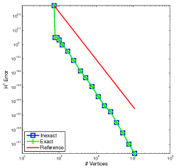
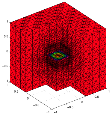
Figure 4: Convergence plot and mesh cut-away for the exaggerated-jump Poisson-Boltzmann problem.

5 Conclusion

In this article we have studied AFEM with inexact solvers for a class of semilinear elliptic interface problems with discontinuous diffusion coefficients, with emphasis on the nonlinear Poisson-Boltzmann equation. The algorithm we studied consisted of the standard SOLVE-ESTIMATE-MARK-REFINE procedure common to many adaptive finite element algorithms, but where the SOLVE step involves only a full solve on the coarsest level, and the remaining levels involve only single Newton updates to the previous approximate solution. The various routines used are all designed to maintain a linear-time computational complexity. Our numerical results indicate that the recently developed AFEM convergence theory for inexact solvers in Bank et al. (2011) does predict the actual behavior of the methods.

References

- Arioli et al. [2009] M. Arioli, E.H. Georgoulis, and D. Loghin. Convergence of inexact adaptive finite element solvers for elliptic problems. Technical Report RAL-TR-2009-021, Science and Technology Facilities Council, October 2009.
- Bank et al. [2011] R. Bank, M. Holst, R. Szypowski, and Y. Zhu. Convergence of AFEM for semilinear problems with inexact solvers. Preprint, 2011.
- Chen et al. [2010] L. Chen, M. Holst, J. Xu, and Y. Zhu. Local Multilevel Preconditioners for Elliptic Equations with Jump Coefficients on Bisection Grids. Arxiv preprint arXiv:1006.3277, 2010.
- Chen et al. [2007] Long Chen, Michael Holst, and Jinchao Xu. The finite element approximation of the nonlinear Poisson-Boltzmann equation. SIAM Journal on Numerical Analysis, 45(6):2298–2320, 2007.
- Chern et al. [2003] I-Liang Chern, Jian-Guo Liu, and Wei-Cheng Wan. Accurate evaluation of electrostatics for macromolecules in solution. Methods and Applications of Analysis, 10:309–328, 2003.
- Dörfler [1996] W. Dörfler. A convergent adaptive algorithm for Poisson’s equation. SIAM Journal on Numerical Analysis, 33:1106–1124, 1996.
- Holst et al. [2009] M. Holst, J.A. McCammon, Z. Yu, Y.C. Zhou, and Y. Zhu. Adaptive Finite Element Modeling Techniques for the Poisson-Boltzmann Equation. Accepted for publication in Communications in Computational Physics, 2009.
- Holst et al. [2010] M. Holst, G. Tsogtgerel, and Y. Zhu. Local Convergence of Adaptive Methods for Nonlinear Partial Differential Equations. arXiv, (1001.1382v1), 2010.
- Nochetto et al. [2009] R.H. Nochetto, K.G. Siebert, and A. Veeser. Theory of adaptive finite element methods: An introduction. In R.A. DeVore and A. Kunoth, editors, Multiscale, Nonlinear and Adaptive Approximation, pages 409–542. Springer, 2009.
- Stevenson [2007] Rob Stevenson. Optimality of a standard adaptive finite element method. Found. Comput. Math., 7(2):245–269, 2007.
- Xu [1996] Jinchao Xu. Two-grid discretization techniques for linear and nonlinear PDEs. SIAM Journal on Numerical Analysis, 33(5):1759–1777, 1996.