Pseudospectral Calculation of Helium Wave Functions, Expectation Values, and Oscillator Strength

Abstract

The pseudospectral method is a powerful tool for finding highly precise solutions of Schrödinger’s equation for few-electron problems. Previously we developed the method to calculate fully correlated S-state wave functions for two-electron atoms Grabowski and Chernoff (2010). Here we extend the method’s scope to wave functions with non-zero angular momentum and test it on several challenging problems. One group of tests involves the determination of the nonrelativistic electric dipole oscillator strength for the helium $1^{1}$S $\to 2^{1}$P transition. The result achieved, $0.27616499(27)$, is comparable to the best in the literature. The formally equivalent length, velocity, and acceleration expressions for the oscillator strength all yield roughly the same accuracy because the numerical method constrains the wave function errors in a local fashion.

Another group of test applications is comprised of well-studied leading order finite nuclear mass and relativistic corrections for the helium ground state. A straightforward computation reaches near state-of-the-art accuracy without requiring the implementation of any special-purpose numerics.

All the relevant quantities tested in this paper – energy eigenvalues, S-state expectation values and bound-bound dipole transitions for S and P states – converge exponentially with increasing resolution and do so at roughly the same rate. Each individual calculation samples and weights the configuration space wave function uniquely but all behave in a qualitatively similar manner. Quantum mechanical matrix elements are directly and reliably calculable with pseudospectral methods.

The technical discussion includes a prescription for choosing coordinates and subdomains to achieve exponential convergence when two-particle Coulomb singularities are present. The prescription does not account for the wave function’s non-analytic behavior near the three-particle coalescence which should eventually hinder the rate of the convergence. Nonetheless the effect is small in the sense that ignoring the higher-order coalescence does not appear to affect adversely the accuracy of any of the quantities reported nor the rate at which errors diminish.

I Introduction

The aim of this work is to test and validate the pseudospectral method as a high-precision few-electron problem solver, capable of calculating state-of-the-art precision matrix elements. The helium atom has been studied extensively since the birth of quantum mechanics and so makes a great testbed problem. High-precision work continues to this day to infer fundamental constants such as the fine structure constant (see Ref. Pachucki and Yerokhin (2011a)) and the electron-proton mass ratio (see Ref. Korobov and Zhong (2009a)) by comparing theoretical and experimental measurements. Any theoretical method which may be applied to a variety of problems (e.g. high-precision relativistic corrections, different interaction potentials, excitation levels, symmetries, etc.) without tinkering with or modifying the basis and which has direct, rigorous control of local errors serves as a complementary approach to the variational method.

Methods based on the variational principle, in which the expectation value of the Hamiltonian is minimized with respect to the parameters of a trial wave function, are the most widely used techniques for finding an approximate representation of the ground state. The calculated energy is an upper bound to the exact energy. If one regards the best approximate wave function as first order accurate then the variationally determined energy eigenvalue is second order accurate. Small errors in the energy eigenvalue of a given state imply that the square of the wave function is accurate in the energy-weighted norm but it does not follow that local wave function errors are also small. In practical terms, while the variational approach excels at determining energy eigenvalues it does not generally achieve comparable accuracy in quantum mechanical matrix elements formed from the wave function.

To achieve ever-more accurate energies and/or wave functions in the variational approach one must select a sequence of trial functions capable of representing the exact solution ever-more closely. The choice of a good sequence entails more than a little art and intuition, especially for a nonstandard problem where one may have only a vague idea what the ultimate limit looks like. A sequence of increasing basis size $n$ may be said to converge exponentially if the errors are proportional to $e^{-an}$ for some positive constant $a$. This most favorable outcome is achieved only if the basis can reproduce the analytic properties of the exact wave function. Otherwise, convergence is expected to be algebraic, i.e. $\propto n^{-2}$, or worse.

Recently, we applied pseudospectral methods to solve the nonrelativistic Schrödinger equation for helium and the negatively charged hydrogen ion with zero total angular momentum Grabowski and Chernoff (2010). We found exponentially fast convergence of most quantities of interest including the energy eigenvalues, local energy errors (e.g. $(\hat{H}\Psi)/\Psi-E$ as a function of position) and Cauchy wave function differences. Only the error in the logarithmic derivative near the triple coalescence point had discernibly slower convergence, presumably due to the logarithmic contributions located there Bartlett (1937); Fock (1954, 1958). The key virtues of the pseudospectral approach were: no explicit assumptions had to be made about the asymptotic behavior of the wave function near cusps or at large distances, the Schrödinger equation was satisfied at all grid points, local errors decreased exponentially fast with increasing resolution, and no fine tuning was required.

In this article, we extend our previous work to higher angular momentum calculations and utilize the results to evaluate matrix elements for combinations of states. To be systematic, we consider two sorts of matrix elements: the dipole absorption oscillator strength (between S and P states) and first-order mass polarization and $\alpha^{2}$ relativistic corrections to the nonrelativistic finite-nuclear-mass Hamiltonian (for the S ground state). All have been the subject of extensive investigation. Our main focus is on testing the pseudospectral method’s capabilities by recalculating these quantities and comparing to effectively “exact” published results.

The plan of the paper is as follows. The first four sections are largely background: §II provides an overview of the pseudospectral method; §III describes the two-electron atom, the Bhatia-Temkin coordinate system, the expansion of the wave function in terms of eigenstates and the form of the Hamiltonian; §IV defines length, velocity and acceleration forms for the oscillator strength and related sum rules. The next two sections detail our pseudospectral method of calculation and those readers primarily interested in seeing the results may skip to §VII. §V gives a prescription for how to choose coordinates and subdomains for second order partial differential equations and outlines the special coordinate choices needed to deal with the Coulomb singularities. §VI schematically describes how overlapping and touching grids are coupled together and how symmetry is imposed on the wave function. §VII presents the first group of test results on energies and oscillator strengths. The convergence rate of all quantities is studied in detail. §VIII and §IX review lowest-order corrections to the Hamiltonian due to finite nuclear mass and finite $\alpha$. §X presents the second group of test results for individual corrections to the ground state of He. §XI summarizes the capabilities and promise of the pseudospectral method.

The appendix is divided into four parts. Appendix A gives the explicit form of the Hamiltonian operator used in this article. Appendix B describes how the Hamiltonian matrix problem is solved, gives details of the eigenvalue solver method, and how quantum mechanical matrix elements are calculated once the wave function is determined. Appendix C gives the particular equations for calculating the oscillator strengths and expectation values. Appendix D discusses and tabulates past work done to calculate oscillator strengths.

II Review of pseudospectral methods

Pseudospectral methods have proven success in solving systems of partial differential equations germane to the physics in a wide variety of fields including fluid dynamics Canuto et al. (1988), general relativity Kidder and Finn (2000); Pfeiffer et al. (2003), and quantum chemistry Friesner (1985, 1986, 1987); Ringnalda et al. (1990); Greeley et al. (1994); Murphy et al. (1995, 2000); Ko et al. (2008); Heyl and Thirumalai (2010). Some problems in one-electron quantum mechanics Borisov (2001); Boyd et al. (2003) have been treated but only recently has the method been applied to the case of fully correlated, multi-electron atoms Grabowski and Chernoff (2010). Pseudospectral methods are discussed in some generality in Refs. Boyd (2000); Fornberg (1996a); Orszag (1980); Pfeiffer et al. (2003); Press et al. (2007); Grabowski and Chernoff (2010).

The pseudospectral method is a grid-based finite difference method in which the order of the finite differencing is equal to the resolution of the grid in each direction. As the grid size increases it becomes more accurate than any fixed-order finite difference method. If a solution is smooth over an entire domain (or smooth in each subdomain) the pseudospectral method converges exponentially fast to the solution. A spectral basis expansion and a pseudospectral expansion of the same order are nearly equivalent having differences that are exponentially small.

The grid points in the pseudospectral method are located at the roots of Jacobi polynomials or their antinodes plus endpoints. They are clustered more closely near the boundary of a domain than in its center. Such an arrangement is essential for the method to limit numerical oscillations sourced by singularities beyond the numerical domain Fornberg (1996b). These singularities typically occur in the analytic continuation of solutions to non-physical regimes and/or from the extension of coordinates beyond the patches on which they are defined to be smooth and differentiable. The grid point arrangement facilitates a convergent representation of a function and its derivative across the domain of interest. The interpolated function is more uniformly accurate than is possible using an equal number of equidistant points, as is typical for finite difference methods.

Consider the problem of the pseudospectral representation of an operator like the Hamiltonian. The full domain is multi-dimensional but focus for the moment on a single dimension of the domain. Let $\{\mathbf{{\rm X}}^{k}\}_{k=1,2,\ldots N}$ be the roots of an $N$th order Jacobi polynomial enumerated by $k$. Let $\mathbf{{\rm X}}$ stand for an arbitrary coordinate value in the dimension of interest. Define the one dimensional cardinal functions

$$C_{j}[{\rm X}]=\prod_{\begin{subarray}{c}k=1\\ k\neq j\end{subarray}}^{N}\frac{{\rm X}-{\rm X}^{k}}{{\rm X}^{j}-{\rm X}^{k}}$$ (1)

and note the relation

$$C_{j}[{\rm X}^{k}]=\delta_{j}^{k}$$ (2)

follows. Now let the $n_{d}$-dimensional grid be the tensor product of the individual, one dimensional coordinate grids labeled by $X_{(i)}$ for $i=1$ to $n_{d}$. The corresponding cardinal functions are

$${\cal C}_{J}[\mathbf{{\rm X}}]=\prod_{i=1}^{n_{d}}C_{j_{(i)}}[{\rm X}_{(i)}],$$ (3)

where subscript $J=\{j_{(1)},j_{(2)},\ldots,j_{(n_{d})}\}$ and unadorned $\mathbf{{\rm X}}=\{{\rm X}_{(1)},{\rm X}_{(2)},\ldots,{\rm X}_{(n_{d})}\}$. These multi-dimensional Cardinal functions have the property

$${\cal C}_{J}[\mathbf{{\rm X}}^{K}]=\delta_{J}^{K},$$ (4)

where the grid point $\mathbf{{\rm X}}^{K}=\{{\rm X}_{(1)}^{k_{1}},{\rm X}_{(2)}^{k_{2}},\ldots,{\rm X}_{(n_{d})}^{k_{n_{d}}}\}$. They form a basis in the sense that a general function $f$ can be written

$$f[\mathbf{{\rm X}}]=\sum_{J}f[\mathbf{{\rm X}}^{J}]{\cal C}_{J}[\mathbf{{\rm X}}],$$ (5)

where $f[{{\rm X}}^{J}]$ is a pseudospectral coefficient (“pseudo” because it is more easily identified as the function value at the grid point).

Let the position $\mathbf{{\rm X}}^{K}$ and cardinal ${\cal C}_{J}$ eigenstates be denoted $|\mathbf{{\rm X}}^{K}\rangle$ and $|\mathbf{\cal C}_{J}\rangle$, respectively. The pseudospectral approximation to the Hamiltonian is

$$\hat{H}_{PS}=\sum_{JK}|\mathbf{{\rm X}}^{K}\rangle\langle\mathbf{{\rm X}}^{K}|\hat{H}|{\cal C}_{J}\rangle\langle{\cal C}_{J}|,$$ (6)

where $\hat{H}$ is the full Hamiltonian operator. In practice, the matrix $\langle\mathbf{{\rm X}}^{K}|\hat{H}_{PS}|{\cal C}_{J}\rangle$ is truncated and then diagonalized to find the energy eigenvalues. When the wave function is represented by a pseudospectral expansion the eigenvectors are simply the function values at the grid points. In a spectral representation, by contrast, the eigenvectors are sums of basis functions. It is often more convenient and efficient to work with the local wave function values directly. On the other hand, the truncated operator $\hat{H}_{PS}$ need not be Hermitian at finite resolution, a property that may introduce non-physical effects, e.g. $\langle\mathbf{{\rm X}}^{K}|\hat{H}_{PS}|{\cal C}_{J}\rangle$ may possess complex eigenvalues. Generally, unphysical artifacts quickly reveal themselves as resolution increases. An examination of the eigenvalue spectrum shows that the complex eigenvalues do not converge, permitting separation of physical and unphysical values.

III The nonrelativistic two-electron atom

Two-electron atoms are three-particle systems requiring nine spatial coordinates for a full description. In the absence of external forces, three coordinates are eliminated by taking out the center-of-mass motion. In the infinite-nuclear-mass and nonrelativistic approximations the Hamiltonian is

$$\hat{H}_{0}=-\frac{1}{2}(p_{1}^{2}+p_{2}^{2})+\hat{V},$$ (7)

where $\mathbf{p}_{1,2}$ are the momenta of the two electrons and the potential is

$$\hat{V}=-\frac{Z}{r_{1}}-\frac{Z}{r_{2}}+\frac{1}{r_{12}},$$ (8)

where $Z$ is the nuclear charge, and $r_{1}$, $r_{2}$, and $r_{12}$ are the magnitudes of the vectors pointing from the nucleus to each electron and of the vector pointing from one electron to the other, respectively. Here and throughout this article, atomic units are used. For the infinite-nuclear-mass approximation, the electron mass is set to unity; for a finite nuclear mass, the reduced mass of the electron and nucleus is set to one. The fully correlated wave functions are six-dimensional at this stage.

A further reduction is straightforward for S states. Hylleraas Hylleraas (1929) proposed the ansatz that the wave function be written in terms of three internal coordinates. Typical choices for these coordinates are $r_{1}$, $r_{2}$, and $r_{12}$. Alternatively, $r_{12}$ may be replaced by $\theta_{12}$, the angle between the two electrons. The S state is independent of the remaining three coordinates that describe the orientation of the triangle with vertices at the two electrons and nucleus.

The situation for states of general angular momentum is more complicated. Bhatia and Temkin Bhatia and Temkin (1964) introduced a particular set of Euler angles $\{\Theta,\Phi,\Psi\}$ to describe the triangle’s orientation. They defined a set of generalized spherical harmonics $D_{\kappa lm}^{\nu}$ which are eigenstates of operators for the total angular momentum, its $z$ component, total parity ($\{\mathbf{r}_{1},\mathbf{r}_{2}\}\to\{-\mathbf{r}_{1},-\mathbf{r}_{2}\}$), and exchange ($\mathbf{r}_{1}\leftrightarrow\mathbf{r}_{2}$):

$$\hat{L}^{2}D_{\kappa lm}^{\nu} = l(l+1)D_{\kappa lm}^{\nu}$$ (9)

$$\hat{L}_{z}D_{\kappa lm}^{\nu} = mD_{\kappa lm}^{\nu}$$ (10)

$$\hat{\Pi}D_{\kappa lm}^{\nu} = (-1)^{\kappa}D_{\kappa lm}^{\nu}$$ (11)

$$\hat{{\cal E}}_{12}D_{\kappa lm}^{\nu} = (-1)^{l+\kappa+\nu}D_{\kappa lm}^{\nu}.$$ (12)

The superscript $\nu$ takes on values $\nu=0$ and $1$ while the integer subscript $\kappa$ obeys $0\leq\kappa\leq l$. The quantum number $\kappa$ is the absolute value of an angular momentum-like quantum number about the body-fixed axis of rotation. Even/odd $\kappa$ determines the parity eigenvalue while the combination $l+\kappa+\nu$ determines the exchange eigenvalue. This basis is especially useful since each of the four operators above commutes with the atomic Hamiltonian, $\hat{H}_{0}$. The spatial eigenfunction $\psi_{klms}[\mathbf{r}_{1},\mathbf{r}_{2}]$ for total spin $s$, total angular momentum $l$, $z$-component of angular momentum $m$, and parity $k=\pm 1$ satisfies

$$\hat{L}^{2}\psi_{klms}[\mathbf{r}_{1},\mathbf{r}_{2}] = l(l+1)\psi_{klms}[\mathbf{r}_{1},\mathbf{r}_{2}]$$ (13)

$$\hat{L}_{z}\psi_{klms}[\mathbf{r}_{1},\mathbf{r}_{2}] = m\psi_{klms}[\mathbf{r}_{1},\mathbf{r}_{2}]$$ (14)

$$\hat{\Pi}\psi_{klms}[\mathbf{r}_{1},\mathbf{r}_{2}] = k\psi_{klms}[\mathbf{r}_{1},\mathbf{r}_{2}]$$ (15)

$$\hat{{\cal E}}_{12}\psi_{klms}[\mathbf{r}_{1},\mathbf{r}_{2}] = (-1)^{s}\psi_{klms}[\mathbf{r}_{1},\mathbf{r}_{2}].$$ (16)

Equations 9-16 imply

$$\psi_{klms}[\mathbf{r_{1}},\mathbf{r_{2}}]=\sum_{\nu=0}^{1}\sideset{}{{}^{\prime}}{\sum}_{\kappa=\nu}^{l}g_{\kappa ls}^{\nu}[r_{1},r_{2},\theta_{12}]D_{\kappa lm}^{\nu}[\Theta,\Phi,\Psi],$$ (17)

where the prime on the sum means that $\kappa$ is restricted to even ($k=1$) or odd ($k=-1$) numbers if parity is even or odd, respectively, and $g_{\kappa ls}^{\nu}$ is a real function of the internal coordinates. The convenience of the Bhatia and Temkin Bhatia and Temkin (1964) coordinate choice is most evident in how one imposes total antisymmetry of the wave function. The spin singlet (triplet) must have a symmetric (antisymmetric) spatial wave function. The properties of the $D_{\kappa lm}^{\nu}$ functions reduce this requirement to

$$\hat{{\cal E}}_{12}g_{\kappa ls}^{\nu}=(-1)^{\nu+\kappa+l+s}g_{\kappa ls}^{\nu}.$$ (18)

The total antisymmetry of a wave function with given $k$, $l$, $m$ and $s$ follows by imposing the above requirement under $r_{1}\leftrightarrow r_{2}$ on each radial function for each $\nu$ and $\kappa$. Note that $(-1)^{\kappa+l+s}$ is fixed directly by the wave function’s $k$, $l$ and $s$. The same requirement applies to both singlet and triplet states up to the difference in the value of $s$.

The full six-dimensional Schrödinger equation for given $l$, $s$, even/odd parity, and any $m$ yields $l$ or $l+1$ (depending on these quantum numbers) coupled three-dimensional equations for $g_{\kappa ls}^{\gamma}$. The indices for $g$ satisfy $\gamma$ = $0$ or $1$ and $0\leq\kappa\leq l$ with even or odd $\kappa$ for even or odd parity. The equations are

$$0=(\hat{H}_{S}-E)g_{\kappa ls}^{\gamma}+\sum_{\nu=0}^{1}\sum_{n=-1}^{1}\hat{H}_{\nu\kappa n}^{\gamma}g_{\kappa+2n,l,s}^{\nu},$$ (19)

where $\hat{H}_{S}$ is the part of the Hamiltonian operator that survives for S states. The summation enumerates couplings with $\gamma\neq\nu$ and/or different $\kappa$ as well as terms that are intrinsic to non-S-states.

Appendix A gives the explicit forms of the operators $\hat{H}_{S}$ and $\hat{H}_{\nu\kappa n}^{\gamma}$.

IV Review of the oscillator strength and dipole radiative transitions

The oscillator strength quantifies the coupling between two eigenstates of $\hat{H}_{0}$ on account of interactions with a perturbing electromagnetic field. It is fundamental for interpreting spectra, including the strength and width of atomic transitions and the lifetimes of atomic states. Sites generating spectra of interest are ubiquitous. They include earth-based laboratories, photospheres of the Sun and distant stars, and the near vacuum between the stars where traces of interstellar matter radiate. The specific applications of the oscillator strength are correspondingly diverse. For example, in laboratories the technique of laser spectroscopy is used to measure energy splittings and frequency-dependent photoabsorption cross sections of highly excited states. Knowledge of the transition probability matrices is needed to interpret which states have been directly and indirectly generated. The transitions are driven by collisional and radiative processes, the latter given in terms of oscillator strengths. In an astrophysical context, on the other hand, observations of stellar emission require oscillator strengths for inferring chemical abundances from absorption or emission of radiation Smith (1973); Biémont and Grevesse (1977). Oscillator strengths have widespread utility.

The practical difficulty in calculating the oscillator strength value is the accurate representation of the initial and final wave functions. Almost from the very beginning of the development of quantum mechanics helium, having but two electrons, has served as a testing ground for new theoretical approaches. Appendix D presents a brief, schematic description of the rich history of such improvements in the service of oscillator strength calculations.

Following Baym Baym (1969) and Bethe and Salpeter Bethe and Salpeter (1957), the nonrelativistic Hamiltonian of a two-electron atom in the presence of an electromagnetic field (infinite-nuclear-mass approximation) is

$$\hat{H}_{EM}=\hat{H}_{0}+\hat{H}_{\textrm{int}},$$ (20)

where $\hat{H}_{0}$ is the Hamiltonian for the isolated atom (Eq. 7) and $\hat{H}_{\textrm{int}}$ describes the interaction of the atom with radiation,

$$\hat{H}_{\textrm{int}}=\sum_{i}\left(-\frac{\mathbf{p}_{i}\cdot\mathbf{A}_{i}+\mathbf{A}_{i}\cdot\mathbf{p}_{i}}{2c}-\frac{A_{i}^{2}}{2c^{2}}+\varphi_{i}\right),$$ (21)

where $\mathbf{A}_{i}$ and $\varphi_{i}$ are the vector and scalar potential, respectively, at the location of the $i$th electron (excluding the atomic Coulomb interactions included in $V$), and $c$ is the speed of light. If the photon number density is small then the second term, corresponding to two-photon processes, is much smaller than the first and if one adopts the transverse gauge then the third term is zero. With these assumptions the non-zero terms are the ones linear in the vector potential.

Only electric dipole-mediated transitions and the associated $f$’s are considered in this article. The length, velocity and acceleration forms for the oscillator strength Hibbert (1975) are

$$f_{ij}^{l} = \frac{2}{3}(E_{j}-E_{i})|\langle j|\mathbf{R}|i\rangle|^{2}$$ (22)

$$f_{ij}^{v} = \frac{2}{3}\frac{1}{E_{j}-E_{i}}|\langle j|\mathbf{P}|i\rangle|^{2}$$ (23)

$$f_{ij}^{a} = \frac{2}{3}\frac{1}{(E_{j}-E_{i})^{3}}\left|\left\langle j\left|\mathbf{A}\right|i\right\rangle\right|^{2}.$$ (24)

Here $E_{i}$ and $E_{j}$ are the energies of the initial and final states. The two-particle operators are

$$\mathbf{R} = \mathbf{r_{1}}+\mathbf{r_{2}}$$ (25)

$$\mathbf{P} = \mathbf{p_{1}}+\mathbf{p_{2}}$$ (26)

$$\mathbf{A} = -\frac{Z\mathbf{r_{1}}}{r_{1}^{3}}-\frac{Z\mathbf{r_{2}}}{r_{2}^{3}},$$ (27)

i.e. the position, momentum and acceleration electron operators. Appendix C presents explicit expressions for $f$ used in the calculations.

If the wave functions, energies, and operators were exact, all three forms would give identical results. However, in a numerical calculation the agreement may be destroyed whenever the operator commutator rule

$$\mathbf{P}=i[\hat{H}_{0},\mathbf{R}]$$ (28)

is violated. Approximations to the operators ($\hat{H}_{0}$, $\mathbf{P}$, or $\mathbf{R}$) and to the initial and final eigenstates are possible sources of error. Good agreement between the three forms at a fixed resolution has sometimes been taken to be an indication of an accurate answer. Such agreement is ultimately necessary as resolution improves but the closeness of the agreement is insufficient to infer the accuracy at a fixed resolution Schiff et al. (1971); Hibbert (1975). A more stringent approach involves two steps: first, for each form check that the matrix element converges with resolution or basis size and, second, that the converged answers for different forms agree.

The oscillator strengths $f_{0n}$ for transitions, $1^{1}$S $\to n^{1}$P of helium obey a family of sum rules. For integer $k$ define

$$S(k)\equiv\sum_{n}|\Delta E_{0n}|^{k}f_{0n}.$$ (29)

where the summation is over all P states, including the continuum. Here, $\Delta E_{0n}$ is the energy difference with respect to the ground state. The rules Dalgarno and Lynn (1957); Drake (1996) include

$$S(-1) = \frac{2}{3}\langle(\mathbf{r}_{1}+\mathbf{r}_{2})^{2}\rangle,$$ (30)

$$S(0) = 2,$$ (31)

$$S(1) = -\frac{4}{3}\langle\hat{H}_{0}-\mathbf{p}_{1}\cdot\mathbf{p}_{2}\rangle,$$ (32)

$$S(2) = \frac{2\pi Z}{3}\langle\delta(\mathbf{r}_{1})+\delta(\mathbf{r}_{2})\rangle,$$ (33)

where the expectation values on the right hand side refer to the ground state.

In principle, these sum rules provide consistency checks on theoretically calculated oscillator strengths. However, the explicit evaluation of $S(k)$ (Eq. 29) is difficult. Multiple methods are needed to handle all the final states, which include a finite number of low energy highly correlated states, a countably infinite number of highly excited states, and an uncountably infinite number of continuum states. Ref. Berkowitz (1997) inferred that the two sides of Eqs. 30-33 agree to about one percent based on a combination of the most reliable theoretical and/or experimental values for $f_{0n}$.

This article exemplifies the capabilities of the pseudospectral approach by evaluating the $1^{1}$S $\to 2^{1}$P oscillator strength, a physical regime in which strong electron correlations are paramount, and a set of expectation values for operator forms, some of which appear on the right hand side of the sum rules.

V Variables and Domains

This section details an important element of the application of the pseudospectral method: the choice of coordinates and computational domains.

To achieve exponentially fast convergence with a pseudospectral method, it is imperative that the solution be smooth. The presence of a singular point may require a special coordinate choice in the vicinity of the singularity or a different choice of effective basis. Handling multiple singularities typically requires several individual subdomains, each accommodating an individual singularity. It is useful to have a guide for choosing appropriate coordinates.

The ordinary differential equation

$$\left(\frac{d^{2}{}}{d{{\rm X}}^{2}}+\frac{p_{a}[{\rm X}]}{{\rm X}-a}\frac{d{}}{d{{\rm X}}}+\frac{q_{a}[{\rm X}]}{({\rm X}-a)^{2}}\right)f=0$$ (34)

with $p_{a}[{\rm X}]$ and $q_{a}[{\rm X}]$ analytic at ${\rm X}=a$ has a regular singular point at ${\rm X}=a$. The basic theory of ordinary differential equations (ODE’s) Coddington (1961) states that $f$ has at least one Frobenius-type solution about ${\rm X}=a$ of the form

$$f[{\rm X}]=({\rm X}-a)^{t_{a}}\sum_{n=0}^{\infty}c_{n}({\rm X}-a)^{n},$$ (35)

where the coefficients $c_{n}$ can be derived by directly plugging into Eq. 34 and $t_{a}$ is the larger of the two solutions to the indicial equation

$$t_{a}(t_{a}-1)+p_{a}[a]t_{a}+q_{a}[a]=0.$$ (36)

Exponential convergence of the pseudospectral method for a differential equation of the form of Eq. 34 requires $t_{a}$ be a non-negative integer. This must hold at each singularity $a$ in the domain (as well as all other points).

A simple example is the Schrödinger equation for a hydrogenic atom expressed in spherical coordinates $\{{\rm X}_{1},{\rm X}_{2},{\rm X}_{3}\}=\{r,\theta,\phi\}$. The radial part of the full wave function $R_{nl}[r]$ satisfies

$$\left(\frac{d^{2}{}}{d{r}^{2}}+\frac{2}{r}\frac{d{}}{d{r}}-\frac{l(l+1)-2Zr-2Er^{2}}{r^{2}}\right)R_{nl}=0.$$ (37)

A comparison with Eq. 34 yields $p_{0}[0]=2$ and $q_{0}[0]=-l(l+1)$, which gives $t_{0}=l$, the well known result for hydrogenic wave functions. The reduction of the partial differential equation (PDE) into an ODE having non-negative integer $t_{0}$ tells us that spherical coordinates are a good choice for solving hydrogenic wave functions using pseudospectral methods. A bad choice would be Cartesian coordinates $\{{\rm X}_{1},{\rm X}_{2},{\rm X}_{3}\}=\{x,y,z\}$. The ground state has the form

$$\psi\propto e^{-Z\sqrt{x^{2}+y^{2}+z^{2}}}.$$ (38)

This solution has a discontinuity in its first derivatives at $x=y=z=0$:

$$\lim_{x,y,z\to 0^{+}}\frac{\partial\psi}{\partial x,y,z}\neq\lim_{x,y,z\to 0^{-}}\frac{\partial\psi}{\partial x,y,z}.$$ (39)

Other solutions have a discontinuity of first or higher derivatives at the same point. The pseudospectral method would not handle these well and convergence would be limited to being algebraic.

An arbitrary second order PDE may have singularities that occur on complicated hypersurfaces of different dimensionality. Deriving the analytic properties of a solution near such a surface is a daunting task. The general idea is to seek a coordinate system such that the limiting form of the PDE near the singularity looks like an ODE of the sort that pseudospectral methods are known to handle well.

For example, in a three-dimensional space, assume the singularity lies on a two-dimensional surface. First, seek a coordinate system such that the surface occurs at ${\rm X}_{1}=a$. Second, focusing on ${\rm X}_{1}$, seek coordinates so that is possible to rewrite the PDE in the form

$$\left(\frac{\partial^{2}}{\partial{{\rm X}_{1}}^{2}}+\frac{\hat{P}_{a}[\mathbf{{\rm X}}]}{{\rm X}_{1}-a}\frac{\partial}{\partial{{\rm X}_{1}}}+\frac{\hat{Q}_{a}[\mathbf{{\rm X}}]}{({\rm X}_{1}-a)^{2}}\right)f=0$$ (40)

where $\hat{P}_{a}$ and $\hat{Q}_{a}$ are linear second order differential operators that do not include derivatives with respect to ${\rm X}_{1}$. Finally, seek coordinates such that $\hat{P}_{a}$ and $\hat{Q}_{a}$ are analytic with respect to ${\rm X}_{1}$ at $a$.

Unfortunately, even if one succeeds in finding such a coordinate system, the theorem of ODEs does not generalize to PDEs, i.e. there is no guarantee that $f$ is analytic near $a$. A celebrated example is exactly the problem of concern here, i.e. the Schrödinger equation for two-electron atoms. Three coordinates are needed to describe the S state. In hyperspherical coordinates ($\{X_{1},\dots\}=\{\rho,\dots\}$ where $\rho=\sqrt{r_{1}^{2}+r_{2}^{2}}$), Schrödinger’s equation matches the form of Eq. 40 for ${\rm X}_{1}=\rho$ and $a=0$. This is the triple coalescence point, a point singularity in the three-dimensional subspace spanned by the coordinates $r_{1}$, $r_{2}$, and $r_{12}$. The electron-nucleus and electron-electron singularities (two-body coalescence points) are one-dimensional lines in this subspace that meet at $\rho=0$. Bartlett Bartlett (1937) proved that no wave function of the form

$$\psi=\sum_{n=0}^{\infty}A_{n}\rho^{n},$$ (41)

where $A_{n}$ is an analytic function of the remaining variables will satisfy the PDE. Fock’s form for the solution Fock (1954, 1958) is

$$\psi=\sum_{n=0}^{\infty}\sum_{m=0}^{\lfloor n/2\rfloor}B_{nm}\rho^{n}(\log\rho)^{m},$$ (42)

where $B_{nm}$ is an analytic function of the remaining variables. The presence of the $\log\rho$ terms in the wave function is an important qualitative distinction between a solution having two- and three-body coalescence points.

Some properties of the solution near $\rho=0$ have been reviewed in our previous article Grabowski and Chernoff (2010). For example, Myers et al. Myers et al. (1991) showed that the logarithmic terms allow the local energy $(\hat{H}\psi)/\psi$ near $\rho=0$ to be continuous. Despite this property, they have only a slight effect on the convergence of variational energies Schwartz (2006). By many measures of error the triple coalescence point does not affect pseudospectral calculations until very high resolutions Grabowski and Chernoff (2010).

As a point of principle, however, no simple coordinate choice can hide the problems that occur at the triple coalescence point, and no special method for handling this singularity is given here. Elsewhere ($\rho\neq 0$) our rule of thumb is the following: coordinates are selected so that the singularity may be described by $X_{i}=a$ with $\hat{P}_{a}$ and $\hat{Q}_{a}$ satisfying

$$\hat{P}_{a} = \sum_{n=0}^{\infty}({\rm X}_{i}-a)^{n}\hat{p}_{an}$$ (43)

$$\hat{Q}_{a} = \sum_{n=0}^{\infty}({\rm X}_{i}-a)^{n}\hat{q}_{an},$$ (44)

in a neighborhood about ${\rm X}_{i}=a$. Here, $\hat{p}_{an}$ and $\hat{q}_{an}$ are linear differential operators not containing ${\rm X}_{i}$ or its derivatives.

The singularities of the Hamiltonian, given in detail in Appendix A, are of two types. The physical singularities at $r_{1}$, $r_{2}$, and $r_{12}=0$ were explored in Ref. Grabowski and Chernoff (2010). One of the essential virtues of hyperspherical coordinates is that $\rho\neq 0$ implies these coalescences have separate neighborhoods. Therefore, the prescription is to seek separate coordinates satisfying eqs. 43 and 44 in the vicinity of each singularity.

There are also coordinate singularities at $\theta_{12}=0$ and $\pi$ which correspond to collinear arrangements of the two electrons and nucleus. These singularities were completely absent in our previous treatment of S states Grabowski and Chernoff (2010) where $C=-\cos\theta_{12}$ and $B=-\cos\beta_{12}$ ($\beta_{12}$ is defined below) were the third coordinates in different subdomains. Now, to accommodate the singularities’ presence in the Hamiltonian for general angular momentum make the slight change to use $\theta_{12}$ and $\beta_{12}$ instead.

Starting with the internal coordinates $r_{1}$, $r_{2}$ and $\theta_{12}$ one defines $\rho$, $\phi$, $\zeta$, and $x$ by

$$r_{1} = \rho\cos{\phi}$$ (45)

$$r_{2} = \rho\sin{\phi}$$ (46)

$$r_{12} = \rho\sqrt{2}\sin\zeta$$ (47)

$$\sqrt{2}\sin{\zeta} = \sqrt{1-\cos\theta_{12}\sin{2\phi}}$$ (48)

$$\cos\beta_{12} = -\frac{\cos{2\phi}}{\sqrt{1-\cos^{2}\theta_{12}\sin^{2}{2\phi}}}$$ (49)

$$x = \frac{1-\rho}{1+\rho}.$$ (50)

The full ranges of these variables are

$$\begin{array}[]{c}0\leq r_{1},r_{2},\rho<\infty\\ |r_{1}-r_{2}|\leq r_{12}\leq r_{1}+r_{2}\\ 0\leq\theta_{12},\beta_{12}\leq\pi\\ 0\leq\phi,\zeta\leq\pi/2\\ -1\leq x\leq 1.\end{array}$$ (51)

The purpose of coordinate $x$ is to map the semi-infinite range of $\rho$ to a finite interval.

Eqs. 43 and 44 are satisfied by selecting $\{X_{1},X_{2},X_{3}\}=\{x,\phi,\theta_{12}\}$ or $\{x,\zeta,\beta_{12}\}$ in three separate domains

$$\begin{array}[]{lccc}D_{1}:&-1\leq x\leq 1,&0\leq\phi\leq\frac{1}{2},&-1\leq\cos\theta_{12}\leq 1\\ D_{2}:&-1\leq x\leq 1,&\frac{1}{2}\leq\phi\leq\frac{\pi}{4},&-1\leq\cos\theta_{12}\leq\frac{2}{3}\\ D_{3}:&-1\leq x\leq 1,&0\leq\zeta\leq\frac{1}{2},&-1\leq\cos\beta_{12}\leq 0,\end{array}$$ (52)

spanning only half the space defined by the inequalities (51) due to the symmetry in the Hamiltonian about $r_{1}=r_{2}$. Fig. 1 illustrates the layout of the three domains at fixed $\rho$. The coordinate systems in domains $D_{1}$ and $D_{3}$ were developed to handle the electron-proton and electron-electron singularities, respectively. The choice of coordinates in domain $D_{2}$ was more arbitrary, and for simplicity was chosen to be the same as in domain $D_{1}$. This particular choice allows for no overlap between domains $D_{1}$ and $D_{2}$ and makes the symmetry condition (Eq. 18) at $r_{1}=r_{2}$, $\phi=\pi/4$, or $\beta_{12}=\pi/2$ easy to apply. The remaining electron-nucleus singularity, $r_{1}=0$, is implicitly accommodated by the spatial symmetry of the wave function. The three domains must jointly describe the full rectangle but the specific choice for edges at $\phi=\zeta=1/2$ is arbitrary.

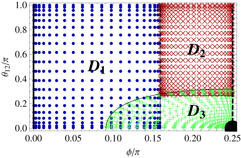
Figure 1: (Color online). This is the arrangement of grid points of the three domains at a constant value of $\rho$ in $\phi$ and $\theta_{12}$ coordinates for $n=20$. Note that the point density becomes larger at the boundary of each subdomain and that no grid points sit on the Coulomb singularities. The blue circles, red crosses, and green pluses belong to domains $D_{1}$, $D_{2}$, and $D_{3}$, respectively. $D_{1}$ and $D_{2}$ are rectangular domains, while $D_{3}$ has the curved boundary in $\phi$, $\theta_{12}$ coordinates but is rectangular in $\zeta$, $\beta_{12}$ coordinates. The electron-proton singularity occurs on the left side (solid line at $\phi=0$). The entire line corresponds to one physical point. The electron-electron singularity occurs at the lower right hand corner (solid disk at $\phi=\pi/4,\theta_{12}=0$). A line of symmetry falls on the right side (dashed line at $\phi=\pi/4$ where $r_{1}=r_{2}$).

VI Boundary conditions

VI.1 Internal boundary conditions

It is necessary to ensure continuity of the wave function and its normal derivative at internal boundaries. There are two ways in which the subdomains can touch: they can overlap or they can barely touch. For clarity, consider a one-dimensional problem with two domains. Let the first domain be domain $1$ and the second be domain $2$ with extrema ${\rm X}_{1,\textrm{min}}<{\rm X}_{2,\textrm{min}}\leq{\rm X}_{1,\textrm{max}}<{\rm X}_{2,\textrm{max}}$, where the $1$ and $2$ refer to domain number. The first case corresponds to ${\rm X}_{2,\textrm{min}}<{\rm X}_{1,\textrm{max}}$ and the second to ${\rm X}_{2,\textrm{min}}={\rm X}_{1,\textrm{max}}\equiv{\rm X}_{*}$. For both cases, exactly two conditions are needed to make the wave function and its derivative continuous. The simplest choice for the first case is

$$\psi_{1}[{\rm X}_{1,\textrm{max}}] = \psi_{2}[{\rm X}_{1,\textrm{max}}]$$ (53)

$$\psi_{1}[{\rm X}_{2,\textrm{min}}] = \psi_{2}[{\rm X}_{2,\textrm{min}}],$$ (54)

and for the second case is

$$\psi_{1}[{\rm X}_{*}] = \psi_{2}[{\rm X}_{*}]$$ (55)

$$\frac{d}{d{\rm X}}\psi_{1}[{\rm X}_{*}] = \frac{d}{d{\rm X}}\psi_{2}[{\rm X}_{*}].$$ (56)

For multi-dimensional grids, the situation is analogous. The conditions are applied on surfaces of overlap. In this case the derivatives are surface normal derivatives or any derivative not parallel to the boundary surface. On a discrete grid, a finite number of conditions are given which, in the limit of an infinitely fine mesh, would cover the entire surface. Additional discussion and illustrations of the technique are in Ref. Grabowski and Chernoff (2010).

VI.2 The symmetry condition

The Hamiltonian (see appendix A) is symmetric with respect to particle exchange ($r_{1}\leftrightarrow r_{2}$). Therefore, there are two types of eigenstates: those with symmetric spatial wave functions (singlets) and those with antisymmetric spatial wave functions (triplets). The radial wave functions $g_{\kappa ls}^{\nu}$ satisfying the appropriate symmetry must obey Eq. 18. More explicitly

$$0=\left\{\begin{array}[]{cc}\left.\frac{\partial{g_{\kappa ls}^{\nu}}}{\partial{\phi}}\right|_{\phi=\pi/4}=\left.\frac{\partial{g_{\kappa ls}^{\nu}}}{\partial{\beta_{12}}}\right|_{\beta_{12}=\pi/2}&\textrm{ if }\xi\textrm{ is even}\\ \left.g_{\kappa ls}^{\nu}\right|_{\phi=\pi/4}=\left.g_{\kappa ls}^{\nu}\right|_{\beta_{12}=\pi/2}&\textrm{ if }\xi\textrm{ is odd}\end{array}\right.,$$ (57)

where $\xi=\nu+\kappa+l+s$.

VII Energy and oscillator strength results

This article generalizes the pseudospectral methods previously developed for S states to the general angular momentum case, calculates oscillator strengths for transitions, and tests how different measures of wave function errors vary with resolution.

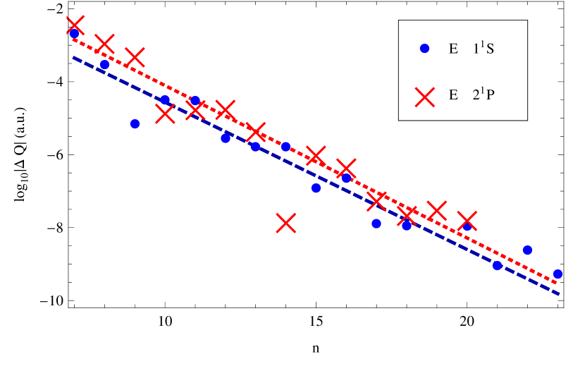
Figure 2: (Color online). The logarithm base 10 of the energy error ($\Delta Q$) of both the lowest energy S state and P state of helium. The dark blue circles are for the $1^{1}$S state and the light red crosses for the $2^{1}$P state with dashed blue and dotted red fits, respectively (see Tab. 1).

The most widely quoted number to ascertain convergence is the energy which gives a global measure of accuracy. Figure 2 shows the energy errors for the 1¹S and 2¹P states of helium. Here and throughout the results sections the high precision values of Drake Drake (1996) are taken to be exact. The energy error for both states decreases exponentially with resolution. Convergence for the S state is similar to that reported in Ref. Grabowski and Chernoff (2010) with slight differences related to a different choice of coordinates. The current calculation extends to basis size $n=23$ for S states and $n=20$ for P states instead of $n=14$ for only S states in Ref. Grabowski and Chernoff (2010).

A common feature of the energy convergence and all other convergence plots in this article is non-monotonic convergence. This method is not variational, so there is no reason to expect monotonic convergence. Calculated quantities can fall above or below their actual value, with error quasi-randomly determined by the exact grid point locations. The jumps decrease in magnitude as the resolution is increased.

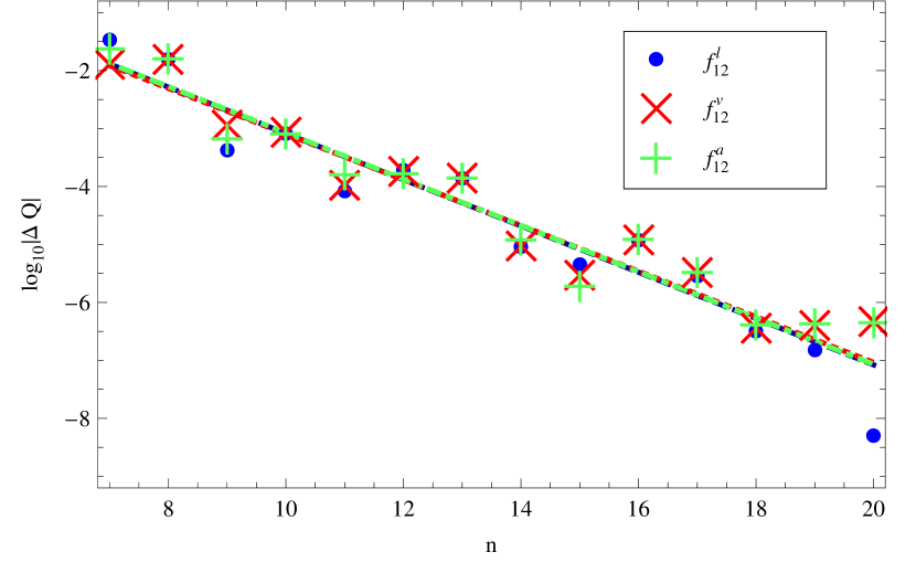
Figure 3: (Color online). The logarithm base 10 of the error ($\Delta Q$) in the oscillator strength of the $1^{1}$S $\to 2^{1}$P transition of helium. The dark blue circles are for the length form, the light red crosses are for the velocity form, and the green pluses for the acceleration form with dashed blue, dotted red, and dot-dashed green fits, respectively (see Tab. 1).

As described in Sec. IV, there are three commonly used forms for the oscillator strength. The length, velocity, and acceleration forms depend most strongly on the value of the wave function at positions in configuration space corresponding to large, medium, and small separations. Sometimes the relative errors are used to infer where the wave function is more or less accurate. It has been observed that for most variational calculations, the acceleration form tends to be much less accurate than the other two forms, suggesting errors in the wave function at small separation that have little effect on the variational energy. The length and velocity forms give results of roughly comparable accuracy.

The oscillator strength of the $1^{1}$S $\to 2^{1}$P transition was calculated using all three forms and Fig. 3 displays the errors. Here, all three forms give roughly the same results. At most resolutions the points lie nearly on top of one another and their fits are indistinguishable, indicating the wave function errors for small, medium, and large separations have roughly equal contributions to the numerically calculated oscillator strength. This may be due to the pseudospectral method’s equal treatment of all parts of configuration space.

It should be noted that the value used as the exact value Drake (1996) is given to seven decimal places. Consequently, the errors inferred for the highest resolution calculations in Fig. 3 are not too precise. There is little practical need for additional digits since a host of other effects including finite nuclear mass, relativistic, and quadrupole corrections would confound any hypothetical, experimental measurement of the oscillator strength to such high precision even if a perfect measurement could be made. Actual experiments struggle to obtain two percent precision Zitnik et al. (2003), an error larger than these effects.

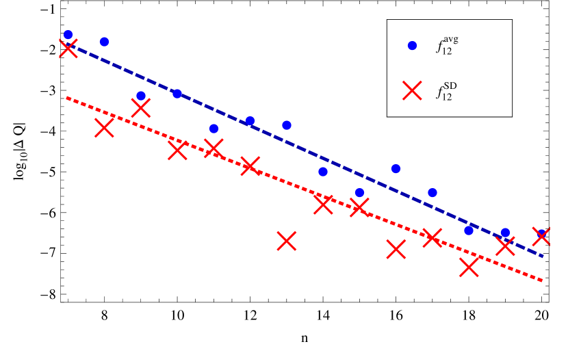
Figure 4: (Color online). The logarithm base 10 of the error ($\Delta Q$) in the average of the length, velocity, and acceleration forms of the oscillator strength (dark blue circles) and their standard deviation (light red crosses) for the $1^{1}$S $\to 2^{1}$P transition of helium, with dashed blue and dotted red fits, respectively (see Tab. 1).

As pointed out by Schiff et al. Schiff et al. (1971) and reviewed by Hibbert Hibbert (1975), the assumption that using the differences between the oscillator strength values from the different forms as a measure of the accuracy is not valid. Agreement is necessary but not sufficient. They suggest comparing calculated and extrapolated values. This latter procedure is not straightforward for a pseudospectral method with non-monotonic convergence. We present a similar suitable check. Fig. 4 shows the average and standard deviation of the error for the three forms as a function of resolution. The standard deviation is about an order of magnitude (with a large scatter about that factor of ten) less than the average error at low and moderate resolutions but the trend lines suggest that the standard deviation may be approaching the average at the higher resolutions. A possible explanation is that the calculation at the highest resolutions is starting to become sensitive to the wave function truncation (see appendix B.2). This destroys the expected equality between the forms and each form converges to its own incorrect asymptotic value. The individual errors and the standard deviation become comparable. So at $n=20$, we assume the standard deviation and total error are equal and get a value for the oscillator strength of $0.27616499(27)$ which compares favorably to Drake’s $0.2761647$ Drake (1996).

Table 1: The fit parameters to all the convergence plots of quantities $Q$ in this section.

$Q$	Figure	$A$	$\beta$
$E(1^{1}$S$)$	2	$2.5\times 10^{-9}$	0.40
$E(2^{1}$P$)$	2	$5.2\times 10^{-9}$	0.42
$f_{12}^{l}$	3	$8.4\times 10^{-8}$	0.40
$f_{12}^{v}$	3	$9.2\times 10^{-8}$	0.39
$f_{12}^{a}$	3	$8.6\times 10^{-8}$	0.40
$f_{12}^{avg}$	4	$8.7\times 10^{-8}$	0.40
$f_{12}^{SD}$	4	$2.2\times 10^{-8}$	0.34

All convergence data were fit to functions of the form $\Delta Q=A\times 10^{-\beta(n-20)}$ using the same procedure as in Ref. Grabowski and Chernoff (2010). Because of uncertainty in the errors for the largest resolutions ($n=19$ and $n=20$) these points were not used in the fits of $f_{12}^{l}$, $f_{12}^{v}$, $f_{12}^{a}$, and $f_{12}^{avg}$. The $\beta$ parameter, which corresponds to the slope of the fits in the convergence graphs is roughly the same for all fits, with the exception of the standard deviation of the oscillator strength forms. This behavior is consistent with our discussion of errors in the previous paragraph.

VIII Corrections to the Hamiltonian

Two small parameters appear in the full physical Hamiltonian: the ratio of the reduced mass of the electron-nucleus pair to the nuclear mass, $\mu/M=1.37074563559(58)\times 10^{-4}$ Mohr et al. (2008a, b) (for ⁴He) and the fine structure constant $\alpha=7.2973525376(50)\times 10^{-3}$ Mohr et al. (2008a, b). Here, the lowest order corrections in $\mu/M$ and $\alpha$ are considered. For very high-precision work, one needs the perturbative corrections in powers of each small quantity.

VIII.1 Finite nuclear mass correction

The nonrelativistic ($\alpha^{0}$) Hamiltonian for two-electron atoms is

$$\hat{H}_{\textrm{nr}}=\hat{H}_{0}+\hat{H}_{\textrm{cm}}+\hat{H}_{\textrm{mp}},$$ (58)

where $\hat{H}_{0}$ is the fixed-nucleus approximation to the Hamiltonian with the electron mass set to $\mu$, $\hat{H}_{\textrm{cm}}$ is the kinetic energy of the center of mass, and $\hat{H}_{\textrm{mp}}$ is the mass polarization term:

$$\hat{H}_{0} = \frac{1}{2}(p_{1}^{2}+p_{2}^{2})+\hat{V}$$ (59)

$$\hat{H}_{\textrm{cm}} = \frac{1}{2(M+2m_{e})}{p}_{\textrm{cm}}^{2}$$ (60)

$$\hat{H}_{\textrm{mp}} = \frac{1}{M}\mathbf{p}_{1}\cdot\mathbf{p}_{2},$$ (61)

where $\hat{V}$ is the potential energy operator, $m_{e}$ is the electron mass, $\mathbf{p}_{\textrm{cm}}$ is the momentum operator of the center of mass, and reduced mass atomic units ($\mu=1$) are being used. The second term is removed in center-of-mass coordinates and the last term provides the dominant nontrivial correction for finite nuclear mass (the trivial one being the scaling of the energy by $m_{e}/\mu$).

VIII.2 Relativistic corrections

The Schrödinger equation is a nonrelativistic approximation to the true equation of motion. The lowest order relativistic corrections enter at order $(\alpha^{2})$, as summarized in Ref. Fischer (1996) and repeated here. Note, all references in this article to orders in $\alpha$ are in Rydbergs. The Breit-Pauli Hamiltonian encapsulates the correction

$$\hat{H}_{\textrm{BP}}=\hat{H}_{\textrm{nr}}+\hat{H}_{\textrm{rel}},$$ (62)

where $\hat{H}_{\textrm{nr}}$ is the usual nonrelativistic Hamiltonian used in Schrödinger’s equation and $\hat{H}_{\textrm{rel}}$ is the lowest order relativistic correction. The latter can be further divided into non-fine-structure (NFS) and fine-structure (FS) contributions:

$$\hat{H}_{\textrm{NFS}} = \hat{H}_{\textrm{mass}}+\hat{H}_{\textrm{D}}+\hat{H}_{\textrm{SSC}}+\hat{H}_{\textrm{OO}}$$ (63)

$$\hat{H}_{\textrm{FS}} = \hat{H}_{\textrm{SO}}+\hat{H}_{\textrm{SOO}}+\hat{H}_{\textrm{SS}}.$$ (64)

The separate contributions to the Hamiltonian are the mass-velocity (mass), two-body Darwin (D), spin-spin contact (SSC), orbit-orbit (OO), spin-orbit (SO), spin-other-orbit (SOO), and the spin-spin (SS) terms. These are explicitly given by

$$\hat{H}_{\textrm{mass}} = -\frac{\alpha^{2}}{8}\sum_{i}p_{i}^{4}$$ (65)

$$\hat{H}_{\textrm{D}} = -\frac{\alpha^{2}Z}{8}\sum_{i}\nabla_{i}^{2}r_{i}^{-1}+\frac{\alpha^{2}}{4}\sum_{i<j}\nabla_{i}^{2}r_{ij}^{-1}$$ (66)

$$\hat{H}_{\textrm{SSC}} = -\frac{8\pi\alpha^{2}}{3}(\mathbf{s}_{1}\cdot\mathbf{s}_{2})\delta(\mathbf{r}_{12})$$ (67)

$$\hat{H}_{\textrm{OO}} = -\frac{\alpha^{2}}{2}\left(\frac{\mathbf{p}_{1}\cdot\mathbf{p}_{2}}{r_{12}}+\frac{\mathbf{r}_{12}(\mathbf{r}_{12}\cdot\mathbf{p}_{1})\cdot\mathbf{p}_{2}}{r_{12}^{3}}\right)$$ (68)

$$\hat{H}_{\textrm{SO}} = \frac{\alpha^{2}Z}{2}\sum_{i}\frac{\mathbf{\hat{l}}_{i}\cdot\mathbf{\hat{s}}_{i}}{r_{i}^{3}}$$ (69)

$$\hat{H}_{\textrm{SOO}} = -\frac{\alpha^{2}}{2}\sum_{i\neq j}\left(\frac{\mathbf{r}_{ij}}{r_{ij}^{3}}\times\mathbf{p}_{i}\right)\cdot(\mathbf{s}_{i}+2\mathbf{s}_{j})$$ (70)

$$\hat{H}_{\textrm{SS}} = \frac{\alpha^{2}}{r_{12}^{3}}\left(\mathbf{s}_{1}\cdot\mathbf{s}_{2}-\frac{3}{r_{12}^{2}}(\mathbf{s}_{1}\cdot\mathbf{r}_{12})(\mathbf{s}_{2}\cdot\mathbf{r}_{12})\right),$$ (71)

where $i$ and $j$ can be 1 or 2, $\mathbf{p}_{i}$ and $\mathbf{r}_{i}$ are the momentum and position of the $i$th electron with respect to the nucleus, respectively, $\mathbf{r}_{12}$ is the vector pointing from the first electron to the second, and $\mathbf{\hat{s}}_{i}$ and $\mathbf{\hat{l}}_{i}$ are the one-electron spin and angular momentum operators of the $i$th electron, respectively. The last three Hamiltonian terms are zero for ¹S states due to symmetry considerations.

There are many higher order terms (see Refs. Drake (1999); Drake and Morton (2007); Drake and Yan (2008); Pachucki and Yerokhin (2011a)) but these are not considered here.

IX Mass polarization and relativistic correction calculations

The mass polarization and low order relativistic corrections to the nonrelativistic Hamiltonian have been known for some time Bethe and Salpeter (1957). The main challenge in calculating these terms is finding adequate unperturbed wave functions. Early calculations Kinoshita (1957); Kabir and Salpeter (1957); Sucher (1958); Araki et al. (1959) were critical for comparing experimental and theoretical energies, confirming that Schrödinger’s equation is correct in the nonrelativistic limit for helium.

The development of computers enabled Pekeris and coworkers Pekeris (1958, 1959); Schiff et al. (1965) and others Schwartz (1961, 1964); Hambro (1972); Lewis and Serafino (1978); Davis and Chung (1982) to reach theoretical uncertainties in the energy of about $10^{-2}$ cm^-1. Such precision and the resulting precision in the wave function allowed Lewis and Serafino Lewis and Serafino (1978) to calculate the fine structure constant from experimental measurements of the $2^{3}$P splitting. They obtained $\alpha^{-1}=137.03608(13)$ with an estimated uncertainty only surpassed at the time by the measurements of the electron anomalous magnetic moment $(g-2)$ (by a factor of two) and the ac Josephson experiments (by a factor of four).

Drake and collaborators Drake (1987); Drake and Yan (1992); Yan and Drake (1995); Drake and Goldman (1999); Drake (1999, 2002, 2004) and Pachucki and collaborators Pachucki (1998); Pachucki and Sapirstein (2000, 2002, 2003); Pachucki (2006a, b, c); Pachucki and Yerokhin (2009, 2010); Pachucki and Yerokhin (2011a, b) have pushed relativistic corrections for regular helium up to order $\alpha^{5}$ and beyond using a Hylleraas Hylleraas (1929) type basis. Drake Drake (2002) matched theoretical and observed energy differences in the $J=0,1$ splitting of the $2^{3}$P state and determined $\alpha^{-1}=137.0359893(23)$. Drake cited a difference with the $g-2$ result $137.0359996(8)$ but agreement with the ac Josephson result $137.0359872(43)$ Drake (2002). However, a similar calculation of his using the observed $J=1,2$ splitting gives an unreasonable value Drake (2002). Pachucki and collaborators have resolved the issue by finding errors in $\alpha^{5}$ terms and by increasing the error estimate due to $\alpha^{6}$ terms. Their most recent determination is $\alpha^{-1}=137.03599955(64)(4)(368)$, where the first error is experimental, the second numerical, and the third is their estimated error from higher order terms Pachucki and Yerokhin (2011a). This value agrees with the latest $g-2$ results but is not as precise Pachucki and Yerokhin (2011a).

An alternative approach is to use an even simpler basis, with surprisingly accurate results. Korobov and collaborators have used an exponential basis (see Refs. Thakkar and Smith (1977); Frolov and Jr (1995)) to calculate very precise helium Korobov and Korobov (1999); Korobov (2000); Korobov and Yelkhovsky (2001); Korobov (2002a, b, 2004) (up to order $\alpha^{4}$) and anti-protonic helium Korobov et al. (1999); Korobov and Bakalov (2001); Korobov (2003, 2006); Korobov and Tsogbayar (2007); Korobov (2008); Korobov and Zhong (2009a, b) (up to order $\alpha^{5}$) electronic energies. The latter calculations have been used for the CODATA06 Mohr et al. (2008a, b) recommended value of the electron-to-(anti)proton mass ratio.

X Expectation values

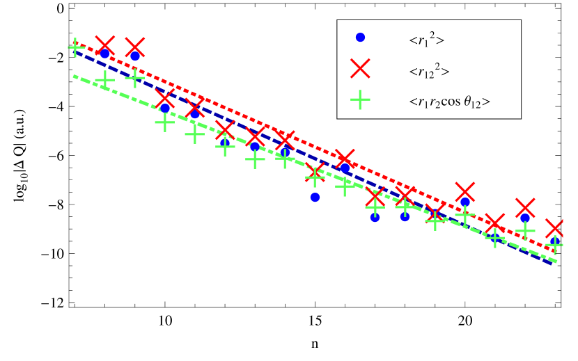
Figure 5: (Color online). The logarithm base 10 of the error ($\Delta Q$) in the expectation values of operators that scale as $\rho^{2}$ for helium. The dark blue circles are for $\langle r_{1}^{2}\rangle$, the light red crosses are for $\langle r_{12}^{2}\rangle$, and the green pluses are for $\langle r_{1}r_{2}\cos\theta_{12}\rangle$ with dashed blue, dotted red, and dot-dashed green fits, respectively (see Tab. 2).

The aim of this section is to test the pseudospectral method’s ability to represent the wave function in different parts of configuration space and to compare the convergence rates of the errors with that of the energies and oscillator strengths. For a representative set of calculations consider the expectation values of the operators needed for leading order relativistic (Sec. VIII.2) and finite nuclear mass (Sec. VIII.1) corrections, for the oscillator strength sum rules (Eqs. 30-33), interparticle distances, $\langle\hat{V}\rangle$, and $\langle\hat{V}^{2}\rangle$. These expectation values test different parts of the wave function as well as different types of operators. They are organized by the weighting of the wave function and used to draw inferences about local errors.

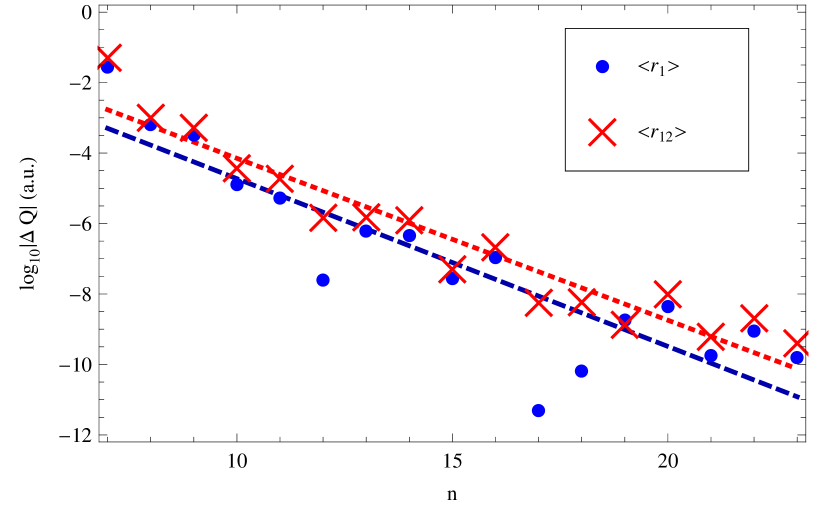
Figure 6: (Color online). The logarithm base 10 of the error ($\Delta Q$) in the expectation values of operators that scale as $\rho$ for helium. The dark blue circles are for $\langle r_{1}\rangle$ and the light red crosses are for $\langle r_{12}\rangle$ with dashed blue and dotted red fits, respectively (see Tab. 2).

Figure 5 displays results for expectation values related to sum rule $S(-1)$ (Eq. 30), i.e. quantities scaling like $\rho^{2}$. These calculations are somewhat more sensitive to the wave function at large separation than, say, the normalization integral. In addition, they focus on parts of coordinate space which have low resolution compared to the coverage near the singularities. High accuracy is found for all three cases.

Figure 6 displays results for expectation values of operators scaling like $\rho$ similar to the length form of the oscillator strength. Higher accuracy is obtained here than for the oscillator strength at equivalent resolutions. This can be explained by the smaller length scale set by the higher energy of the P state, which enters only into the oscillator strength calculations. So a greater resolution is needed for the same accuracy.

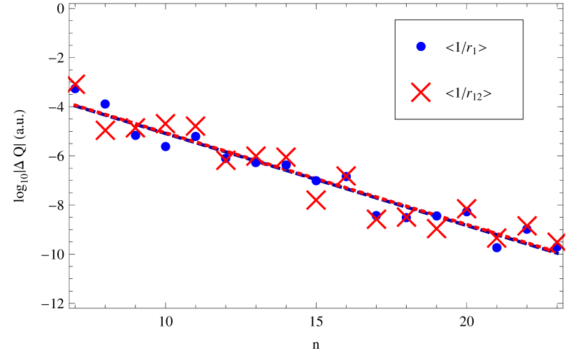
Figure 7: (Color online). The logarithm base 10 of the error ($\Delta Q$) in the expectation values of operators that scale as $1/\rho$ for helium. The dark blue circles are for $\langle 1/r_{1}\rangle$ and the light red crosses are for $\langle 1/r_{12}\rangle$ with dashed blue and dotted red fits, respectively (see Tab. 2).

Figure 7 displays results for expectation values related to the potential energy of charged particles, i.e. quantities scaling like $1/\rho$. This probes the treatment of the singularities. The high degree of accuracy is evidence that these singularities have been treated correctly.

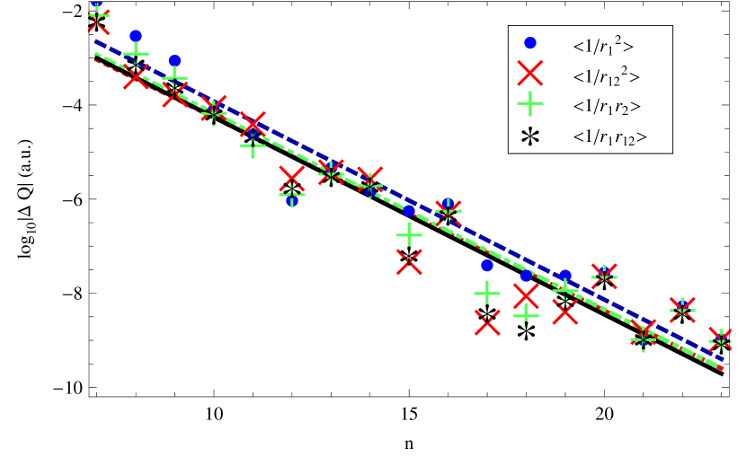
Figure 8: (Color online). The logarithm base 10 of the error ($\Delta Q$) in the expectation values of operators that scale as $1/\rho^{2}$ for helium. The dark blue circles are for $\langle 1/r_{1}^{2}\rangle$, the light red crosses are for $\langle 1/r_{12}^{2}\rangle$, the green pluses are for $\langle 1/r_{1}r_{2}\rangle$, and the black stars are for $\langle 1/r_{1}r_{12}\rangle$ with dashed blue, dotted red, dot-dashed green, and solid black fits, respectively (see Tab. 2).

Figure 8 displays results for expectation values related to the square of the potential energy, i.e. quantities scaling like $1/\rho^{2}$. These operators emphasize the singularities even further. One may expect that at a high enough inverse power of $\rho$ that the effect of the Fock logarithm become important and slow down convergence, but no evidence of that effect is apparent.

Even the expectation values of delta functions, related to sum rule $S(2)$ (Eq. 33), the Darwin term $\hat{H}_{\textrm{D}}$ (Eq. 66), and the spin-spin contact term $\hat{H}_{\textrm{SSC}}$ (Eq. 67), which are most sensitive to the Kato cusp conditions Kato (1957) have the same convergence properties (See Fig. 9). This provides evidence that our choices of coordinates allowed the pseudospectral method to deduce and represent the solution in the vicinity of a cusp. It also shows that if one can handle the non-analyticities of the matrix element by hand, as is possible for delta functions (see appendix B.3), one can still have exponentially fast convergence.

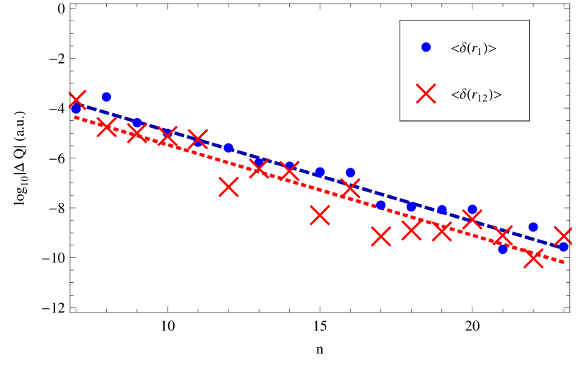
Figure 9: (Color online). The logarithm base 10 of the error ($\Delta Q$) in the expectation values of delta function operators for helium. The dark blue circles are for $\langle\delta(r_{1})\rangle$ and the light red crosses are for $\langle\delta(r_{12})\rangle$ with dashed blue and dotted red fits, respectively (see Tab. 2).

The error in the mass polarization $\hat{H}_{\textrm{mp}}$ (Eq. 61), used for the finite-nuclear mass correction and the calculation of the sum rule $S(1)$ (Eq. 32), and the orbit-orbit terms $\hat{H}_{\textrm{OO}}$ (Eq. 68), i.e. quadratic momentum contributions, are shown in Fig. 10. Calculations of derivatives (needed to form the appropriate operators) appear to be just as accurate as the function values, even when they are most strongly weighted close to the electron-electron cusp, as is the case for the orbit-orbit interaction.

The exponential rate of convergence and the magnitude of the errors are roughly the same in all the calculations of expectation values in Figs. 5-10. This is reflected in the fits (see Tab. 2).

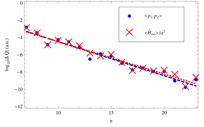
Figure 10: (Color online). The logarithm base 10 of the error ($\Delta Q$) in the expectation values of the mass polarization and the orbit-orbit interaction operators for helium. The dark blue circles are for $\langle\mathbf{p}_{1}\cdot\mathbf{p}_{2}\rangle$ and the light red crosses are for $\langle\hat{H}_{\textrm{OO}}\rangle/\alpha^{2}$ with dashed blue and dotted red fits, respectively (see Tab. 2).

These errors decrease until they reach roughly the level of error produced by truncating the wave function (see Sec. B) at the highest resolutions. The only easily discernible differences are at low resolution for which the representation of the wave function at large $\rho$ is certainly poor. It is unsurprising that the expectation values that scale as $\rho^{2}$ and $\rho$ have larger errors at low resolution due to the scarcity of points in the asymptotic tail of the wave function.

Table 2: The fit parameters to all the convergence plots of quantities $Q$ in this section.

$Q$	Figure	$A$	$\beta$
$\langle r_{1}^{2}\rangle$	5	$3.3\times 10^{-11}$	0.54
$\langle r_{12}^{2}\rangle$	5	$1.2\times 10^{-10}$	0.53
$\langle\mathbf{r_{1}}\cdot\mathbf{r_{2}}\rangle$	5	$4.9\times 10^{-11}$	0.47
$\langle r_{1}\rangle$	6	$1.2\times 10^{-11}$	0.48
$\langle r_{12}\rangle$	6	$7.5\times 10^{-11}$	0.46
$\langle 1/r_{1}\rangle$	7	$1.1\times 10^{-10}$	0.37
$\langle 1/r_{12}\rangle$	7	$1.2\times 10^{-10}$	0.37
$\langle 1/r_{1}^{2}\rangle$	8	$7.1\times 10^{-10}$	0.36
$\langle 1/r_{12}^{2}\rangle$	8	$3.1\times 10^{-10}$	0.38
$\langle 1/r_{1}r_{2}\rangle$	8	$3.9\times 10^{-10}$	0.37
$\langle 1/r_{1}r_{12}\rangle$	8	$2.6\times 10^{-10}$	0.37
$\langle\delta(r_{1})\rangle$	9	$2.4\times 10^{-10}$	0.36
$\langle\delta(r_{12})\rangle$	9	$6.5\times 10^{-11}$	0.36
$\langle\mathbf{p}_{1}\cdot\mathbf{p}_{2}\rangle$	10	$2.4\times 10^{-10}$	0.39
$\langle\hat{H}_{\textrm{OO}}\rangle/\alpha^{2}$	10	$4.3\times 10^{-10}$	0.38

All convergence data were fit to functions of the form $A\times 10^{-\beta(n-23)}$ using the same procedure as in Ref. Grabowski and Chernoff (2010). The fit parameters are shown in Tab. 2. The most striking feature is how similar the magnitudes of the errors are at $n=23$. Also, the exponential parameter $\beta$ is roughly the same for all expectation values and the energies and oscillator strengths (see Tab. 1) with the differences already discussed. Indeed, as one increases resolution one increases the accuracy of all expectation values or oscillator strengths by roughly the same amount.

The contributions to the total energy of the ground state of ⁴He are summarized in Tab. 3. The values from both this work and Drake’s Drake (1996) are given. For a wave function with a much lower precision in its eigenvalue (nine decimal places compared to fifteen), nearly the same precision is obtained for the corrections to this eigenvalue.

Table 3: The energy contributions to the ground state of ⁴He. These data use values of the physical constants $1/\alpha=137.035999679$ and $m_{e}/m_{\alpha}=0.000137093355571$, where $\alpha$ is the fine-structure constant, $m_{e}$ is the mass of the electron, and $m_{\alpha}$ is the mass of an alpha particle Mohr et al. (2008a, b). The errors do not include the uncertainties in these values.

Energy	This Work	Drake Drake (1996)
$\langle\hat{H}_{0}\rangle$	-2.9037243764(8)	-2.9037243770341195
$\langle\hat{H}_{\textrm{mass}}\rangle$		$-7.2006570459(3)\times 10^{-4}$
$\langle\hat{H}_{\textrm{OO}}\rangle$	$-7.4069807(1)\times 10^{-6}$	$-7.40698061439(5)\times 10^{-6}$
$\langle\hat{H}_{\textrm{D}}\rangle$	$5.879572027(5)\times 10^{-4}$	$5.8795720265(4)\times 10^{-4}$
$\langle\hat{H}_{\textrm{SSC}}\rangle$	$3.55818982(1)\times 10^{-5}$	$3.558189840(7)\times 10^{-5}$
$\langle\hat{H}_{\textrm{mp}}\rangle$	$2.18103579(2)\times 10^{-5}$	$2.1810357753732\times 10^{-5}$

XI Conclusions

We developed a general prescription for choosing coordinates and subdomains for a pseudospectral treatment of partial differential equations in the presence of physical and coordinate-related singularities. This prescription was applied to Schrödinger’s equation for helium to determine the fully correlated wave function. The treatment accounts for two-body but not three-body coalescences. Other problems with Coulomb singularities can now be tackled with this method.

We explored the fidelity of the pseudospectral method’s results. The method attained exponentially fast convergence for a wide selection of expectation values and matrix elements like the oscillator strength. Variational approaches minimize energy-weighted errors but generally do not yield comparable results for other operators. In contrast, we found that the pseudospectral method produced errors and convergence rates that were very similar for all the quantities studied including energy.

The approach should be widely applicable. No fine tuning was done to improve convergence other than ensuring non-analytic behavior was treated properly. The numerical method we developed was capable of solving the large matrix problems with modest computational resources. The calculations were pushed to the limits of double precision arithmetic. Higher precision floating point arithmetic will be necessary to go further.

This work generalized our previous treatment from S to P states and demonstrated the calculation of a variety of matrix elements. It can be further extended to higher angular momenta in a straightforward manner, albeit at larger computational cost.

The oscillator strength of the helium $1^{1}$S $\to 2^{1}$P transition was calculated to about the same accuracy as the most accurate value in the literature Drake (1996) and was found to agree to the expected precision.

Appendix A Bhatia and Temkin Hamiltonian

Bhatia and Temkin Bhatia and Temkin (1964) derived and we checked the following explicit expressions that make up the Hamiltonian in their three-three splitting:

$$\hat{H}_{S} = -\frac{1}{2}\sum_{i=1}^{2}\frac{1}{r_{i}^{2}}\left(\frac{\partial}{\partial{r_{i}}}r_{i}^{2}\frac{\partial}{\partial{r_{i}}}+\frac{1}{\sin\theta_{12}}\frac{\partial}{\partial{\theta_{12}}}\sin\theta_{12}\frac{\partial}{\partial{\theta_{12}}}\right)+\hat{V}$$ (72)

$$\hat{V} = -\frac{Z}{r_{1}}-\frac{Z}{r_{2}}+\frac{1}{r_{12}}$$ (73)

$$\hat{H}_{\nu,\kappa,-1}^{\gamma} = (1-\delta_{0\kappa}-\delta_{1\kappa}+(-1)^{j}\delta_{2\kappa})h_{\nu}^{\gamma}B_{l\kappa,-1}\left\{\begin{array}[]{ll}\cot\theta_{12}&\textrm{ if }\nu=\gamma\\ (-1)^{\nu}&\textrm{ if }\nu\neq\gamma\end{array}\right.$$ (76)

$$\hat{H}_{\nu\kappa 0}^{\gamma} = h_{\nu}^{\gamma}\left\{\begin{array}[]{ll}2\frac{l(l+1)-\kappa^{2}}{\sin\theta_{12}}+\kappa^{2}\sin\theta_{12}-\gamma\cot\theta_{12}l(l+1)\delta_{1\kappa}&\textrm{ if }\nu=\gamma\\ \nu\kappa(2\cos\theta_{12}+4\sin\theta_{12}\frac{\partial}{\partial{\theta_{12}}})-l(l+1)\delta_{1\kappa}&\textrm{ if }\nu\neq\gamma\end{array}\right.$$ (79)

$$\hat{H}_{\nu\kappa 1}^{\gamma} = (1-\nu\delta_{0\kappa})h_{\nu}^{\gamma}B_{l,\kappa+2,1}\left\{\begin{array}[]{ll}\cot\theta_{12}&\textrm{ if }\nu=\gamma\\ (-1)^{\gamma}&\textrm{ if }\nu\neq\gamma\end{array}\right.$$ (82)

$$h_{\nu}^{\gamma} = \frac{1}{8\sin\theta_{12}}\left(\frac{1}{r_{2}^{2}}+\frac{\nu\gamma}{r_{1}^{2}}\right)$$ (83)

$$B_{l\kappa n} = (1+\delta_{2\kappa}(\sqrt{2}-1))^{n}\sqrt{(l-\kappa+1)(l-\kappa+2)(l+\kappa)(l+\kappa-1)}.$$ (84)

Appendix B Matrix methods

B.1 Formalism

To solve for the wave function with given $k$, $l$ and $s$ and any $m$, one must calculate the values of $g_{\kappa ls}^{\nu}$ for each $\kappa$ and $\nu$ that enters the summation in Eq. 17. In this section we suppress writing $k$, $l$, $s$ and $m$ indices; only $\nu$ and $\kappa$ will appear explicitly. There are two types of conditions which must be satisfied: the Schrödinger equation and the boundary conditions.

The $\kappa$ values of interest are $\kappa_{m}$, the minimum value, $\kappa_{m}+2$, … up to $\kappa_{M}$, the maximum value. The minimum and maximum values depend upon parity, $l$ and $\nu$ (for notational clarity omitted). The minimum $\kappa$ is

$$\kappa_{m}=\nu+\frac{1}{2}(1-(-1)^{\nu}k)$$ (85)

and the maximum is

$$\kappa_{M}=2\left\lfloor\frac{l}{2}\right\rfloor-\frac{(-1)^{l}}{2}(1-k).$$ (86)

Let $g_{\kappa}^{\nu}$ stand for all the grid point values for a given $\nu$ and $\kappa$. Assemble these in a column vector form that enumerates the full set of $\kappa$ for a fixed $\nu$

$$g^{\nu}=\left(\begin{array}[]{c}g_{\kappa_{m}}^{\nu}\\ g_{\kappa_{m}+2}^{\nu}\\ \vdots\\ g_{\kappa_{M}}^{\nu}\end{array}\right).$$ (87)

The length of this column vector is ${\tilde{l}}=1+(\kappa_{M}-\kappa_{m})/2$, which takes on the values $\lfloor l/2\rfloor$ or $\lceil l/2\rceil$. The size of the matrix problem increases linearly with $l$.

The Schrödinger equation can be represented in matrix form:

$$\left(\begin{array}[]{cc}H_{0}^{0}+(H_{S}-E)\mathbf{1}&H_{1}^{0}\\ H_{0}^{1}&H_{1}^{1}+(H_{S}-E)\mathbf{1}\end{array}\right)\left(\begin{array}[]{c}g^{0}\\ g^{1}\end{array}\right)=0,$$ (88)

where $E$ is the energy, $H_{S}$ is the S-wave part and $H_{\nu}^{\gamma}$ the non-S-wave part of the Hamiltonian, and $\mathbf{1}$ is the identity matrix. $H_{\nu}^{\gamma}$ and $\mathbf{1}$ are square matrices with dimensions ${\tilde{l}}\times{\tilde{l}}$. Explicitly, $H_{\nu}^{\gamma}$ is the tridiagonal matrix

$$H_{\nu}^{\gamma}=\left(\begin{array}[]{ccccc}H_{\nu,\kappa_{m},0}^{\gamma}&H_{\nu,\kappa_{m},1}^{\gamma}&0&\cdots&0\\ H_{\nu,\kappa_{m}+2,-1}^{\gamma}&H_{\nu,\kappa_{m}+2,0}^{\gamma}&H_{\nu,\kappa_{m}+2,1}^{\gamma}&\ddots&\vdots\\ 0&H_{\nu,\kappa_{m}+4,-1}^{\gamma}&H_{\nu,\kappa_{m}+4,0}^{\gamma}&\ddots&0\\ \vdots&\ddots&\ddots&\ddots&H_{\nu,\kappa_{M}-2,1}^{\gamma}\\ 0&\cdots&0&H_{\nu,\kappa_{M},-1}^{\gamma}&H_{\nu,\kappa_{M},0}^{\gamma}\end{array}\right).$$ (89)

The third subscript on the $H^{\gamma}_{\nu,\kappa,n}$ labels the coupling of the individual $g$ functions in $\kappa$. For the S and P states calculated in this article, $H_{\nu}^{\gamma}$ is only a one by one matrix.

The pseudospectral matrices $H_{S}$ and $H_{\nu,\kappa,n}^{\gamma}$ (for specific $\nu$, $\kappa$, $\gamma$ and $n$) are constructed from Eq. 6 with $\hat{H}$ replaced by $\hat{H}_{S}$ or $\hat{H}_{\nu\kappa n}^{\gamma}$, respectively (see appendix A for explicit forms of these operators). These single elements are large matrices having dimensions set by the number of grid points. For multiple subdomains, they are block diagonal. The pseudospectral matrix is constructed for the subdomain’s grid points. The number of columns and rows of an element equals the total number of grid points in all the subdomains.

The boundary conditions can be written as

$$\left(\begin{array}[]{cc}B_{0}&0\\ 0&B_{1}\end{array}\right)\left(\begin{array}[]{c}g^{0}\\ g^{1}\end{array}\right)=0,$$ (90)

where

$$B_{\nu}=\left(\begin{array}[]{cccc}B_{\nu}^{j_{m}}&0&\cdots&0\\ 0&B_{\nu}^{j_{m+2}}&\ddots&\vdots\\ \vdots&\ddots&\ddots&0\\ 0&\cdots&0&B_{\nu}^{j_{M}}\end{array}\right),$$ (91)

is a diagonal matrix of the same size as $H_{\nu}^{\gamma}$, and $j_{m}=\nu+\kappa_{m}+l+s$ and $j_{M}=\nu+\kappa_{M}+l+s$. Each $B_{\nu}^{j}$ is a rectangular matrix of the same width as $H_{\nu\kappa n}^{\gamma}$, but a smaller height corresponding to the number of grid points near internal boundaries or where a symmetry condition holds. If $j$ is even (odd) $B_{\nu}^{j}$ enforces zero derivative (value) along the symmetry plane.

As in Ref. Grabowski and Chernoff (2010) each of the $B_{\nu}^{j}$ matrices can be split into two sub-matrices

$$B_{\nu}^{j}=\left(B_{\nu 1}^{j}B_{\nu 2}^{j}\right),$$ (92)

and similarly splitting the vector $g_{\kappa}^{\nu}$

$$g_{\kappa}^{\nu}=\left(\begin{array}[]{c}g_{\kappa 1}^{\nu}\\ g_{\kappa 2}^{\nu}\end{array}\right),$$ (93)

yields the equation

$$B_{\nu 1}^{j}g_{\kappa 1}^{\nu}+B_{\nu 2}^{j}g_{\kappa 2}^{\nu}=0,$$ (94)

where the vector and matrix have been ordered so that the index 1 refers to the $n_{b}$ boundary points and the index 2 refers to the $n_{i}$ interior points. The grid point nearest to the boundary, at which an explicit boundary condition is given is considered a boundary point. $B_{\nu 1}^{j}$ is an $n_{b}$ by $n_{b}$ matrix and $B_{\nu 2}^{j}$ is an $n_{b}$ by $n_{i}$ matrix. The total number of grid points is $n_{t}=n_{b}+n_{i}$.

Each $n_{t}$ by $n_{t}$ block of the Hamiltonian matrix $H_{\nu}^{\gamma}$ (Eq. 89) can be split in a similar way,

$$H_{\nu\kappa n}^{\gamma}=\begin{array}[]{c}n_{b}\{\\ n_{i}\{\end{array}\underbrace{\left(\begin{array}[]{c}H_{\nu\kappa n11}^{\gamma}\\ H_{\nu\kappa n21}^{\gamma}\end{array}\begin{array}[]{c}H_{\nu\kappa n12}^{\gamma}\\ H_{\nu\kappa n22}^{\gamma}\end{array}\right)}_{n_{b}+n_{i}}.$$ (95)

There are $n_{t}+n_{b}$ equations and $n_{t}$ unknowns ($g_{1}$ and $g_{2}$) as well as the eigenvalue. One could approximately solve these equations with singular value decomposition Press et al. (2007), but it is much faster to simply discard the first $n_{b}$ rows of each $H_{\nu\kappa n}^{\gamma}$ (one should still check after finding a solution that it approximately satisfies those rows of the matrix equation) and incorporate the boundary conditions into the remaining eigenvalue problem by replacing each $H_{\nu\kappa n}^{\gamma}$ with

$$H_{\nu\kappa n}^{\gamma}\to H_{\nu\kappa n22}^{\gamma}-H_{\nu\kappa n21}^{\gamma}(B_{\nu 1}^{j})^{-1}B_{\nu 2}^{j},$$ (96)

where $B_{\nu 1}^{j}$ has an inverse because all of its rows are linearly independent (otherwise more than one boundary condition would have been specified for a given boundary point). Calculating the inverse is computationally inexpensive since $n_{b}\ll n_{t}$. The eigenvector gives $g_{\kappa 2}^{\nu}$ and one solves for $g_{\kappa 1}^{\nu}$ with

$$g_{\kappa 1}^{\nu}=-(B_{\nu 1}^{j})^{-1}B_{\nu 2}^{j}g_{\kappa 2}^{\nu}.$$ (97)

Table 4: The matrix sizes $n_{m}$ and number of non-zero elements $n_{NZ}$ for each resolution $n$.

Resolution	1S States		1P States
$n$	$n_{m}$	$n_{NZ}$	$n_{m}$	$n_{NZ}$
7	1 512	182 952	3 024	573 720
8	2 352	381 024	4 704	1 204 448
9	3 456	722 304	6 912	2 297 276
10	4 860	1 273 320	9 720	4 069 800
11	6 600	2 118 600	13 200	6 798 440
12	8 712	3 362 832	17 424	10 826 640
13	11 232	5 133 024	22 464	16 571 568
14	14 196	7 580 664	28 392	24 531 416
15	17 640	10 883 880	35 280	35 292 600
16	21 600	15 249 600	43 200	49 536 960
17	26 112	20 915 712	52 224	68 048 960
18	31 212	28 153 224	62 424	91 722 888
19	36 936	37 268 424	73 872	121 570 056
20	43 320	48 605 040	86 640	158 726 000
21	50 400	62 546 400
22	58 212	79 517 592
23	66 792	99 987 624

B.2 Matrix Eigenvalue Solution

The number of grid points in each sub-domain, $\{x,\phi,\theta_{12}\}$ or $\{x,\zeta,\beta_{12}\}$, was $n_{t}=2n\times n\times n$; greater resolution is needed along the semi-infinite coordinate. This leads to a Hamiltonian matrix size of $n_{t}\times n_{t}$ for S states and $2n_{t}\times 2n_{t}$ for odd parity P states. After solving for boundary conditions with the above procedure, these are reduced to $n_{m}\times n_{m}$ and $2n_{m}\times 2n_{m}$, respectively, where $n_{m}=n_{i}=6n^{3}-12n^{2}+6n$. The number of non-zero elements $n_{NZ}$ scales as $n^{4}$. For $n=20$, this corresponds to 560 MB and 1.8 GB, respectively, of memory required to store the matrix. The sizes of the matrices and the number of non-zero elements is given in Tab. 4.

The method of inverse iteration Press et al. (2007) was used to find eigenvalues with a shift equal to the known eigenvalues plus $10^{-4}$ so that the matrix is not too singular. Each iteration requires a matrix solve. For the smaller matrices (up to $17,000\times 17,000$), these solves were performed using Mathematica’s Wolfram Research (2008) multifrontal matrix solve routine. This method is fast (eigenvalues can be calculated in about 10 minutes for that size) but $8$ GB of RAM was insufficient to do larger sizes. For larger matrices, the generalized minimal residual (GMRES) method of PETSc Balay et al. (2009, 2008, 1997) was used. The GMRES method produces a solution with the Krylov space of the matrix and is more memory efficient.

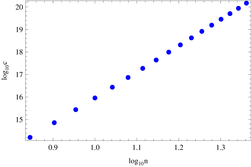
Figure 11: (Color online). A log-log plot of the spectral condition number $c$ of the pseudospectral matrices as a function of resolution.

Preconditioning is essential for solving large matrix problems. A measure of how hard a matrix problem is to solve (how fast a method converges) is the spectral condition number, defined as

$$c=\frac{|\lambda_{\textrm{max}}|}{|\lambda_{\textrm{min}}|},$$ (98)

where $\lambda_{\textrm{max}}$ and $\lambda_{\textrm{min}}$ are the eigenvalues with the largest and smallest magnitudes, respectively. The spectral condition numbers of pseudospectral matrices grow rather fast with increasing resolution Pfeiffer (2010); Fornberg (1996c). For the problem at hand, it is plotted versus resolution in Fig. 11. It starts out large and grows asymptotically as $n^{12}$. An ill-posed problem has a condition number which grows exponentially Teukolsky (2010). This problem is well-posed but in order to solve this system of equations preconditioning is necessary. A reasonable preconditioner is a matrix produced by a second order finite differencing scheme on the same set of grid points Pfeiffer (2010); Orszag (1980); Fornberg (1996c). The preconditioning matrix solves are further preconditioned with a block Jacobi preconditioner.

The modified Gramm-Schmidt procedure was used to orthogonalize the Krylov subspace. Furthermore, the GMRES restart parameter, $m$, needs to be very large for convergence, empirically, $m=1.3n_{m}^{3/4}$, where $n_{m}\times n_{m}$ is the matrix size. The computation time scales as $n_{m}^{3}$, which for the largest matrix size was about a day running on six 2 GHz processors. The eigenvalue solver is the slowest part of the entire computation.

All calculations were done with double precision arithmetic. This gives some minimum error in the calculated eigenstate. The effect is relatively big for the small exponential tail. The key observation is that the wave function no longer decreases at the theoretically expected asymptotic rate when it drops to about $10^{-8.7}$ of its maximum value, after which it takes on a seemingly random value less than this magnitude. This value is independent of resolution because of the limits of machine precision arithmetic. It is possible that the asymptotic tail could be better calculated with a better preconditioner.

The issue of the asymptotic behavior is important. Since a constant value for the wave function on a semi-infinite domain leads to divergent matrix elements, we set any value of the eigenvector below this threshold to zero.

B.3 Quadrature

In this article, it is necessary to calculate matrix elements of the form $\langle i|\hat{O}|j\rangle$, where $|i\rangle$ and $|j\rangle$ are two quantum states and $\hat{O}$ is some operator. This calculation requires numerical integration. Pseudospectral methods, by design, use quadrature points as the grid points. A one dimensional function $f[{\rm X}]$ can be numerically integrated from ${\rm X}=-1$ to ${\rm X}=1$ with weight function $g[{\rm X}]$ by

$$\int_{-1}^{1}f[{\rm X}]g[{\rm X}]d{\rm X}\approx\sum w_{i}f[{\rm X}^{i}],$$ (99)

where $w_{i}$ is the quadrature weight specific to the weighting function $g$ at grid point ${\rm X}^{i}$. This quadrature formula is exponentially accurate with increasing resolution if $f$ is smooth over the domain $-1\leq{\rm X}\leq 1$. The problems solved in this article are three-dimensional with three overlapping subdomains. A separate quadrature can be done in each sub-domain. This is illustrated for domain ${D}_{1}$ with coordinates $\{x,\phi,\theta_{12}\}$ and ranges $-1\leq x\leq 1$, $0\leq\phi\leq 1/2$, and $0\leq\theta_{12}\leq\pi$. Define

$${\rm X}_{1} = x$$ (100)

$${\rm X}_{2} = 4\phi-1$$ (101)

$${\rm X}_{3} = \frac{2\theta_{12}}{\pi}-1,$$ (102)

so that $-1\leq{\rm X}_{1},{\rm X}_{2},{\rm X}_{3}\leq 1$. Integrals over ${D}_{1}$ use three-dimensional sums analogous to Eq. 99. Since the ranges are fixed, the order of nesting is immaterial. To satisfy the requirement that $f$ is smooth (up to the logarithmic singularity at $\rho=0$), choose $g=1$, which corresponds to Legendre quadrature points, which are used for all calculations in this article instead of Chebyshev which were used in Ref. Grabowski and Chernoff (2010).

If all the subdomains are non-overlapping, then the above scheme is sufficient for all integrals. However, no set of non-overlapping subdomains for which $f$ is smooth could be found. A method is needed for handling overlapping regions, which the above scheme double counts if a quadrature is performed in each sub-domain. For these regions, an interpolation was performed to two new $2n\times n\times n$ grids spanning the overlap regions, shown in Fig 12. For the pseudospectral method, interpolation is done to the same order as the grid size. A quadrature can then be done over the overlap regions, which are used to correct the overall integration.

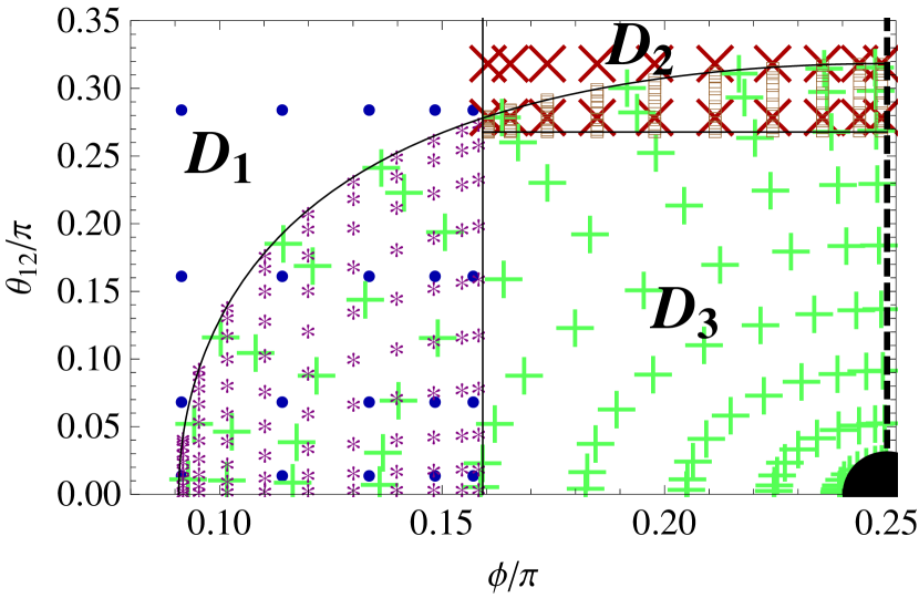
Figure 12: (Color online). This is the arrangement of grid points of the three domains at a constant value of $\rho$ in $\phi$ and $\theta_{12}$ coordinates for $n=10$. As in Fig. 1, the blue circles, red crosses, and green pluses belong to domains $D_{1}$, $D_{2}$, and $D_{3}$, respectively. Also shown are the overlap grid points in $D_{1}\cap D_{3}$ (purple stars) and $D_{2}\cap D_{3}$ (brown squares). The electron-electron singularity is visible at the lower right hand corner (solid disk at $\phi=\pi/4,\theta_{12}=0$) as well as the line of symmetry on the right side (dashed line at $\phi=\pi/4$ where $r_{1}=r_{2}$).

The overlap region is divided into two subdomains

$${D}_{13} = {D}_{1}\cap{D}_{3}$$ (103)

$${D}_{23} = {D}_{2}\cap{D}_{3}.$$ (104)

These subdomains satisfy

$$\begin{array}[]{lccc}D_{13}:&-1\leq x\leq 1,&\phi_{\textrm{min}}\leq\phi\leq\frac{1}{2},&0\leq\theta_{12}\leq\theta_{12,\textrm{max}}[\phi]\\ D_{23}:&-1\leq x\leq 1,&\frac{1}{2}\leq\phi\leq\frac{\pi}{4},&\arccos\frac{2}{3}\leq\theta_{12}\leq\theta_{12,\textrm{max}}[\phi],\end{array}$$ (105)

where $\phi_{\textrm{min}}=\pi/4-1/2$ is determined by $\zeta=1/2$ and $\theta_{12}=0$ and $\theta_{12,\textrm{max}}[\phi]=\arccos[\cos 1\csc 2\phi]$ is determined by $\zeta=1/2$. One defines appropriate $\{{\rm X}_{1},{\rm X}_{2},{\rm X}_{3}\}$. For example, in $D_{13}$

$${\rm X}_{1} = x$$ (106)

$${\rm X}_{2} = 2\left(\frac{\phi-\phi_{\textrm{min}}}{\frac{1}{2}-\phi_{\textrm{min}}}\right)-1$$ (107)

$${\rm X}_{3} = 2\theta_{12,\textrm{max}}[\phi]\theta_{12}-1.$$ (108)

Now one calculates the nested sum with ${\rm X}_{3}$ innermost since the range of $\theta_{12}$ depends upon $\phi$.

The function values at the points necessary for the quadrature $\{x^{j_{1}^{\prime}},\phi^{j_{2}^{\prime}},\theta_{12}^{j_{2}^{\prime}j_{3}^{\prime}}\}$ are calculated with interpolation

$$f[x^{j_{1}^{\prime}},\phi^{j_{2}^{\prime}},\theta_{12}^{j_{2}^{\prime}j_{3}^{\prime}}]\approx\sum_{J}f[x^{j_{1}},\phi^{j_{2}},\theta_{12}^{j_{3}}]{\cal C}_{J}[x^{j_{1}^{\prime}},\phi^{j_{2}^{\prime}},\theta_{12}^{j_{2}^{\prime}j_{3}^{\prime}}].$$ (109)

where ${\cal C}_{J}$ refers to the effective basis defined in Eq. 3 and $J=\{j_{1},j_{2},j_{3}\}$.

Sometimes $f$ involves a Dirac delta function. In such a case, one integrates out the delta function analytically. One is left with a two dimensional integral on the surface where the argument of the delta function is zero. This entails first interpolating to that surface using Eq. 109. One can then proceed normally with a two-dimensional quadrature.

Appendix C Calculating matrix elements with Bhatia and Temkin’s radial functions

C.1 Oscillator Strength

In the Bhatia and Temkin three-three splitting Bhatia and Temkin (1964), the matrix elements for an ¹S $\to{}^{1}$P oscillator strength transition are written:

$$\sum_{m}|\langle{}^{1}\textrm{S}|\hat{\mathbf{D}}|{}^{1}\textrm{P}m\rangle|^{2}=\left[\int d\tau g_{000}^{0}\left(d_{D}^{0}g_{110}^{0}+d_{D}^{1}g_{110}^{1}\right)\right]^{2},$$ (110)

where $d\tau=r_{1}^{2}r_{2}^{2}\sin\theta_{12}dr_{1}dr_{2}d\theta_{12}$, $\hat{\mathbf{D}}$ is one of the operators found inside the matrix elements of Eqs. 22 and the operators $d_{D}^{i}$ are given by

$$d_{\mathbf{R}}^{0} = (r_{1}+r_{2})\cos\frac{\theta_{12}}{2}$$ (111)

$$d_{\mathbf{R}}^{1} = (r_{1}-r_{2})\sin\frac{\theta_{12}}{2}$$ (112)

$$d_{\mathbf{P}}^{0} = \frac{(r_{1}+r_{2})(3+\cos\theta_{12})}{4r_{1}r_{2}\cos\frac{\theta_{12}}{2}}$$ (113)

$$+\cos\frac{\theta_{12}}{2}\left(\frac{\partial}{\partial{r_{1}}}+\frac{\partial}{\partial{r_{2}}}\right)$$

$$-\frac{(r_{1}+r_{2})\sin\frac{\theta_{12}}{2}}{r_{1}r_{2}}\frac{\partial}{\partial{\theta_{12}}}$$

$$d_{\mathbf{P}}^{1} = \frac{(r_{1}-r_{2})(-3+\cos\theta_{12})}{4r_{1}r_{2}\sin\frac{\theta_{12}}{2}}$$ (114)

$$+\sin\frac{\theta_{12}}{2}\left(\frac{\partial}{\partial{r_{1}}}-\frac{\partial}{\partial{r_{2}}}\right)$$

$$-\frac{(r_{1}-r_{2})\cos\frac{\theta_{12}}{2}}{r_{1}r_{2}}\frac{\partial}{\partial{\theta_{12}}}$$

$$d_{\mathbf{A}}^{0} = \frac{Z(r_{1}^{2}+r_{2}^{2})\cos\frac{\theta_{12}}{2}}{r_{1}^{2}r_{2}^{2}}$$ (115)

$$d_{\mathbf{A}}^{1} = \frac{Z(r_{1}^{2}-r_{2}^{2})\sin\frac{\theta_{12}}{2}}{r_{1}^{2}r_{2}^{2}}.$$ (116)

C.2 Expectation Values

Similarly, an expectation value for an S state is calculated by

$$\langle{}^{1}\textrm{S}|\hat{\mathbf{D}}|{}^{1}\textrm{S}\rangle=\int d\tau g^{0}_{000}d^{0}_{D}g^{0}_{000}.$$ (117)

Most of the operators $d^{0}_{D}$ used for expectation values in this article have trivial forms. We write here only the two most complicated ones:

$$d^{0}_{\mathbf{p}_{1}\cdot\mathbf{p}_{2}} = \frac{1}{r_{1}r_{2}}\left[\sin\theta_{12}\left(r_{1}\frac{\partial}{\partial{r_{1}}}+r_{2}\frac{\partial}{\partial{r_{2}}}\right)\frac{\partial}{\partial{\theta_{12}}}\right.$$ (118)

$$-r_{1}r_{2}\cos\theta_{12}\frac{\partial^{2}}{\partial{r_{1}}\partial{r_{2}}}+\cos\theta_{12}\frac{\partial^{2}}{\partial{\theta_{12}}^{2}}$$

$$\left.+\frac{1}{\sin\theta_{12}}\frac{\partial}{\partial{\theta_{12}}}\right]$$

$$d^{0}_{H_{OO}} = -\frac{\alpha^{2}}{2r_{12}^{3}}\left[\sin\theta_{12}\left(x_{12}\frac{\partial}{\partial{r_{1}}}+x_{21}\frac{\partial}{\partial{r_{2}}}\right)\frac{\partial}{\partial{\theta_{12}}}\right.$$ (119)

$$+r_{1}r_{2}z_{+}\frac{\partial^{2}}{\partial{r_{1}}\partial{r_{2}}}+z_{-}\frac{\partial^{2}}{\partial{\theta_{12}}^{2}}$$

$$\left.+\frac{r_{12}^{2}}{r_{1}r_{2}\sin\theta_{12}}\frac{\partial}{\partial{\theta_{12}}}\right],$$

where

$$x_{ij}=\frac{r_{i}^{2}+r_{12}^{2}-\mathbf{r}_{1}\cdot\mathbf{r}_{2}}{r_{j}}$$ (120)

and

$$z_{\pm}=(1\pm 3)\cos\theta_{12}(\cos\theta_{12}-\rho^{2}/2r_{1}r_{2})+\sin^{2}\theta_{12}.$$ (121)

All of these forms must be converted to the appropriate coordinates in each subdomain.

Appendix D History of Oscillator Calculations

Table LABEL:History1S2P-OscStrengths summarizes the last half century’s theoretical studies of the nonrelativistic, electric dipole oscillator strength. The prime criterion for inclusion in the Table is that a numerical value for the oscillator strength for the specific transition $1^{1}$S $\to 2^{1}$P be calculated and quoted. We do not indicate in this Table other transitions calculated even though these often constitute the bulk of a paper’s research results. In broadest terms, the entries illustrate progress in achieving higher accuracy for the specific transition and/or testing new methods designed to yield more extensive sets of bound-bound oscillator strengths.

Many methods appearing in Table LABEL:History1S2P-OscStrengths are variational and utilize the exact interaction potential of the nonrelativistic Hamiltonian Schiff and Pekeris (1964); Green et al. (1966); Weiss (1967); Chong and Benston (1968); Schiff et al. (1971); Kono and Hattori (1984); Cann and Thakkar (1992); Chen (1994, 1994); Yang (1997); Drake (1996). Variational methods are especially useful when electron correlation is important and ground state properties are sought. There are many strategies for selecting bases and suitable variational parameters. This flexibility may become cumbersome for the study of highly excited states if lower level states must be projected out as a preliminary step (e.g. if the trial wave function is not linear in the unknown parameters and one seeks to enforce orthogonality of the excited state with respect to lower states). Errors in the eigenproblem accumulate and higher levels are harder to find accurately, even when the wave function is linear in the variational parameters.

A general conclusion is that some basis choices do a better job representing the parts of the wave function critical to oscillator strength calculations. Configuration interaction (CI) calculations Schiff and Pekeris (1964); Brown (1969); Brown and Cortez (1972); Davis and Chung (1982); Chen (1994) converge but suffer from the absence of odd powers of the inter-electronic distance Drake (1999). Perimetric Pekeris (1958) coordinates Schiff et al. (1971); Drake (1996, 1999); Drake et al. (2002); Drake (2004); Drake and Morton (2007); Drake and Yan (2008) and Hylleraas Hylleraas (1929) coordinates Weiss (1967); Anderson and Weinhold (1974); Kono and Hattori (1984); Yang (1997) include terms of this sort. Systematic variational studies using bases incorporating the inter-electronic distance have yielded some of the more accurate calculations to date. A Hylleraas expansion is used by Drake who determined the oscillator strengths to seven decimal digits Drake (1996), the most precise calculations thus far, as well as some finite-nuclear-mass and relativistic corrections. At this stage further nonrelativistic calculations of the oscillator strength are probably less important than the inclusion of spin-orbit, mass polarization and low-order relativistic effects.

Expansions in terms of orthogonal functions often produce basis elements of increasing complexity. Alternatively, one can use larger numbers of simpler functions. One important example is the exponential basis Thakkar and Smith (1977); Frolov and Jr (1995) (exponential functions of $r_{1}$, $r_{2}$ and $r_{12}$), which has the great advantage of having an easy to calculate Hamiltonian matrix at the expense of violating cusp conditions. This basis was used by Cann and Thakkar Cann and Thakkar (1992) to get many different oscillator strengths for S $\to$ P and P $\to$ D transitions of helium-like atoms. They got the $1^{1}$S $\to 2^{1}$P oscillator strength correct to five decimal places.

The central field approximation Bethe and Salpeter (1957) is suitable when electrons are nearly uncorrelated and exchange effects are negligible. The essence of this approximation is twofold: (1) the multi-electron wave function is written in terms of products of one-electron functions and (2) each electron experiences a potential which is a function only of its distance to the nucleus. The omission of explicit inter-electronic coordinates hinders convergence but greatly simplifies the variational problem. Green et al. Green et al. (1966) produced tables of S $\to$ P and P $\to$ S transitions using the configuration interaction form for the wave functions.

There exist many different approximations to representing the fully correlated wavefunctions. Multiconfiguration Hartree-Fock recovers some but not all of the electron correlation energy and yields improved oscillator strengths compared to Hartree-Fock treatments Fischer (1974). The coupled cluster expansion (roughly analogous to a truncated form of configuration interaction) also yields better results Fernley et al. (1987).

Simplifications are frequently made to generate comprehensive but approximate oscillator strength databases. With this approach the physical as opposed to numerical errors may be difficult to gauge. For a two-electron atom the Hamiltonian may be written

$$\hat{H}_{0} \approx \hat{H}_{1}+\hat{H}_{2}$$ (122)

$$\hat{H}_{i} = \frac{p_{i}^{2}}{2}+U_{i}[r_{i}],$$ (123)

where $U_{i}$ accounts for the screening of the nucleus by the electron cloud. If the matrix element is dominated by the wave function at large distances one may adopt the asymptotic form of the potential in that limit to give the Coulomb approximation Bates and Damgaard (1949),

$$U_{i}[r_{i}]\approx-\frac{Z-1}{r_{i}}.$$ (124)

In this approximation the regularity condition at $r=0$ no longer applies; one needs an alternate method of determining the discrete energy eigenvalues. These may be borrowed from experimental measurements or other theoretical calculations and are referred to as “hybrid” results in Table LABEL:History1S2P-OscStrengths. Wiese et al. Wiese et al. (1966, 1969) used this approximation (with exchange effects) to calculate oscillator strengths for the elements from hydrogen to calcium, Cameron et al. Cameron et al. (1970) tabulated 95 different transitions, and Theodosiou Theodosiou (1987) produced extensive tables with errors better than 10% based on a more sophisticated form Desclaux (1970) of $U_{i}$. He calculated the oscillator strength of the $1^{1}$S $\to 2^{1}$P transition to four decimal places. Runge and Valance Runge and Valance (1983) developed a similar approach based on the atomic Fues potential for the valence electron,

$$U[r]=-\frac{Z}{r}+\sum_{l=0}^{\infty}\frac{B_{l}\hat{P}_{l}}{r^{2}},$$ (125)

where $B_{l}$ is an adjustable parameter and $\hat{P}_{l}$ is the projection operator onto a subspace of given angular momentum $l$. Currently, the most complete tabulation of transitions is given by Wiese and Fuhr Wiese and Fuhr (2009).

The Table includes calculations based on perturbation theory. Sanders, Scherr, and Knight Sanders and Scherr (1969); Sanders and Knight (1989) developed a $1/Z$ expansion, in which the electron-electron interaction is the perturbation. Even for $Z=2$, calculations could be carried out to high enough order that the oscillator strengths converged to three decimal places for the helium $1^{1}$S $\to 2^{1}$P transition. One merit of this approach is that it yields oscillator strength as a function of $Z$ and with an improving accuracy as $Z$ and/or excitation levels increases.

Devine and Stewart Devine and Stewart (1972a, b) divided the Hamiltonian into two parts

$$\hat{H}_{0}=\hat{H}_{HF}+\hat{H}_{1},$$ (126)

where $\hat{H}_{HF}$ is the Hamiltonian projected into the subspace spanned by solutions of the Hartree-Fock type and $\hat{H}_{1}$ is the difference between this operator and the full nonrelativistic Hamiltonian $H_{0}$. The operator $\hat{H}_{1}$ was treated as a perturbation parameter using wave functions derived from the frozen Hartree-Fock core. They derived oscillator strengths correct to three decimal places using second-order perturbation theory.

Finally, some results do not attempt to calculate oscillator strengths with greater precision or for larger sets of transitions. Anderson and Weinhold Anderson and Weinhold (1974) calculated oscillator strengths and rigorous bounds on those values.

The $1^{1}$S $\to 2^{1}$P oscillator strength results derived in this paper by the pseudospectral method are not listed in Table LABEL:History1S2P-OscStrengths but match the accuracy of the most accurate included. The method has not yet been tested on transitions involving other states.

Table 5: A brief history of theoretical calculations of the non-relativistic, electric dipole contribution to the oscillator strength for $1^{1}$S $\to 2^{1}$P transition.

Authors	Method	Value	Notes
Trefftz et al. Trefftz et al. (1957)	HF, explicit corr	$0.3113$L $0.2719$V	Table 4, wf: 2 orbitals with $r_{12}$, v preferred
Dalgarno and Lynn 1957 Dalgarno and Lynn (1957)	Sum rules	$0.239$	Table 1, $f$’s from earlier calculations modified for conformity
Dalgarno and Stewart 1960 Dalgarno and Stewart (1960)	var, Hyll	$0.275$	quoted Low and Stewart in Table 2, wfs: 6 parameter S, $Z^{*}$ hydrogenic P
Schiff et al. Schiff and Pekeris (1964)	var, peri coord	$0.276159$L $0.276164$V $0.276149$A	Table I, extrap 56, 120, 220 term wfs, method D
		$0.276154$L $0.276150$V	Table VII, extrap 56, 120, 220 term wfs, method C
		$0.27616$	Table IX, $\pm 0.00001$, summary.
Green et al. Green et al. (1966)	var, CF with exch and CI	$0.27537$L $0.27586$V $0.26908$A	Table 1, Slater orbitals, wf: 50 terms 1S, 42 terms 2P, $Z^{*}$, hybrid
Weiss Weiss (1967)	var, Hyll coords	$0.2759$L $0.2761$V	Table 2, wf: 53 terms 1S, 52 terms 2P; EFs; hybrid
Cohen and Kelly Cohen and Kelly (1967)	HF, FC; one valence electron; some exch	$0.112$L	Table V
Dalgarno and Parkinson Dalgarno and Parkinson (1967)	HF, $\sim Z^{-1}$	$0.373$	Table 3, first order in $Z^{-1}$
Chong and Benston Chong and Benston (1968)	var, constrained by off-diagonal hypervirial theorem	$0.26385$	f from M ($0.41620$, Table II) and calculated energy ($0.77459$), wf: 7 terms for 1S, 2 terms for 2P, $Z^{*}$
Sanders and Scherr Sanders and Scherr (1969)	var, Hyll coord, $Z^{-1}$	$0.276113$L $0.276182$V $0.276012$A	Table XVIII, wfs: 100 terms, 9-th order in Z
Cameron et al. Cameron et al. (1970)	HF FC, one valence electron	$0.281$L $0.255$V	Table I
Schiff et al. Schiff et al. (1971)	var, peri coord	$0.276165$V	Table XIV, wfs: up to 1078 terms for S state, 364 for P states; converged to within number of digits quoted
Devine and Stewart Devine and Stewart (1972b)	HF, FC, Pert	$0.2760$L $0.2749$V $0.2771$A	Table 2, iterated result, wf: 77 terms for S state, 65 for P state
Laughlin Laughlin (1973)	$Z^{-1}$, mod screening	$0.29834$	Table 4, f from expansion coefficients
Anderson and Weinhold Anderson and Weinhold (1974)	rigorous limits	$0.2747-0.2775$	Table IV
Froese Fischer Fischer (1974)	MCHF	$0.2753$L $0.2744$V	Table 2
Leopold and Cohen Leopold and Cohen (1975)	upper bounds	$<0.29678$	bound from $\sigma^{2}$ (Table 1) and best NR energy; hybrid
Davis and Chung Davis and Chung (1982)	CI, no r12 corr, AMPW	$0.2721$L $0.2758$V	Table V, 110 terms S and P states
Roginsky and Klapisch Roginsky et al. (1983)	Modified wf	$0.256$L+V	Table 1, product wfs with $Z^{*}$
Kono and Hattori Kono and Hattori (1984)	var, double Hyll, ECFs	$0.27616$	Table III, 138 terms S and 140 terms P, 3 nonlinear parameters (2 set, 1 optimized), $\pm 0.00001$
Theodosiou Theodosiou (1984)	Valence electron in potential	$0.2761$L	Table I, HF Slater potential, hybrid (experimental)
Park et al Park et al. (1986)	HSA	$0.291$L $0.342$A	Table I, initial (final) wf 4 (6) angular momentum pairs
Theodosiou Theodosiou (1987)	as above	$0.27643$L	Table I
Fernley et al. Fernley et al. (1987)	CC expansion	$0.2811$	Table 3, 1s, 2s, 2p, $\bar{1}$d, $\bar{3}$p one-electron states and product states; R-matrix inner region, numerical integration outer region
Sanders and Knight Sanders and Knight (1989)	var, Hyll, $\sim Z^{-1}$, pert	$0.27774$	Table V, wfs and energies from Sanders and Scherr (1969)
Abrashkevich et al. Abrashkevich et al. (1991)	HSAnacc	$0.2763$L $0.2844$A	Table 2, initial (final) 6 (4) radial equations, 100 finite elements
Cann and Thakkar Cann and Thakkar (1992)	var, exp, ECFs	$0.27617$	Table V, 100 terms, 6 nonlinear parameters (error of $0.7-2.99$ units in last digit)
Tang et al. Tang et al. (1992)	HSCC CC	$0.2762$L $0.2763$A	Table I
Chen Chen (1994)	CI with B-splines	$0.27611$	Table 12, 150 9-th and 10-th order splines for S, 137 for P, uncertainty $\leq 0.01$%
Chen Chen (1994)	CI with B-splines	$0.276163$L $0.276076$V	Table 13, 150 9-th and 10-th order splines for S, 147 for P, hybrid (best NR energies)
Yang Yang (1997)	MELL, peri	$0.276165$L $0.276165$V	Table 3.7, 680 terms, 2 nonlinear parameters
Drake Drake (1996)	var, double Hyll	$0.2761647$	Table 11.11, nonlinear scale parameters
Masili et al Masili et al. (2000)	HSAnacc	$0.2761957$	Table 4, initial (final) 13 (15) radial equations
Alexander and Coldwell Alexander and Coldwell (2006)	varMC	$0.2761$L $0.2706$V $0.2758$A	Table V, largest wfs, rotated method

Table 6: Abbreviations in above table.

Symbol	Meaning
A	acceleration form for oscillator strength
AMPW scale params	angular momentum partial wave scale parameters
CC expansion	close coupling expansion
CF	central field (no separation coordinate)
CI	configuration interaction
corr	correlation factors
double Hyll	double Hylleraas coordinate basis
ECFs	multiple exponential correlation factors
EFs	multiple exponential factors
exch	exchange interactions
extrap	extrapolation based on
exp	exponential basis (exponentials of Hyllerass coordinates)
f	oscillator strength
FC	frozen core
HF	Hartree Fock
HSA	adiabatic Hyperspherical coordinate representation
HSAnacc	HSA with non-adiabatic channel coupling
HSCC	Hyperspherical coordinate representation; CC expansion
hybrid	energy not taken from parmeterized wave function; input from experiment or other calculations
Hyll coord	Hylleraas coordinates
L	length form for oscillator strength
mod screening	modified screening approximation
M	dipole moment
MCHF	multiconfiguration Hartree Fock
MELL	matrix expansion in exponentials, Laguerre polynomials and eigenfunctions of total orbital angular momentum
NR	non-relativistic
peri coord	perimetric coordinates
Pert	perturbation theory corrections
var	variational
varMC	variational Monte Carlo
V	velocity form for oscillator strength
wf, wfs	wave function, wave functions
$Z^{-1}$	expansion in inverse powers of Z
$\sim Z^{-1}$	expansion in inverse powers of Z with additional corrections
$Z^{*}$	nonlinear, effective nuclear charge parameter