Minimal Knotted Polygons in Cubic Lattices

Abstract

An implementation of BFACF-style algorithms [1, 2, 5] on knotted polygons in the simple cubic, face centered cubic and body centered cubic lattice [31, 32] is used to estimate the statistics and writhe of minimal length knotted polygons in each of the lattices. Data are collected and analysed on minimal length knotted polygons, their entropy, and their lattice curvature and writhe.

1 Introduction

A lattice polygon is a model of ring polymer in a good solvent, and is a useful in the examination of the entropy properties of ring polymers in dilute solution [12, 8]. Ring polymers can be knotted [13, 9, 40], and this topological property can be modeled by examining knotted polygons in a three dimensional lattice. The effects of knotting (and linking) on the entropic properties of knotted ring polymers remains little understood, apart from empirical data collected via experimentation on knotted ring polymers (for example, knotted DNA molecules [47]) or by numerical simulations of models of knotted ring polymers [42, 3]). Knots in polymers are generally thought to have effects on both the physical [48] and thermodynamic properties [49] of the polymer, but these effects are difficult to understand in part because the different knot types in the polymer may have different properties.

A polygon in a regular lattice ${\mathbb{L}}$ is composed of a sequence of distinct vertices $\{a_{0},a_{1},\ldots,a_{n}\}$ such that $a_{j}a_{j+1}$ and $a_{n}a_{0}$ are lattice edges for each $j=0,1,\ldots,n-1$. Two polygons are said to be equivalent if the first is translationally equivalent to the second. Such equivalence classes of polygons are unrooted, and we abuse this terminology by referring to these equivalence classes as (lattice) polygons. In figure 1 we display three polygons in regular cubic lattices. The polygon on the left is a lattice trefoil knot in the simple cubic (SC) lattice. In the middle a lattice trefoil is displayed in the face-centered cubic (FCC) lattice, while in the right hand panel an example of a lattice trefoil in the body-centered cubic (BCC) lattice is illustrated.

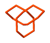
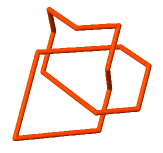
Figure 1: Lattice trefoils (of knot type $3_{1}^{+}$ in the standard knot tables [6]) in three dimensional cubic lattices. On the left a lattice trefoil is embedded in the simple cubic lattice. In the middle a lattice trefoil in the face-centered cubic lattice is illustrated, while the right panel is a realisation of a lattice trefoil in the body-centered cubic lattice.

A lattice polygon has length $n$ if it is composed of $n$ edges and $n$ vertices. The number of lattice polygons of length $n$ is the number of distinct polygons of length $n$, denoted by $p_{n}$. The function $p_{n}$ is the most basic combinatorial quantity associated with lattice polygons, and $\log p_{n}$ is a measure of the entropy of the lattice polygon at length $n$.

Determining $p_{n}$ in regular lattices is an old and difficult combinatorial problem [16]. Observe that $p_{2n+1}=0$ for $n\in{\mathbb{N}}$ in the SC lattice, and it known that the growth constant $\mu$ defined by the limit

$$\lim_{n\to\infty}p_{n}^{1/n}=\mu>0$$ (1)

exists and is finite in the SC lattice [16] if the limit is taken through even values of $n$. This result can be extended to other lattices, including the FCC and the BCC lattices, using the same basic approach in reference [16] (and by taking limits through even numbers in the BCC). In the hexagonal lattice it is known that $\mu=\sqrt{2+\sqrt{2}}$ [11].

In three dimensional lattices polygons are models of ring polymers. Knotted polygons are similarly a model of knotted ring polymers, see for example reference [13] on the importance of topology in the chemistry of ring polymers, and [9] on the occurrence of knotted conformations in DNA.

1.1 Knotted Polygons

Let $S^{1}$ be a circle. An embedding of $S^{1}$ into ${\mathbb{R}}^{3}$ is an injection $f:S^{1}\to{\mathbb{R}}^{3}$. We say that $f$ is tame if it contains no singular points, and a tame embedding is piecewise linear and finite if the image of $f$ is the union of line segments of finite length in ${\mathbb{R}}^{3}$. A tame piecewise linear embedding of $S^{1}$ into ${\mathbb{R}}^{3}$ is is also called a polygon.

Tame embeddings $S^{1}$ into ${\mathbb{R}}^{3}$ are tame knots, and the set of polygons compose a class of piecewise linear knots denoted by ${\cal K}_{p}$. If the class of all lattice polygons (for example, in a lattice ${\mathbb{L}}$) is denoted by ${\cal P}$, then ${\cal P}\subset{\cal K}_{p}$ so that each lattice polygon is also a tame and piecewise linear knot in ${\mathbb{R}}^{3}$. This defines the knot type $K$ of every polygon in a unique way. In particular, two polygons in ${\cal P}$ are equivalent as knots if and only if they are ambient isotopic as tame knots in ${\cal K}_{p}$.

Define $p_{n}(K)$ to be the number of lattice polygons in ${\mathbb{L}}$, of length $n$ and knot type $K$, counted modulo equivalence under translations in ${\mathbb{L}}$. Then $p_{n}(K)$ is the number of unrooted lattice polygons of length $n$ and knot type $K$. Observe that $p_{n}(K)=0$ if $n$ is odd, and hence, consider $p_{n}(K)$ to be a function on even numbers; $p_{n}(K):\,2{\mathbb{N}}\to{\mathbb{N}}$.

It follows that $p_{n}(0_{1})=0$ if $n<4$ and $p_{4}(0_{1})=3$ in the SC lattice where $0_{1}$ is the unknot (the simplest knot type). If $K\not=0_{1}$ is not the unknot, then in the SC lattice it is known that $p_{n}(K)=0$ if $n<24$ and that $p_{24}(K)>0$ [10]. In particular, $p_{24}(3_{1})=3328$ [43] while $p_{n}(K)=0$ if $K\not=0_{1}$ or $K\not=3_{1}$.

It is known that

$$\limsup_{n\to\infty}\left[p_{n}(K)\right]^{1/n}=\overline{\mu}_{K}<\mu$$ (2)

in the SC lattice; see reference [46]. If $K=0_{1}$ is the unknot, then it is known that

$$\lim_{n\to\infty}\left[p_{n}(0_{1})\right]^{1/n}=\mu_{0}<\mu$$ (3)

and it follows in addition that $\mu_{0}\leq\overline{\mu}_{K}<\mu$; see for example [22, 23]. There are substantial numerical evidence in the literature that $\mu_{0}=\overline{\mu}_{K}$ for all knot types $K$ (see reference [23] for a review, and references [41, 29, 33] for more on this). Overall, these results are strong evidence that the asymptotic behaviour of $p_{n}(K)$ is given to leading order to

$$p_{n}(K)\simeq C_{K}n^{\alpha_{0}+N_{K}-3}\mu_{0}^{n},$$ (4)

where $N_{K}$ is the number of prime components of knot type $K$, and $\alpha_{0}$ is the entropic exponent which is independent of knot type. The amplitude $C_{K}$ is dependent on the knot type $K$. In particular, simulations show that the amplitude ratio $\left[p_{n}(K)/p_{n}(L)\right]\to\left[C_{K}/C_{L}\right]\not=0$ if $N_{K}=N_{L}$ [41]; this strongly supports the proposed scaling in equation (4).

Growth constants for knotted polygons in the FCC and BCC in equations (2) and (3) have not been examined in the literature, but there is general agreement that the methods of proof in the SC lattice will demonstrate these same relations in the FCC and BCC. In particular, by concatenating SC lattice polygons as schematically illustrated in figure 2, it follows that

$$p_{n}(K)p_{m}(L)\leq 2\,p_{n+m}(K\#L)$$ (5)

where $K\#L$ is the connected sum of the knot types $K$ and $L$.

..............................................................................................................................................................................................................................................................................................................................................................................................................................................................................................................................................................................$\bullet$$\bullet$$\bullet$$\bullet$$\bullet$$\bullet$$\bullet$$\bullet$$\bullet$$\bullet$.....................................................................................................................................................................................................................................................................................................................................................................................................................................................................................................................................................................................................................................................................................................................................................................................................$\bullet$$\bullet$$\bullet$$\bullet$$\bullet$$\bullet$$\bullet$$\bullet$$\bullet$$\bullet$$\bullet$$\bullet$$\bullet$$\bullet$.........................................................

Figure 2: Concatenating polygons in the SC lattice. The top edge of the polygon on the left is defined at that edge with lexicographic most midpoint, and the bottom edge of the polygon on the right as that edge with lexicographic least midpoint. By translating, and rotating the polygon on the right until its bottom edge is parallel to the top edge of the polygon on the left, and translated one step in the $X$-direction, the two polygons can be concatenated into a single polygon by inserting the dotted polygon of length four between the two, as illustrated, and then deleting edges which are doubled up. If the polygon on the left has length $n$ and knot type $K$, then it can be chosen in $p_{n}(K)$ ways, and if the polygon on the right has length $m$ and knot type $L$, then it can be chosen in $p_{m}(L)/2$ ways, since its bottom edge much be parallel to the top edge of the polygon on the left. This shows that $p_{n}(K)p_{m}(L)\leq 2\,p_{n+m}(K\#L)$, since the concatenated polygon has length $n+m$ and knot type the connected sum $K\#L$ of the the knot types $K$ and $L$. This construction generalises in the obvious way to the FCC and BCC lattices.

Similar results are known in the FCC lattice: One has that $p_{n}(0_{1})=0$ if $n<3$, and $p_{3}(0_{1})=8$. Similarly, $p_{n}(3_{1})=0$ if $n<15$, while $p_{15}(3_{1})=64$. Observe that in the FCC lattice, $p_{n}(K)$ is a function on ${\mathbb{N}}$; $p_{n}(K):\,{\mathbb{N}}\to{\mathbb{N}}$. That is, there are polygons of odd length.

The construction in figure 2 generalises to the FCC lattice. In this case, the top vertex of the polygon is that vertex with lexicographic most coordinates. The top vertex $t$ is incident with two edges, and the top edge is that edge with midpoint with lexicographic most coordinates. The top edge of a FCC polygon is parallel to one of six possible directions, giving six different classes of polygons. One of these classes is the most numerous, containing at least $p_{n}(K)/6$ polygons and with top edge parallel to (say) direction $\beta$, if the polygons has length $n$ and knot type $K$.

Similarly, the bottom vertex and bottom edge of a FCC polygon of length $m$ and knot type $L$ can be identified, and there is a direction $\gamma$ such that the class of FCC polygons with bottom edge is parallel to $\gamma$ is the most numerous and is at least $p_{m}(L)/6$.

By choosing a polygon of knot type $K$, top vertex $t$ and length $n$ with top edge parallel to $\beta$, and a second polygon of length $m$, bottom vertex $b$, with bottom edge parallel to $\gamma$, these polygons can be concatenated similarly to the construction in figure 2 by inserting a polygon of length (say) $N+2$ between them. Accounting for the number of choices of the polygons on the left and right, and for the change in the number of edges, this shows that

$$p_{n}(K)p_{m}(L)\leq 36\,p_{n+m+N}(K\#L)$$ (6)

in the FCC, where $N$ is independent of $n$ and $m$ . The polygon of length $N+2$ is inserted to join the top and bottom edges of the respective polygons, since they may not be parallel a priori to the concatenation. Some reflection shows that the choice $N=2$ is sufficient in this case.

The relation in equation (6) shows that $[p_{n-N}/36]$ and $[p_{n-N}(0_{1})/36]$ are supermultiplicative functions in the FCC, and this proves existence of the limits $\lim_{n\to\infty}\left[p_{n}\right]^{1/n}=\mu$ and $\lim_{n\to\infty}\left[p_{n}(0_{1})\right]^{1/n}=\mu_{0}$ in the FCC [19]. In addition, with $\overline{\mu}_{K}$ defined in the FCC as in equation (2), it also follows from equation (6) that $\mu_{0_{1}}\leq\overline{\mu}_{K}\leq\mu$. That $\overline{\mu}_{K}<\mu$ would follow from a pattern theorem for polygons in the FCC (and it is widely expected that the methods in reference [36, 37] will prove a pattern theorem for polygons in the FCC).

In the BCC lattice one may verify that $p_{n}(0_{1})=0$ if $n<4$, and $p_{4}(0_{1})=12$. Similarly, $p_{n}(3_{1})=0$ if $n<18$, while $p_{18}(3_{1})=1584$. Observe that in the BCC lattice $p_{n}(K)$ is a function on even numbers; $p_{n}(K):\,2{\mathbb{N}}\to{\mathbb{N}}$, similar to the case in the SC lattice.

Finally, arguments similar to the above show that in the BCC lattice there exists an $N$ independent of $n$ and $m$ such that

$$p_{n}(K)p_{m}(L)\leq 16\,p_{n+m+N}(K\#L).$$ (7)

Thus, in the BCC one similarly expects that $\lim_{n\to\infty}\left[p_{n}\right]^{1/n}=\mu$ and $\lim_{n\to\infty}\left[p_{n}(0_{1})\right]^{1/n}=\mu_{0}$ exists in the BCC, and with $\overline{\mu}_{K}$ defined in the BCC as in equation (2), it also follows from equation (6) that $\mu_{0}\leq\overline{\mu}_{K}\leq\mu$. Similarly, a pattern theorem will show that $\overline{\mu}_{K}<\mu$. In the BCC one may choose $N=2$.

Generally, these results are consistent with the hypothesis that $\overline{\mu}_{K}=\mu_{0}$ in the BCC and FCC lattices, while the asymptotic form for $p_{n}(K)$ in equation (4) is expected to apply in these lattices as well. By computing amplitude ratios $\left[C_{K}/C_{L}\right]$ in reference [32] for a selection of knots, strong numerical evidence for equation (4) in the BCC and FCC were obtained.

1.2 Minimal Length Knots and the Lattice Edge Index

Given a knot type $K$ there exists an $n_{K}$ such that $p_{n_{K}}(K)>0$ but $p_{n}(K)=0$ for all $n<n_{K}$. The number $n_{K}$ is the minimal length of the knot type $K$ in the lattice [10, 27]. For example, if $K=3_{1}^{+}$ (a right-handed trefoil knot) then in the SC lattice it is known that $p_{24}(3_{1}^{+})=1664$ while $p_{n}(3_{1}^{+})=0$ for all $n<24$. Thus $n_{3_{1}^{+}}=24$ is the minimal length of (right-handed) trefoils in the SC lattice [45]. Observe that $n_{3_{1}^{+}}=n_{3_{1}^{-}}\,(=n_{3_{1}})$, and this is generally true for all knot types.

Similar results are not available in the BCC and FCC, although numerical simulations have shown that $n_{3_{1}^{+}}=18$ in the BCC and $n_{3_{1}^{+}}=15$ in the FCC [31, 32, 33].

The construction in figure 2 shows that

$$n_{K\#K}\leq 2\,n_{K}\,\,\hbox{and}\,\,n_{K\#L}\leq n_{K}+n_{L}$$ (8)

in the SC lattice. More generally, observe that for non-negative integers $p$,

$$n_{K^{p}}\leq p\,n_{K}.$$ (9)

This in particular shows that the minimal lattice edge index defined by

$$\inf_{p}\left[\frac{n_{K^{p}}}{p}\right]=\lim_{p\to\infty}\left[\frac{n_{K^{p}}}{p}\right]=\alpha_{K}$$ (10)

exists, and moreover, $\alpha_{K}\geq 4(b_{K}-1)$, where $b_{K}$ is the bridge number of the knot type $K$; see references [27, 20, 23] for details. Since $b_{K}\geq 2$ if $K\not=\emptyset$, it follows that $\alpha_{K}\geq 4$ for non-trivial knots types in the SC lattice. Observe that $\alpha_{0_{1}}=0$ and that it is known that $4\leq\alpha_{3_{1}^{+}}\leq 17$ [27, 20].

In the BCC and FCC lattices one may consult equations (6) and (7) to see that for non-negative integers,

$$n_{K^{p}\#K^{q}}\leq n_{K^{p}}+n_{K^{q}}+N.$$ (11)

Thus, $n_{K^{p}}+N$ is a subadditive function of $p$, and hence

$$\inf_{p}\left[\frac{n_{K^{p}}+N}{p}\right]=\lim_{p\to\infty}\left[\frac{n_{K^{p}}}{p}\right]=\alpha_{K}$$ (12)

exists [19]. Moreover, as in the SC lattice, one may present arguments similar to those in the proof of theorem 2 in reference [21] to see that $\alpha_{K}\geq 3(b_{K}-1)$ in the FCC and $\alpha_{K}\geq 2(b_{K}-1)$ in the BCC. Hence, if $K$ is not the unknot, then $\alpha_{K}\geq 3$ in the FCC and $\alpha_{K}\geq 2$ in the BCC.

We shall also work with the total number of distinct knot types $K$ with $n_{K}\leq n$, denoted by $Q_{n}$. It is known that $Q_{n}=1$ if $n<24$ in the SC lattice, and that $Q_{n}=3$ if $24\leq n<30$ [45], also in the SC lattice. $Q_{n}$ grows exponentially with $n$.

1.3 The Entropy of Minimal Length Knotted Polygons

If $n=n_{K}$, then $p_{n}(K)>0$ for a given knot type. The entropy of the knot type $K$ at minimal length is given by $\log p_{n}(K)$ when $n=n_{K}$. More generally, the entropy of lattice knots of minimal length and knot type $K$ can be studied by defining the density of the knot type $K$ at minimal length by

$${\cal P}_{K}=p_{n_{K}}(K).$$ (13)

Then one may verify that ${\cal P}_{\emptyset}=3$ in the SC lattice, and ${\cal P}_{\emptyset}=12$ in the BCC lattice while ${\cal P}_{\emptyset}=8$ in the FCC lattice.

It is also known that ${\cal P}_{3_{1}^{+}}=1664$ in the SC lattice [45]. Since $3_{1}$ is a chiral knot type, it follows that the total number of minimal length lattice polygons of knot type $3_{1}$ is given by ${\cal P}_{3_{1}}={\cal P}_{3_{1}^{+}}+{\cal P}_{3_{1}^{-}}=3328$.

Generally there does not appear to exist simple relations between ${\cal P}_{K}$ and ${\cal P}_{K^{m}}$. However, ${\cal P}_{K^{m}}$ should increase exponentially with $m$, since $n_{K^{m}}$ is bounded linearly with $m$ if $K$ is a non-trivial knot type [21]. Thus, the entropic index per knot component of the knot type $K$ can be defined by

$$\limsup_{m\to\infty}\left[\frac{\log{\cal P}_{K^{m}}}{m}\right]=\gamma_{K}.$$ (14)

Obviously, since ${\cal P}_{\emptyset^{m}}=4$ for all values of $m$, it follows that $\gamma_{\emptyset}=0$. Also, $\gamma_{K}\geq 0$ for all knot types $K$. Showing that $\gamma_{K}>0$ for all non-trivial knot types $K$ is an open question.

The collection of ${\cal P}_{K}$ minimal length lattice knots are partitioned in symmetry (or equivalence) classes by rotations and reflections (which compose the octahedral group, which is the symmetry group of the cubic lattices). Since the group has $24$ elements, each symmetry class may contain at most $24$ equivalent polygons. The total number of symmetry classes of minimal length lattice knots of type $K$ is denoted by ${\cal S}_{K}$. For example, in the SC lattice it is known that ${\cal S}_{0_{1}}=1$ and this class has $3$ minimal length lattice knots of length $4$. It has been shown that ${\cal S}_{3_{1}}=142$ in the SC, of which $137$ classes have $24$ members each and $5$ have $8$ members each [45].

1.4 The Mean Absolute Writhe of Minimal Length Knotted Polygons

The writhe of a closed curve is a geometric measure of its self-entanglement. It is defined as follows: The projection of a closed curve in ${\mathbb{R}}^{3}$ onto a geometric plane is regular if all multiple points in the projection are double points, and if projected arcs intersect transversely at each double point.

Intersections (referred to as “crossings”) in a regular projection are signed by the use of a right hand rule: The curve is oriented and the sign is assigned as illustrated in figure 3. The writhe of the projected curve is the sum of the signed crossings. The writhe of the space curve is the average writhe over all possible regular projections of the curve. For a lattice polygon $\omega$ this is defined by

$$W_{r}(\omega)=\frac{1}{4\pi}\int_{u\in S^{2}}W_{r}(\omega,u)$$ (15)

where $W_{r}(\omega,u)$ is the writhe of the projection along the unit vector $u$ (which takes values in the unit sphere $S^{2}$ – this is called the writhing number of the projection). This follows because almost all projections of $\omega$ are regular.

............................................................................................................................................................................................................................................................................................................................................................................................................................................................................................................................................................................................................................................................... ............................................................................................................................................................................................................................................................................................................................................................................................................................................................................................................................................................................................................................................................................

Figure 3: A negative crossing (left) and a positive crossing (right) of the intersections in a regular projections of a simple closed curved. The signs are assigned using a right hand rule.

The writhe of a closed curve was introduced by Fuller [14]. It was shown by Lacher and Sumners [38] that the writhe of a lattice curve is given by the average of the linking number of $\omega$ with its push-offs $\omega+\epsilon u$, for $u\in S^{2}$, and $\epsilon>0$ small. That is,

$$W_{r}(\omega)=\frac{1}{4\pi}\int_{u\in S^{2}}L_{k}(\omega,\omega+\epsilon u).$$ (16)

In the SC lattice, this simplifies to the average linking number of $\omega$ with four of its push-offs into non-antipodal octants:

$$W_{r}(\omega)=\frac{1}{4}\sum_{i=1}^{4}L_{k}(\omega,\omega+u_{i})$$ (17)

where, for example, one may take $u_{1}=(0.5,0.5,0.5)$, $u_{2}=(0.5,-0.5,0.5)$, $u_{3}=(-0.5,0.5,0.5)$ and $u_{4}=(-0.5,-0.5,0.5)$. This shows that $4\,W_{r}(K)$ is an integer.

The average writhe $\langle W_{r}(K)\rangle_{n}$ of polygons of knot type $K$ and length $n$ is defined by

$$\langle W_{r}(K)\rangle_{n}=\frac{1}{p_{n}(K)}\sum_{|\omega|=n}W_{r}(\omega)$$ (18)

where the sum is over all polygons of length $n$ and knot type $K$. If $K$ is an achiral knot, then $\langle W_{r}(K)\rangle_{n}=0$ for each value of $n$ [26].

The average absolute writhe $\langle\left|W_{r}(K)\right|\rangle_{n}$ of polygons of knot type $K$ and length $n$ is defined by

$$\langle\left|W_{r}(K)\right|\rangle_{n}=\frac{1}{p_{n}(K)}\sum_{|\omega|=n}\left|W_{r}(\omega)\right|$$ (19)

where the sum is over all polygons of length $n$ and knot type $K$.

The averaged writhe ${\cal W}_{K}$ and the average absolute writhe $|{\cal W}|_{K}$ of lattice knots of both minimal length and knot type $K$ are defined as the average and average absolute writhe of polygons of knot type $K$ and minimal length:

$${\cal W}_{K}=\langle W_{r}(K)\rangle_{n}{\hbox{\Large$|$}}_{n=n_{K}};\quad{\cal|W|}_{K}=\langle\left|W_{r}(K)\right|\rangle_{n}{\hbox{\Large$|$}}_{n=n_{K}}.$$ (20)

The writhe of polygons in the BCC and FCC lattices can also be determined by computing linking numbers between polygons and their push-offs [39]. Normally, the writhes in these lattices are related to the average writhing numbers of projections of the polygons onto planes normal to a set of given vectors.

The writhe of a polygon in the FCC lattice is normally an irrational number [15]. The prescription for determining the writhe of polygons in the FCC lattice can be found in reference [39] and is as follows: Put $\alpha=3{\,\hbox{arcsec}\,}3-\pi$ and $\beta=(\pi/2-\alpha)/3$. Then the writhe of a polygon $\omega$ is given by

$$W_{r}(\omega)=\frac{1}{2\pi}\left(\alpha\sum_{i=1}^{4}W_{r}(\omega,u_{i})+\beta\sum_{i=1}^{8}W_{r}(\omega,v_{i})\right)$$ (21)

where the vectors $u_{i}$ are defined by $u_{i}=(\pm 3/\sqrt{22},\pm 3/\sqrt{22},2/\sqrt{22})$ for all possible choices of the signs, and the vectors $v_{i}$ are defined by $v_{i}=(\pm\sqrt{5}/\sqrt{6},\pm 1/\sqrt{30},2/\sqrt{30})$, $(\pm 1/\sqrt{30},\pm\sqrt{5}/\sqrt{6},2/\sqrt{30})$, $(\pm 1/\sqrt{38},\pm 1/\sqrt{38},6/\sqrt{38})$ again for all possible choices of the signs. The writhing number $W_{r}(\omega,u_{i})$ of $\omega$ is defined as before as the sum of the signed crossings in the projected $\omega$ on a plane normal to $u_{i}$.

In the BCC lattice the writhe of a polygon $\omega$ can be computed by

$$W_{r}(\omega)=\frac{1}{12}\sum_{i=1}^{12}W_{r}(\omega,u_{i})$$ (22)

where the vectors $u_{i}$ are defined by $u_{i}=(\pm 1/\sqrt{10},3/\sqrt{10},0)$, $(\pm 1/\sqrt{10},0,3/\sqrt{10})$, $(0,\pm 1/\sqrt{10},3/\sqrt{10})$, $(0,3/\sqrt{10},\pm 1/\sqrt{10})$, $(3/\sqrt{10},\pm 1/\sqrt{10},0)$, $(3/\sqrt{10},0,\pm 1/\sqrt{10})$, for all possible choices of the signs.

By appealing to the Calugareanu and White formula $L_{k}=T_{w}+W_{r}$ [7, 50] for a ribbon, one can compute $W_{r}(\omega,u_{i})$ by creating a ribbon $(\omega,\omega+\epsilon u_{i})$ with boundaries $\omega$ and $\omega+\epsilon u_{i}$ (this is a push-off of $\omega$ by $\epsilon$ in the (constant) direction of $u_{i}$). Since the twist of this ribbon is zero, one has that $W_{r}(\omega,u_{i})=W_{r}(\omega+\epsilon u_{i},u_{i})=L_{k}(\omega,\omega+\epsilon u_{i})$, and the writhe can be computed by the linking number of the knot $W_{r}(\omega,u_{i})$ and its push-off $W_{r}(\omega,u_{i})+\epsilon u_{i}$.

Equation (22) shows that $12\,W_{r}(\omega)$ is an integer in the BCC lattice. Thus, the mean writhe of a finite collections of polygons in the BCC lattice is a rational number.

1.5 Curvature of Lattice Knots

The total curvature of an SC lattice polygon is equal to $\pi/2$ times the number of right angles between two edges. The average total curvature of minimal length polygons of knot type $K$ is denoted in units of $2\pi$ by ${\cal K}_{K}$ (that is, the average total curvature is $2\pi{\cal K}_{K}$). Obviously ${\cal K}_{0_{1}}=1$ in the SC lattice, since every minimal length unknotted polygon of length $4$ is a unit square of total curvature $2\pi$. For other knot types the total curvature of a polygon is an integer multiple of $\pi/2$, and the mean curvature is thus a rational number times $2\pi$. Hence, for a knot type $K$, the average curvature of minimal length length polygons of knot type $K$ is given by

$$\left\langle C_{K}\right\rangle=2\pi{\cal K}_{K}$$ (23)

where ${\cal K}_{K}$ is a rational number.

Similar definitions hold for polygons in the BCC and FCC. In each case the lattice curvature of a polygon is the sum of the complements of angles inscribed between successive edges.

In the FCC the curvature of a polygon is a summation over angles of sizes $0$, $\pi/3$ and $2\pi/3$. Hence $2\pi{\cal K}_{K}$ is a rational number similarly to the case in the SC. This gives a similar definition to equation (23) of ${\cal K}_{K}$ for minimal length lattice polygons of knot type $K$. Obviously, ${\cal K}_{0_{1}}=1$ in the FCC, since each minimal lattice polygon of knot type $0_{1}$ is an elementary equilateral triangle.

The situation is somewhat more complex in the BCC lattice. The curvature of a polygon is the sum over angles of sizes $\arccos(1/\sqrt{3})$, $\pi-\arccos(1/\sqrt{3})$ and $0$. This shows that the average curvature of minimal length polygons of knot type $K$ is of the generic form

$$\left\langle C_{K}\right\rangle={\cal B}_{K}\arccos(1/\sqrt{3})+2\pi{\cal K}_{K}$$ (24)

where ${\cal B}_{K}$ and ${\cal K}_{K}$ are rational numbers. By examining the $12$ minimal length unknotted polygons of length $4$ in the BCC, one can show that ${\cal B}_{0_{1}}=-2$ and ${\cal K}_{0_{1}}=3/2$.

The minimal lattice curvature ${\cal C}_{K}$ (as opposed to the average curvature) of SC lattice knots were examined in reference [28]. For example, it is known that ${\cal C}_{0_{1}}=2\pi$ while ${\cal C}_{3_{1}}=6\pi$ in the SC lattice [28]. Bounds on the minimal lattice curvature in the SC lattice can also be found in terms of the minimal crossing number $C_{K}$ or the bridge number $b_{K}$ of a knot. In particular, ${\cal C}_{K}\geq\max\left\{\left(3+\sqrt{9+8C_{K}}\right)\pi/4\,,\,3\pi b_{K}\right\}$. These bounds are in particular good enough to prove that ${\cal C}_{9_{47}}=9\pi$. A minimal lattice curvature index $\nu_{K}$ is also proven to exist in reference [28], in particular

$$\lim_{n\to\infty}\frac{{\cal C}_{K^{n}}}{n}=\nu_{K}$$ (25)

exists and ${\cal C}_{K^{n}}\geq n\nu_{K}$. It is known that $\nu_{0_{1}}=0$ but that $2\pi\leq\nu_{3_{1}}\leq 3\pi$ in the SC lattice, and one expect that $2\pi{\cal K}_{K^{n}}\geq{\cal C}_{K^{n}}\geq 2\pi n$ in the SC lattice. This shows that ${\cal K}_{K^{n}}$ increases at least as fast as $n$ in the SC lattice. For more details, see reference [28].

2 GAS Sampling of knotted polygons

Knotted polygons can be sampled by implementing the GAS algorithm [30]. The algorithm is implemented using a set of local elementary transitions (called “atmospheric moves” [29]) to sample along sequences of polygon conformations. The algorithm is a generalisation of the Rosenbluth algorithm [44], and is an approximate enumeration algorithm [24, 25].

The GAS algorithm can be implemented in the SC lattice on polygons of given knot type $K$ using the BFACF elementary moves [1, 2, 5] to implement the atmospheric moves [31, 32]. These elementary moves are illustrated in figure 3. This implementation is irreducible on classes of polygon of fixed knot type [35].

I:...............................................................................................................................................................................................................................................................$\bullet$$\bullet$$\bullet$$\bullet$$\bullet$$\bullet$...............................................................................................................................................................................................................................................................................................................................$\bullet$$\bullet$$\bullet$$\bullet$II:............................................................................................................................................................................................................$\bullet$$\bullet$$\bullet$$\bullet$$\bullet$..................................................................................................................................................................................................................................................................................................................................................................................$\bullet$$\bullet$$\bullet$$\bullet$$\bullet$

Figure 4: BFACF elementary moves on polygons in the cubic lattice. These (reversible) moves are of two types: Type I decreases or increases the length of the polygon by two edges, while Type II is a neutral move which maintains the length of the polygon. A move which increases the length of the polygon is a positive move, while negative moves decrease the length of the polygon.

The BFACF moves in figure 4 are either positive (increase the length of a polygon), neutral (leave the length unchanged) or negative (decrease the length of a polygon). These moves define the atmosphere of a polygon. The collection of possible positive moves constitutes the positive atmosphere of the polygon. Similarly, the collection of neutral moves composes the neutral atmosphere while the set of negative moves is the negative atmosphere of the polygon. The the size of an atmosphere of a polygon $\omega$ is the number of possible successful elementary moves that can be performed to change it into a different conformation. We denote the size of the positive atmosphere of a polygon $\omega$ by $a_{+}(\omega)$, of the neutral atmosphere by $a_{0}(\omega)$, and of the negative atmosphere by $a_{-}(\omega)$.

The GAS algorithm is implemented on cubic lattice polygons as follows (for more detail, see references [31, 32]). Let $\omega_{0}$ be a lattice polygon of knot type $K$, then sample along a sequence of polygons $\left\langle\omega_{0},\omega_{1},\omega_{2},\ldots\right\rangle$ by updating $\omega_{i}$ to $\omega_{i+1}$ using an atmospheric move.

Each atmospheric move is chosen uniformly from the collection of possible moves in the atmospheres. That is, if $\omega_{j}$ has length $\ell_{j}$ then the probabilities for positive, neutral and negative moves are given by

$$\hbox{Pr}(\hbox{$+$})\propto\beta_{\ell_{j}}a_{+}(\omega_{j}),\quad\hbox{Pr}(\hbox{$0$})\propto a_{0}(\omega_{j}),\quad\hbox{and}\,\hbox{Pr}(\hbox{$-$})\propto a_{-}(\omega_{j})$$ (26)

where the parameters $\beta_{\ell}$ were introduced in order to control the transition probabilities in the algorithm. It will be set in the simulation for “flat sampling”. That, it will be chosen approximately equal to the ratio of average sizes of the positive and negative atmospheres of polygons of length $\ell$: $\beta_{\ell}\approx\frac{{\left\langle a_{+}\right\rangle}_{\ell}}{{\left\langle a_{-}\right\rangle}_{\ell}}$. This choice makes the average probability of a positive atmospheric move roughly equal to the probability of a negative move at each value of $\ell$.

Ia:............................................................................................................................................................................................................................................................................................................................................................................$\bullet$$\bullet$$\bullet$$\bullet$$\bullet$$\bullet$...............................................................................................................................................................................................................................................................................................................................$\bullet$$\bullet$$\bullet$$\bullet$.......Ib:..................................................................................................................................................................................................................................................................................................................................................................................$\bullet$$\bullet$$\bullet$$\bullet$$\bullet$$\bullet$..........................................................................................................................................................................................................................................................................................................................................................................................................$\bullet$$\bullet$$\bullet$$\bullet$....................IIa:........................................................................................................................................................................................................................................................................................................$\bullet$$\bullet$$\bullet$$\bullet$$\bullet$............................................................................................................................................................................................................................................................................................................................................................................................................................$\bullet$$\bullet$$\bullet$$\bullet$$\bullet$.........................$\circ$......................................$\circ$IIb:...............................................................................................................................................................................................................................$\bullet$$\bullet$$\bullet$$\bullet$.....................................................................................................................................................................................................................................................................................................................................................................................................$\bullet$$\bullet$$\bullet$$\bullet$.......................................$\circ$.......................................$\circ$

Figure 5: Elementary moves on polygons in the BCC lattice. These (reversible) moves are of two types: Type I decreases or increases the length of the polygon by two edges, while Type II is a neutral move which maintains the length of the polygon.

Ia:................................................................................................................................................................................................................................................................................................................$\bullet$$\bullet$$\bullet$$\bullet$$\bullet$................................................................................................................................................................................................................................................................................................................................................................................$\bullet$$\bullet$$\bullet$$\bullet$.............................................................$\circ$

Figure 6: The Elementary move on polygons in the FCC lattice. This is the only class of elementary moves in this lattice, there are no neutral moves.

This sampling produces a sequence $\langle\omega_{j}\rangle$ of states and we assign a weight

$$W(\omega_{n})=\left[\frac{a_{-}(\omega_{0})+a_{0}(\omega_{0})+\beta_{\ell_{0}}a_{+}(\omega_{0})}{a_{-}(\omega_{n})+a_{0}(\omega_{n})+\beta_{\ell_{n}}a_{+}(\omega_{n})}\right]\times\prod_{j=0}^{n}\beta_{\ell_{j}}^{(\ell_{j}-\ell_{j+1})}.$$ (27)

to the state $\omega_{n}$. The GAS algorithm is an approximate enumeration algorithm in the sense that the ratio of average weights of polygons of lengths $n$ and $m$ tends to the ratio of numbers of such polygons. That is,

$$\frac{{\left\langle W\right\rangle}_{n}}{{\left\langle W\right\rangle}_{m}}=\frac{p_{n}(K)}{p_{m}(K)}.$$ (28)

The algorithm was coded using hash-coding such that updates of polygons and polygon atmospheres were done in $O(1)$ CPU time. This implementation was very efficient, enabling us to perform billions of iterations on knotted polygons in reasonable real time on desk top linux workstations. Minimal length polygons of each knot type were sieved from the data stream and hashed in a table to avoid duplicate discoveries. The lists of minimal length polygons were analysed separately by counting symmetry classes, and computing writhes and curvatures.

Implementation of GAS sampling in the FCC and BCC lattices proceeds similar to the implementation in the SC lattice. It is only required to define suitable atmospheric moves analogous to the SC lattice moves in figure 4, and to show that these moves are irreducible on classes of FCC or BCC lattice polygons of fixed knot types.

The BCC lattice has girth four, and local positive, neutral and negative atmospheric moves similar to the SC lattice moves in figure 4 can be defined in a very natural way. These are illustrated in figure 5. Observe that the conformations in this figure are not necessarily planar, in particular because minimal length lattice polygons in the BCC lattice are not necessarily planar. This collection of elementary moves is irreducible on classes of unrooted lattice polygons of fixed knot type $K$ in the BCC lattice [32, 33].

In the FCC lattice the generalisation of the BFACF elementary moves is a single class of positive atmospheric moves and their inverse, illustrated in figure 6. This elementary move (and its inverse) is irreducible on classes of unrooted lattice polygons of fixed knot type $K$ in the FCC lattice [32]. The implementation of this elementary move using the GAS algorithm is described in references [31, 32, 33].

3 Numerical Results

GAS algorithms for knotted polygons in the SC, BCC and FCC lattices were coded and run for polygons of lengths $n\leq M$ where $500\leq M\leq 700$, depending on the knot type (the larger values of $M$ were used for more complicated compound knots). In each simulation, up to 500 GAS sequences each of length $10^{7}$ states were realised with the purpose of counting and collecting minimal length polygons. In most cases the algorithm efficiently found minimal conformations in short real time, but a few knots proved problematic, and in particular compound knots. For example, knots types $(3_{1}^{+})^{5}$ and $(4_{1})^{3}$ required weeks of CPU time, while $(3_{1}^{+})^{2}(3_{1}^{-})^{2}$ proved to be beyond the memory capacity of our computers.

Generally, our simulations produced lists of symmetry classes of minimal length knotted polygons in the three lattices. Our data (lists of minimal length knotted polygons) are available at the website in reference [51].

3.1 Minimal Knots in the Simple Cubic Lattice

3.1.1 Minimal Length SC Lattice Knots:

The minimal lengths $n_{K}$ of prime knot types $K$ are displayed in table 1. We limited our simulations to prime knots up to eight crossings. In addition, a few knots with more than eight crossings were included in the table, including the first two knots in the knot tables to 12 crossings, as well as $9_{42}$ and $9_{47}$. The minimal lengths of some compound knots (up to eight crossings), as well as compound trefoils up to $(3_{1}^{+})^{6}$ and figure eights up to $(4_{1})^{6}$, were also examined, and data are displayed in table 2.

$n_{K}$	Prime Knot types
$4$	$0_{1}$
$24$	$3_{1}$
$30$	$4_{1}$
$34$	$5_{1}$
$36$	$5_{2}$
$40$	$6_{1}$, $6_{2}$, $6_{3}$
$42$	$8_{19}$
$44$	$7_{1}$, $7_{3}$, $7_{4}$, $7_{7}$, $8_{20}$
$46$	$7_{2}$, $7_{5}$, $7_{6}$, $8_{21}$
$48$	$8_{3}$, $8_{7}$, $9_{42}$
$50$	$8_{1}$, $8_{2}$, $8_{4}$, $8_{5}$, $8_{6}$, $8_{8}$, $8_{9}$, $8_{10}$, $8_{11}$, $8_{13}$, $8_{14}$, $8_{16}$, $9_{47}$
$52$	$8_{12}$, $8_{15}$, $8_{17}$, $8_{18}$
$54$	$9_{1}$
$56$	$9_{2}$
$60$	$10_{1}$, $10_{2}$
$64$	$11_{1}$
$66$	$11_{2}$
$70$	$12_{1}$, $12_{2}$

Table 1: Minimal Length of Prime Knots in the SC lattice.

The results in tables 1 and 2 confirms data previously obtained for minimal knots in the simple cubic lattice, see for example [21] and in particular reference [45] for extensive results on minimal length knotted SC polygons.

The number of different knot types with minimal length $n_{k}\leq n$ can be estimated and grows exponentially with $n$. In fact, if $Q_{n}$ is the number of different knot types with $n_{K}\leq n$, then $Q_{m}\geq Q_{n}$ if $m\geq n$. Obviously, $Q_{n}\leq p_{n}$, so that

$${\cal Q}=\limsup_{n\to\infty}Q_{n}^{1/n}\leq\lim_{n\to\infty}p_{n}^{1/n}=\mu$$ (29)

by equation (1).

On the other hand, suppose that $N>0$ prime knot types (different from the unknot) can be tied in polygons of length $m$ (that is $Q_{m}\geq N$). Then by concatenating $k$ polygons of different prime knot types as in figure 2, it follows that $Q_{Nm}\geq\sum_{k=0}^{N}\left({{N}\atop{k}}\right)=2^{N}$. In other words

$$Q_{n}\geq 2^{n/m}.$$ (30)

if $n=Nm$ where $N$ is the number of non-trivial prime knot types that can be tied in a polygon of length $n$. For example, if $m=28$, then $N=1$, and thus $Q_{28}\geq 2$. Taking $n\to\infty$ implies that $N\to\infty$ as well so that $\liminf_{n\to\infty}Q_{n}^{1/n}\geq 1$.

In other words, $1\leq{\cal Q}\leq\mu$.

Thence, one may estimate $Q_{n}^{1/n}$, and increasing $n$ in $Q_{n}^{1/n}$ should give increasingly better estimates of ${\cal Q}$. In addition, if $Q_{n}^{1/n}$ approaches a limit bigger than one, then ${\cal Q}>1$ and the number of different knot types that can be tied in a polygon of length $n$ increases exponentially with $n$.

By examining the data in tables 1 and 2, one observes that $Q_{30}=4$ so that ${\cal Q}\approx 4^{1/30}\approx 1.0472\ldots$. Increasing $n$ to $40$ gives $Q_{40}=16$, so that ${\cal Q}\approx 1.07177\ldots$. If $n=50$, then $Q_{50}\geq 74$, hence ${\cal Q}\approx 1.08989\ldots$. These approximate estimates of ${\cal Q}$ increases systematically, suggesting the estimates are lower bounds, and that ${\cal Q}>1$.

The number of distinct knot types with $n_{K}=n$ is $\overline{Q}_{n}=Q_{n}-Q_{n-1}$, and since $Q_{n}\geq Q_{n-1}$ and $Q_{n}={\cal Q}^{n+o(n)}$, it follows that $\overline{Q}_{n}=0$ if $n$ is odd, and $\overline{Q}_{n}={\cal Q}^{n+o(n)}$ for even values of $n$.

There appears to be several cases of regularity amongst the minimal lengths of knot types in tables 1. The sequence of $(N,2)$-torus knots with $N\geq 3$ (these are the knots $\{3_{1},5_{1},7_{1},9_{1},11_{1}\}$) increases in steps of $10$ starting in $24$. Similarly, the sequence of twist knots $\{4_{1},6_{1},8_{1},10_{1},12_{1}\}$ increments in $10$ starting in $30$, as do the sequence of twist knots $\{5_{2},7_{2},9_{2},11_{2}\}$, but starting in $36$. The sequence $\{4_{1},6_{2},8_{2},10_{2},12_{2}\}$ also increments in $10$, starting at $30$ as well. A discussion of these patterns can be found in reference [21] (see figure 3 therein). There are no proofs that these patterns will persist indefinitely.

$n_{K}$	Compound Knot Types
$40$	$(3_{1}^{+})^{2}$, $(3_{1}^{+})(3_{1}^{-})$
$46$	$(3_{1}^{+})(4_{1})$
$50$	$(5_{1}^{+})(3_{1}^{+})$, $(5_{1}^{+})(3_{1}^{-})$, $(5_{2}^{+})(3_{1}^{-})$
$52$	$(4_{1})^{2}$, $(5_{2}^{+})(3_{1}^{+})$
$56$	$(3_{1}^{+})^{3}$, $(3_{1}^{+})^{2}(3_{1}^{-})$
$72$	$(3_{1}^{+})^{4}$
$74$	$(4_{1}^{+})^{3}$
$88$	$(3_{1}^{+})^{5}$
$96$	$(4_{1})^{4}$
$104$	$(3_{1}^{+})^{6}$
$118$	$(4_{1})^{5}$
$140$	$(4_{1})^{6}$

Table 2: Minimal Length of Compound Knots in the SC lattice.

In table 2 the estimated minimal lengths $n_{K}$ of a few compounded knots are given. These data similarly exhibit some level of regularity. For example, the family of compounded positive trefoils $\left\{(3_{1}^{+})^{n}\right\}$ increases in steps of $16$ starting in $24$. From these data, one may bound the minimal lattice edge index of positive trefoils (defined in equation (10)). In particular, $\alpha_{K}\leq n_{K^{p}}/p$, and if $K=3_{1}^{+}$ and $p=6$, then it follows that $\alpha_{3_{1}^{+}}\leq 17\frac{1}{3}$. This does not improve on the upper bound given in references [27] and [20], but if the increment of $16$ persists, then if $p=10$ one would obtain $\alpha_{3_{1}^{+}}\leq 16\frac{4}{5}<17$. Preliminary calculations indicated that finding the minimal edge number for $(3_{1}^{+})^{10}$ would be a difficult simulation, and this was not pursued. At this point, the argument illustrated in figure 4 in reference [21] proves that $\alpha_{3_{1}^{+}}\leq 17$, and the data above suggest that $\alpha_{3_{1}}=24+16n$ for $n\leq 6$. If this pattern persists, then $\alpha_{K}$ would be equal to $16$, but there is no firm theoretical argument which validates this expectation.

Similar observations apply to the family of compounded figure eight knots $\left\{(4_{1})^{n}\right\}$. The minimal edge numbers for $n\leq 6$ are displayed in table 2 and increments by $22$ such that $\alpha_{4_{1}}=30+22n$ for $n\leq 6$. This suggest that $\alpha_{4_{1}}=22$, but the best upper bound from the data in table 2 is $23\frac{2}{3}$.

Knot	Simple Cubic Lattice
	$n_{K}$	${\cal P}_{K}$	${\cal S}_{K}$		${\cal W}_{K}$	${\cal|W|}_{K}$	${\cal K}_{K}$
$0_{1}$	4	3	1	$3^{1}$	0	0	1
$3_{1}$	24	3328	142	$24^{137}8^{5}$	$3\frac{735}{1664}$	$3\frac{735}{1664}$	$3\frac{801}{1664}$
$4_{1}$	30	3648	152	$24^{152}$	$0$	$\frac{33}{152}$	$4\frac{1}{152}$
$5_{1}$	34	6672	278	$24^{278}$	$6\frac{127}{556}$	$6\frac{127}{556}$	$4\frac{459}{556}$
$5_{2}$	36	114912	4788	$24^{4788}$	$4\frac{5057}{9576}$	$4\frac{5057}{9576}$	$5\frac{61}{9576}$
$6_{1}$	40	6144	258	$24^{254}12^{4}$	$1\frac{49}{512}$	$1\frac{49}{512}$	$5\frac{223}{512}$
$6_{2}$	40	32832	1368	$24^{1368}$	$2\frac{1079}{1368}$	$2\frac{1079}{1368}$	$5\frac{65}{456}$
$6_{3}$	40	3552	148	$24^{148}$	$0$	$\frac{29}{148}$	$4\frac{36}{37}$
$7_{1}$	44	33960	1415	$24^{1415}$	$9\frac{61}{283}$	$9\frac{61}{283}$	$6\frac{322}{1415}$
$7_{2}$	46	336360	14016	$24^{14014}12^{2}$	$5\frac{10539}{14015}$	$5\frac{10539}{14015}$	$6\frac{811}{28030}$
$7_{3}$	44	480	20	$24^{20}$	$7\frac{19}{40}$	$7\frac{19}{40}$	$5\frac{31}{40}$
$7_{4}$	44	168	7	$24^{7}$	$5\frac{4}{7}$	$5\frac{4}{7}$	$5\frac{2}{7}$
$7_{5}$	46	9456	394	$24^{394}$	$7\frac{107}{394}$	$7\frac{107}{394}$	$6\frac{83}{394}$
$7_{6}$	46	34032	1418	$24^{1418}$	$3\frac{625}{1418}$	$3\frac{625}{1418}$	$5\frac{614}{709}$
$7_{7}$	44	504	21	$24^{21}$	$\frac{43}{84}$	$\frac{43}{84}$	$5\frac{1}{12}$
$8_{1}$	50	23736	990	$24^{988}12^{2}$	$2\frac{813}{1978}$	$2\frac{813}{1978}$	$6\frac{514}{989}$
$8_{2}$	50	91680	3820	$24^{3820}$	$5\frac{2081}{3820}$	$5\frac{2081}{3820}$	$6\frac{1259}{3820}$
$8_{3}$	48	12	1	$12^{1}$	$0$	$0$	$5\frac{91}{97}$
$8_{4}$	50	47856	1994	$24^{1994}$	$1\frac{2613}{3988}$	$1\frac{2613}{3988}$	$6\frac{1675}{3988}$
$8_{5}$	50	1152	48	$24^{48}$	$5\frac{5}{8}$	$5\frac{5}{8}$	$6\frac{5}{24}$
$8_{6}$	50	11040	460	$24^{460}$	$4\frac{7}{920}$	$4\frac{7}{920}$	$6\frac{273}{920}$
$8_{7}$	48	48	2	$24^{2}$	$2\frac{3}{4}$	$2\frac{3}{4}$	$5\frac{3}{4}$
$8_{8}$	50	3120	130	$24^{130}$	$1\frac{21}{260}$	$1\frac{21}{260}$	$6\frac{89}{260}$
$8_{9}$	50	35280	1470	$24^{1470}$	$0$	$\frac{527}{2940}$	$6\frac{307}{980}$
$8_{10}$	50	1680	70	$24^{70}$	$3\frac{1}{140}$	$3\frac{1}{140}$	$5\frac{121}{140}$
$8_{11}$	50	192	8	$24^{8}$	$4\frac{1}{8}$	$4\frac{1}{8}$	$6\frac{3}{8}$
$8_{12}$	52	2592	108	$24^{108}$	$\frac{71}{216}$	$\frac{71}{216}$	$6\frac{187}{216}$
$8_{13}$	50	26112	1088	$24^{1088}$	$1\frac{399}{2176}$	$1\frac{399}{2176}$	$5\frac{2099}{2176}$
$8_{14}$	50	720	30	$24^{30}$	$3\frac{59}{60}$	$3\frac{59}{60}$	$6\frac{29}{60}$
$8_{15}$	52	80208	3342	$24^{3342}$	$7\frac{2957}{3342}$	$7\frac{2957}{3342}$	$6\frac{549}{1114}$
$8_{16}$	50	96	4	$24^{4}$	$2\frac{5}{8}$	$2\frac{5}{8}$	$5\frac{7}{8}$
$8_{17}$	52	53184	2216	$24^{2216}$	$0$	$\frac{1099}{4432}$	$6\frac{321}{4432}$
$8_{18}$	52	3552	148	$24^{148}$	$0$	$\frac{10}{37}$	$5\frac{71}{148}$
$8_{19}$	42	13992	592	$24^{574}12^{18}$	$8\frac{885}{1166}$	$8\frac{885}{1166}$	$5\frac{267}{583}$
$8_{20}$	44	240	10	$24^{10}$	$2\frac{1}{10}$	$2\frac{1}{10}$	$4\frac{9}{10}$
$8_{21}$	46	56040	2335	$24^{2335}$	$4\frac{2499}{4670}$	$4\frac{2499}{4670}$	$5\frac{373}{467}$
$9_{1}$	54	345960	14417	$24^{14414}8^{3}$	$12\frac{283}{4805}$	$12\frac{283}{4805}$	$7\frac{5763}{9610}$
$9_{2}$	56	3281304	136721	$24^{136721}$	$6\frac{105057}{136721}$	$6\frac{105057}{136721}$	$7\frac{96676}{136721}$
$9_{42}$	48	27744	1156	$24^{1156}$	$1\frac{953}{2312}$	$1\frac{953}{2312}$	$5\frac{1939}{2312}$
$9_{47}$	50	13680	570	$24^{570}$	$2\frac{4}{5}$	$2\frac{4}{5}$	$5\frac{47}{95}$
$10_{1}$	60	462576	19298	$24^{19250}12^{48}$	$3\frac{12507}{38548}$	$3\frac{12507}{38548}$	$8\frac{5341}{38548}$
$10_{2}$	60	871296	36304	$24^{36304}$	$8\frac{42761}{72608}$	$8\frac{42761}{72608}$	$7\frac{56813}{72608}$

Table 3: Data on prime knot types in the SC Lattice.

3.1.2 Entropy of minimal lattice knots in the SC lattice:

Minimal length lattice knots were sieved from the data stream, then classified and stored during the simulations, which was allowed to continue until all, or almost all, minimal length lattice were discovered. In several cases a simulation was repeated in order to check the results. We are very sure of our data if ${\cal P}_{K}\lesssim 1000$, reasonable certain if $1000\lesssim{\cal P}_{K}\lesssim 10000$, less certain if $10000\lesssim{\cal P}_{K}\lesssim 100000$, and we consider the stated value of ${\cal P}_{K}$ to be only a lower bound if ${\cal P}_{K}\gtrsim 100000$ in table 3.

Data on entropy, lattice writhe and lattice curvature, were collected on prime knot types up to eight crossings, and also the knot types $9_{1}$, $9_{1}$, $9_{42}$, $9_{47}$, $10_{1}$ and $10_{2}$. The SC lattice data are displayed in table 3. As before, the minimal length of a knot type $K$ is denoted by $n_{K}$, and ${\cal P}_{K}=c_{n_{K}}(K)$ is the total number of minimal length SC lattice knots of length $n_{K}$. For example, there are $3328$ minimal length trefoils (of both chiralities) of length $n_{3_{1}}=24$. Since $3_{1}$ is chiral, ${\cal P}_{3_{1}^{+}}=3328/2=1664$.

The unknot has minimal length $4$, which is a unit square polygon in a symmetry class of $3$ members which are equivalent under lattice symmetries. The $3328$ minimal lattice trefoils are similarly partitioned into $142$ symmetry classes, of which $137$ classes has $24$ members and $5$ classes has $8$ members each. These partitionings into symmetry classes are denoted by $3^{1}$ for the unknot, and $24^{137}8^{5}$ for lattice polygons of knot type $3_{1}$ (of both chiralities) or $12^{137}4^{5}$ for lattice polygons of (say) right-handed knot type $3_{1}^{+}$.

Entropy per unit length of minimal polygons of knot type $K$ is defined by

$${\cal E}_{K}=\frac{\log{\cal P}_{K}}{n_{K}}.$$ (31)

This is a measure of the tightness of the minimal knot. If ${\cal E}_{K}$ is small, then there are few conformations that the minimal knot can explore, and such a knot is tightly embedded in the lattice (and its edges are relatively immobile). If ${\cal E}_{K}$, on the other hand, is large, then there are a relatively large conformational space which the edges may explore, and such a knot type is said to be loosely embedded.

The unknot has ${\cal E}_{0_{1}}=(\log 3)/4=0.27467\ldots$, which will be small compared to other knot types, and is thus tightly embedded.

The entropy per unit length of the (right-handed) trefoils is ${\cal E}_{3_{1}^{+}}=(\log 1664)/24=0.3090\ldots$, and it appears that the edges in these tight embeddings are similarly constrained to those in the unknot. Edges in the (achiral) knot $4_{1}$ has ${\cal E}_{4_{1}}=(\log 3648)/30=0.2733\ldots<{\cal E}_{3_{1}^{+}}$, and are more constrained than those in the trefoil. Similarly, for five crossing knots one finds that ${\cal E}_{5_{1}^{+}}=0.2386\ldots$ while ${\cal E}_{5_{2}^{+}}=0.3223\ldots$.

The entropy per unit length seems to converge in families of knot types. For example in the $(N,2)$-torus knot family $\{3_{1}^{+},5_{1}^{+},7_{1}^{+},9_{1}^{+}\}$ one gets $\{0.3090,0.2386,0.2214,0.2234\}$ to four digits accuracy. Similarly, the family of twist knots $\{3_{1}^{+},5_{2}^{+},7_{2}^{+},9_{2}^{+}\}$ gives $\{0.3090,0.3044,0.2616,0.2555\}$, again to four digits. Similar patterns are observed for the families $\{6_{1}^{+},8_{1}^{+},10_{1}^{+}\}$ ($\{0.2008,0.1876,0.2059\}$), and $\{6_{2}^{+},8_{2}^{+},10_{2}^{+}\}$ ($\{0.2427,0.2147,0.2164\}$). Further extensions of the estimates of ${\cal P}_{K}$ for more complicated knots would be necessary to test these patterns, but the scope of such simulations are beyond our available computing resources.

Finally, there are some knots with very low entropy per unit length. These include $7_{3}^{+}$ ($0.1246$), $7_{4}^{+}$ ($0.1007$), $7_{7}^{+}$ ($0.1257$), $8_{3}$ ($0.08065$), $8_{7}^{+}$ ($0.06621$), $8_{11}^{+}$ ($0.09129$), $8_{16}^{+}$ ($0.07742$) and $8_{20}^{+}$ ($0.1088$). These knots are tightly embedded in the SC lattice in their minimal conformations, with very little entropy per edge available.

The distribution of minimal knotted polygons in symmetry classes in table 3 shows that most minimal knotted polygons are not symmetric with respect to elements of the octahedral group, and thus fall into classes of $24$ distinct polygons. Classes with fewer elements, (for example $12$ or $8$), has symmetric embeddings of the embedded polygons. Such symmetric embeddings are the exception rather than the rule in table 3: For example, amongst the listed prime knot types in that table, only eight types admit to a symmetric embedding.

3.1.3 The Lattice Writhe and Curvature:

The average writhe ${\cal W}_{K}$, the average absolute writhe $|{\cal W}|_{K}$ and the average curvature ${\cal K}_{K}$ (in units of $2\pi$) of minimal length polygons are displayed in table 3. The results are given as rational numbers, since these numbers can be determined exactly from the data. Observe that the writhe of simple cubic lattice polygons are known to be rational numbers [38, 26, 34], hence the average over finite sets of polygons will also be rational. In addition, the average writhe ${\cal W}_{K}$ is non-negative in table 3 since the right handed knot was in each case used in the simulation.

In most cases in table 3 it was observed that $|{\cal W}_{K}|=|{\cal W}|_{K}$, with the exception of some achiral knots, which have $|{\cal W}|_{K}>0$ while ${\cal W}_{K}=0$. The average absolute writhe was zero in only two cases, namely the unknot and the knot $8_{3}$. Generally, the average and absolute average writhe of achiral knots are not equal, but the unknot and $8_{3}$ are exceptions to this rule.

Knot	Simple Cubic Lattice
	$n$	${\cal P}_{K}$	${\cal S}_{K}$		${\cal W}_{K}$	${\cal|W|}_{K}$	${\cal K}_{K}$
$3_{1}$	24	3328	142	$24^{137}8^{5}$	$3\frac{735}{1664}$	$3\frac{735}{1664}$	$3\frac{801}{1664}$
	26	281208	11721	$24^{11713}12^{8}$	$3\frac{10773}{23434}$	$3\frac{10773}{23434}$	$3\frac{23017}{23434}$
	28	14398776	599949	$24^{599949}$	$3\frac{40144}{85707}$	$3\frac{40144}{85707}$	$4\frac{267364}{599949}$

Table 4: SC Lattice Trefoils of lengths $24$, $26$ and $26$.

It is known that achiral knots have zero average writhe [34], and so ${\cal W}_{K}=0$ if the knot type $K$ is achiral. For example, ${\cal W}_{3_{1}}=3\frac{735}{1664}\approx 3.4417\ldots$ (for right handed trefoils), and hence $3_{1}$ is a chiral knot type. This numerical estimate for ${\cal W}_{3_{1}}$ is consistent with the results of simulations done elsewhere [26, 34], and it appears that ${\cal W}_{3_{1}}$ is only weakly dependent on the length of the polygons. For example, in table 4 the average and average absolute writhe of polygons with knot type $3_{1}^{+}$ and lengths $24$, $26$ and $28$ are listed. Observe that while ${\cal W}_{3_{1}}$ and $|{\cal W}|_{K}$ do change with increasing $n$, it is also so that the change is small, that is, it changes from $3.44170\ldots$ for $n=24$ to $3.45971\ldots$ to $3.46848\ldots$ as $n$ increments from $n=24$ to $n=28$. These numerical values are close to the estimates of average writhes made elsewhere in the literature for polygons of significant increased length, and the average writhe seems to cluster about the estimate $3.44\ldots$ in those simulations [26, 4, 43].

Generally, the average and average absolute writhe increases with crossing number in table (3). However, in each class of knot types of crossing number $C>3$ there are knot types with small average absolute writhe (and thus with small average writhe). For example, amongst the class of knot types on eight crossings, there are achiral knots with zero absolute writhe ($8_{3}$), as well as chiral knot types with average absolute writhe small compared to the average absolute writhe of (say) $8_{1}$. For example, the average absolute writhe of $8_{18}$ is $10/37$. The obvious question following from this observation is on the occurrence of such knot types: Since there are chiral knot types with average absolute writhe less than $1$ for knots on $4$, $6$, $7$ and $8$ crossings in table 3, would such chiral knot types exist for all knot types on $C\geq 6$ crossings?

The curvature of a cubic lattice polygon is a multiple of $\pi/2$, and hence the average curvature will similarly be a rational number times $2\pi$: That is, $\left\langle C_{K}\right\rangle=2\pi{\cal K}_{K}$ where $\left\langle C_{K}\right\rangle$ is the average curvature of minimal length polygons of knot type $K$ and ${\cal K}_{K}$ is the rational number displayed in the last column of table 3. For example, the average curvature of minimal length lattice trefoils is $6\left[\frac{801}{832}\right]\pi\approx 6.96274\pi$.

The variability in ${\cal K}_{K}$ is less than that observed for the writhe ${\cal W}_{K}$ in classes of knot types of given crossing number in table 3. Generally, increasing the crossing number increases the minimal length of the knot type, with a similar increase in the number of right angles in the polygon. This increase is reflected in the increase of ${\cal K}_{K}$ with increasing $n_{K}$.

The ratio ${\cal K}_{K}/n_{K}$ stabilizes quickly in families of knot types. For example, for $(N,2)$-torus knots, this ratio decreases with increasing $n_{K}$ as $\{0.25,0.141,0.142,0.141\}$ as $K$ increases along $\{3_{1},5_{1},7_{1},9_{1}\}$. Similar patterns can be determined for other families of knot types. For example, for the twist knots $K=\{4_{1},6_{1},8_{1},10_{1}\}$, the ratio is also stable, but a little bit lower: $\{0.145,0.136,0.131,0.136\}$.

Finally, it was observed before equation (25) that the minimal curvature of a lattice knot in the SC lattice, ${\cal C}_{K}$, can be defined and that ${\cal C}_{0_{1}}=2\pi$, ${\cal C}_{3_{1}}=6\pi$ and ${\cal C}_{9_{47}}=9\pi$. The average curvatures in table 3 exceeds these lower bounds in general, with equality only for the unknot: For example, ${\cal K}_{3_{1}}=6\frac{801}{832}\pi$ and ${\cal K}_{9_{47}}=10\frac{94}{95}\pi$. However, in each of these knot types there are realizations of polygons with both minimal length and minimal curvature.

3.2 Minimal Knots in the Face Centered Cubic Lattice

$n_{K}$	Prime Knot types
$3$	$0_{1}$
$15$	$3_{1}$
$20$	$4_{1}$
$22$	$5_{1}$
$23$	$5_{2}$
$27$	$6_{1}$, $6_{2}$
$28$	$6_{3}$, $8_{19}$
$29$	$7_{1}$
$30$	$7_{2}$, $7_{3}$, $7_{4}$, $8_{20}$
$31$	$7_{5}$, $7_{6}$, $7_{7}$, $8_{21}$
$32$	$9_{42}$
$34$	$8_{1}$, $8_{2}$, $8_{3}$, $8_{4}$, $8_{5}$, $8_{6}$, $8_{7}$, $8_{8}$, $8_{9}$, $8_{10}$
$35$	$8_{11}$, $8_{12}$, $8_{13}$, $8_{14}$, $8_{15}$, $8_{16}$, $8_{17}$, $9_{1}$, $9_{47}$
$36$	$8_{18}$
$37$	$9_{2}$
$40$	$10_{1}$, $10_{2}$

Table 5: Minimal Length of knot types in the FCC lattice.

3.2.1 Minimal Length FCC Lattice Knots:

The minimal lengths $n_{K}$ of prime knot types $K$ in the FCC are displayed in table 5. Prime knots types up to eight crossings are included, together with a few knots with nine crossings, as well as the knots $10_{1}$ and $10_{2}$. In general the pattern of data in table 5 are similar to the results in the SC lattice in table 1. Observe that while the knot type $6_{*}$ can be tied with $40$ edges in the SC lattice, in the FCC lattice $6_{1}$ and $6_{2}$ can be tied with fewer edges than $6_{3}$. Similarly, the knot $7_{1}$ can be tied with fewer edges than other seven crossing knots in the FCC lattice, but not in the SC lattice. There are other similar minor changes in the ordering of the knot types in table 5 compared to the SC lattice data in table 1.

Similar to the argument in the SC lattice, one may define $Q_{n}$ to be the number of different knot types with $n_{K}\leq n$ in the FCC lattice. It follows that $Q_{n}\leq p_{n}$, so that

$${\cal Q}=\limsup_{n\to\infty}Q_{n}^{1/n}\leq\lim_{n\to\infty}p_{n}^{1/n}=\mu$$ (32)

by equation (1).

By counting the number of distinct knot types with $n_{K}\leq n$ in tables 5 one may estimate ${\cal Q}$ by computing $Q_{n}^{1/n}$: Observe that $Q_{3}=1$ and $Q_{15}=2$, this shows that ${\cal Q}\approx 1.041\ldots$. By increasing $n$, one finds that $Q_{35}\geq 37$, and this gives the estimate ${\cal Q}\approx 1.10550\ldots$. This is larger than the estimate of ${\cal Q}$ in the SC lattice, and may be some evidence that the exponential rate of growth of $Q_{n}$ in the FCC lattice is strictly larger than in the SC lattice: That is, ${\cal Q}_{FCC}>{\cal Q}_{SC}$.

Similar to the case in the SC, the number of distinct knot types with $n_{K}=n$ is $\overline{Q}_{n}=Q_{n}-Q_{n-1}$, and since $Q_{n}\geq Q_{n-1}$ and $Q_{n}={\cal Q}^{n+o(n)}$, it follows that $\overline{Q}_{n}={\cal Q}^{n+o(n)}$.

There are several cases of (semi)-regularity amongst the minimal lengths of knot types in tables 5. $(N,2)$-torus knots with $3\leq N\leq 5$ (these are the knots $\{3_{1},5_{1},7_{1}\}$) have increases in steps of $7$ starting in $15$. This pattern, however, fails for the next member in this sequence, since $n_{9_{1}}=35$, an increment of $6$ from $7_{1}$. Similar observations are true of the sequence of twist knots. The sequence $\{4_{1},6_{1},8_{1}\}$ has increments of $7$ starting in $20$, but this breaks down for $10_{1}$, which increments by $6$ over $n_{8_{1}}$. The first three members of the sequence of twist knots $\{5_{2},7_{2},9_{2}\}$ similarly have increments in steps of $7$, and if the patterns above applies in this case as well, then this should break down as well. Observe that these results are different from the results in the SC lattice. In that case, the patterns persisted for the knots examined, but in the FCC lattice the patterns break down fairly quickly.

Knot	Face Centered Cubic Lattice
	$n_{K}$	${\cal P}_{K}$	${\cal S}_{K}$		${\cal W}_{K}$	${\cal|W|}_{K}$	${\cal K}_{K}$
$0_{1}$	3	8	1	$8^{1}$	0	0	1
$3_{1}$	15	64	4	$24^{2}8^{2}$	$3.3245203$	$3.3245203$	$2\frac{3}{4}$
$4_{1}$	20	2796	130	$24^{106}12^{18}6^{6}$	$0$	$0.0649554$	$3\frac{175}{699}$
$5_{1}$	22	96	4	$24^{4}$	$6.04086733$	$6.04086733$	$3\frac{1}{2}$
$5_{2}$	23	768	32	$24^{32}$	$4.58773994$	$4.58773994$	$3\frac{3}{4}$
$6_{1}$	27	19008	792	$24^{792}$	$1.30062599$	$1.30062599$	$4\frac{449}{1188}$
$6_{2}$	27	5040	210	$24^{210}$	$2.68566969$	$2.68566969$	$4\frac{199}{630}$
$6_{3}$	28	102720	4280	$24^{4280}$	$0$	$0.10145467$	$4\frac{11519}{25680}$
$7_{1}$	29	4080	170	$24^{170}$	$8.83566369$	$8.83566369$	$4\frac{919}{1020}$
$7_{2}$	30	4128	172	$24^{172}$	$5.94373229$	$5.94373229$	$4\frac{37}{43}$
$7_{3}$	30	960	40	$24^{40}$	$7.30408669$	$7.30408669$	$4\frac{3}{5}$
$7_{4}$	30	96	4	$24^{4}$	$6.17547989$	$6.17547989$	$4\frac{5}{6}$
$7_{5}$	31	27456	1144	$24^{1144}$	$7.31767838$	$7.31767838$	$4\frac{853}{858}$
$7_{6}$	31	4896	204	$24^{204}$	$3.29853635$	$3.29853635$	$5\frac{2}{17}$
$7_{7}$	32	1296	54	$24^{54}$	$0.66279311$	$0.66279311$	$5\frac{35}{162}$
$8_{1}$	34	447816	18696	$24^{18622}12^{74}$	$2.51971823$	$2.51971823$	$5\frac{11155}{18659}$
$8_{2}$	34	116016	4834	$24^{4834}$	$5.39777682$	$5.39777682$	$5\frac{7991}{14502}$
$8_{3}$	34	19200	800	$24^{800}$	$0$	$0.06471143$	$5\frac{73}{240}$
$8_{4}$	34	41088	1712	$24^{1712}$	$1.39528958$	$1.39528958$	$5\frac{863}{1712}$
$8_{5}$	34	2976	130	$24^{118}12^{12}$	$5.40078543$	$5.40078543$	$5\frac{12}{31}$
$8_{6}$	34	9408	392	$24^{392}$	$3.94736084$	$3.94736084$	$5\frac{10}{21}$
$8_{7}$	34	1258	52	$24^{52}$	$2.70284845$	$2.70284845$	$5\frac{21}{52}$
$8_{8}$	34	3024	126	$24^{126}$	$1.28153619$	$1.28153619$	$5\frac{9}{14}$
$8_{9}$	34	5184	216	$24^{216}$	$0$	$0.0808692$	$5\frac{20}{81}$
$8_{10}$	34	1728	72	$24^{72}$	$2.82452035$	$2.82452035$	$5\frac{5}{18}$
$8_{11}$	35	298128	12422	$24^{12422}$	$3.97223690$	$3.97223690$	$5\frac{11713}{18633}$
$8_{12}$	35	16416	684	$24^{684}$	$0.13164234$	$0.13164234$	$5\frac{173}{229}$
$8_{13}$	35	274320	11430	$24^{11430}$	$1.30541189$	$1.30541189$	$5\frac{9256}{17145}$
$8_{14}$	35	27360	1140	$24^{1140}$	$4.00297606$	$4.00297606$	$5\frac{1109}{1710}$
$8_{15}$	35	36432	1518	$24^{1518}$	$7.98074463$	$7.98074463$	$5\frac{215}{414}$
$8_{16}$	35	15552	648	$24^{648}$	$2.66666668$	$2.66666668$	$5\frac{17}{36}$
$8_{17}$	35	5184	216	$24^{216}$	$0$	$0.08782937$	$5\frac{35}{108}$
$8_{18}$	36	41196	1776	$24^{1662}12^{104}6^{10}$	$0$	$0.12891984$	$5\frac{1817}{3433}$
$8_{19}$	28	276	12	$24^{11}12^{1}$	$8.45506005$	$8.45506005$	$4$
$8_{20}$	30	74088	3087	$24^{3087}$	$2.04596806$	$2.04596806$	$4\frac{3137}{6174}$
$8_{21}$	31	17856	744	$24^{744}$	$4.66448881$	$4.66448881$	$4\frac{2039}{2232}$
$9_{1}$	35	192	8	$24^{8}$	$11.58173466$	$11.58173466$	$5\frac{3}{4}$
$9_{2}$	37	229824	9576	$24^{9576}$	$7.13091283$	$7.13091283$	$6\frac{2}{21}$
$9_{42}$	32	96	4	$24^{4}$	$1.02043366$	$1.02043366$	$4\frac{5}{12}$
$9_{47}$	35	3072	128	$24^{128}$	$2.62349866$	$2.62349866$	$5\frac{19}{48}$
$10_{1}$	40	77688	3246	$24^{3228}12^{18}$	$3.74646905$	$3.74646905$	$6\frac{11237}{19422}$
$10_{2}$	40	8928	372	$24^{372}$	$8.14499622$	$8.14499622$	$6\frac{671}{1116}$

Table 6: Data on prime knot types in the FCC Lattice.

3.2.2 Entropy of minimal lattice knots in the FCC Lattice:

Data on entropy on minimal length polygons were collected of FCC lattice polygons with prime knot types up to eight crossings, and also knot the knots $9_{1}$, $9_{1}$, $9_{42}$, $9_{47}$, $10_{1}$ and $10_{2}$. The results are displayed in table 6. The minimal length of a knot type $K$ is denoted by $n_{K}$, and ${\cal P}_{K}=c_{n_{K}}(K)$ is the total number of minimal length FCC lattice knots of length $n_{K}$. For example, there are $64$ minimal length trefoils (of both chiralities) of length $n_{3_{1}}=15$ in the FCC lattice. Since $3_{1}$ is chiral, ${\cal P}_{3_{1}^{+}}=64/2=32$.

Each set of minimal length lattice knots are divided into symmetry classes under action of the symmetry group of rotations and reflections in the FCC lattice. For example, the unknot has minimal length $3$ and it is a member of a symmetry class of $8$ FCC lattice polygons of minimal length which are equivalent under action of the symmetry elements of the octahedral group.

The $64$ minimal length FCC lattice trefoils are similarly divided into $4$ symmetry classes, of which $2$ classes have $24$ members and $2$ classes have $8$ members each (which are symmetric under action of some of the group elements). This partitioning into symmetry classes are denoted by $8^{1}$ for the unknot, and $24^{2}8^{2}$ for the trefoil (of both chiralities).

Similar to the case for the SC lattice, the reliability of the data in table 6 decreases with increasing values of ${\cal P}_{K}$. We are very certain of our data if ${\cal P}_{K}\lesssim 1000$, reasonable certain if $1000\lesssim{\cal P}_{K}\lesssim 10000$, less certain if $10000\lesssim{\cal P}_{K}\lesssim 100000$, and we consider the stated value of ${\cal P}_{K}$ to be only a lower bound if ${\cal P}_{K}\gtrsim 100000$ in table 6.

The entropy per unit length of minimal polygons of knot type $K$ is similarly defined in this lattice in equation (31). The unknot has relative large entropy: ${\cal E}_{0_{1}}=(\log 8)/3=0.693147\ldots$.

The entropy per unit length of the (right-handed) trefoil is ${\cal E}_{3_{1}^{+}}=(\log 32)/15=0.2310\ldots$, which is smaller than the entropy of this knot type in the SC. This implies that there are fewer conformations per edge, and the knot may be considered to be more tightly embedded.

The entropy per unit length of the (achiral) knot $4_{1}$ is ${\cal E}_{4_{1}}=(\log 2796)/20=0.3968\ldots$, and is less than the trefoil (however, in the SC lattice ${\cal E}(3_{1}^{+})>{\cal E}(4_{1})$). For five crossing knots one finds that ${\cal E}_{5_{1}^{+}}=0.1760\ldots$ while ${\cal E}_{5_{2}^{+}}=0.2587\ldots$; these are related similarly to the results in the SC lattice.

The entropy per unit length in the family of $(N,2)$-torus knots $\{3_{1}^{+},5_{1}^{+},7_{1}^{+},9_{1}^{+}\}$ changes as $\{0.2310,0.1760,0.2628,0.1304\}$ to four digits accuracy. These results do not show the regularity observed in the SC: While the results for $\{3_{1}^{+},5_{1}^{+},9_{1}^{+}\}$ decreases in sequence, the result for $7_{1}^{+}$ seems to be unrelated.

The family of twist knots $\{3_{1}^{+},5_{2}^{+},7_{2}^{+},9_{2}^{+}\}$ gives $\{0.2310,0.2587,0.2544,0.3149\}$, again to four digits, and this case the knot $9_{2}^{+}$ seems to have a value higher than expected. Similar observations can be made for the families $\{6_{1}^{+},8_{1}^{+},10_{1}^{+}\}$ ($\{0.3392,0.3623,0.2642\}$), and $\{6_{2}^{+},8_{2}^{+},10_{2}^{+}\}$ ($\{0.2901,0.3226,0.2101\}$). Further extensions of the estimates of ${\cal P}_{K}$ for more complicated knots would be necessary to determine if any of these sequences approach a limiting value.

Finally, there are some knots with very low entropy per unit length. These include $7_{4}^{+}$ ($0.1290$), $9_{1}^{+}$ ($0.1106$), and $9_{42}^{+}$ ($0.1210$). These knots are tightly embedded in the FCC lattice in their minimal conformations, with very little entropy per edge available.

The distribution of minimal knotted polygons in symmetry classes in table 6 shows that most minimal knotted polygons are not symmetric with respect to elements of the octahedral group, and thus fall into classes of $24$ distinct polygons. Classes with fewer elements, (for example $12$ or $8$), contains symmetric embeddings of the embedded polygons. Such symmetric embeddings are the exception rather than the rule in table 6: This is similar to the observations made in the SC lattice.

Knot	Face Centred Cubic Lattice
	$n$	${\cal P}_{K}$	${\cal S}_{K}$		${\cal W}_{K}$	${\cal|W|}_{K}$	${\cal K}_{K}$
$3_{1}$	15	64	4	$24^{2}8^{2}$	$3.3245203$	$3.3245203$	$2\frac{3}{4}$
	16	3672	153	$24^{153}$	$3.34714432$	$3.34714432$	$2\frac{404}{459}$
	17	104376	4349	$24^{4349}$	$3.36103672$	$3.36103672$	$3\frac{853}{13047}$

Table 7: Data on trefoils of lengths $15$, $16$ and $17$ in the FCC lattice.

3.2.3 The Lattice Writhe and Curvature in the FCC Lattice:

The average writhe ${\cal W}_{K}$, the average absolute writhe $|{\cal W}|_{K}$ and the average curvature ${\cal K}_{K}$ (in units of $2\pi$) of minimal length FCC lattice polygons are displayed in table 6. The results for the average writhe are given in floating point numbers since these are irrational numbers in the FCC lattice, as seen for example from equation (21).

The lattice curvature of a given FCC lattice polygon, on the other hand, is a multiple of $\pi/3$, and thus $2\pi{\cal K}_{K}$, where ${\cal K}_{K}$ is average curvature, is a rational number. In table 6 the average curvature ${\cal K}_{K}$ is given in units of $2\pi$, so that the exact values of this average quantity can be given as a rational number. For example, one infers from table 6 that the average curvature of the unknot is $2\pi$, while the average curvature of $3_{1}$ is $2\frac{3}{4}(2\pi)=5\frac{1}{2}\pi$.

Similar to the results in the SC lattice, the absolute average and average absolute writhes in table 3 are equal, except for achiral knots. This pattern may break down eventually, but persists for the knots we considered. In the case of achiral knots one has, as for the SC lattice, ${\cal W}_{K}=0$ while $|{\cal W}|_{K}>0$. Observe that the average absolute writhe of $8_{3}$ is positive in the FCC, but it is zero in the SC.

The average writhe at minimal length of $3_{1}^{+}$ is $3.3245\ldots$ in the FCC, while it is slightly larger in the SC, namely $3.4417$. Increasing the value of $n$ from $15$ to $16$ and $17$ in the FCC lattice and measuring the average writhe gives the results in table 7, which shows that the average writhe increases slowly with $n$. However, the average writhe remains, as in the SC lattice, quite insensitive to $n$.

Generally, the average and average absolute writhe increases with crossing number in table 6. However, in each class of knot types of crossing number $C>3$ there are knot types with small average absolute writhe (and thus with small average writhe). For example, amongst the class of knot types on eight crossings, there are achiral knots with small absolute writhe ($8_{3}$), as well as chiral knot types with average absolute writhe small compared to the average absolute writhe of (say) $8_{1}$. For example, the average absolute writhe of $8_{9}$, $8_{17}$ and $8_{18}$ are small compared to other eight crossing knots (except $8_{3}$).

While the average writhe is known not to be rational in the FCC, it is nevertheless interesting to observe that the average writhe of $8_{16}$ is almost exactly $8/3$ (it is approximately $41472.00002289/15552=8.0000000044/3$). Similarly, the average writhe of the figure eight knot is very close to $13/200$ (it is approximately $12.99108/200$).

The average curvature ${\cal K}_{K}$ tends to increase consistently with $n_{K}$ and with crossing number of $K$. The ratio ${\cal K}_{K}/n_{K}$ stabilizes quickly in families of knot types. For example, for $(N,2)$-torus knots, this ratio decreases with increasing $n_{K}$ as $\{0.183,0.159,0.169,0.164\}$ as $K$ increases along $\{3_{1},5_{1},7_{1},9_{1}\}$. These estimates are slightly larger than the similar estimates in the SC lattice. Similar patterns can be determined for other families of knot types. For example, for the twist knots $K=\{4_{1},6_{1},8_{1},10_{1}\}$, the ratio is also stable and close in value to the twist knot results: $\{0.163,0.162,0.165,0.164\}$.

Finally, the average curvature of the trefoil in the FCC is $5\frac{1}{2}\pi$ and this is less than the lower bound $6\pi$ of the minimal curvature of a trefoil in the SC lattice [28]. The minimal curvature of $9_{47}$ at minimal length in the SC lattice is $9\pi$ [28], but in the FCC lattice our data show no FCC polygons of knot type $9_{47}$ and minimal length $n=35$ has curvature less than $10\frac{1}{6}\pi$. In other words, there is no realisation of a polygon of knot type $9_{47}$ in the FCC at minimal length $n_{K}=35$ with minimal curvature $9\pi$. The average curvature of minimal length FCC lattice knots of type $9_{47}$ is still larger than the these lower bounds, namely $10\frac{19}{24}\pi$.

3.3 Minimal Knots in the Body Centered Cubic Lattice

$n_{K}$	Prime Knot types
$4$	$0_{1}$
$18$	$3_{1}$
$20$	$4_{1}$
$26$	$5_{1}$, $5_{2}$
$28$	$6_{1}$
$30$	$6_{2}$, $6_{2}$
$32$	$7_{1}$, $7_{2}$, $7_{6}$, $7_{7}$, $8_{19}$
$34$	$7_{3}$, $7_{4}$, $7_{5}$, $8_{20}$, $8_{21}$
$36$	$8_{1}$, $8_{3}$, $8_{12}$
$38$	$8_{2}$, $8_{4}$, $8_{5}$, $8_{6}$, $8_{7}$, $8_{8}$, $8_{9}$, $8_{10}$
$38$	$8_{11}$, $8_{13}$, $8_{14}$, $8_{15}$, $8_{16}$, $8_{17}$
$40$	$8_{18}$, $9_{1}$, $9_{2}$
$42$	$10_{1}$
$44$	$10_{2}$

Table 8: Minimal Length of Knots types in the BCC lattice.

3.3.1 Minimal Length BCC Lattice Knots:

The minimal lengths $n_{K}$ of prime knot types $K$ in the BCC are displayed in table 8. We again included prime knot types up to eight crossings, together with a few knots with nine crossings, as well as the knots $10_{1}$ and $10_{2}$.

In general the pattern of data in table 8 is similar to the results in the SC and FCC lattices in tables 1 and 8. The spectrum of knots corresponds well up to five crossings, but again at six crossings some differences appear. For example, in the BCC lattice one observes that $n_{6_{1}}<n_{6_{2}}$ and $n_{6_{1}}<n_{6_{3}}$, in contrast with the patterns observed in the SC and FCC lattices.

The rate of increase in the number of knot types of minimal length $n_{K}\leq n$ in the BCC lattice may be analysed in the same way as in the SC or FCC lattice. Similar to the argument in the SC lattice, one may define $Q_{n}$ to be the number of different knot types with $n_{K}\leq n$ in the FCC lattice. It follows that $Q_{n}\leq p_{n}$, so that

$${\cal Q}=\limsup_{n\to\infty}Q_{n}^{1/n}\leq\lim_{n\to\infty}p_{n}^{1/n}=\mu$$ (33)

by equation (1).

By counting the number of distinct knot types with $n_{K}\leq n$ in table 8 one may estimate ${\cal Q}$: Observe that $Q_{4}=1$ and $Q_{18}=2$, this shows that ${\cal Q}\approx 2^{1/16}=1.035\ldots$. By increasing $n$ while counting knot types to estimate $Q_{n}$, one finds that $Q_{38}\geq 35$, and this gives the lower bound ${\cal Q}\approx 35^{1/40}=1.0929\ldots$. This is larger than the lower bound on ${\cal Q}$ in the SC lattice, and may again be taken as evidence that $Q_{n}$ is exponentially small in the SC lattice when compared to the BCC lattice. That is ${\cal Q}_{SC}<{\cal Q}_{BCC}$.

Similar to the case in the SC lattice, the number of distinct knot types with $n_{K}=n$ is $\overline{Q}_{n}=Q_{n}-Q_{n-1}$, and since $Q_{n}\geq Q_{n-1}$ and $Q_{n}={\cal Q}^{n+o(n)}$, it follows that $\overline{Q}_{n}={\cal Q}^{n+o(n)}$ for even values of $n$ (note that $\overline{Q}_{n}=0$ of $n$ is odd, since the BCC is a bipartite lattice).

There are several cases of (semi)-regularity amongst the minimal lengths of knot types in tables 5. $(N,2)$-torus knots (these are the knots $\{3_{1},5_{1},7_{1},9_{1}\}$) increase in steps of $6$ or $8$ starting in $18$. The increments are $\{8,6,8\}$ in this particular case, and there are no indications that this will be repeating, or whether it will persist at all. Similar observations are true of the sequence of twist knots. The sequence $\{4_{1},6_{1},8_{1},10_{1}\}$ seems to have increments of $8$ starting in $20$, but this breaks down for $10_{1}$, which increments by $6$ over $8_{1}$. Similar observations can be made for the sequence of twist knots $\{5_{2},7_{2},9_{2}\}$.

Knot	Body Centered Cubic Lattice
	$n_{K}$	${\cal P}_{K}$	${\cal S}_{K}$		${\cal W}_{K}$	${\cal|W|}_{K}$	${\cal B}_{K},{\cal K}_{K}$
$0_{1}$	4	12	2	$6^{2}$	0	0	$-2$, $\frac{3}{2}$
$3_{1}$	18	1584	66	$24^{66}$	$3\frac{40}{99}$	$3\frac{40}{99}$	$11\frac{4}{33}$, $\frac{21}{22}$
$4_{1}$	20	12	2	$6^{2}$	$0$	$0$	$16$, $0$
$5_{1}$	26	14832	618	$24^{618}$	$6\frac{83}{1854}$	$6\frac{83}{1854}$	$19\frac{38}{103}$, $\frac{177}{206}$
$5_{2}$	26	4872	203	$24^{203}$	$4\frac{129}{203}$	$4\frac{129}{203}$	$17\frac{23}{203}$, $\frac{164}{203}$
$6_{1}$	28	72	4	$24^{2}12^{2}$	$1\frac{1}{3}$	$1\frac{1}{3}$	$24$, $0$
$6_{2}$	30	8256	344	$24^{344}$	$2\frac{30}{43}$	$2\frac{30}{43}$	$20\frac{21}{43}$, $\frac{35}{43}$
$6_{3}$	30	3312	138	$24^{138}$	$0$	$\frac{4}{69}$	$19\frac{35}{69}$, $\frac{56}{69}$
$7_{1}$	32	1464	61	$24^{61}$	$9$	$9$	$24\frac{38}{61}$, $1$
$7_{2}$	32	24	1	$24^{1}$	$6$	$6$	$28$, $0$
$7_{3}$	34	22488	937	$24^{937}$	$7\frac{919}{2811}$	$7\frac{919}{2811}$	$\frac{25}{55}{937}$, $\frac{745}{937}$
$7_{4}$	34	11208	468	$24^{466}12^{2}$	$5\frac{464}{467}$	$5\frac{464}{467}$	$24\frac{394}{467}$, $\frac{340}{467}$
$7_{5}$	34	8784	366	$24^{366}$	$7\frac{196}{549}$	$7\frac{196}{549}$	$22\frac{24}{61}$, $\frac{47}{61}$
$7_{6}$	32	48	2	$24^{2}$	$3\frac{1}{3}$	$3\frac{1}{3}$	$26$, $0$
$7_{7}$	32	24	1	$24^{1}$	$\frac{2}{3}$	$\frac{2}{3}$	$24$, $0$
$8_{1}$	36	744	32	$24^{30}12^{2}$	$2\frac{2}{3}$	$2\frac{2}{3}$	$32$, $0$
$8_{2}$	38	118080	4920	$24^{4920}$	$5\frac{782}{1845}$	$5\frac{782}{1845}$	$28\frac{153}{410}$, $\frac{431}{492}$
$8_{3}$	36	108	6	$24^{4}6^{2}$	$0$	$0$	$32$, $0$
$8_{4}$	38	93984	3916	$24^{3916}$	$1\frac{4715}{11748}$	$1\frac{4715}{11748}$	$27\frac{955}{1958}$, $\frac{3849}{3916}$
$8_{5}$	38	7392	318	$24^{298}12^{20}$	$5\frac{331}{924}$	$5\frac{331}{924}$	$29\frac{11}{14}$, $\frac{195}{308}$
$8_{6}$	38	9024	376	$24^{376}$	$4\frac{1}{282}$	$4\frac{1}{282}$	$28\frac{87}{94}$, $\frac{117}{188}$
$8_{7}$	38	47856	1994	$24^{1994}$	$2\frac{2035}{2991}$	$2\frac{2035}{2991}$	$27\frac{59}{997}$, $\frac{784}{997}$
$8_{8}$	38	34656	1444	$24^{1444}$	$1\frac{112}{361}$	$1\frac{112}{361}$	$26\frac{177}{361}$, $\frac{280}{361}$
$8_{9}$	38	5712	238	$24^{238}$	$0$	$\frac{1}{14}$	$26\frac{55}{119}$, $\frac{185}{238}$
$8_{10}$	38	11088	462	$24^{462}$	$2\frac{313}{462}$	$2\frac{313}{462}$	$25\frac{6}{7}$, $\frac{125}{154}$
$8_{11}$	38	15888	662	$24^{662}$	$4\frac{49}{1986}$	$4\frac{49}{1986}$	$27\frac{198}{331}$, $\frac{425}{662}$
$8_{12}$	36	12	2	$6^{2}$	$0$	$0$	$24$, $0$
$8_{13}$	38	17616	734	$24^{734}$	$1\frac{241}{734}$	$1\frac{241}{734}$	$25\frac{180}{367}$, $\frac{561}{734}$
$8_{14}$	38	16944	706	$24^{706}$	$4\frac{1}{353}$	$4\frac{1}{353}$	$25\frac{205}{353}$, $\frac{253}{353}$
$8_{15}$	38	4272	180	$24^{176}12^{4}$	$8\frac{1}{89}$	$8\frac{1}{89}$	$24\frac{52}{89}$, $\frac{71}{89}$
$8_{16}$	38	1056	44	$24^{44}$	$2\frac{29}{44}$	$2\frac{29}{44}$	$27\frac{15}{22}$, $\frac{23}{44}$
$8_{17}$	38	912	38	$24^{38}$	$0$	$\frac{7}{114}$	$24\frac{9}{19}$, $\frac{31}{38}$
$8_{18}$	40	8820	384	$24^{354}12^{24}6^{6}$	$0$	$\frac{94}{735}$	$24\frac{116}{735}$, $1\frac{81}{245}$
$8_{19}$	32	1110	48	$24^{45}12^{2}6^{1}$	$8\frac{102}{185}$	$8\frac{102}{185}$	$23\frac{29}{185}$, $\frac{64}{185}$
$8_{20}$	34	117096	4879	$24^{4879}$	$2\frac{372}{4879}$	$2\frac{372}{4879}$	$19\frac{4575}{4879}$, $1\frac{614}{4879}$
$8_{21}$	34	696	30	$24^{28}12^{2}$	$4\frac{43}{87}$	$4\frac{43}{87}$	$23\frac{23}{29}$, $\frac{14}{29}$
$9_{1}$	40	80928	3372	$24^{3372}$	$11\frac{14113}{20232}$	$11\frac{14113}{20232}$	$32\frac{3287}{3372}$, $1\frac{2719}{3372}$
$9_{2}$	40	13824	576	$24^{576}$	$7\frac{1}{192}$	$7\frac{1}{192}$	$29\frac{211}{288}$, $1\frac{77}{96}$
$9_{42}$	36	2736	114	$24^{114}$	$1\frac{29}{171}$	$1\frac{29}{171}$	$24\frac{5}{57}$, $\frac{56}{57}$
$9_{47}$	40	68208	2842	$24^{2842}$	$2\frac{2033}{2842}$	$2\frac{2033}{2842}$	$22\frac{1}{49}$, $3\frac{296}{1421}$
$10_{1}$	42	288	12	$24^{12}$	$3\frac{2}{3}$	$3\frac{2}{3}$	$38$, $0$
$10_{2}$	44	9816	409	$24^{409}$	$8\frac{136}{409}$	$8\frac{136}{409}$	$34\frac{150}{409}$, $1\frac{299}{409}$

Table 9: Data on knots in the BCC lattice.

3.3.2 Entropy of minimal lattice knots in the BCC lattice:

Data on entropy of minimal length polygons in the BCC lattice are displayed in table 9. The minimal length of a knot type $K$ is denoted by $n_{K}$, and ${\cal P}_{K}=c_{n_{K}}(K)$ is the total number of minimal length BCC lattice knots of length $n_{K}$. For example, there are $1584$ minimal length trefoils (of both chiralities) of length $n_{3_{1}}=18$ in the FCC lattice. Since $3_{1}$ is chiral, ${\cal P}_{3_{1}^{+}}=1584/2=792$.

Each set of minimal length lattice knots are divided into symmetry classes under the symmetry group of rotations and reflections in the BCC lattice. For example, the unknot has minimal length $4$ and there are two symmetry classes, each consisting of $6$ BCC lattice polygons of length $4$ which are equivalent under action of the elements of the octahedral group.

The $1584$ minimal length BCC lattice trefoils are similarly divided into $66$ symmetry classes, each with $24$ members. This partitioning into symmetry classes are denoted by $24^{66}$ ($66$ equivalence classes of minimal length $18$ and with $24$ members). Similarly, the symmetry classes of the unknot are denoted $6^{2}$, namely $2$ symmetry classes of minimal length unknotted polygons, each class with $6$ members equivalent under reflections and rotations of the octahedral group.

Similar to the case for the SC and FCC lattices, the reliability of the data in table 9 decreases with increasing values of ${\cal P}_{K}$. We are very certain of our data if ${\cal P}_{K}\lesssim 1000$, reasonable certain if $1000\lesssim{\cal P}_{K}\lesssim 10000$, less certain if $10000\lesssim{\cal P}_{K}\lesssim 100000$, and we consider the stated value of ${\cal P}_{K}$ to be only a lower bound if ${\cal P}_{K}\gtrsim 100000$.

The entropy per unit length of minimal polygons of knot type $K$ is similarly defined in this lattice as in equation (31). The unknot has relative large entropy ${\cal E}_{0_{1}}=(\log 12)/4=0.621226\ldots$, compared to the entropy of the minimal length unknot in the SC lattice.

The entropy per unit length of the (right-handed) trefoil is ${\cal E}_{3_{1}^{+}}=(\log 792)/18=0.37080\ldots$, which is smaller than the entropy of this knot type in the SC lattice. This implies that there are fewer conformations per unit length, and the knot may be considered to be more tightly embedded.

The entropy per unit length of the (achiral) knot $4_{1}$ is ${\cal E}_{4_{1}}=(\log 12)/20=0.12424\ldots$, and is very small compared to the values obtained in the SC and FCC lattices. In contrast with the FCC, the relationship between the knot types $3_{1}^{+}$ and $4_{1}$ in the BCC lattice is similar to the relationship obtained in the SC lattice, ${\cal E}(3_{1}^{+})>{\cal E}(4_{1})$. Five crossing knots in the BCC lattice have relative large entropies. One finds that ${\cal E}_{5_{1}^{+}}=0.34274\ldots$ while ${\cal E}_{5_{2}^{+}}=0.29992\ldots$.

The entropy per unit length in the family of $(N,2)$-torus knots $\{3_{1}^{+},5_{1}^{+},7_{1}^{+},9_{1}^{+}\}$ changes as $\{0.3708,0.3427,0.2061,0.2652\}$ to four digits accuracy. These results do not show the regularity observed in the SC lattice: While the results for $\{3_{1}^{+},5_{1}^{+},7_{1}^{+}\}$ decreases in sequence, the result for $9_{1}^{+}$ seems to buck this trend.

The family of twist knots $\{3_{1}^{+},5_{2}^{+},7_{2}^{+},9_{2}^{+}\}$ gives $\{0.3708,0.3000,0.0777,0.2210\}$, again to four digits, and this case the knot $7_{2}^{+}$ seems to have a value lower than expected. Similar observations can be made for the families $\{6_{1}^{+},8_{1}^{+},10_{1}^{+}\}$ ($\{0.1280,0.1644,0.1183\}$), and $\{6_{2}^{+},8_{2}^{+},10_{2}^{+}\}$ ($\{0.2775,0.2891,0.1932\}$). Further extensions of the estimates of ${\cal P}_{K}$ for more complicated knots would be necessary to determine if any of these sequences approach a limiting value.

Finally, there are some knots with very low entropy per unit length. These include $4_{1}$ ($0.1242$), $6_{1}^{+}$ ($0.1280$), $7_{2}^{+}$ ($0.0777$), $7_{6}^{+}$ ($0.0993$), $7_{7}^{+}$ ($0.0777$), and $8_{12}^{+}$ ($0.0498$). These knots are tightly embedded in the BCC lattice in their minimal conformations, with very little entropy per edge available.

The distribution of minimal length knotted polygons in symmetry classes in table 6 shows that most minimal knotted polygons are not symmetric with respect to elements of the octahedral group, and thus fall into classes of $24$ distinct polygons. Classes with fewer elements, (for example $12$ or $8$), contains symmetric embeddings of the embedded polygons. Such symmetric embeddings are the exception rather than the rule in table 9: This is similar to the observations made in the SC and FCC lattices.

Knot	Body Centered Cubic Lattice
	$n$	${\cal P}_{K}$	${\cal S}_{K}$		${\cal W}_{K}$	${\cal|W|}_{K}$	${\cal B}_{K},{\cal K}_{K}$
$3_{1}$	18	1583	66	$24^{66}$	$3\frac{40}{99}$	$3\frac{40}{99}$	$11\frac{4}{33}$, $\frac{21}{22}$
	20	236928	9879	$24^{9865}12^{14}$	$3\frac{22457}{59232}$	$3\frac{22457}{59232}$	$9\frac{8369}{9872}$, $1\frac{12133}{19744}$
	22	21116472	879864	$24^{879842}12^{22}$	$3\frac{1050094}{2639559}$	$3\frac{1050094}{2639559}$	$9\frac{41747}{879853}$, $2\frac{116513}{879853}$

Table 10: Data on trefoils of lengths $18$, $20$ and $22$ in the BCC lattice.

3.3.3 The Lattice Writhe and Curvature:

The average writhe ${\cal W}_{K}$, the average absolute writhe $|{\cal W}|_{K}$ and the average curvature ${\cal K}_{K}$ (in units of $2\pi$) of minimal length BCC lattice polygons are displayed in table 9. The writhe $W_{r}(\omega)$ of a BCC lattice polygon $\omega$ is a rational number (since $12W_{r}(\omega)$ is an integer) as shown in equation (22). Thus, the average writhe and average absolute writhe of minimal length BCC lattice polygons are listed as rational numbers in table 9. These results are exact in those cases where we succeeded in finding all minimal length BCC polygons of a particular knot type $K$.

The lattice curvature of a given BCC lattice polygon is somewhat more complicated. Each BCC lattice polygon $\omega$ has curvature which may be expressed in the form $B\arccos(1/\sqrt{3})+2\pi C$, where $B$ and $C$ are rational numbers. Thus, the average curvature of minimal BCC lattice polygons of knot type $K$ is given by expressions similar to equation (24), with ${\cal B}_{K}$ and ${\cal K}_{K}$ rational numbers. In table 9 the values of ${\cal B}_{K}$ and ${\cal K}_{K}$ are given for each knot type, as a pair of rational numbers. For example, the average curvature of the unknot is $-2\arccos(1/\sqrt{3})+3\pi=7.51414\ldots>2\pi$. This shows that some minimal conformations of the unknot are not planar.

Similarly, the average curvature of minimal length polygons of knot type $3_{1}$ is given by $11\frac{4}{33}\arccos(1/\sqrt{3})+\frac{21}{11}\pi=16.6218\ldots<6\pi$. In other words, the average curvature of minimal length BCC lattice trefoils is less than $6\pi$, which is the minimal lattice curvature of SC lattice trefoils. In fact, one may check that this average curvature is less than $5\frac{1}{2}\pi$, which is the average curvature for minimal length FCC lattice polygons. In other words, the embedding of lattice trefoils of minimal length in the BCC has lower average curvature than either the average curvature in the SC or FCC lattices.

Similar to the results in the SC and FCC lattices, the average and average absolute writhes in table 3 are equal, except in the case of achiral knots. If $K$ is an achiral knot type, then generally ${\cal W}_{K}=0$ while $|{\cal W}|_{K}>0$, similar to the results in the SC and FCC lattices. Observe that the average absolute writhe of $8_{3}$ is zero in the BCC lattice, as it was in the SC lattice (but it is positive in the FCC lattice).

The average writhe at minimal length of $3_{1}^{+}$ is $3\frac{40}{99}\pi$ in the BCC lattice, which is slightly smaller than the result in the SC lattice ($3\frac{735}{1664}$). However, it is still larger than the result in the FCC lattice. Increasing the value of $n$ from $18$ to $20$ and $22$ in the BCC lattice and measuring the average writhe of $3_{1}^{+}$ gives the results in table 10, which shows that the average writhe decreases slowly with $n$, in contrast with the trend observed in the FCC lattice. However, the average writhe remains, as in the SC lattice, quite insensitive to $n$.

Generally, the average and average absolute writhe increases with crossing number in table (3). However, in each class of knot types of crossing number $C>3$ there are knot types with small average absolute writhe (and thus with small average writhe). For example, amongst the class of knot types on eight crossings, there are achiral knots with zero absolute writhe ($8_{3}$ and $8_{12}$), as well as chiral knot types with average absolute writhe small compared to the average absolute writhe of (say) $8_{2}$. The knot types $8_{4}$, $8_{8}$, $8_{9}$, $8_{13}$, $8_{17}$ and $8_{18}$, amongst knot types on eight crossings, also have average absolute writhe less than $2$, which is small when compared to other eight crossing knots such as $8_{2}$.

The average curvature of minimal length BCC lattice knots are given in terms of the rational numbers ${\cal B}_{K}$ and ${\cal K}_{K}$, as explained above. Both ${\cal B}_{K}$ and ${\cal K}_{K}$ tends to increase with $n_{K}$ in table 9. The ratios $[{\cal B}_{K}/n_{K},{\cal K}_{K}/n_{K}]$ however, may decrease with increasing $n_{K}$ within families of knot types. For example, for $(N,2)$-torus knots, these ratios decrease with increasing $n_{K}$ as $\{[0.618,0.053],[0.745,0.033],[0.770,0.031],[0.824,0.045]\}$ to three digits accuracy along the sequence $\{3_{1},5_{1},7_{1},9_{1}\}$. Similar patterns can be determined for other families of knot types.

Finally, the average curvature of the trefoil in the BCC lattice is $11\frac{4}{33}\arccos(1/\sqrt{3})+\frac{21}{11}\pi=16.6218\ldots$ and this is less than the lower bound $6\pi$ of the minimal curvature of a trefoil in the SC lattice [28]. The minimal curvature of $9_{47}$ at minimal length in the SC lattice is $9\pi$, but in the BCC our data show that the minimal curvature is $28.255468\ldots<9\pi$. In other words, there are minimal length conformations of the knot $9_{47}$ in the BCC lattice with total curvature less than the minimal curvature $9\pi$ of this knot in the SC lattice [28].

4 Conclusions

Data for compounded lattice knots were significantly harder to collect than for the prime knot types. Thus, we collected data in only the SC lattice, and we considered our data less secure if compared to the data on prime knot types listed in tables 3, 6 and 9. The data for compounded SC lattice knots are presented in table 11. Included are the first few members of sequences $\left\langle(3_{1}^{+})^{N}\right\rangle$ and $\left\langle 4_{1}^{N}\right\rangle$ and mixed compound knots up to eight crossings, with $(3_{1}^{+})^{2}\#(3_{1}^{-})$ included. We made an attempt to find all minimal knots of type $(3_{1}^{+})^{2}\#(3_{1}^{-})^{2}$ but ran out of computer resources when $7000000$ symmetry classes were detected.

Knot	Simple Cubic Lattice
	$n_{K}$	${\cal P}_{K}$	${\cal S}_{K}$		${\cal W}_{K}$	${\cal|W|}_{K}$	${\cal K}_{K}$
$3_{1}^{+}$	24	3328	142	$24^{137}8^{5}$	$3\frac{735}{1664}$	$3\frac{735}{1664}$	$3\frac{801}{1664}$
$\left(3_{1}^{+}\right)^{2}$	40	30576	1275	$24^{1273}12^{2}$	$6\frac{45}{49}$	$6\frac{45}{49}$	$5\frac{278}{637}$
$\left(3_{1}^{+}\right)^{3}$	56	288816	12034	$24^{12034}$	$10\frac{1711}{4376}$	$10\frac{1711}{4376}$	$7\frac{13603}{48136}$
$\left(3_{1}^{+}\right)^{4}$	72	5582160	232606	$24^{232582}8^{24}$	$13\frac{799403}{930360}$	$13\frac{799503}{930360}$	$9\frac{410101}{930360}$
$\left(3_{1}^{+}\right)^{5}$	88	71561664	2981736	$24^{2981736}$	$17\frac{4051667}{11926944}$	$17\frac{4051667}{11926944}$	$11\frac{2709893}{3975648}$
$3_{1}^{+}\#3_{1}^{-}$	40	143904	6058	$24^{5934}12^{124}$	$0$	$\frac{1085}{5996}$	$5\frac{1749}{11992}$
$4_{1}\#3_{1}$	46	359712	14988	$24^{14988}$	$3\frac{4259}{9992}$	$3\frac{4259}{9992}$	$5\frac{22693}{29976}$
$5_{1}^{+}\#3_{1}^{+}$	50	200976	8374	$24^{8374}$	$9\frac{10169}{16748}$	$9\frac{10169}{16748}$	$6\frac{10715}{16748}$
$5_{1}^{+}\#3_{1}^{-}$	50	568752	23698	$24^{23698}$	$2\frac{9174}{11849}$	$2\frac{9174}{11849}$	$6\frac{12351}{23698}$
$5_{2}^{+}\#3_{1}^{+}$	52	7357008	306542	$24^{306542}$	$7\frac{305199}{306542}$	$7\frac{305199}{306542}$	$6\frac{246067}{306542}$
$5_{2}^{+}\#3_{1}^{-}$	50	5280	220	$24^{220}$	$1\frac{7}{88}$	$1\frac{7}{88}$	$6\frac{87}{440}$
$(3_{1}^{+})^{2}\#3_{1}^{-}$	56	8893152	370548	$24^{370548}$	$3\frac{57571}{123516}$	$3\frac{57571}{123516}$	$6\frac{167021}{185274}$
$4_{1}$	30	3648	152	$24^{152}$	0	$\frac{33}{152}$	$4\frac{1}{152}$
$(4_{1})^{2}$	52	334824	14144	$24^{13758}12^{386}$	0	$\frac{3450}{13951}$	$6\frac{13089}{27902}$
$(4_{1})^{3}$	74	31415592	1308983	$24^{1308983}$	0	$\frac{3384343}{1308983}$	$8\frac{2294775}{2617966}$

Table 11: Data on knots in the SC Lattice.

Compound knot types in the SC lattice tended to have far larger numbers of symmetry classes at minimal length, compared to prime knot types with similar minimal length or crossing numbers. We ran our simulations for up to weeks in some cases, in an attempt to determine good bounds on the numbers of minimal length polygons. As in the case of prime knots, certainty about our data decreases with increasing numbers of symmetry classes, from very certain when ${\cal P}_{K}\lesssim 1000$, to reasonably certain when the number exceeds $1000\lesssim{\cal P}_{K}\lesssim 10000$, less certain when $10000\lesssim{\cal P}_{K}\lesssim 100000$, and the stated value of ${\cal P}_{K}$ should be considered a lower bound if ${\cal P}_{K}\gtrsim 100000$.

That is, the data in table 11 for the knot types $\left\langle(3_{1}^{+})^{4}\right\rangle$, $\left\langle(3_{1}^{+})^{5}\right\rangle$ and $\left\langle 4_{1}^{3}\right\rangle$ may not be exact for ${\cal P}_{K}$, symmetry classes and estimates of the writhe and curvature. At best, those results are lower bounds on the counts, within a few percent of the true results.

The data in table 11 allows us to make rough estimates of $\gamma_{3_{1}}$ (see equation (14)). By taking logarithms of ${\cal P}_{3_{1}}$, one gets for $\gamma_{3_{1}}$ the following estimates with increasing $N$: $\{8.1101,5.1639,4.1912,3.8838,3.4424\}$. These values have not settled down and it is apparent that simulations with more complex compounded knots will be needed to estimate $\gamma_{K}$.

In addition, we can make estimates analogous to $\gamma_{K}$ by considering the writhe or curvature instead: Define

$$\zeta_{K}=\limsup_{N\to\infty}\frac{\left|{\cal W}\right|_{K^{N}}}{N}\quad\hbox{and}\quad\beta_{K}=\limsup_{N\to\infty}\frac{{\cal K}_{K^{N}}}{N},$$ (34)

then one may attempt to estimate these numbers for the trefoil and figure eight knots. $\zeta_{K}$ can be interpreted as the average absolute writhe per knot component, and similarly, $\beta_{K}$ is the average curvature at minimal length per knot component.

The data for the trefoil give the sequence $\{3.441,3.459,3.464,3.465,3.468\}$. These results show that $\zeta_{3_{1}}\approx 3.47$. The similar analysis for $4_{1}$ gives $\{0.217,0.124,0.099\}$ and it appears that there is a more pronounced dependence on the number of components in this case. It is difficult to estimate $\zeta_{4_{1}}$ from these results, and we have not ruled out the possibility that it may approach zero as the number of components increases without bound.

Rank	SC Lattice	FCC Lattice	BCC Lattice
1	$3_{1}^{+}$	$0_{1}$	$0_{1}$
2	$5_{2}^{+}$	$8_{20}^{+}$	$3_{1}^{+}$
3	$0_{1}$	$6_{3}$	$5_{1}^{+}$
4	$4_{1}$	$4_{1}$	$8_{20}^{+}$
5	$7_{2}^{+}$	$8_{1}^{+}$	$5_{2}^{+}$
6	$6_{2}^{+}$	$8_{11}^{+}$	$8_{2}^{+}$
7	$5_{1}^{+}$	$6_{1}^{+}$	$8_{4}^{+}$
8	$8_{21}^{+}$	$8_{13}^{+}$	$6_{2}^{+}$
9	$7_{1}^{+}$	$8_{2}^{+}$	$7_{3}^{+}$
10	$8_{2}^{+}$	$8_{21}^{+}$	$6_{3}$
11	$7_{6}^{+}$	$7_{5}^{+}$	$8_{7}^{+}$
12	$8_{19}^{+}$	$8_{18}$	$8_{8}^{+}$
13	$8_{9}$	$8_{4}^{+}$	$7_{4}^{+}$
14	$6_{3}$	$8_{3}$	$7_{5}^{+}$
15	$8_{15}^{+}$	$6_{2}^{+}$	$8_{13}^{+}$
16	$8_{4}^{+}$	$8_{15}^{+}$	$8_{14}^{+}$
17	$6_{1}^{+}$	$8_{12}$	$8_{12}^{+}$
18	$8_{17}^{+}$	$8_{14}^{+}$	$8_{6}^{+}$
19	$8_{13}^{+}$	$7_{1}^{+}$	$8_{18}$
20	$8_{1}^{+}$	$5_{2}^{+}$	$8_{10}^{+}$
21	$7_{5}^{+}$	$8_{16}^{+}$	$8_{9}^{+}$
22	$8_{6}^{+}$	$7_{2}^{+}$	$8_{5}^{+}$
23	$7_{4}^{+}$	$7_{6}^{+}$	$7_{1}^{+}$
24	$8_{18}$	$8_{9}^{+}$	$8_{15}^{+}$
25	$8_{8}^{+}$	$8_{6}^{+}$	$8_{19}^{+}$
26	$8_{12}$	$3_{1}^{+}$	$8_{17}^{+}$
27	$8_{10}^{+}$	$8_{17}^{+}$	$8_{21}^{+}$
28	$8_{5}^{+}$	$8_{5}^{+}$	$8_{16}^{+}$
29	$7_{7}^{+}$	$8_{8}^{+}$	$8_{1}^{+}$
30	$7_{3}^{+}$	$7_{3}^{+}$	$8_{3}$
31	$8_{14}^{+}$	$7_{7}^{+}$	$6_{1}^{+}$
32	$8_{20}^{+}$	$8_{10}^{+}$	$4_{1}$
33	$8_{11}^{+}$	$8_{7}^{+}$	$7_{6}^{+}$
34	$8_{16}^{+}$	$8_{19}^{+}$	$7_{2}^{+},\,7_{7}^{+}$
35	$8_{7}^{+}$	$5_{1}^{+}$	$8_{12}$
36	$8_{3}$	$7_{4}^{+}$

Table 12: Ranking of minimal length lattice knots of knot types to 8 crossings by entropy per unit length in the SC, FCC and FCC lattices.

Repeating the above for $\beta_{3_{1}}$ gives the estimates $\{3.481,2.718,2.428,2.360,2.336\}$ so that one may estimate $\beta_{3_{1}}\approx 2.3$ in units of $2\pi$. Observe that the bounds on $\nu_{3_{1}}$ following equation (25) suggest that $\beta_{K}\geq 1$ for any knot type $K\not=0_{1}$. The estimates for $4_{1}$ are $\{4.007,3.336,2.960\}$, so that one cannot yet determine an estimate for $\beta_{4_{1}}$.

Overall we have examined the entropic and average geometric properties of minimal length lattice knots in the SC, the FCC and the BCC lattices. Our data were collected using Monte Carlo algorithms with BFACF-style elementary moves. The statistical and average properties of sets of minimal length knotted polygons were determined and discussed, and comparisons were made between the results in the three lattices. Our results show in particular that the properties of minimal length lattice knots are not universal in the three lattices. The spectrum of minimal length knot types, the entropy, and the average lattice curvature and lattice writhe shows variation in several aspects. For example, the spectra of minimal length knots in tables 1, 5 and 8 do not maintain a strict order, but shuffle some knots types up or down the table in the different lattices.

Similar observations can be made with respect to the entropy of minimal length knots. For example the entropy of the knot types $5_{1}$ and $5_{2}$ are inverted in the BCC lattice, compared to the relation they have in the SC and FCC lattices. In table 12 we rank knot types by the entropy per unit length at minimal length. That is, we rank the knot types by computing ${\cal E}_{K}$ (see equation (31)) – the larger the result, the lower the ranking in the table (that is, the higher the knot type is listed in the table). The rankings in table 12 are shuffled around in each of the three lattices. For example, the trefoil knot is ranked at position $1$ in the SC lattice, at position $26$ in the FCC lattice, and at position $2$ in the BCC lattice. Other knot types are similarly shuffled.

In the case of writhe there are also subtle, but interesting differences between the three lattices. For example, the average absolute writhe of the knot type $8_{3}$ is zero in the SC and BCC lattices, yet it is not zero in the FCC lattice. Equally interesting about the results in the FCC lattice is the fact that the average absolute writhes of the knot types $4_{1}$ and $8_{16}$ are very nearly very simple fractions (far simpler than the number of symmetry classes in each case would suggest), in addition to the fact that the average absolute writhe of the knot $4_{1}$ is identically zero in the BCC lattice (but not in the SC and FCC lattices).

Finally, an analysis of the number of knot types of minimal length $n_{K}\leq n$, denoted $Q_{n}$, suggest that $Q_{n}\sim{\cal Q}^{n}$. Our data suggest that ${\cal Q}_{SC}<{\cal Q}_{BCC}<{\cal Q}_{FCC}$, so that that the number of knot types which can be tied in a polygon of $n$ edges increases fastest (at an exponential rate) in the FCC lattice, followed by the BCC lattice and then the SC lattice.

Bibliography

- [1] Aragão de Carvalho C and Caracciolo S 1983 A New Monte Carlo Approach to the Critical Properties of Self-Avoiding Random Walks. Phys Rev B27 1635-1645
- [2] Aragão de Carvalho C, Caracciolo S and Fröhlich J 1983 Polymers and -theory in Four Dimensions. Nucl Phys B215 [FS7] 209-248
- [3] Baiesi M, Orlandini E and Stella A L 2007 Ranking Knots of Random, Globular Polymer Rings. Phys Rev Lett 99 058301-5
- [4] Baiesi M, Orlandini E and Whittington S G 2009 Interplay Between Writhe and Knotting for Swollen and Compact Polymers. J Chem Phys 131 154902-11
- [5] Berg B and Foester D 1981 Random Paths and Random Surfaces on a Digital Computer. Phys Lett 106B 323-326
- [6] Burde G and Zieschang H 1985 Knots. De Gruyter Studies in Mathematics 5 (De Gruyter, Berlin)
- [7] Calugareanu G 1961 Sur les Classes D’isotopy des Noueds Tridimensionnels et leurs Invariants. Czeschoslovak Math J 11 588-625
- [8] de Gennes P G 1979 Scaling Concepts in Polymer Physics. (Cornell University Press: New York)
- [9] Delbrück M 1962 Knotting Problems in Biology. Proc Symp Appl Math 14 55-63
- [10] Diao Y 1993 Minimal Knotted Polygons on the Cubic Lattice. J. Knot Theo. Ram. 2 413 425
- [11] Duminil-Copin H and Smirnov S 2010 The Connective Constant of the Hexagonal Lattice Equals . arXiv:1007.0575
- [12] Flory P J 1969 Statistical Mechanics of Chain Molecules. Wiley Interscience: New York
- [13] Frisch H L and Wasserman E 1961 Chemical Topology. J Amer Chem Soc 83 3789-3795
- [14] Fuller F B 1971 The Writhing Number of a Space Curve. Proc Nat Acad Sci (USA) 68 815-819
- [15] Garcia M, Ilanko E and Whittington S G 1999 The Writhe of Polygons on the Face-Centered Cubic Lattice. J Phys A: Math Gen 32 4593-4600
- [16] Hammersley J M 1961 The Number of Polygons on a Lattice. Math Proc Camb Phil Soc 57 516-523
- [17] Hammersley J M 1962 Generalisation of a Fundamental Theorem ob Sub-Additive Functions. Math Proc Camb Phil Soc 58 235-238
- [18] Hassani M 2007 Approximation of the Dilogarithm Function. J Ineq Pure Appl Math 8 25
- [19] Hille E 1948 Functional Analysis and Semi-Groups. AMS Colloq Publ 31 (AMS Providence, Rhode Island)
- [20] Janse van Rensburg E J 1996 Lattice Invariants for Knots. In Mathematical Approaches to Biomolecular Structure and Dynamics 11-20 Proc IMA Summer Prog Mol Biol July 1994, Eds J P Mesirov, K Schulten and D W Sumners, (Springer-Verlag, New York)
- [21] Janse van Rensburg E J 1999 Minimal Lattice Knots. Contributed to Ideal Knots. Series on Knots and Everything 19 Eds A Stasiak, V Katritch and L H Kauffman (World Scientific, Singapore)
- [22] Janse van Rensburg E J 2002 The Probability of Knotting in Lattice Polygons. In Physical Knots: Knotting, Linking, and Folding Geometric Objects in . Eds J A Calvo, K C Millett, and E J Rawdon Contemporary Mathematics 304 125-135 (American Mathematical Society, Providence, Rhode Island)
- [23] Janse van Rensburg E J 2008 Thoughts on Lattice Knot Statistics. J Math Chem 45(1) 7-38 (Commemorative issue in honour of S Whittington and R Kapral)
- [24] Janse van Rensburg E J 2009 Monte Carlo Methods for Lattice Polygons. In Polygons, Polyominoes and Polyhedra Ed A J Guttmann (Canopus Publishing Ltd)
- [25] Janse van Rensburg E J 2010 Approximate Enumeration of Self-Avoiding Walks. Contemp Math 520 127-151
- [26] Janse van Rensburg E J, Orlandini E, Sumners D W, Tesi M C and Whittington S G 1996 The Writhe of Knots in the Cubic Lattice. J Knot Theo Ram 6 31-44
- [27] Janse van Rensburg E J and Promislow S D 1995 Minimal Knots in the Cubic Lattice. J Knot Theo Ram 4 115-130
- [28] Janse van Rensburg E J and Promislow S D 1999 The Curvature of Lattice Knots. J Knot Theo Ram 8 463-490
- [29] Janse van Rensburg E J and Rechnitzer A 2008 Atmospheres of Polygons and Knotted Polygons. J Phys A: Math Theo 41 105002-25
- [30] Janse van Rensburg E J and Rechnitzer A 2009 Generalised Atmospheric Sampling of Self-Avoiding Walks. J Phys A: Math Theo 42 335001-30
- [31] Janse van Rensburg E J and Rechnitzer A 2010 Generalised Atmospheric Sampling of Knotted Polygons. J Knot Theo Ram (to appear)
- [32] Janse van Rensburg E J and Rechnitzer A 2011 BFACF-style Algorithms for Polygons in the Body-Centered and Face-Centered Cubic Lattices. J Phys A: Math Theo 44 165001
- [33] Janse van Rensburg E J and Rechnitzer A 2011 Universality of Knot Probability Ratios. J Phys A: Math Theo 44 162002
- [34] Janse van Rensburg E J, Sumners D W and Whittington S G 1999 The Writhe of Knots and Links. Contributed to Ideal Knots. Series on Knots and Everything 19 Eds A Stasiak V Katritch and LH Kauffman (World Scientific, Singapore)
- [35] Janse van Rensburg E J and Whittington S G 1991 The BFACF Algorithm and Knotted Polygons. J Phys A: Math Gen 24 5553-5567
- [36] Kesten H 1963 On the Number of Self-Avoiding Walks. J Math Phys 4 960-969
- [37] Kesten H 1964 On the Number of Self-Avoiding Walks II. J Math Phys 5 1128-1137
- [38] Lacher R C and Sumners D W 1991 Data Structures and Algorithms for the Computations of Topological Invariants of Entanglements: Links, Twist and Write. In Computer Simulations of Polymers Ed. R J Roe (Prentice-Hall, New Jersey)
- [39] Liang C and Sumners D W 2006 Computing the Writhe on Lattices. J Phys A: Math Gen 39 3535-3543
- [40] Michels J P J and Wiegel F W 1986 On the Topology of a Polymer Ring. Proc Roy Soc (London) A 403 269-284
- [41] Orlandini E, Tesi M C, Janse van Rensburg E J and Whittington S G 1996 Entropic Exponents of Lattice Polygons with Specified Knot Type. J Phys A: Math Gen 29 L299-303
- [42] Pippenger N 1989 Knots in Self-Avoiding Walks. Disc. Appl. Math. 25 273-278
- [43] Portillo J, Diao Y, Scharein R, Arsuaga J and Vazquez M 2010 On the Mean and Variance of the Writhe of Random Polygons. J Phys A: Math Theo 44 275004
- [44] Rosenbluth M N and Rosenbluth A W 1955 Monte Carlo Calculation of the Average Extension of Molecular Chains. J Chem Phys 23 356-359
- [45] Scharein R, Ishihara K, Arsuaga J, Diao Y, Shimokawa K and Vazquez M 2009 Bounds for Minimal Step Number of Knots in the Simple Cubic Lattice. J Phys A: Math Theor 42 475006
- [46] Sumners D W and Whittington S G 1988 Knots in Self-Avoiding Walks. J Phys A: Math Gen 21 1689-1694
- [47] Trigueros S, Arsuaga J, Vazquez M E, Sumners D W and Roca J 2001 Novel Display of Knotted DNA Molecules by Two-Dimensional Gel Electrophoresis. Nucl Acid Res 29 e67
- [48] Uehara H, Kimura H, Aoyama A, Yamanobe T and Komoto T 2007 Effects of Knots Characteristics on Tensile Breaking of a Polymeric Monofilament. New J Phys 9 65-80
- [49] Vanderzande C 1995 On Knots in a Model for the Adsorption of Ring Polymers. J Phys A: Math Gen 28 3681-3700
- [50] White J H 1969 Self-Linking and the Gauss Integral in Higher Dimensions. Am J Math 91 693-727
- [51] http://www.math.ubc.ca/andrewr/knots/minimal_knots.html