Spin and charge transport induced by gauge fields in a ferromagnet

Abstract

We present a microscopic theory of spin-dependent motive force (“spin motive force”) induced by magnetization dynamics in a conducting ferromagnet, by taking account of spin relaxation of conduction electrons. The theory is developed by calculating spin and charge transport driven by two kinds of gauge fields; one is the ordinary electromagnetic field $A^{\rm em}_{\mu}$, and the other is the effective gauge field $A^{z}_{\mu}$ induced by dynamical magnetic texture. The latter acts in the spin channel and gives rise to a spin motive force. It is found that the current induced as a linear response to $A^{z}_{\mu}$ is not gauge-invariant in the presence of spin-flip processes. This fact is intimately related to the non-conservation of spin via Onsager reciprocity, so is robust, but indicates a theoretical inconsistency. This problem is resolved by considering the time dependence of spin-relaxation source terms in the “rotated frame”, as in the previous study on Gilbert damping [J. Phys. Soc. Jpn. 76, 063710 (2007)]. This effect restores the gauge invariance while keeping spin non-conservation. It also gives a dissipative spin motive force expected as a reciprocal to the dissipative spin torque (“$\beta$-term”).

I Introduction

Manipulation of magnetization by electric currents Berger78 ; Slonczewski ; Berger96 has been studied intensively for a decade because of promising spintronic applications.Parkin07 Among them, it was demonstrated theoreticallyTKS08 and experimentally Ono09 that an electric current in a conducting ferromagnet can drive magnetic textures such as domain walls and vortices. This is understood as due to spin torques that a current exerts on magnetization through a microscopic exchange interaction. They include the spin-transfer torque, BJZ98 ; Ansermet04 ; Li04 ; Nakatani04 which is based on the conservation of total angular momentum, and its dissipative correction called $\beta$-term, Zhang04 ; TNMS05 ; TSBB06 ; KTS06 ; KS07 ; Duine07_PRB ; PT07 which arises in the presence of spin-relaxation processes in the electron system.

In 1986, Berger predicted a reciprocal effect that a moving domain wall accompanied by a periodic rotation of magnetization generates an electromotive force, in analogy with the Josephson effect of superconductivity. Berger86 This effect is now understood as a motive force acting in spin channel, hence called spin motive force, Volovik87 ; Stern92 ; BM07 ; Duine08 ; Tserkovnyak08 ; Saslow07 ; Ohe09 ; YBKXNTE09 ; Yang10 which drives majority-spin and minority-spin electrons in mutually opposite directions. It is also understood to arise from a time-dependent magnetic texture in general. Recently, it was experimentally detected by Yang el al.YBKXNTE09 for a vortex wall in a ferromagnetic nanowire. Similar phenomena have also been studied in systems with interface or nanoparticles. BTBH02 ; Wang06 ; Costache06 ; THT10 ; SUMT06 ; Tanaka09

A theoretical framework for studying spin motive force in ferromagnets was presented by Volovik, Volovik87 or earlier by Korenmann et al. KMP77 To treat electrons in a spin (or magnetization) texture, they introduced a local spin frame whose quantization axis coincides with the local spin direction,note1 ${\bm{n}}$; then there arises naturally an effective U(1) gauge field, $A^{z}_{\mu}$, acting in electron’s spin channel, which gives rise to an effective ‘electric’ field Volovik87 ; Tserkovnyak08

$$E_{{\rm s},i}^{0} = \frac{\hbar}{e}(\partial_{i}A^{z}_{0}-\partial_{0}A^{z}_{i})=\frac{\hbar}{2e}{\bm{n}}\!\cdot\!(\partial_{i}{\bm{n}}\times\dot{{\bm{n}}}),$$ (1)

or a spin motive force, ${\bm{F}}_{\rm s}=-e{\bm{E}}_{\rm s}$ ($-e$ : electron charge). Recently, it was pointed out that it acquires a dissipative correctionDuine08 ; Tserkovnyak08

$$E_{{\rm s},i}^{\rm dis}=\beta\frac{\hbar}{2e}\,\dot{{\bm{n}}}\!\cdot\partial_{i}{\bm{n}},$$ (2)

in the presence of spin relaxation of conduction electrons. The total field is then given by ${\bm{E}}_{\rm s}={\bm{E}}_{\rm s}^{0}+{\bm{E}}_{\rm s}^{\rm dis}$. These two terms are reciprocals to the spin-transfer torque and the spin torque $\beta$-term, respectively, Saslow07 ; Duine08 ; Tserkovnyak08 and the dimensionless parameter $\beta$ is the same as that of spin torque. Zhang04 ; TNMS05 ; TSBB06 ; KTS06 ; KS07 ; Duine07_PRB ; PT07

A spin motive field ${\bm{E}}_{\rm s}$ induces an electric current

$${\bm{j}}=\sigma_{\uparrow}{\bm{E}}_{\rm s}+\sigma_{\downarrow}(-{\bm{E}}_{\rm s})=\sigma_{\rm s}{\bm{E}}_{\rm s},$$ (3)

where $\sigma_{\uparrow}$ ($\sigma_{\downarrow}$) is a conductivity of majority- (minority-) spin electrons, and $\sigma_{\rm s}=\sigma_{\uparrow}-\sigma_{\downarrow}$ is the ‘spin conductivity’. In most theoretical studies, this relation is used to identify a spin motive force. Saslow07 ; Duine08 ; Tserkovnyak08 In the presence of spin-orbit coupling, it induces in addition a charge Hall current, $\sigma_{\rm SH}{\bm{n}}\times{\bm{E}}_{\rm s}^{0}$, where $\sigma_{\rm SH}$ is a spin Hall conductivity, SK09 and as a reciprocal to this, a spin Hall current induced by external electric field will exert a spin-transfer torque. SK10 Enhancement of magnetization damping due to induced spin current was also discussed.Zhang09 ; Zhang10

The purpose of this paper is to develop a microscopic theory of spin motive force basing on the gauge field mentioned above. For this, we found it instructive to treat spin and charge channels in parallel. We thus study spin and charge transport induced by two kinds of gauge fields, one acting in charge channel (ordinary electromagnetic field) and the other acting in spin channel (spin motive field). Particular attention is paid to the effects of spin relaxation of conduction electrons.

In the first part of this paper, we study spin and charge transport in a uniformly magnetized state induced by an ordinary electromagnetic field. Our calculation is equivalent to the well-studied two-current model, Mott64 ; Fert-Campbell68 ; Son87 ; Valet-Fert93 but some interesting crossover is pointed out in diffusion modes.

In the second part, we study a spin motive force by calculating electric and spin currents induced by magnetization dynamics. We encounter a difficulty that the current induced as a linear response to the effective gauge field $A^{z}_{\mu}$ contains gauge non-invariant terms in the presence of spin-flip processes. This difficulty is resolved by noting that there is another contribution from the source term of spin relaxation, as realized in the study of Gilbert damping. KS07 We also found that such additional contribution reproduces the dissipative spin motive force.

Such additional contributions may look tricky, but their necessity can be understood on general grounds. In the present gauge-field formalism, in which spin and charge channels are treated equally, spin conservation and gauge invariance (in the spin channel) are equivalent at the linear-response level because of Onsager reciprocity. However, the former is violated by spin-flip processes whereas the latter should always hold in order for the theory to be consistent. These contradictory aspects can only be reconciled by some additional contributions.

The paper is organized as follows. After describing a model in Sec. II, we examine in Sec. III the density and current response to the ordinary electromagnetic field, $A^{\rm em}_{\mu}$. Here the magnetization is assumed to be static and uniform. In Sec. IV, we consider the case that the magnetization varies in space and time. By introducing another gauge field, $A^{z}_{\mu}$, which expresses the effects of magnetic texture and dynamics, we examine the density and current within the linear response to $A^{z}_{\mu}$, with an unpleasant, gauge-dependent result. This problem is resolved in Sec. V, where a dissipative correction to spin motive force is also obtained. Results and discussion are given in Sec. VI, and summary is given in Sec. VII. Calculational details are given in Appendices.

II Model

We consider a ferromagnetic conductor consisting of conducting $s$-electrons and localized $d$-spins. We assume that the $s$-electrons are degenerate free electrons subject to impurity scattering, and localized $d$-spins are classical, which are mutually coupled via the $s$-$d$ exchange interaction. The Lagrangian for $s$-electrons is given by $L=L_{\rm el}-H_{\rm sd}$:

$$L_{\rm el}=\int d{\bm{r}}~{}c^{\dagger}\left[i\hbar\frac{\partial}{\partial t}+\frac{\hbar^{2}}{2m}\nabla^{2}+\varepsilon_{\rm F}-V_{\rm imp}\right]c,$$ (4)

$$H_{\rm sd}=-M\int d{\bm{r}}~{}{{\bm{n}}}\cdot(c^{\dagger}{\bm{\sigma}}c)_{x},$$ (5)

where $c^{\dagger}(x)=(c^{\dagger}_{\uparrow}(x),c^{\dagger}_{\downarrow}(x))$ is the electron creation operator at $x=(t,{\bm{r}})$, $\varepsilon_{\rm F}$ is the Fermi energy, $M$ is the $s$-$d$ exchange coupling constant, ${\bm{n}}$ is a unit vector representing the direction of $d$-spin,note1 and ${\bm{\sigma}}$ is a vector of Pauli spin matrices. The impurity potential is modeled by

$$V_{\rm imp}({\bm{r}})=u_{\rm i}\sum_{i}\delta({\bm{r}}-{\bm{R}}_{i})+u_{\rm s}\sum_{j}\delta({\bm{r}}-{\bm{R}}^{\prime}_{j}){\bm{S}}_{j}\cdot{\bm{\sigma}},$$ (6)

where $u_{\rm i}$ and ${\bm{R}}_{i}$ are the strength and position of normal impurities, which introduce momentum relaxation processes, and $u_{\rm s}$ and ${\bm{R}}^{\prime}_{j}$ are those of quenched magnetic impurities with spin ${\bm{S}}_{j}$, which introduce spin-relaxation processes. KTS06 ; KS07 We take a quenched average for the impurity spin direction as $\overline{S^{\alpha}_{i}}=0$ and subscripts

$$\overline{S_{i}^{\alpha}S_{j}^{\beta}}=\delta_{ij}\delta^{\alpha\beta}\times\left\{\begin{array}[]{cc}\overline{S_{\perp}^{2}}&(\alpha,\beta=x,y)\\ \overline{S_{z}^{2}}&(\alpha,\beta=z)\end{array}\right.$$ (7)

as well as for the impurity positions, ${\bm{R}}^{\prime}_{i}$ and ${\bm{R}}^{\prime}_{j}$. When the magnetization is uniform and static, ${{\bm{n}}}=\hat{z}$, the impurity-averaged Green’s function is given by

$$G_{{\bm{k}}\sigma}(z)=\frac{1}{z-\varepsilon_{{\bm{k}}}+\varepsilon_{{\rm F}\sigma}+i\gamma_{\sigma}{\rm sgn}({\rm Im}z)},$$ (8)

where ${\bm{k}}$ is a wavevector, $\varepsilon_{{\bm{k}}}=\hbar^{2}{\bm{k}}^{2}/2m$, and $\varepsilon_{{\rm F}\sigma}=\varepsilon_{\rm F}+\sigma M$. The subscript $\sigma=\uparrow,\downarrow$ represents the majority and minority spins, respectively, and corresponds to $\sigma=+1,-1$ in the formula (and to $\bar{\sigma}=\downarrow,\uparrow$ or $-1$, $+1$). Treating $V_{\rm imp}$ as perturbation, the damping rate $\gamma_{\sigma}$ is evaluated in the first Born approximation as

$$\gamma_{\sigma}=\frac{\hbar}{2\tau_{\sigma}}=\pi(\tilde{\Gamma}_{1}\nu_{\sigma}+\tilde{\Gamma}_{2}\nu_{\bar{\sigma}}),$$ (9)

where $\nu_{\sigma}=mk_{{\rm F}\sigma}/2\pi^{2}\hbar^{2}$ is the density of states at $\varepsilon_{{\rm F}\sigma}$ with $k_{{\rm F}\sigma}=\sqrt{2m\varepsilon_{{\rm F}\sigma}}/\hbar$ and

$$\tilde{\Gamma}_{1}=n_{\rm i}u^{2}+n_{\rm s}u^{2}_{\rm s}\overline{S_{z}^{2}},$$ (10)

$$\tilde{\Gamma}_{2}=2n_{\rm s}u^{2}_{\rm s}\overline{S_{\perp}^{2}},$$ (11)

with $n_{\rm i}$ and $n_{\rm s}$ being the concentration of normal and magnetic impurities, respectively. The first and second terms in Eq. (9) come from spin-conserving and spin-flip scattering processes, respectively.

In this paper, we assume $\gamma_{\sigma}\ll\varepsilon_{{\rm F}\sigma}$ and focus on diffusive transport induced by slowly-varying external perturbations (electromagnetic fields or time-dependent magnetic texture). Let $q$ and $\omega$ be wavenumber and frequency of the perturbation, and define

$$X_{\sigma}=(D_{\sigma}q^{2}-i\omega)\tau_{\sigma},$$ (12)

with a diffusion constant $D_{\sigma}$. Then our assumption throughout the paper is expressed as $\gamma_{\sigma}\ll\varepsilon_{{\rm F}\sigma}$ and $|X_{\sigma}|\ll 1$.

III Spin and Charge transport in uniformly magnetized state

III.1 Linear response to electromagnetic field

Let us examine the density and current response in the charge channel, $j_{\mu}=(\rho,{\bm{j}})$, and spin channel, $j_{{\rm s},\mu}=(\rho_{\rm s},{\bm{j}}_{\rm s})$, to the external electromagnetic field, $A^{\rm em}_{\mu}=(-\phi^{\rm em},{\bm{A}}^{\rm em})$.subscripts ; note2 Here $\phi^{\rm em}$ and ${\bm{A}}^{\rm em}$ are scalar and vector potentials, respectively, and the time and space components of the four currents are given by

$$\hskip-14.22636pt\rho=-ec^{\dagger}c\ (\ =j^{(0)}_{0}),$$ (13)

$$\hskip-14.22636pt{\bm{j}}={\bm{j}}^{(0)}+\frac{e}{m}\rho{\bm{A}}^{\rm em},\ \ \ {\bm{j}}^{(0)}=\frac{-e\hbar}{2mi}\,c^{\dagger}\overset{\leftrightarrow}{\nabla}c,$$ (14)

$$\hskip-14.22636pt\rho_{\rm s}=-ec^{\dagger}\sigma^{z}c\ (\ =j^{(0)}_{{\rm s},0}),$$ (15)

$$\hskip-14.22636pt{\bm{j}}_{\rm s}={\bm{j}}_{\rm s}^{(0)}+\frac{e}{m}\rho_{\rm s}{\bm{A}}^{\rm em},\ \ \ {\bm{j}}^{(0)}_{\rm s}=\frac{-e\hbar}{2mi}\,c^{\dagger}\sigma^{z}\overset{\leftrightarrow}{\nabla}c,$$ (16)

with $c^{\dagger}\overset{\leftrightarrow}{\nabla}c=c^{\dagger}\nabla c-(\nabla c^{\dagger})c$. We have defined $\rho_{\rm s}$ and ${\bm{j}}_{\rm s}$ to have the same dimensions as $\rho$ and ${\bm{j}}$, respectively. The coupling to the external fields is given by

$$H_{\rm em} = \int d{\bm{r}}~{}(\,\rho\,\phi^{\rm em}-{\bm{j}}^{(0)}\!\cdot\!{\bm{A}}^{\rm em})$$ (17)

$$= -\int d{\bm{r}}~{}j_{\mu}^{(0)}A_{\mu}^{\rm em}.$$

The currents, $j_{\mu}$ and $j_{{\rm s},\mu}$, are evaluated in the linear response to $A^{\rm em}_{\mu}$ as

$$\langle j_{\mu}({\bm{q}})\rangle_{\omega} = e^{2}K_{\mu\nu}^{\rm cc}({\bm{q}},\omega+i0)A^{\rm em}_{{\bm{q}},\nu}(\omega),$$ (18)

$$\langle j_{{\rm s},\mu}({\bm{q}})\rangle_{\omega} = e^{2}K^{\rm sc}_{\mu\nu}({\bm{q}},\omega+i0)A^{\rm em}_{{\bm{q}},\nu}(\omega),$$ (19)

where $A^{\rm em}_{{\bm{q}},\nu}(\omega)$ is a Fourier component of $A^{\rm em}_{\nu}(x)$ . The response functions $K_{\mu\nu}^{\rm cc}$ and $K^{\rm sc}_{\mu\nu}$ are obtained from

$$e^{2}K^{\rm cc}_{\mu\nu}({\bm{q}},i\omega_{\lambda}) = \int_{0}^{1/T}d\tau~{}e^{i\omega_{\lambda}\tau}\langle{\rm T}_{\tau}j_{\mu}^{(0)}({\bm{q}},\tau)j_{\nu}^{(0)}(-{\bm{q}})\rangle$$ (20)

$$+ \frac{e}{m}\langle\rho\rangle\,\delta_{\mu\nu}(1-\delta_{\nu 0}),$$

$$e^{2}K_{\mu\nu}^{\rm sc}({\bm{q}},i\omega_{\lambda}) = \int_{0}^{1/T}d\tau~{}e^{i\omega_{\lambda}\tau}\langle{\rm T}_{\tau}j_{{\rm s},\mu}^{(0)}({\bm{q}},\tau)j_{\nu}^{(0)}(-{\bm{q}})\rangle$$ (21)

$$+ \frac{e}{m}\langle\rho_{\rm s}\rangle\,\delta_{\mu\nu}(1-\delta_{\nu 0}),$$

by the analytic continuation, $i\omega_{\lambda}\to\hbar\omega+i0$, where $\omega_{\lambda}=2\pi\lambda T$ ($\lambda\,$: integer) is a bosonic Matsubara frequency. In this paper, we focus on absolute zero, $T=0$. The average $\langle\cdots\rangle$ is taken in the equilibrium state determined by $L$. The Fourier components of the currents are given by

$$j_{\mu}^{(0)}({\bm{q}}) = -e\sum_{{\bm{k}},\sigma}v_{\mu}c^{\dagger}_{{\bm{k}}_{-},\sigma}c_{{\bm{k}}_{+},\sigma},$$ (22)

$$j_{{\rm s},\mu}^{(0)}({\bm{q}}) = -e\sum_{{\bm{k}},\sigma}\sigma v_{\mu}c^{\dagger}_{{\bm{k}}_{-},\sigma}c_{{\bm{k}}_{+},\sigma}$$ (23)

with

$$v_{\mu}=\left\{\begin{array}[]{ll}1&(\mu=0)\\ \hbar k_{i}/m&(\mu=i=1,2,3)\end{array}\right.$$ (26)

and ${\bm{k}}_{\pm}={\bm{k}}\pm{\bm{q}}/2$.

The response functions are evaluated with the ladder-type vertex corrections AGD [Fig. 1(a)]. Deferring the details to Appendix A, we give the results in the next subsection. The results are concisely expressed with the quantities

$$Y_{\sigma} = D_{\sigma}q^{2}-i\omega,$$ (27)

$$Z = Y_{\uparrow}Y_{\downarrow}+2\pi\tilde{\Gamma}_{2}\langle Y\nu\rangle,$$ (28)

and a notation, $\langle\cdots\rangle$, meaning to sum over $\sigma=\uparrow,\downarrow$; for example, $\langle\nu\rangle=\nu_{\uparrow}+\nu_{\downarrow}$, $\langle\sigma\nu\rangle=\nu_{\uparrow}-\nu_{\downarrow}$, $\langle D\nu\rangle=D_{\uparrow}\nu_{\uparrow}+D_{\downarrow}\nu_{\downarrow}$, and $\langle\sigma D\nu\rangle=D_{\uparrow}\nu_{\uparrow}-D_{\downarrow}\nu_{\downarrow}$. By defining $(\bar{Y})_{\sigma}=Y_{\bar{\sigma}}$, we may also use $\langle D\nu\bar{Y}\rangle=D_{\uparrow}\nu_{\uparrow}Y_{\downarrow}+D_{\downarrow}\nu_{\downarrow}Y_{\uparrow}$ and $\langle\sigma D\nu\bar{Y}\rangle=D_{\uparrow}\nu_{\uparrow}Y_{\downarrow}-D_{\downarrow}\nu_{\downarrow}Y_{\uparrow}$.

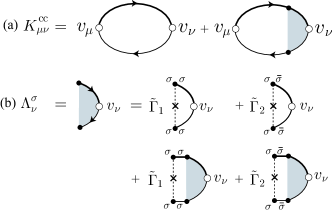
Figure 1: (a) Diagrammatic expression of $K^{\rm cc}_{\mu\nu}$. The thick (thin) solid line represents an electron line carrying Matsubara frequency $i\varepsilon_{n}+i\omega_{\lambda}$ $(i\varepsilon_{n})$. The shaded part represents the vertex function, $\Lambda^{\sigma}_{\nu}$. (b) Dyson equation for $\Lambda^{\sigma}_{\nu}$. The dotted lines represent impurity scattering, either with ($\tilde{\Gamma}_{2}$) or without ($\tilde{\Gamma}_{1}$) spin-flip scattering.

III.2 Result

III.2.1 Charge channel

The response functions $K^{\rm cc}_{\mu\nu}({\bm{q}},\omega+i0)$ [Eq. (20)] for the electric density/current are obtained as

$$K^{\rm cc}_{00} = q^{2}K,$$ (29)

$$K^{\rm cc}_{i0} = K^{\rm cc}_{0i}=q_{i}\omega K,$$ (30)

$$K^{\rm cc}_{ij} = i\omega\left\{\langle D\nu\rangle\left(\delta_{ij}-\frac{q_{i}q_{j}}{q^{2}}\right)-i\omega K\frac{q_{i}q_{j}}{q^{2}}\right\},$$ (31)

where

$$K=\frac{\langle D\nu\bar{Y}\rangle+2\pi\tilde{\Gamma}_{2}\langle\nu\rangle\langle D\nu\rangle}{Y_{\uparrow}Y_{\downarrow}+2\pi\tilde{\Gamma}_{2}\langle Y\nu\rangle}.$$ (32)

The following properties are seen.

(i) Gauge invariance Schrieffer64 and charge conservation are satisfied,

$$K^{\rm cc}_{\mu\nu}q_{\nu}=0,~{}~{}q_{\mu}K^{\rm cc}_{\mu\nu}=0,$$ (33)

where $q_{\mu}=(-\omega,{\bm{q}})$ is a four wavevector.note2

(ii) For $\tilde{\Gamma}_{2}=0$ (without spin-flip scattering), we have

$$K=\frac{\langle D\nu\bar{Y}\rangle}{Y_{\uparrow}Y_{\downarrow}}=\sum_{\sigma}\frac{D_{\sigma}\nu_{\sigma}}{D_{\sigma}q^{2}-i\omega}.$$ (34)

This means that up- and down-spin electrons diffuse independently, and there are two independent diffusion modes.

(iii) For $\tilde{\Gamma}_{2}\neq 0$, and in the long-wavelength and low-frequency limit, $\tau_{\rm sf}^{-1}\equiv 2\pi\tilde{\Gamma}_{2}\langle\nu\rangle/\hbar\gg|Y_{\sigma}|$, we have

$$K=\frac{\langle\nu\rangle\langle D\nu\rangle}{\langle D\nu\rangle q^{2}-i\omega\langle\nu\rangle}=\frac{\sigma_{\rm c}/e^{2}}{D_{\rm eff}q^{2}-i\omega}$$ (35)

where

$$D_{\rm eff}=\frac{\langle D\nu\rangle}{\langle\nu\rangle}=\frac{D_{\uparrow}\nu_{\uparrow}+D_{\downarrow}\nu_{\downarrow}}{\nu_{\uparrow}+\nu_{\downarrow}}$$ (36)

is the effective diffusion constant, and

$$\sigma_{\rm c}=e^{2}\langle D\nu\rangle=e^{2}\sum_{\sigma}D_{\sigma}\nu_{\sigma}$$ (37)

is the electrical conductivity. There is only one diffusion mode owing to the spin mixing $\tilde{\Gamma}_{2}$. In the opposite limit, $\tau_{\rm sf}^{-1}\ll|Y_{\sigma}|$, we have the behavior (34).

Finally, the charge density $\rho\equiv\langle j_{0}({\bm{q}})\rangle_{\omega}$ and the current density ${\bm{j}}\equiv\langle j_{i}({\bm{q}})\rangle_{\omega}$ are given by

$$\rho = -e^{2}K{\rm div}{\bm{E}},$$ (38)

$${\bm{j}} = \sigma_{\rm c}{\bm{E}}+e^{2}\frac{\langle D^{2}\nu\bar{Y}\rangle+2\pi\tilde{\Gamma}_{2}\langle D\nu\rangle^{2}}{Y_{\uparrow}Y_{\downarrow}+2\pi\tilde{\Gamma}_{2}\langle Y\nu\rangle}\nabla({\rm div}{\bm{E}}),$$ (39)

where ${\bm{E}}({\bm{q}},\omega)$ is a Fourier component of the electric field: ${\bm{E}}({\bm{q}},\omega)=-i{\bm{q}}\phi^{\rm em}({\bm{q}},\omega)+i\omega{\bm{A}}^{\rm em}({\bm{q}},\omega)$ with ${\rm div}{\bm{E}}=i{\bm{q}}\cdot{\bm{E}}$ and $\nabla({\rm div}{\bm{E}})=i{\bm{q}}(i{\bm{q}}\cdot{\bm{E}})$.

III.2.2 Spin channel

The response functions $K^{\rm sc}_{\mu\nu}({\bm{q}},\omega+i0)$ [Eq. (122)] for spin density/currents are obtained as

$$K^{\rm sc}_{00} = q^{2}(K^{\rm s}+\Delta K^{\rm s}),$$ (40)

$$K^{\rm sc}_{0i} = q_{i}\omega(K^{\rm s}+\Delta{K}^{\rm s}),$$ (41)

$$K^{\rm sc}_{i0} = q_{i}\omega K^{\rm s},$$ (42)

$$K^{\rm sc}_{ij} = i\omega\left\{\langle\sigma D\nu\rangle\left(\delta_{ij}-\frac{q_{i}q_{j}}{q^{2}}\right)-i\omega K^{\rm s}\frac{q_{i}q_{j}}{q^{2}}\right\},$$ (43)

with

$$K^{\rm s} = \frac{\langle\sigma D\nu\bar{Y}\rangle+2\pi\tilde{\Gamma}_{2}\langle\nu\rangle\langle\sigma D\nu\rangle}{Y_{\uparrow}Y_{\downarrow}+2\pi\tilde{\Gamma}_{2}\langle Y\nu\rangle},$$ (44)

$$K^{\rm s}+\Delta K^{\rm s} = \frac{\langle\sigma D\nu\bar{Y}\rangle+2\pi\tilde{\Gamma}_{2}\langle\sigma\nu\rangle\langle D\nu\rangle}{Y_{\uparrow}Y_{\downarrow}+2\pi\tilde{\Gamma}_{2}\langle Y\nu\rangle}.$$ (45)

The difference

$$\Delta K^{\rm s} = 2\pi\tilde{\Gamma}_{2}\frac{\langle\sigma\nu\rangle\langle D\nu\rangle-\langle\nu\rangle\langle\sigma D\nu\rangle}{Y_{\uparrow}Y_{\downarrow}+2\pi\tilde{\Gamma}_{2}\langle Y\nu\rangle}$$ (46)

$$= 2\pi\tilde{\Gamma}_{2}(\sigma_{\rm c}\nu_{-}-\sigma_{\rm s}\nu_{+})/Ze^{2}$$

$$= 2\pi\tilde{\Gamma}_{2}\nu_{+}\sigma_{\rm c}(P_{\nu}-P_{j})/Ze^{2}$$

arises if $\tilde{\Gamma}_{2}\neq 0$ (and $P_{\nu}\neq P_{j}$). In Eq. (46),

$$\sigma_{\rm s}=e^{2}\langle\sigma D\nu\rangle=e^{2}\sum_{\sigma}\sigma D_{\sigma}\nu_{\sigma}$$ (47)

is the ‘spin conductivity’, and $P_{\nu}=\nu_{-}/\nu_{+}$ and $P_{j}=\sigma_{\rm s}/\sigma_{\rm c}$ represent spin asymmetry in the density of states and in current density, respectively, which are different in general. The following properties are seen.

(i) Gauge invariance is satisfied,

$$K^{\rm sc}_{\mu\nu}q_{\nu}=0,$$ (48)

but spin conservation is not,

$$q_{\mu}K^{\rm sc}_{\mu\nu}=-\left(q^{2}\delta_{\nu 0}+\omega q_{i}\delta_{\nu i}\right)\omega\Delta{K}^{\rm s}\neq 0,$$ (49)

if $\tilde{\Gamma}_{2}\neq 0$, where $i$ is a space component.subscripts2

(ii) Depending on the relative magnitude of $\tau_{\rm sf}^{-1}$ and $|Y_{\sigma}|$, there are two regimes similarly to the charge channel. More interestingly, however, for $\tau_{\rm sf}^{-1}\gg|Y_{\sigma}|$, the magnitudes of $\rho_{\rm s}$ and ${\bm{j}}_{\rm s}$ can be independent, governed, respectively, by asymmetry in density of states and by asymmetry in conductivity; $\rho_{\rm s}\propto P_{\nu}\sigma_{\rm c}$ and ${\bm{j}}_{\rm s}\propto\sigma_{\rm s}$.

Finally, the spin density $\rho_{\rm s}\equiv\langle j_{{\rm s},0}({\bm{q}})\rangle_{\omega}$ and the spin-current density ${\bm{j}}_{\rm s}\equiv\langle j_{{\rm s},i}({\bm{q}})\rangle_{\omega}$ are given by

$$\rho_{\rm s} = -e^{2}({K}^{\rm s}+\Delta{K}^{\rm s}){\rm div}{\bm{E}},$$ (50)

$${\bm{j}}_{\rm s} = \sigma_{\rm s}{\bm{E}}+e^{2}\frac{\langle\sigma D^{2}\nu\bar{Y}\rangle+2\pi\tilde{\Gamma}_{2}\langle D\nu\rangle\langle\sigma D\nu\rangle}{Y_{\uparrow}Y_{\downarrow}+2\pi\tilde{\Gamma}_{2}\langle Y\nu\rangle}\nabla({\rm div}{\bm{E}}).$$

III.2.3 Spin-resolved channel

From Eqs. (38), (39), (50) and (III.2.2), we obtain the “spin-resolved” density and current,

$$\rho_{\sigma}=-e^{2}K_{\sigma}{\rm div}{\bm{E}},$$ (52)

$${\bm{j}}_{\sigma}=\sigma_{\sigma}{\bm{E}}+e^{2}D_{\sigma}K_{\sigma}\nabla({\rm div}{\bm{E}}),$$ (53)

where

$$K_{\sigma}=\frac{D_{\sigma}Y_{\bar{\sigma}}+2\pi\tilde{\Gamma}_{2}\langle{D\nu}\rangle}{Y_{\uparrow}Y_{\downarrow}+2\pi\tilde{\Gamma}_{2}\langle Y\nu\rangle}\nu_{\sigma}.$$ (54)

From Eqs. (52) and (53), we may derive

$${\bm{j}}_{\sigma}=\sigma_{\sigma}{\bm{E}}-D_{\sigma}\nabla\rho_{\sigma}$$ (55)

where

$$\sigma_{\sigma}=e^{2}D_{\sigma}\nu_{\sigma}$$ (56)

is the “spin-resolved” conductivity. Further discussion will be given in Sec. VI.

IV Spin and Charge Transport in time-dependent spin texture

In the previous section, we studied spin and charge transport in a ferromagnetic conductor in its uniformly magnetized state. In the second part of this paper, which consists of Sec. IV and Sec. V, we consider a more general case in which the magnetization varies in space and time. This magnetic texture and dynamics induce density change and current even if $A_{\mu}^{\rm em}$ is absent, which are calculated in this paper in the first order in both spatial gradient and time derivative.

IV.1 Transformation to local spin frame

To treat the effects of space- and time-dependent magnetization, we introduce a local spin frame where the spin quantization axis of $s$-electrons is taken to be the $d$-spin direction ${\bm{n}}(x)$ at each space-time point. KMP77 ; Volovik87 ; TF94 The original spinor $c$ is then transformed to a spinor $a$ in the new frame (rotated frame) as $c=Ua$, where $U$ is a 2 $\times$ 2 unitary matrix satisfying $c^{\dagger}({\bm{n}}\cdot{\bm{\sigma}})\,c=a^{\dagger}\sigma^{z}a$. It is convenient to take $U={\bm{m}}\cdot{\bm{\sigma}}$ with

$${\bm{m}}=\left(\sin\frac{\theta}{2}\cos\phi,~{}\sin\frac{\theta}{2}\sin\phi,~{}\cos\frac{\theta}{2}\right),$$ (57)

where $\theta$ and $\phi$ are ordinary spherical angles parametrizing ${\bm{n}}$. From space/time derivatives, $\partial_{\mu}c=U(\partial_{\mu}+iA_{\mu})a$, there arises an SU(2) gauge field

$$A_{\mu}=-iU^{\dagger}\partial_{\mu}U=A_{\mu}^{\alpha}\sigma^{\alpha}.$$ (58)

This is an effective gauge field, which represents space/time variations of magnetization. The Lagrangian in the rotated frame is then given by $L=\tilde{L}_{\rm el}-H_{\rm e-A}$,

$$\tilde{L}_{\rm el}=\int d{\bm{r}}~{}a^{\dagger}\left[i\hbar\frac{\partial}{\partial t}+\frac{\hbar^{2}}{2m}\nabla^{2}+\varepsilon_{\rm F}-\tilde{V}_{\rm imp}+M\sigma^{z}\right]a,$$

(59)

$$H_{\rm e-A}=-\frac{\hbar}{e}\int d{\bm{r}}~{}\tilde{j}^{\alpha}_{\mu}A^{\alpha}_{\mu}+\frac{\hbar^{2}}{2m}\int d{\bm{r}}~{}A^{\alpha}_{i}A^{\alpha}_{i}a^{\dagger}a,$$ (60)

where $\tilde{j}^{\alpha}_{\mu}=(\tilde{\rho}^{\alpha},\,\tilde{\bm{j}}^{\alpha})$ is a four current representing spin and spin-current densities (“paramagnetic” component) in the rotated frame,

$$\tilde{\rho}^{\alpha}=-ea^{\dagger}\sigma^{\alpha}a\ \ (\ =\,\tilde{j}^{\alpha}_{0}),$$ (61)

$$\tilde{\bm{j}}^{\alpha}=-e\frac{\hbar}{2mi}\,a^{\dagger}\sigma^{\alpha}\overset{\leftrightarrow}{\nabla}a.$$ (62)

The spin part of the impurity potential $\tilde{V}_{\rm imp}$ is expressed as $S^{\alpha}_{j}(c^{\dagger}\sigma^{\alpha}c)=\tilde{S}^{\alpha}_{j}(t)(a^{\dagger}\sigma^{\alpha}a)$, where $\tilde{S}_{j}^{\alpha}(t)={\cal R}^{\alpha\beta}({\bm{R}}_{j}^{\prime},t)S^{\beta}_{j}$ is the impurity spin in the rotated frame KS07 with

$${\cal R}^{\alpha\beta}=2m^{\alpha}m^{\beta}-\delta^{\alpha\beta}$$ (63)

being a $3\times 3$ orthogonal matrix representing the same rotation as $U$. Hereafter, the anisotropy axis of impurity spins is defined in reference to the rotated frame

$$\overline{\tilde{S}_{i}^{\alpha}\tilde{S}_{j}^{\beta}}=\delta_{ij}\delta^{\alpha\beta}\times\left\{\begin{array}[]{cc}\overline{S_{\perp}^{2}}&(\alpha,\beta=x,y)\\ \overline{S_{z}^{2}}&(\alpha,\beta=z)\end{array}\right..$$ (64)

IV.2 Effective U(1) gauge field

There is some arbitrariness in the choice of the rotated frame; one could take $c=U^{\prime}a^{\prime}$ with $U^{\prime}=Ue^{-i\sigma^{z}\chi/2}$, where $\chi$ is an arbitrary function of $x$. This arbitrariness is a gauge degree of freedom in the sense that physical quantities should not depend on it. It is in fact expressed as the gauge transformation on $a$ and $A_{\mu}$,

$$a^{\prime} = e^{-i\sigma^{z}\chi/2}a,$$ (65)

$$A^{\prime}_{\mu} = -i(U^{\prime})^{\dagger}\partial_{\mu}U^{\prime}$$ (66)

$$= e^{i\sigma^{z}\chi/2}A_{\mu}e^{-i\sigma^{z}\chi/2}-\sigma^{z}\partial_{\mu}\chi/2,$$

or, in componentwise,

$$A^{\prime x}_{\mu}+iA^{\prime y}_{\mu} = e^{-i\chi}\left(A^{x}_{\mu}+iA^{y}_{\mu}\right),$$ (67)

$$A^{\prime z}_{\mu} = A^{z}_{\mu}-\partial_{\mu}\chi/2.$$ (68)

Note that its $z$ component $A^{z}_{\mu}$ transforms like a gauge potential in ordinary electromagnetism, hence can be regarded as a U(1) gauge field. In the following, when we refer to gauge transformation, it means Eqs. (65)-(68). In the next subsection, we study spin and charge transport driven by magnetization dynamics as a linear response to this effective gauge field $A^{z}_{\mu}$.

Generally, one can do a gradient expansion in terms of $A^{\alpha}_{\mu}$. The expansion parameter is $qv_{{\rm F}\sigma}\tau_{\sigma}$ and $\omega\tau_{\sigma}$ (for $A^{z}_{\mu}$),SK09 where $q^{-1}$ and $\omega$ are characteristic length and frequency, respectively, of the magnetic texture. In this work, we consider only the lowest nontrivial order in the expansion by assuming $qv_{{\rm F}\sigma}\tau_{\sigma}\ll 1$ and $\omega\tau_{\sigma}\ll 1$. This condition coincides with the condition, $|X_{\sigma}|=|D_{\sigma}q^{2}-i\omega|\tau_{\sigma}\ll 1$, declared below Eq. (12). In typical experiments with Permalloy ($v_{{\rm F}\sigma}\sim 10^{5}$m/s, $\tau_{\sigma}\sim 10^{-14}$s) Bass-Pratt07 , $q^{-1}\sim$ 100 nm, $\omega\sim$ 100 MHz YBKXNTE09 , we have $D_{\sigma}q^{2}\tau\sim 10^{-4}$ and $\omega\tau_{\sigma}\sim 10^{-6}$, and the above conditions are satisfied quite well.

IV.3 Linear response to $A^{\rm em}_{\mu}$ and $A^{z}_{\mu}$.

Let us examine the density/current response to the two gauge fields, $A^{\rm em}_{\mu}$ and $A^{z}_{\mu}$. Spin density and currents considered here are the ones whose spin is projected on ${\bm{n}}$ (or $\hat{z}$ in the rotated frame), i.e., $\rho_{\rm s}=\tilde{\rho}^{\,z}$ and $\tilde{{\bm{j}}}_{\rm s}=\tilde{{\bm{j}}}^{z}$. The total current densities contain the gauge fields,

$$j_{\mu} = (\,\rho\,,\,\tilde{\bm{j}}+(e\rho{\bm{A}}^{\rm em}+\hbar\tilde{\rho}^{\alpha}{\bm{A}}^{\alpha})/m),$$ (69)

$$j_{{\rm s},\mu} = (\,\rho_{\rm s}\,,\,\tilde{\bm{j}}_{\rm s}+(e\rho_{\rm s}{\bm{A}}^{\rm em}+\hbar\rho{\bm{A}}^{z})/m),\ \$$ (70)

for charge and spin channels, where $\rho=-ea^{\dagger}a$ and $\tilde{\bm{j}}=(-e\hbar/2mi)\,a^{\dagger}\overset{\leftrightarrow}{\nabla}a$. By generalizing Eqs. (18) and (19), we may write

$$\langle j_{\mu}({\bm{q}})\rangle_{\omega} = e^{2}\tilde{K}^{\rm cc}_{\mu\nu}A^{\rm em}_{\nu}+e\hbar\tilde{K}^{\rm cs}_{\mu\nu}A^{z}_{\nu},$$ (71)

$$\langle j_{{\rm s},\mu}({\bm{q}})\rangle_{\omega} = e^{2}\tilde{K}^{\rm sc}_{\mu\nu}A^{\rm em}_{\nu}+e\hbar\tilde{K}^{\rm ss}_{\mu\nu}A^{z}_{\nu}.$$ (72)

The response functions, $\tilde{K}^{\rm cc}_{\mu\nu}$ and $\tilde{K}^{\rm sc}_{\mu\nu}$, are obtained from Eqs. (20) and (21) by replacing the electron operators in the original frame, $c$ $(c^{\dagger})$, by those in the rotated frame, $a$ $(a^{\dagger})$, and are already calculated as $K^{\rm cc}_{\mu\nu}$ and $K^{\rm sc}_{\mu\nu}$ in Sec. III. Thus the response to $A^{\rm em}_{\mu}$ in Eqs. (71) and (72) exactly follows the results there.

Let us then focus on the response to $A^{z}_{\mu}$, in particular, on $\tilde{K}^{\rm cs}_{\mu\nu}$. ($\tilde{K}^{\rm ss}_{\mu\nu}$ will be presented in Appendix D.) From the definition (linear-response formula), one can show that the Onsager’s reciprocity relations hold,

$$\tilde{K}^{\rm cs}_{\mu\nu}({\bm{q}},i\omega_{\lambda})=\tilde{K}^{\rm sc}_{\nu\mu}(-{\bm{q}},-i\omega_{\lambda}),$$ (73)

or

$$\tilde{K}^{\rm cs}_{\mu\nu}({\bm{q}},\omega+i0)=\tilde{K}^{\rm sc}_{\nu\mu}(-{\bm{q}},-\omega-i0).$$ (74)

From this, we see that

$$q_{\mu}\tilde{K}^{\rm cs}_{\mu\nu}=\tilde{K}^{\rm sc}_{\nu\mu}q_{\mu}=0,$$ (75)

namely, the charge conservation is satisfied also in the response to $A^{z}_{\mu}$. On the other hand, if $\tilde{\Gamma}_{2}\neq 0$, spin is not conserved, $q_{\nu}\tilde{K}^{\rm sc}_{\nu\mu}\neq 0$ as seen before. This fact, combined with Eq. (74), implies that $\tilde{K}^{\rm cs}_{\mu\nu}$ is not gauge invariant,

$$\tilde{K}^{\rm cs}_{\mu\nu}q_{\nu}=q_{\nu}\tilde{K}^{\rm sc}_{\nu\mu}\neq 0,$$ (76)

if $\tilde{\Gamma}_{2}\neq 0$. The gauge non-invariant terms in Eq. (71) may be extracted assubscripts2

$$j_{\mu}^{\prime}({\bm{q}},\omega)=e\hbar\Delta K^{\rm s}\{q^{2}\delta_{\mu 0}+q_{i}\omega\delta_{\mu i}\}A^{z}_{{\bm{q}},0}.$$ (77)

To summarize, the calculation based on the gauge field $A^{z}_{\mu}$ fails to respect gauge invariance in the presence of spin-flip scattering. Stated more explicitly, the density and current calculated as a linear response to $A^{z}_{\mu}$ are not gauge invariant.note3

V Careful treatment of spin relaxation effects

V.1 Restoration of gauge invariance

The lack of gauge invariance encountered in Sec. IV-C is due to an oversight of some contributions. We recall that the quenched magnetic impurities in the original frame become time-dependent in the rotated frame, $\tilde{S}_{j}(t)={\cal R}^{\alpha\beta}({\bm{R}}^{\prime}_{j},t)S^{\beta}_{j}$. Therefore, we should treat the spin part of the impurity potential

$$H_{\rm s}=u_{\rm s}\sum_{j}\int d{\bm{r}}\tilde{{\bm{S}}}_{j}(t)\delta({\bm{r}}-{\bm{R}}^{\prime}_{j})\cdot(a^{\dagger}{\bm{\sigma}}a)_{x}$$ (78)

as a time-dependent perturbation. The same situation was met in the calculation of Gilbert damping. KS07

Since the first-order (linear) response vanishes, $\overline{\tilde{S}^{\alpha}_{j}(t)}=0$, let us consider the second-order (nonlinear) response,

$$\Delta j_{\mu}({\bm{q}},\omega)$$

$$= -en_{\rm s}u_{\rm s}^{2}\int_{-\infty}^{\infty}\frac{d\omega^{\prime}}{2\pi}\chi^{\alpha\beta}_{\mu}({\bm{q}};\omega,\omega^{\prime})\overline{\big{[}\tilde{S}^{\alpha}(\omega-\omega^{\prime})\tilde{S}^{\beta}(\omega^{\prime})\big{]}}_{{\bm{q}}}$$

where $\tilde{S}^{\alpha}_{{\bm{p}}}(\omega)$ is the Fourier component of $\sum_{j}\tilde{S}^{\alpha}_{j}(t)\,\delta({\bm{r}}-{\bm{R}}_{j}^{\prime})$, and $\chi_{\mu}^{\alpha\beta}$ is the nonlinear response function. KS07 To calculate it, it is simpler to use the path-ordered Green’s function.Rammer86 The contribution represented in Fig. 2 are given by

$$\chi_{\mu}^{\alpha\beta}({\bm{q}};\omega,\omega^{\prime})=\sum_{{\bm{k}},{\bm{k}}^{\prime}}\int_{-\infty}^{\infty}\frac{d\varepsilon}{2\pi i}$$

$$\times{\rm tr}[(v_{\mu}+\Lambda_{\mu})G_{{\bm{k}}_{+}}(\varepsilon_{+})\sigma^{\alpha}G_{{\bm{k}}^{\prime}}(\varepsilon+\omega^{\prime})\sigma^{\beta}G_{{\bm{k}}_{-}}(\varepsilon)]^{<}$$

(80)

where $\varepsilon_{+}=\varepsilon+\omega$. The Green’s function $G_{{\bm{k}}}(\varepsilon)$ now stands for a path-ordered one, whose lesser component is given by

$$G^{<}_{{\bm{k}}}(\varepsilon)=f(\varepsilon)(G^{\rm A}_{{\bm{k}}}(\varepsilon)-G^{\rm R}_{{\bm{k}}}(\varepsilon)),$$ (81)

with $f(\varepsilon)$ being the Fermi distribution function. In Eq. (80), we adopt a matrix notaion, $(G)_{\sigma,\sigma^{\prime}}=G_{\sigma}\delta_{\sigma\sigma^{\prime}}$, $(\Lambda_{\mu})_{\sigma,\sigma^{\prime}}=\Lambda_{\mu}^{\sigma}\delta_{\sigma\sigma^{\prime}}$ with $\Lambda_{\mu}^{\sigma}$ given by Eq. (120), and ‘tr’ means trace in spin space.

We expand $\chi^{\alpha\beta}_{\mu}({\bm{q}};\omega,\omega^{\prime})$ with respect to $\omega$ and $\omega^{\prime}$ as

$$\chi^{\alpha\beta}_{\mu}({\bm{q}};\omega,\omega^{\prime})=A^{\alpha\beta}_{\mu}-i\omega B^{\alpha\beta}_{\mu}-i\omega^{\prime}C^{\alpha\beta}_{\mu}+\cdots$$ (82)

where $A^{\alpha\beta}_{\mu}$, $B^{\alpha\beta}_{\mu}$ and $C^{\alpha\beta}_{\mu}$ are the expansion coefficients. Substituting Eq. (82) into Eq. (V.1), we have

$$\Delta j_{\mu}({\bm{q}},\omega) = -en_{\rm s}u_{\rm s}^{2}\left[B^{\alpha\beta}_{\mu}\overline{\partial_{t}(\tilde{S}^{\alpha}\tilde{S}^{\beta})}+C^{\alpha\beta}_{\mu}\,\overline{\tilde{S}^{\alpha}\partial_{t}\tilde{S}^{\beta}}\,\right]_{{\bm{q}},\omega}$$

where $\tilde{\bm{S}}=\tilde{\bm{S}}(t)$ is time dependent. (We have dropped a term containing $A^{\alpha\beta}_{\mu}$, which does not reflect the time dependence of $\tilde{\bm{S}}(t)$.) From

$$\overline{\tilde{S}^{\alpha}\partial_{t}\tilde{S}^{\beta}}=(\overline{S^{2}_{\perp}}\delta^{\alpha\gamma}_{\perp}+\overline{S^{2}_{z}}\,\delta^{\alpha z}\delta^{\gamma z})({\cal R}\partial_{t}{\cal R})^{\gamma\beta},$$ (84)

where $\delta^{\alpha\beta}_{\perp}=\delta^{\alpha\beta}-\delta^{\alpha z}\delta^{\beta z}$, and the relationKS07

$$({\cal R}\partial_{\mu}{\cal R})^{\alpha\beta}=2\varepsilon^{\alpha\beta\gamma}A^{\gamma}_{\mu},$$ (85)

we see that Eq. (LABEL:extra-current-1) describes a response to $A^{\gamma}_{0}$. The coefficients are calculated as subscripts2 (see Appendix B)

$$B^{\alpha\beta}_{\mu} = -\frac{1}{2}\,C^{\alpha\beta}_{\mu},$$ (86)

$$= \pi\nu_{\uparrow}\nu_{\downarrow}\frac{\langle\sigma Y\rangle\,\delta_{\mu 0}+iq_{i}\langle\sigma D\bar{Y}\rangle\,\delta_{\mu i}}{Y_{\uparrow}Y_{\downarrow}+2\pi\tilde{\Gamma}_{2}\langle Y\nu\rangle}\,\varepsilon^{\alpha\beta}\,$$

where $\varepsilon^{\alpha\beta}=\varepsilon^{\alpha\beta z}$, and we have dropped unimportant terms proportional to $\delta^{\alpha\beta}_{\perp}$ or $\delta^{\alpha z}\delta^{\gamma z}$.

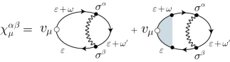
Figure 2: Diagrammatic expression of $\chi^{\alpha\beta}_{\mu}$. The wavy line represents scattering from impurity spins, which are time-dependent in the rotated frame. The shaded part represents the vertex function $\Lambda^{\sigma}_{\mu}$.

We thus have

$$\Delta j_{\mu}({\bm{q}},\omega) = e\hbar\Delta\tilde{K}^{\rm cs}_{\mu\nu}A^{z}_{{\bm{q}},\nu},$$ (87)

withsubscripts2

$$\Delta\tilde{K}^{\rm cs}_{\mu\nu} = -\Delta K^{\rm s}\{q^{2}\delta_{\mu 0}+q_{i}\omega\delta_{\mu i}\}\delta_{\nu 0}.$$ (88)

This new contribution cancels the gauge-dependent terms, Eq. (77), and restores the gauge invariance,

$$(\tilde{K}^{\rm cs}_{\mu\nu}+\Delta\tilde{K}^{\rm cs}_{\mu\nu})q_{\nu}=0.$$ (89)

Note that it does not affect the charge conservation since $q_{\mu}\Delta\tilde{K}^{\rm cs}_{\mu\nu}=0$, nor the spin non-conservation ($q_{\mu}\tilde{K}^{\rm sc}_{\mu\nu}\neq 0$) since it does not contribute to $\tilde{K}^{\rm sc}_{\mu\nu}$.

The gauge-invariant result for the charge density $\rho^{{\rm smf}\,(1)}({\bm{q}},\omega)$ and current density ${\bm{j}}^{{\rm smf}\,(1)}({\bm{q}},\omega)$ induced by magnetization dynamics is summarized as

$$\rho^{\rm smf\,(1)} = -e^{2}K^{\rm s}{\rm div}{\bm{E}}_{\rm s}^{0},$$ (90)

$${\bm{j}}^{\rm smf\,(1)} = \sigma_{\rm s}{\bm{E}}_{\rm s}^{0}$$

$$+ e^{2}\frac{\langle\sigma D^{2}\nu\bar{Y}\rangle+2\pi\tilde{\Gamma}_{2}\langle D\nu\rangle\langle\sigma D\nu\rangle}{Y_{\uparrow}Y_{\downarrow}+2\pi\tilde{\Gamma}_{2}\langle Y\nu\rangle}\nabla({\rm div}{\bm{E}}_{\rm s}^{0}).$$

The first term on the right-hand side of Eq. (V.1) has the form of Eq. (3), and implies the existence of spin-dependent motive force described by the effective ‘electric’ field ${\bm{E}}_{\rm s}^{0}$. The second term of Eq. (V.1) represents a diffusion current arising from charge imbalance induced by ${\bm{E}}_{\rm s}^{0}$, as made clear in Sec. VI. This term implies the existence of nonlocal spin-transfer torque as the reciprocal effect, whose study will be left to the future.

V.2 Dissipative correction

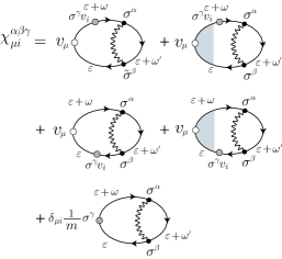
Figure 3: Diagrammatic expression of $\chi^{\alpha\beta\gamma}_{\mu i}$. The gray circle represents the interaction with $A_{\mu}^{\gamma}$.

It is important to note that there is one more contribution within the same order in gradient expansion. It is essentially given by Eq. (V.1), but with one more factor of $A_{\mu}^{\alpha}$. The response function, denoted by $\chi^{\alpha\beta\gamma}_{\mu i}$, is obtained from Eq. (80) by further extracting $A_{\mu}^{\alpha}$ via Eq. (60). These are expressed as [Fig. 3]

$$j^{{\rm smf}\,(2)}_{\mu}({\bm{q}},\omega) = -e\hbar n_{\rm s}u_{\rm s}^{2}\sum_{{\bm{q}}^{\prime}}\int_{-\infty}^{\infty}\frac{d\omega^{\prime}}{2\pi}\chi^{\alpha\beta\gamma}_{\mu i}({\bm{q}};\omega,\omega^{\prime})$$ (92)

$$\times \overline{\big{[}\tilde{S}^{\alpha}(\omega-\omega^{\prime})\tilde{S}^{\beta}(\omega^{\prime})\big{]}}_{{\bm{q}}-{\bm{q}}^{\prime}}A^{\gamma}_{{\bm{q}}^{\prime},i},$$

where

$$\chi^{\alpha\beta\gamma}_{\mu i}({\bm{q}};\omega,\omega^{\prime})=\sum_{{\bm{k}},{\bm{k}}^{\prime}}\int_{-\infty}^{\infty}\frac{d\varepsilon}{2\pi i}\,{\rm tr}\Big{[}(v_{\mu}+\Lambda_{\mu})$$ (93)

$$\times \{v_{i}^{+}G_{{\bm{k}}+}(\varepsilon_{+})\sigma^{\gamma}G_{{\bm{k}}+}(\varepsilon_{+})\sigma^{\alpha}G_{{\bm{k}}^{\prime}}(\varepsilon+\omega^{\prime})\sigma^{\beta}G_{{\bm{k}}-}(\varepsilon)$$

$$+v_{i}^{-}G_{{\bm{k}}+}(\varepsilon_{+})\sigma^{\alpha}G_{{\bm{k}}^{\prime}}(\varepsilon+\omega^{\prime})\sigma^{\beta}G_{{\bm{k}}-}(\varepsilon)\sigma^{\gamma}G_{{\bm{k}}-}(\varepsilon)\}$$

$$+ \frac{1}{m}\,\delta_{\mu i}\sigma^{\gamma}G_{{\bm{k}}+}(\varepsilon_{+})\sigma^{\alpha}G_{{\bm{k}}^{\prime}}(\varepsilon+\omega^{\prime})\sigma^{\beta}G_{{\bm{k}}-}(\varepsilon)\Big{]}^{<},$$

with $v_{i}^{\pm}=(k_{i}\pm q_{i}/2)/m$. We have put ${\bm{q}}^{\prime}={\bm{0}}$ in Eq. (93), but retained ${\bm{q}}$ and $\omega$. Note that the terms with $\gamma=z$ cancel out, and $A_{\mu}^{z}$ does not contribute. In the same way as Sec. V-A, we expand $\chi^{\alpha\beta\gamma}_{\mu i}$ with respect to $\omega$ and $\omega^{\prime}$ as $\chi^{\alpha\beta\gamma}_{\mu i}=A^{\alpha\beta\gamma}_{\mu i}-i\omega B^{\alpha\beta\gamma}_{\mu i}-i\omega^{\prime}C^{\alpha\beta\gamma}_{\mu i}+\cdots$ and focus on the coefficients $B^{\alpha\beta\gamma}_{\mu i}$ and $C^{\alpha\beta\gamma}_{\mu i}$. Deferring the details to Appendix C, we cite the result

$$B^{\alpha\beta\gamma}_{\mu i} = -\frac{1}{2}\,C^{\alpha\beta\gamma}_{\mu i}$$ (94)

$$= (\delta^{\alpha z}\varepsilon^{\beta\gamma}-\delta^{\beta z}\varepsilon^{\alpha\gamma})\frac{\nu_{+}}{4M}\sum_{\sigma}\sigma(L^{\sigma}_{i\mu})^{\rm RA},\ \$$

where $\nu_{+}=\nu_{\uparrow}+\nu_{\downarrow}$, and $L^{\sigma}_{i\mu}$’s are given by Eqs. (129) and (131). Note the order of the subscripts, $i\mu$. We thus have

$$j_{\mu}^{{\rm smf}\,(2)}({\bm{q}},\omega)=\beta\frac{e\hbar}{\pi}\sum_{\sigma}\sigma(L^{\sigma}_{i\mu})^{\rm RA}({\bm{A}}^{\perp}_{i}\!\cdot\!{\bm{A}}^{\perp}_{0})_{{\bm{q}},\omega}$$ (95)

where ${\bm{A}}^{\perp}_{\mu}={\bm{A}}_{\mu}-\hat{z}\,(\hat{z}\!\cdot\!{\bm{A}}_{\mu})$, and

$$\beta=\frac{\pi}{M}n_{\rm s}u_{\rm s}^{2}(\overline{S_{\perp}^{2}}+\overline{S_{z}^{2}})(\nu_{\uparrow}+\nu_{\downarrow})$$ (96)

is a measure of spin relaxation. With the relation

$${\bm{A}}^{\perp}_{i}\!\cdot{\bm{A}}^{\perp}_{0}=\frac{1}{4}\,\dot{{\bm{n}}}\!\cdot\partial_{i}{\bm{n}},$$ (97)

which is gauge-invariant under (67), we finally obtain

$$\rho^{\rm smf\,(2)} = -e^{2}K_{\rm s}{\rm div}{\bm{E}}^{\rm dis}_{\rm s},$$ (98)

$${\bm{j}}^{{\rm smf}\,(2)} = \sigma_{\rm s}{\bm{E}}^{\rm dis}_{\rm s}$$

$$+ e^{2}\frac{\langle\sigma D^{2}\nu\bar{Y}\rangle+2\pi\tilde{\Gamma}_{2}\langle D\nu\rangle\langle\sigma D\nu\rangle}{Y_{\uparrow}Y_{\downarrow}+2\pi\tilde{\Gamma}_{2}\langle Y\nu\rangle}\nabla({\rm div}{\bm{E}}_{\rm s}^{\rm dis}),$$

(99)

where ${\bm{E}}_{\rm s}^{\rm dis}$ is given by Eq. (2). Since ${\bm{E}}_{\rm s}^{\rm dis}$ contains $\beta$ as a prefactor, Eqs. (98) and (99) come from spin-relaxation processes. This $\beta$ is exactly the same as the coefficient of the $\beta$-term of current-induced torque,KTS06 ; KS07 consistent with the fact that these are reciprocal to each other.Duine08 ; Tserkovnyak08

VI Results and discussion

The results obtained in this paper are summarized as

$$\rho = -\frac{\langle D\nu\bar{Y}F\rangle+2\pi\tilde{\Gamma}_{2}\langle\nu\rangle\langle D\nu F\rangle}{Y_{\uparrow}Y_{\downarrow}+2\pi\tilde{\Gamma}_{2}\langle Y\nu\rangle},$$ (100)

$${\bm{j}} = \sigma_{\rm c}{\bm{E}}+\sigma_{\rm s}{\bm{E}}_{\rm s}$$ (101)

$$+ \frac{\langle D^{2}\nu\bar{Y}\nabla F\rangle+2\pi\tilde{\Gamma}_{2}\langle D\nu\rangle\langle D\nu\nabla F\rangle}{Y_{\uparrow}Y_{\downarrow}+2\pi\tilde{\Gamma}_{2}\langle Y\nu\rangle},$$

$$\rho_{\rm s} = -\frac{\langle\sigma D\nu\bar{Y}F\rangle+2\pi\tilde{\Gamma}_{2}\langle\sigma\nu\rangle\langle D\nu F\rangle}{Y_{\uparrow}Y_{\downarrow}+2\pi\tilde{\Gamma}_{2}\langle Y\nu\rangle},$$ (102)

$${\bm{j}}_{\rm s} = \sigma_{\rm s}{\bm{E}}+\sigma_{\rm c}{\bm{E}}_{\rm s}$$ (103)

$$+ \frac{\langle\sigma D^{2}\nu\bar{Y}\nabla F\rangle+2\pi\tilde{\Gamma}_{2}\langle\sigma D\nu\rangle\langle D\nu\nabla F\rangle}{Y_{\uparrow}Y_{\downarrow}+2\pi\tilde{\Gamma}_{2}\langle Y\nu\rangle},$$

where $F_{\rm c}=e^{2}{\rm div}{\bm{E}}$, $F_{\rm s}=e^{2}{\rm div}{\bm{E}}_{\rm s}$, and $F_{\sigma}=F_{\rm c}+\sigma F_{\rm s}$. The notations are as before; for example, $\langle D\nu\nabla F\rangle=D_{\uparrow}\nu_{\uparrow}\nabla F_{\uparrow}+D_{\downarrow}\nu_{\downarrow}\nabla F_{\downarrow}$. From these relations [or Eqs. (106) and (107) below], we identify the spin motive field to be

$$E_{{\rm s},i}=\frac{\hbar}{2e}\left\{-{\bm{n}}\!\cdot\!(\dot{\bm{n}}\times\partial_{i}{\bm{n}})+\beta(\dot{\bm{n}}\!\cdot\!\partial_{i}{\bm{n}})\right\}.$$ (104)

The spin-resolved density and current are given by

$$\rho_{\sigma} = -e^{2}{\rm div}(K_{\sigma}{\bm{E}}+K_{\sigma}^{\prime}{\bm{E}}_{\rm s}),$$ (105)

$${\bm{j}}_{\sigma} = \sigma_{\sigma}{\bm{E}}_{\sigma}-D_{\sigma}\nabla\rho_{\sigma},$$ (106)

$${\bm{E}}_{\sigma} = {\bm{E}}+\sigma{\bm{E}}_{\rm s},$$ (107)

where ${\bm{E}}_{\sigma}$ is the total field felt by spin-$\sigma$ electrons. The coefficient $K_{\sigma}$ is given by Eq. (54), and $K_{\sigma}^{\prime}$ by

$$K_{\sigma}^{\prime} = \frac{\sigma D_{\sigma}Y_{\bar{\sigma}}+2\pi\tilde{\Gamma}_{2}\langle\sigma D\nu\rangle}{Y_{\uparrow}Y_{\downarrow}+2\pi\tilde{\Gamma}_{2}\langle Y\nu\rangle}\,\nu_{\sigma}.$$ (108)

There are two characteristic regimes depending on the relative magnitude of $\tau_{\rm sf}^{-1}\equiv 2\pi\tilde{\Gamma}_{2}\langle\nu\rangle/\hbar$ and $|Y_{\sigma}|$. For $\tau_{\rm sf}^{-1}\ll|Y_{\sigma}|$, Eq. (105) becomes

$$\rho_{\sigma} \simeq -\frac{\sigma_{\sigma}}{D_{\sigma}q^{2}-i\omega}\,{\rm div}{\bm{E}}_{\sigma},$$ (109)

meaning that the spin-$\sigma$ electrons respond only to ${\bm{E}}_{\sigma}$, not to ${\bm{E}}_{\bar{\sigma}}$, and the two spin components ($\uparrow$ and $\downarrow$) behave independently. In particular, the response to a spin motive field ${\bm{E}}_{\rm s}$ (set ${\bm{E}}={\bm{0}}$ for simplicity) is opposite in sign between $\uparrow$ and $\downarrow$ electrons. In the opposite limit, $\tau_{\rm sf}^{-1}\gg|Y_{\sigma}|$, Eq. (105) becomes

$$\rho_{\sigma} \simeq -\frac{\nu_{\sigma}/\langle\nu\rangle}{D_{\rm eff}q^{2}-i\omega}\,{\rm div}(\sigma_{\uparrow}{\bm{E}}_{\uparrow}+\sigma_{\downarrow}{\bm{E}}_{\downarrow}),$$ (110)

where $D_{\rm eff}=\langle D\nu\rangle/\langle\nu\rangle$. In this case, the density of spin-$\sigma$ electrons is affected not only by ${\bm{E}}_{\sigma}$ but also by ${\bm{E}}_{\bar{\sigma}}$. This is due to the strong spin mixing; as an elementary process, $\rho_{\sigma}$ is induced solely by ${\bm{E}}_{\sigma}$, not ${\bm{E}}_{\bar{\sigma}}$, but subsequent spin-flip processes tends to equilibrate $\rho_{\uparrow}$ and $\rho_{\downarrow}$. Note that $\uparrow$ electrons and $\downarrow$ electrons respond to ${\bm{E}}_{\rm s}$ with the same sign. (The common sign is determined by that of $\sigma_{\uparrow}-\sigma_{\downarrow}$.)

The above features oppose the picture of two independent currents, but they are actually described within the conventional two-current model. Mott64 ; Fert-Campbell68 ; Son87 ; Valet-Fert93 This is best demonstrated by the relation

$$\frac{\partial}{\partial t}\rho_{\sigma}+{\rm div}{\bm{j}}_{\sigma}=-\left(\frac{\rho_{\sigma}}{\tau_{{\rm sf},\sigma}}-\frac{\rho_{\bar{\sigma}}}{\tau_{{\rm sf},\bar{\sigma}}}\right),$$ (111)

where

$$\tau_{{\rm sf},\sigma}^{-1}=2\pi\tilde{\Gamma}_{2}\nu_{\bar{\sigma}}/\hbar$$ (112)

is the spin-flip rate for spin-$\sigma$ electrons. The right-hand side of Eq. (111) represents a coupling between $\uparrow$ and $\downarrow$ electrons. In deriving Eq. (111), we have used Eqs. (105), (106), (108) and (54), and the relations, $\langle\sigma K/\nu\rangle=\langle\sigma D\bar{Y}\rangle/Z$ and $\langle\sigma K^{\prime}/\nu\rangle=\langle D\bar{Y}\rangle/Z$. Note that $\rho_{\sigma}$, being given by Eq. (105), represents a deviation from the equilibrium value. One may define the deviation of chemical potential, $\delta\mu_{\sigma}$, from equilibrium by

$$\rho_{\sigma}=-e\nu_{\sigma}\delta\mu_{\sigma}.$$ (113)

Then Eq. (111) can be put in a familiar form Son87 ; Valet-Fert93

$$\frac{\partial}{\partial t}\rho_{\sigma}+{\rm div}{\bm{j}}_{\sigma} = \frac{\sigma_{\sigma}}{e}\!\cdot\!\frac{\delta\mu_{\sigma}-\delta\mu_{\bar{\sigma}}}{\ell_{\sigma}^{2}}.$$ (114)

where $\ell_{\sigma}=\sqrt{D_{\sigma}\tau_{{\rm sf},\sigma}}$ is the spin diffusion length for spin-$\sigma$ electrons.

The present work is therefore within the two-current picture. This fact was implicitly used in identifying the spin motive force on the basis of Eq. (3).

VII Summary

In this paper, we have studied spin and charge transport in a conducting ferromagnet driven by two kinds of gauge fields, $A^{\rm em}_{\mu}$ and $A^{z}_{\mu}$, which act in charge channel and spin channel, respectively. In particular, we have given a microscopic calculation of spin motive force by taking spin-relaxation effects into account.

In the first part, we calculated density and current in both spin and charge channels in response to the ordinary electromagnetic field $A^{\rm em}_{\mu}$ in a uniformly magnetized state. We observed a crossover from two diffusion modes to a single mode as the spin-flip rate is increased (for a fixed frequency/wavenumber of the disturbance), or as the frequency/wavenumber is decreased (for a fixed spin-flip rate). However, if expressed in terms of spin-resolved density and current, the so-called two-current model is shown to hold irrespective of the strength of spin-flip scattering.

In the second part, we have developed a microscopic theory of spin motive force in the framework of gauge-field method. We readily encountered the problem of gauge non-invariance; the current calculated as a linear response to $A^{z}_{\mu}$ depends on the gauge (choice of local spin frame). This fact is intimately related to the non-conservation of spin (due to spin-flip scattering) by Onsager reciprocity, hence is robust. This theoretical puzzle was resolved by noting the fact that the spin-dependent scattering terms (quenched impurity spins) are time-dependent in the rotated frame. By calculating the second-order (nonlinear) response to this time-dependent perturbation, we could recover a gauge-invariant result while keeping the spin non-conservation. The dissipative correction to the ordinary spin motive force, which is the inverse to the spin-torque $\beta$-term, is also obtained.

Note added: After submitting the manuscript, we became aware of a closely related work by Kim et al.Kim11

Appendix A Calculation of response functions $K^{\rm cc}_{\mu\nu}$ and $K^{\rm sc}_{\mu\nu}$

In this Appendix, we evaluate the electromagntic response functions in the ladder approximation shown in Fig. 1(a). From Eqs. (20) and (21), they are written as

$$K^{\rm cc}_{\mu\nu}({\bm{q}},i\omega_{\lambda}) = -T\sum_{n,\sigma}L_{\mu\nu}^{\sigma}({\bm{q}};i\varepsilon_{n}+i\omega_{\lambda},i\varepsilon_{n}),$$ (115)

$$K^{\rm sc}_{\mu\nu}({\bm{q}},i\omega_{\lambda}) = -T\sum_{n,\sigma}\sigma L_{\mu\nu}^{\sigma}({\bm{q}};i\varepsilon_{n}+i\omega_{\lambda},i\varepsilon_{n}),$$ (116)

with

$$L_{\mu\nu}^{\sigma}=\Pi^{\sigma}_{\mu\nu}+\Pi_{\mu 0}^{\sigma}\Lambda^{\sigma}_{\nu},$$ (117)

$$\Pi^{\sigma}_{\mu\nu}=\sum_{{\bm{k}}}v_{\mu}v_{\nu}G_{{\bm{k}}_{+},\sigma}(i\varepsilon_{n}+i\omega_{\lambda})G_{{\bm{k}}_{-},\sigma}(i\varepsilon_{n}),$$ (118)

where $\varepsilon_{n}=(2n+1)\pi T$ ($n$: integer) is a fermionic Matsubara frequency. The vertex function $\Lambda^{\sigma}_{\nu}$ satisfies [Fig. 1(b)]

$$\Lambda^{\sigma}_{\nu}=\lambda^{\sigma}_{\nu}+\tilde{\Gamma}_{1}\Pi_{\sigma}\Lambda^{\sigma}_{\nu}+\tilde{\Gamma}_{2}\Pi_{\bar{\sigma}}\Lambda^{\bar{\sigma}}_{\nu},$$ (119)

where $\Pi_{\sigma}=\Pi^{\sigma}_{00}$, and $\lambda^{\sigma}_{\nu}=\tilde{\Gamma}_{1}\Pi^{\sigma}_{0\nu}+\tilde{\Gamma}_{2}\Pi^{\bar{\sigma}}_{0\nu}$ is the lowest-order contribution. The equation (119) is solved as

$$\Lambda^{\sigma}_{\nu}=\frac{\lambda^{\sigma}_{\nu}-\Pi_{\bar{\sigma}}(\tilde{\Gamma}_{1}\lambda^{\sigma}_{\nu}-\tilde{\Gamma}_{2}\lambda^{\bar{\sigma}}_{\nu})}{1-\tilde{\Gamma}_{1}(\Pi_{\uparrow}+\Pi_{\downarrow})+(\tilde{\Gamma}_{1}^{2}-\tilde{\Gamma}_{2}^{2})\Pi_{\uparrow}\Pi_{\downarrow}}.$$ (120)

Performing the analytic continuation, $i\omega_{\lambda}\to\omega+i0$ and retaining terms up to the first order in $\omega$, we obtain

$$K^{\rm cc}_{\mu\nu}({\bm{q}},\omega+i0) = \nu_{+}\delta_{\mu 0}\delta_{\nu 0}+\frac{i\omega}{2\pi}\sum_{\sigma}(L_{\mu\nu}^{\sigma})^{\rm RA},$$ (121)

$$K^{\rm sc}_{\mu\nu}({\bm{q}},\omega+i0) = \nu_{-}\delta_{\mu 0}\delta_{\nu 0}+\frac{i\omega}{2\pi}\sum_{\sigma}\sigma(L_{\mu\nu}^{\sigma})^{\rm RA},\ \$$ (122)

where $\nu_{\pm}=\nu_{\uparrow}\pm\nu_{\downarrow}$. The function $(L_{\mu\nu}^{\sigma})^{\rm RA}$ is obtained via the analytic continuation, $i(\varepsilon_{n}+\omega_{\lambda})\to\varepsilon+\omega+i0$ and $i\varepsilon_{n}\to\varepsilon-i0$, as indicated by the superscript “RA”. We assume $\gamma_{\sigma}\ll\varepsilon_{{\rm F}\sigma}$, and discard $(L_{\mu\nu}^{\sigma})^{\rm RR}$ and $(L_{\mu\nu}^{\sigma})^{\rm AA}$ as in usual calculations of transport coefficients. The ${{\bm{k}}}$-integrals are evaluated up to ${\cal O}(|X_{\sigma}|)$ or ${\cal O}(|X_{\sigma}|^{0})$ as

$$(\Pi_{\sigma})^{\rm RA} = \sum_{{\bm{k}}}G^{\rm R}_{{\bm{k}}+,\sigma}(\omega)G^{\rm A}_{{\bm{k}}-,\sigma}(0)$$ (123)

$$\simeq 2\pi\nu_{\sigma}\tau_{\sigma}(1-X_{\sigma}),$$

$$(\Pi^{\sigma}_{i0})^{\rm RA} = \sum_{{\bm{k}}}v_{i}G^{\rm R}_{{\bm{k}}+,\sigma}(\omega)G^{\rm A}_{{\bm{k}}-,\sigma}(0)$$ (124)

$$\simeq -2\pi iq_{i}D_{\sigma}\nu_{\sigma}\tau_{\sigma},$$

$$(\Pi^{\sigma}_{ij})^{\rm RA} = \sum_{{\bm{k}}}v_{i}v_{j}G^{\rm R}_{{\bm{k}}+,\sigma}(\omega)G^{\rm A}_{{\bm{k}}-,\sigma}(0)$$ (125)

$$\simeq 2\pi D_{\sigma}\nu_{\sigma}\delta_{ij}.$$

where $D_{\sigma}=v_{{\rm F}\sigma}^{2}\tau_{\sigma}/3$, $v_{{\rm F}\sigma}=\hbar k_{{\rm F}\sigma}/m$, and $X_{\sigma}=Y_{\sigma}\tau_{\sigma}$ with $Y_{\sigma}=D_{\sigma}q^{2}-i\omega$. Using these formulas, we obtain

$$(\Lambda^{\sigma}_{0})^{\rm RA}=\frac{Y_{\bar{\sigma}}+2\pi\tilde{\Gamma}_{2}\langle\nu\rangle}{Y_{\uparrow}Y_{\downarrow}+2\pi\tilde{\Gamma}_{2}\langle Y\nu\rangle}\!\cdot\!\frac{1}{\tau_{\sigma}},$$ (126)

$$(\Lambda^{\sigma}_{i})^{\rm RA}=-iq_{i}\frac{D_{\sigma}Y_{\bar{\sigma}}+2\pi\tilde{\Gamma}_{2}\langle D\nu\rangle}{Y_{\uparrow}Y_{\downarrow}+2\pi\tilde{\Gamma}_{2}\langle Y\nu\rangle}\!\cdot\!\frac{1}{\tau_{\sigma}},$$ (127)

and thus

$$(L^{\sigma}_{00})^{\rm RA} = 2\pi\nu_{\sigma}\frac{Y_{\bar{\sigma}}+2\pi\tilde{\Gamma}_{2}\langle\nu\rangle}{Y_{\uparrow}Y_{\downarrow}+2\pi\tilde{\Gamma}_{2}\langle Y\nu\rangle},$$ (128)

$$(L^{\sigma}_{i0})^{\rm RA} = -2\pi iq_{i}\nu_{\sigma}D_{\sigma}\frac{Y_{\bar{\sigma}}+2\pi\tilde{\Gamma}_{2}\langle\nu\rangle}{Y_{\uparrow}Y_{\downarrow}+2\pi\tilde{\Gamma}_{2}\langle Y\nu\rangle},$$ (129)

$$(L^{\sigma}_{0i})^{\rm RA} = -2\pi iq_{i}\nu_{\sigma}\frac{D_{\sigma}Y_{\bar{\sigma}}+2\pi\tilde{\Gamma}_{2}\langle D\nu\rangle}{Y_{\uparrow}Y_{\downarrow}+2\pi\tilde{\Gamma}_{2}\langle Y\nu\rangle},$$ (130)

$$(L^{\sigma}_{ij})^{\rm RA} = 2\pi\nu_{\sigma}D_{\sigma}\left\{\left(\delta_{ij}-\frac{q_{i}q_{j}}{q^{2}}\right)\right.$$ (131)

$$\left.-i\omega\frac{q_{i}q_{j}}{q^{2}}\frac{Y_{\bar{\sigma}}+2\pi\tilde{\Gamma}_{2}\langle\nu\rangle}{Y_{\uparrow}Y_{\downarrow}+2\pi\tilde{\Gamma}_{2}\langle Y\nu\rangle}\right\}.$$

Appendix B Calculation of $C^{\alpha\beta}_{\mu}$

The nonlinear response function $\chi^{\alpha\beta}_{\mu}$ in Eq. (80) is written as

$$\chi^{\alpha\beta}_{\mu}({\bm{q}};\omega,\omega^{\prime})=\sum_{\sigma,\sigma^{\prime}}\big{[}(\delta^{\alpha\beta}_{\perp}+i\sigma\varepsilon^{\alpha\beta})\,\delta_{\sigma^{\prime}\bar{\sigma}}+\delta^{\alpha z}\delta^{\beta z}\delta_{\sigma^{\prime}\sigma}\big{]}\int_{-\infty}^{\infty}\frac{d\varepsilon}{2\pi i}(L^{\sigma}_{0\mu}({\bm{q}};\varepsilon+\omega,\varepsilon)I_{\sigma^{\prime}}(\varepsilon+\omega^{\prime}))^{<},$$ (132)

where $L^{\sigma}_{0\mu}$ is given by Eq. (117), and $I_{\sigma}(\varepsilon)=\sum_{{\bm{k}}}G_{{\bm{k}}\sigma}(\varepsilon)$. Following the Langreth’s method,Langreth76 ; Haug98 the lesser component of $L^{\sigma}_{0\mu}({\bm{q}};\varepsilon+\omega,\varepsilon)I_{\bar{\sigma}}(\varepsilon+\omega^{\prime})\equiv LI$ is calculated as

$$(LI)^{<} = f(\varepsilon)(L^{\rm RA}-L^{\rm RR})I^{\rm R}+f(\varepsilon+\omega^{\prime})L^{\rm RA}(I^{\rm A}-I^{\rm R})+f(\varepsilon+\omega)(L^{\rm AA}-L^{\rm RA})I^{\rm A}.$$ (133)

Note that the ordering of Green’s functions in $LI$ is $G(\varepsilon+\omega)G(\varepsilon+\omega^{\prime})G(\varepsilon)$ [see Eq. (80)]. The superscripts RA, A etc. specify the analytic branch; for example, $L^{\rm RA}(\varepsilon+\omega,\varepsilon)=L(\varepsilon+\omega+i0,\varepsilon-i0)$, $I^{\rm A}(\varepsilon)=I(\varepsilon-i0)$, etc. Thus the coefficients in the expansion $\chi^{\alpha\beta}_{\mu}=A^{\alpha\beta}_{\mu}-i\omega B^{\alpha\beta}_{\mu}-i\omega^{\prime}C^{\alpha\beta}_{\mu}+\cdots$ are obtained as

$$B^{\alpha\beta}_{\mu} = \frac{1}{2\pi}\sum_{\sigma,\sigma^{\prime}}\big{[}(\delta^{\alpha\beta}_{\perp}+i\sigma\varepsilon^{\alpha\beta})\,\delta_{\sigma^{\prime}\bar{\sigma}}+\delta^{\alpha z}\delta^{\beta z}\delta_{\sigma^{\prime}\sigma}\big{]}(L^{\sigma}_{0\mu}({\bm{q}};\omega,0))^{\rm RA}I^{\rm A}_{\sigma^{\prime}}(0),$$ (134)

$$C^{\alpha\beta}_{\mu} = \frac{i}{\pi}\sum_{\sigma,\sigma^{\prime}}\big{[}(\delta^{\alpha\beta}_{\perp}+i\sigma\varepsilon^{\alpha\beta})\,\delta_{\sigma^{\prime}\bar{\sigma}}+\delta^{\alpha z}\delta^{\beta z}\delta_{\sigma^{\prime}\sigma}\big{]}(L^{\sigma}_{0\mu}({\bm{q}};\omega,0))^{\rm RA}{\rm Im}I^{\rm R}_{\sigma^{\prime}}(0).$$ (135)

We have retained only the lowest-order term in $\gamma_{\sigma}$. Substituting Eqs. (128) and (130) together with $I^{\rm R}_{\sigma}(0)=-i\pi\nu_{\sigma}$ (whose real part is dropped consistently with the selfenergy) into Eq. (135), we obtain Eq. (86).

Appendix C Calculation of $C^{\alpha\beta\gamma}_{\mu i}$

Consider the nonlinear response function $\chi^{\alpha\beta\gamma}_{\mu i}$ given by Eq. (93). As in Appendix B, we take a lesser component, extract the $\omega^{\prime}$-linear term, and retain terms containing both $G^{\rm R}$ and $G^{\rm A}$ to obtain $B^{\alpha\beta\gamma}_{\mu i}=-(1/2)C^{\alpha\beta\gamma}_{\mu i}$ and

$$C^{\alpha\beta\gamma}_{\mu i} = \left.i\frac{\partial}{\partial\omega^{\prime}}\chi^{\alpha\beta\gamma}_{\mu i}(\omega,\omega^{\prime})\right|_{\omega^{\prime}=0}$$ (136)

$$\simeq -i\sum_{{\bm{k}}}{\rm tr}\big{[}(v_{\mu}+\Lambda_{\mu}^{\rm RA})v_{i}\{G_{{\bm{k}}+}^{\rm R}\sigma^{\gamma}G_{{\bm{k}}+}^{\rm R}\sigma^{\alpha}\hat{\nu}\,\sigma^{\beta}G_{{\bm{k}}-}^{\rm A}+G_{{\bm{k}}+}^{\rm R}\sigma^{\alpha}\hat{\nu}\,\sigma^{\beta}G_{{\bm{k}}-}^{\rm A}\sigma^{\gamma}G_{{\bm{k}}-}^{\rm A}\}\big{]}$$

$$-\frac{i}{m}\,\delta_{\mu i}\sum_{{\bm{k}}}{\rm tr}\big{[}\sigma^{\gamma}G_{{\bm{k}}+}^{\rm R}\sigma^{\alpha}\hat{\nu}\,\sigma^{\beta}G_{{\bm{k}}-}^{\rm A}\big{]}.$$

Here $(\Lambda_{\mu}^{\rm RA})_{\sigma\sigma^{\prime}}=(\Lambda_{\mu}^{\sigma})^{\rm RA}\delta_{\sigma\sigma^{\prime}}$ is given by Eqs. (126)-(127), and $\hat{\nu}=\sum_{{\bm{k}}^{\prime}}(G_{{\bm{k}}^{\prime}}^{\rm A}-G_{{\bm{k}}^{\prime}}^{\rm R})/2\pi i$ is a matrix of density of states, $(\hat{\nu})_{\sigma\sigma^{\prime}}=\nu_{\sigma}\delta_{\sigma\sigma^{\prime}}$. In Eq. (136), all $G$’s are evaluated at $\varepsilon=0$ except for those in $\Lambda_{\mu}$ in which ${\bm{q}},\omega$ are retained. Equation (136) is written as

$$C^{\alpha\beta\gamma}_{\mu i} = i\sum_{\sigma}\big{[}\delta^{\alpha z}(\sigma\delta^{\beta\gamma}_{\perp}-i\varepsilon^{\beta\gamma})\nu_{\bar{\sigma}}-\delta^{\beta z}(\sigma\delta^{\alpha\gamma}_{\perp}-i\varepsilon^{\alpha\gamma})\nu_{\sigma}\big{]}\left\{M_{\mu i}^{\sigma}({\bm{q}},\omega)+\bar{M}_{\mu i}^{\bar{\sigma}}({\bm{q}},\omega)\right\},$$ (137)

where

$$M^{\sigma}_{\mu i}({\bm{q}},\omega) = Q^{\sigma}_{\mu i}({\bm{q}})+(\Lambda_{\mu}^{\sigma})^{\rm RA}Q^{\sigma}_{0i}({\bm{q}}),$$ (138)

$$\bar{M}^{\sigma}_{\mu i}({\bm{q}},\omega) = \bar{Q}^{\sigma}_{\mu i}({\bm{q}})+(\Lambda_{\mu}^{\sigma})^{\rm RA}\bar{Q}^{\sigma}_{0i}({\bm{q}}),$$ (139)

$$Q^{\sigma}_{\mu i}({\bm{q}}) = \sum_{{\bm{k}}}v_{\mu}v_{i}\,G_{{\bm{k}}_{+},\sigma}^{\rm R}G_{{\bm{k}}_{-},\bar{\sigma}}^{\rm R}G_{{\bm{k}}_{-},\sigma}^{\rm A}\big{|}_{\varepsilon=0}\ =\ [\bar{Q}^{\sigma}_{\mu i}(-{\bm{q}})]^{*},$$ (140)

In the lowest order in $\gamma_{\sigma}$, we see that

$$M^{\sigma}_{\mu i}({\bm{q}},\omega)=\bar{M}^{\sigma}_{\mu i}({\bm{q}},\omega)=-\frac{\sigma}{2M}(L^{\sigma}_{i\mu})^{\rm RA},$$ (141)

where $(L^{\sigma}_{i\mu})^{\rm RA}$ is given by Eqs. (129) and (131). Noting that $M_{\mu i}^{\sigma}+\bar{M}_{\mu i}^{\bar{\sigma}}=-\sum_{\sigma}\sigma(L^{\sigma}_{i\mu})^{\rm RA}/2M$ is independent of $\sigma$, we obtain the leading term as

$$C^{\alpha\beta\gamma}_{\mu i}=-(\delta^{\alpha z}\varepsilon^{\beta\gamma}-\delta^{\beta z}\varepsilon^{\alpha\gamma})\frac{\nu_{+}}{2M}\sum_{\sigma}\sigma(L^{\sigma}_{i\mu})^{\rm RA}.$$ (142)

Appendix D Spin current induced by spin motive force

The response function $\tilde{K}^{\rm ss}_{\mu\nu}$ in Eq. (72) is evaluated as

$$\tilde{K}^{\rm ss}_{\mu\nu} = \nu_{+}\delta_{\mu 0}\delta_{\nu 0}+\frac{i\omega}{2\pi}\sum_{\sigma}\sigma(L^{\sigma}_{{\rm s},\mu\nu})^{\rm RA},$$ (143)

$$L^{\sigma}_{{\rm s},\mu\nu} = \sigma\Pi^{\sigma}_{\mu\nu}+\Pi_{\mu 0}^{\sigma}\Lambda^{\sigma}_{{\rm s},\nu}.$$ (144)

The spin-current vertex function $\Lambda^{\sigma}_{{\rm s},{\mu}}$, which satisfies

$$\Lambda^{\sigma}_{{\rm s},\nu}=\lambda^{\sigma}_{{\rm s},\nu}+\tilde{\Gamma}_{1}\Pi_{\sigma}\Lambda^{\sigma}_{{\rm s},\nu}-\tilde{\Gamma}_{2}\Pi_{\bar{\sigma}}\Lambda^{\bar{\sigma}}_{{\rm s},\nu},$$ (145)

with $\lambda^{\sigma}_{{\rm s},\nu}=\sigma(\tilde{\Gamma}_{1}\Pi^{\sigma}_{0\nu}-\tilde{\Gamma}_{2}\Pi^{\bar{\sigma}}_{0\nu})$, is given by

$$(\Lambda^{\sigma}_{{\rm s},0})^{\rm RA} = \frac{\sigma Y_{\bar{\sigma}}+2\pi\tilde{\Gamma}_{2}\langle{\sigma\nu}\rangle}{Y_{\uparrow}Y_{\downarrow}+2\pi\tilde{\Gamma}_{2}\langle Y\nu\rangle}\frac{1}{\tau_{\sigma}},$$ (146)

$$(\Lambda^{\sigma}_{{\rm s},i})^{\rm RA} = -iq_{i}\frac{\sigma D_{\sigma}Y_{\bar{\sigma}}+2\pi\tilde{\Gamma}_{2}\langle{\sigma D\nu}\rangle}{Y_{\uparrow}Y_{\downarrow}+2\pi\tilde{\Gamma}_{2}\langle Y\nu\rangle}\frac{1}{\tau_{\sigma}}.$$ (147)

Hence, we have

$$(L^{\sigma}_{{\rm s},00})^{\rm RA} = 2\pi\nu_{\sigma}\frac{\sigma Y_{\bar{\sigma}}+2\pi\tilde{\Gamma}_{2}\langle\sigma\nu\rangle}{Y_{\uparrow}Y_{\downarrow}+2\pi\tilde{\Gamma}_{2}\langle Y\nu\rangle},$$ (148)

$$(L^{\sigma}_{{\rm s},i0})^{\rm RA} = -2\pi iq_{i}D_{\sigma}\nu_{\sigma}\frac{\sigma Y_{\bar{\sigma}}+2\pi\tilde{\Gamma}_{2}\langle\sigma\nu\rangle}{Y_{\uparrow}Y_{\downarrow}+2\pi\tilde{\Gamma}_{2}\langle Y\nu\rangle},$$ (149)

$$(L^{\sigma}_{{\rm s},0i})^{\rm RA} = -2\pi iq_{i}\nu_{\sigma}\frac{\sigma D_{\sigma}Y_{\bar{\sigma}}+2\pi\tilde{\Gamma}_{2}\langle\sigma D\nu\rangle}{Y_{\uparrow}Y_{\downarrow}+2\pi\tilde{\Gamma}_{2}\langle Y\nu\rangle},$$ (150)

$$(L^{\sigma}_{{\rm s},ij})^{\rm RA} = 2\pi D_{\sigma}\nu_{\sigma}\left\{\sigma\delta_{ij}-q_{i}q_{j}\frac{\sigma D_{\sigma}Y_{\bar{\sigma}}+2\pi\tilde{\Gamma}_{2}\langle\sigma D\nu\rangle}{Y_{\uparrow}Y_{\downarrow}+2\pi\tilde{\Gamma}_{2}\langle Y\nu\rangle}\right\}.$$

Note that $\tilde{K}^{\rm ss}_{\mu\nu}$’s thus obtained do not satisfy spin conservation nor gauge invariance, $q_{\mu}\tilde{K}^{\rm ss}_{\mu\nu}=\tilde{K}^{\rm ss}_{\nu\mu}q_{\mu}\neq 0$, if $\tilde{\Gamma}_{2}\neq 0$.

As in Sec. V, time-dependent magnetic impurities, Eq. (78), in the rotated frame also induce a spin current

$$\Delta j_{{\rm s},\mu}({\bm{q}},\omega) = -en_{\rm s}u_{\rm s}^{2}\int_{-\infty}^{\infty}\frac{d\omega^{\prime}}{2\pi}\,\chi^{\alpha\beta}_{{\rm s},\mu}({\bm{q}};\omega,\omega^{\prime})\overline{\big{[}\tilde{S}^{\alpha}(\omega-\omega^{\prime})\tilde{S}^{\beta}(\omega^{\prime})\big{]}}_{{\bm{q}}}$$ (152)

$$-e\hbar n_{\rm s}u_{\rm s}^{2}\sum_{{\bm{q}}^{\prime}}\int_{-\infty}^{\infty}\frac{d\omega^{\prime}}{2\pi}\,\chi^{\alpha\beta\gamma}_{{\rm s},\mu i}({\bm{q}};\omega,\omega^{\prime})\overline{\big{[}\tilde{S}^{\alpha}(\omega-\omega^{\prime})\tilde{S}^{\beta}(\omega^{\prime})\big{]}}_{{\bm{q}}-{\bm{q}}^{\prime}}A^{\gamma}_{{\bm{q}}^{\prime},i},$$

where

$$\chi_{{\rm s},\mu}^{\alpha\beta}({\bm{q}};\omega,\omega^{\prime}) = \sum_{{\bm{k}},{\bm{k}}^{\prime}}\int_{-\infty}^{\infty}\frac{d\varepsilon}{2\pi i}\,{\rm tr}[(v_{\mu}\sigma^{z}+\Lambda_{{\rm s},\mu})G_{{\bm{k}}_{+}}(\varepsilon+\omega)\sigma^{\alpha}G_{{\bm{k}}^{\prime}}(\varepsilon+\omega^{\prime})\sigma^{\beta}G_{{\bm{k}}_{-}}(\varepsilon)]^{<},$$ (153)

$$\chi^{\alpha\beta\gamma}_{{\rm s},\mu i}({\bm{q}};\omega,\omega^{\prime}) = \sum_{{\bm{k}},{\bm{k}}^{\prime}}\int_{-\infty}^{\infty}\frac{d\varepsilon}{2\pi i}\,{\rm tr}\big{[}(v_{\mu}\sigma^{z}+\Lambda_{{\rm s},\mu})v_{i}^{+}\,G_{{\bm{k}}_{+}}(\varepsilon+\omega)\sigma^{\gamma}G_{{\bm{k}}_{+}}(\varepsilon+\omega)\sigma^{\alpha}G_{{\bm{k}}^{\prime}}(\varepsilon+\omega^{\prime})\sigma^{\beta}G_{{\bm{k}}_{-}}(\varepsilon)\big{]}^{<}$$ (154)

$$+ \sum_{{\bm{k}},{\bm{k}}^{\prime}}\int_{-\infty}^{\infty}\frac{d\varepsilon}{2\pi i}\,{\rm tr}\big{[}(v_{\mu}\sigma^{z}+\Lambda_{{\rm s},\mu})v_{i}^{-}\,G_{{\bm{k}}_{+}}(\varepsilon+\omega)\sigma^{\alpha}G_{{\bm{k}}^{\prime}}(\varepsilon+\omega^{\prime})\sigma^{\beta}G_{{\bm{k}}_{-}}(\varepsilon)\sigma^{\gamma}G_{{\bm{k}}_{-}}(\varepsilon)\big{]}^{<}$$

$$+ \frac{1}{m}\,\delta_{\mu i}\,\delta^{\gamma z}\sum_{{\bm{k}},{\bm{k}}^{\prime}}\int_{-\infty}^{\infty}\frac{d\varepsilon}{2\pi i}\,{\rm tr}\big{[}G_{{\bm{k}}_{+}}(\varepsilon+\omega)\sigma^{\alpha}G_{{\bm{k}}^{\prime}}(\varepsilon+\omega^{\prime})\sigma^{\beta}G_{{\bm{k}}_{-}}(\varepsilon)\big{]}^{<},$$

with $v_{i}^{\pm}=(k_{i}\pm q_{i}/2)/m$. We have put ${\bm{q}}^{\prime}={\bm{0}}$ in Eq. (154). By taking the lesser component and extracting the $\omega$- and $\omega^{\prime}$-linear terms, we have

$$\Delta j_{{\rm s},\mu}=e\hbar\Delta\tilde{K}^{\rm ss}_{\mu\nu}A^{z}_{\nu}+\beta\frac{e\hbar}{\pi}\sum_{\sigma}\sigma(L^{\sigma}_{{\rm s},i\mu})^{\rm RA}({\bm{A}}^{\perp}_{i}\!\cdot\!{\bm{A}}^{\perp}_{0}),$$

with

$$\Delta\tilde{K}^{\rm ss}_{\mu\nu} = -4\pi\tilde{\Gamma}_{2}\nu_{\uparrow}\nu_{\downarrow}\frac{\langle Y\rangle\delta_{\mu 0}-iq_{i}\langle D\bar{Y}\rangle\,\delta_{\mu i}}{Y_{\uparrow}Y_{\downarrow}+2\pi\tilde{\Gamma}_{2}\langle Y\nu\rangle}\,\delta_{\nu 0}.$$

The first term in Eq. (D) corrects (the first two of) the following response functions,

$$\tilde{K}^{\rm ss}_{00}+\Delta\tilde{K}^{\rm ss}_{00} = q^{2}K_{1},$$ (157)

$$\tilde{K}^{\rm ss}_{i0}+\Delta\tilde{K}^{\rm ss}_{i0} = iq_{i}\big{\{}\langle D\nu\rangle-q^{2}K_{2}\big{\}},$$ (158)

$$\tilde{K}^{\rm ss}_{0i} = q_{i}\omega K_{1},$$ (159)

$$\tilde{K}^{\rm ss}_{ij} = i\omega\big{\{}\langle D\nu\rangle\,\delta_{ij}-q_{i}q_{j}K_{2}\big{\}},$$ (160)

where

$$K_{1} = \frac{\langle D\nu\bar{Y}\rangle+2\pi\tilde{\Gamma}_{2}\langle\sigma\nu\rangle\langle\sigma D\nu\rangle}{Y_{\uparrow}Y_{\downarrow}+2\pi\tilde{\Gamma}_{2}\langle Y\nu\rangle},$$ (161)

$$K_{2} = \frac{\langle D^{2}\nu\bar{Y}\rangle+2\pi\tilde{\Gamma}_{2}\langle\sigma D\nu\rangle^{2}}{Y_{\uparrow}Y_{\downarrow}+2\pi\tilde{\Gamma}_{2}\langle Y\nu\rangle},$$ (162)

and restores the gauge invariance. This leads to a spin-current density,

$$j^{{\rm smf}\,(1)}_{{\rm s},\mu}({\bm{q}},\omega) = \frac{e^{2}}{2\pi}\sum_{\sigma}\sigma(L^{\sigma}_{{\rm s},i\mu})^{\rm RA}{\bm{E}}^{0}_{i}.$$ (163)

The second term in Eq. (D) gives

$$j^{{\rm smf}\,(2)}_{{\rm s},\mu}({\bm{q}},\omega) = \frac{e^{2}}{2\pi}\sum_{\sigma}\sigma(L^{\sigma}_{{\rm s},i\mu})^{\rm RA}{\bm{E}}^{\rm dis}_{i}.$$ (164)

Therefore, the total spin-current density induced by the total spin motive field ${\bm{E}}_{\rm s}={\bm{E}}_{\rm s}^{0}+{\bm{E}}_{\rm s}^{\rm dis}$ is given by

$$\rho^{\rm smf}_{\rm s} = -e^{2}K_{1}{\rm div}{\bm{E}}_{\rm s},$$ (165)

$${\bm{j}}^{\rm smf}_{\rm s} = \sigma_{\rm c}{\bm{E}}_{\rm s}+e^{2}K_{2}\nabla({\rm div}{\bm{E}}_{\rm s}).$$ (166)

References

- (1) L. Berger, J. Appl. Phys. 49, 2156 (1978).
- (2) J. C. Slonczewski, J. Magn. Magn. Mater. 159, L1 (1996).
- (3) L. Berger, Phys. Rev. B 54, 9353 (1996).
- (4) Handbook of Magnetism and Advanced Magnetic Materials, Vol. 5, Eds. H. Kronmüller and S. Parkin (Wiley, 2007).
- (5) G. Tatara, H. Kohno and J. Shibata, Phys. Rep. 468, 213 (2008).
- (6) T. Ono and T. Shinjo, in Nanomagnetism and Spintronics, Ed. T. Shinjo (Elsevier, 2009), Ch. 4, pp. 155-187.
- (7) Ya. B. Bazaliy, B. A. Jones and S.-C. Zhang, Phys. Rev. B 57, R3213 (1998).
- (8) J.-Ph. Ansermet, IEEE Trans. Magn. 40, 358 (2004).
- (9) Z. Li and S. Zhang, Phys. Rev. Lett. 92, 207203 (2004).
- (10) A. Thiaville, Y. Nakatani, J. Miltan and N. Vernier, J. Appl. Phys. 95, 7049 (2004).
- (11) S. Zhang and Z. Li, Phys. Rev. Lett. 93, 127204 (2004).
- (12) A. Thiaville, Y. Nakatani, J. Miltat and Y. Suzuki, Europhys. Lett. 69, 990 (2005).
- (13) Y. Tserkovnyak, H. J. Skadsem, A. Brataas and G. E. W. Bauer, Phys. Rev. B 74, 144405 (2006).
- (14) H. Kohno, G. Tatara and J. Shibata, J. Phys. Soc. Jpn. 75, 113706 (2006); and in preparation. .
- (15) R. A. Duine, A. S. Núñez, J. Sinova and A. H. MacDonald, Phys. Rev. B 75, 214420 (2007).
- (16) F. Piéchon and A. Thiaville, Phys. Rev. B 75, 174414 (2007).
- (17) H. Kohno and J. Shibata, J. Phys. Soc. Jpn. 76, 063710 (2007); and in preparation.
- (18) L. Berger, Phys. Rev. B 33, 1572 (1986).
- (19) G. E. Volovik, J. Phys. C 20, L83 (1987).
- (20) A. Stern, Phys. Rev. Lett. 68, 1022 (1992).
- (21) S. E. Barnes and S. Maekawa, Phys. Rev. Lett. 98, 246601 (2007).
- (22) W. M. Saslow, Phys. Rev. B 76, 184434 (2007).
- (23) R. A. Duine, Phys. Rev. B 77, 014409 (2008).
- (24) Y. Tserkovnyak and M. Mecklenburg, Phys. Rev. B 77, 134407 (2008).
- (25) J. Ohe, S. E. Barnes, H-W. Lee and S. Maekawa, Appl. Phys. Lett. 95, 123110 (2009).
- (26) S. A. Yang, G. S. D. Beach, C. Knutson, D. Xiao, Q. Niu, M. Tsoi and J. L Erskine, Phys. Rev. Lett. 102, 067201 (2009).
- (27) S. A. Yang, G. S. D. Beach, C. Knutson, D. Xiao, Z. Zhang, M. Tsoi, Q. Niu, A. H. MacDonald and J. L. Erskine, Phys. Rev. B 82, 054410 (2010).
- (28) A. Brataas, Y. Tserkovnyak, G. E. W. Bauer and B. I. Halperin, Phys. Rev. B 66, 060404 (2002).
- (29) X. Wang, G. E. W. Bauer, B. J van Wees, A. Brataas and Y. Tserkovnyak, Phys. Rev. Lett. 97, 216602 (2006).
- (30) M. V. Costache, M. Sladkov, S. M. Watts, C. H. van der Wal and B. J. van Wees, Phys. Rev. Lett. 97, 216603 (2006).
- (31) A. Takeuchi, K. Hosono and G. Tatara, Phys. Rev. B 81, 144405 (2010).
- (32) E. Saitoh, M. Ueda, H. Miyajima and G. Tatara, Appl. Phys. Lett. 88, 182509 (2006).
- (33) P. N. Hai, S. Ohya, M. Tanaka, S. E. Barnes and S. Maekawa, Nature 458, 489 (2009).
- (34) V. Korenman, J. L. Murray, and R. E. Prange, Phys. Rev. B16, 4032 (1977).
- (35) Note that the direction of magnetization is opposite to .
- (36) J. Shibata and H. Kohno, Phys. Rev. Lett. 102, 086603 (2009).
- (37) J. Shibata and H. Kohno, J. Phys. Conf. Ser. 200, 062026 (2010).
- (38) S. Zhang and Steven S.-L. Zhang, Phys. Rev. Lett. 102, 086601 (2009).
- (39) Steven S.-L. Zhang and S. Zhang, Phys. Rev. B 82, 184423 (2010).
- (40) N. F. Mott, Adv. Phys. 13, 325 (1964).
- (41) A. Fert and I. A. Campbell, Phys. Rev. Lett. 21, 1190 (1968).
- (42) P. C. van Son, H. van Kempen and P. Wyder, Phys. Rev. Lett. 58, 2271 (1987).
- (43) T. Valet and A. Fert, Phys. Rev. B48, 7099 (1993).
- (44) We use Greek superscripts for spin components, and Greek subscripts for components of four vectors, whose space (time) components are expressed by Latin subscripts (by ). Repeated indices generally imply summation, except in Eqs. (49), (77), (86) and (88). subscripts2
- (45) We introduce a minus sign in the time component for and , but not for and , to avoid covariant/contravariant notations. The use of four-vector notation is thus limited to combinations, , , and gauge transformation , and should not be extended to other combinations such as .
- (46) For example, A. A. Abrikosov, L. P. Gorkov and I. E. Dzyaloshinski, Methods of Quantum Field Theory in Statistical Physics (Dover, 1975).
- (47) For example, J. R. Schrieffer, Theory of Superconductivity (Benjamin, 1964).
- (48) In this equation, is not to be summed over.
- (49) G. Tatara and H. Fukuyama, Phys. Rev. Lett. 72, 772 (1994).
- (50) J. Bass and W. P. Pratt Jr, J. Phys.: Condens. Matter 19, 183201 (2007).
- (51) Actually, the calculation was done up to second order in (note the identity, ), but the second-order terms vanish (and do not cure the difficulty).
- (52) J. Rammer and H. Smith, Rev. Mod. Phys. 58, 323 (1986).
- (53) D. C. Langreth, in NATO Advanced Study Institute Series B17, Eds. J. T. Devreese and E. van Doren (Plenum, NewYork/London, 1976), pp. 3-32.
- (54) H. Haug and A.P. Jauho, Quantum Kinetics in Transport and Optics of Semi-conductors (Springer-Verlag, 1998).
- (55) K.-W. Kim, J.-H. Moon, K.-J. Lee and H.-W. Lee, Phys. Rev. B 84, 054462 (2011).