Information Symmetries in Irreversible Processes

Abstract

We study dynamical reversibility in stationary stochastic processes from an information theoretic perspective. Extending earlier work on the reversibility of Markov chains, we focus on finitary processes with arbitrarily long conditional correlations. In particular, we examine stationary processes represented or generated by edge-emitting, finite-state hidden Markov models. Surprisingly, we find pervasive temporal asymmetries in the statistics of such stationary processes with the consequence that the computational resources necessary to generate a process in the forward and reverse temporal directions are generally not the same. In fact, an exhaustive survey indicates that most stationary processes are irreversible. We study the ensuing relations between model topology in different representations, the process’s statistical properties, and its reversibility in detail. A process’s temporal asymmetry is efficiently captured using two canonical unifilar representations of the generating model, the forward-time and reverse-time $\epsilon$-machines. We analyze example irreversible processes whose $\epsilon$-machine presentations change size under time reversal, including one which has a finite number of recurrent causal states in one direction, but an infinite number in the opposite. From the forward-time and reverse-time $\epsilon$-machines, we are able to construct a symmetrized, but nonunifilar, generator of a process—the bidirectional machine. Using the bidirectional machine, we show how to directly calculate a process’s fundamental information properties, many of which are otherwise only poorly approximated via process samples. The tools we introduce and the insights we offer provide a better understanding of the many facets of reversibility and irreversibility in stochastic processes.

Keywords: stochastic process, reversibility, irreversibility, hidden Markov model, Markov chain, information diagram, presentation, bidirectional machine, $\epsilon$-machine

One of the principal early mysteries of thermodynamics was the origin of irreversibility: While microscopic equations of motion describe behaviors that are the same in both time directions, why do large-scale systems exhibit temporal asymmetries? Many thermodynamic processes go in one direction: Closed systems devolve from order to disorder, heat flows from high temperature to low temperature, and shattered glass does not reassemble itself spontaneously. These are described as transient relaxation processes in which a system moves from one macroscopic state to another with high probability since there is an overwhelming number of microscopic configurations that realize the eventual state.

Here, we analyze a generalized notion of irreversibility: Behavior in reverse time gives rise to a different stochastic process than that in forward time. This dynamical irreversibility subsumes relaxation, but is not so constrained, since it can occur in a nonequilibrium steady state. A dynamical parallel to the shattered glass example of transient relaxation is found in a “continuous-flow” glass grinder: Continuously fed whole glass, the grinder eventually produces glass pieces that are sufficiently small to pass out via a sieve. After a transient start-up time, the distribution of glass sizes settles down to a steady state. The glass grinding process is dynamically irreversible.

We explore irreversibility in stationary stochastic systems using new tools from information theory and computational mechanics. We show that a system’s causal structure and information storage depend on time’s arrow, while its rate of generating information does not. We develop a time-symmetric representation—the bi-directional machine—that allows one to directly determine key informational and computational properties, including how much stored information is hidden from observation, the number of excess statistical degrees of freedom, the amount of internal information that anticipates future behavior, and the like. We summarize the analysis via a new irreversibility classification scheme for stochastic processes. Overall, the result is an enriched view of irreversibility and its companion properties—a view that enhances our understanding of the relationship between energy and information and of the structure of the physical substrates that carry them.

I Introduction

Dynamical systems, by definition, evolve in time. Practically all of what we may know about a system is derived from careful observation of its change in time. In their attempt to understand underlying mechanisms, physicists cast observations in the language of mathematics, spelling out “equations of motion” to model how a system’s temporal behavior arises from the forces acting on it. In some settings, such modeling allows for forecasting a system’s behavior given its current state, but also allows for tracing its evolution backward in time.

The equations of motion of classical mechanics meet this ideal; they are dynamically reversible. From current observations of the sky, we are able to precisely determine planet motions hundreds of years into the past and future; we can determine the future course of meteorites, but also where they came from. This dynamical reversibility is tied to the fact that the mechanical equations of motion provide an invertible one-to-one mapping of a system’s current state to its future state; that is, they specify a deterministic dynamic. Given a mechanical system’s current state at a single instant, Laplace’s Daemon, in principle, can predict the system’s entire future and entire past [1].

In practice, the limited precision to which we can specify initial conditions and the often high sensitivity of the equations of motion with respect to changes of the initial conditions restrict our ability to predict a system’s future or to reconstruct its history over a long period of time.

Acknowledging this fundamental limitation, statistical mechanics introduced the distinction between a system’s macroscopic state and its microscopic state. For example, the precise momenta and positions of the particles in a gas container form the system’s microstate, whose behavior is governed by deterministic, reversible dynamics. Only averages over these microstates are accessible to us, though, being measured as pressure, temperature, volume, and the like. These thermodynamic-state variables in turn describe the system’s macrostate and their interdependence is given by the thermodynamic equations of state. Interestingly, once a thermodynamic system reaches equilibrium—and only then are the thermodynamic-state variables defined and the state equations valid—we have no way to discover the system’s past. That is, we cannot know how the system reached this thermodynamic state since it is not possible to trace back the system’s evolution from its current state: Its macroscopic dynamics are irreversible . Equilibrium thermodynamics then leaves us with a description of a system in terms of thermodynamic macrostates that are entirely devoid of traces of the system’s past and that are trivial with respect to the system’s further evolution.

Between the extremes of deterministic mechanical systems with their complete reversibility and thermodynamic systems that do not admit reconstructing the system’s past, we find stochastic processes. Stochastic processes exhibit nontrivial, nondeterministic dynamical evolution that combines the ability to reconstruct historical evolution and to forecast future behavior in a probabilistic setting.

Here, developing an information-theoretic perspective, we study the reversibility of stochastic processes; specifically, our ability to make assertions about a process’s past from current and future observations. We contrast the act of reconstructing a process’s past based on current and future observations (retrodiction) with that of forecasting a process’s future based on past and current observations (prediction). We show the two tasks exhibit a number of unexpected and nontrivial asymmetries. In particular, we show that in contrast to deterministic dynamical systems, where the forward and reverse evolution can be computed at the same computational cost—solving a differential equation—predicting and retrodicting a stochastic process’s evolution may come at very different computational costs. More precisely, we show that the canonical generators of stochastic processes, their “equations of motion” so to speak, are generally far from invariant under time reversal. Via an exhaustive survey, we demonstrate that irreversibility is an overwhelmingly dominant property of structurally complex stochastic processes. This asymmetry shows that depicting processes only by either their forward or reverse generators typically does not provide a complete description. This leads us to introduce a time-symmetric representation of a stochastic process that allows a direction calculation of key informational and computational quantities associated with the process’s evolution in forward and backward time directions. With these tools at hand, we are then able to establish a novel classification of stochastic processes in terms of their reversibility, providing new insights into the diversity of information processing embedded in physical systems.

Of fundamental importance for our discussion is the notion of the “state” of a probabilistic process and the use of state-based models—the so-called generators—to describe stochastic processes. We introduce these in Section II . Continuing in more familiar territory, Section III reviews reversibility in processes whose generators have states which can be directly observed—the so-called Markov chains. Section IV expands the discussion to a broader class of models, the hidden Markov models (HMMs), whose states cannot be directly observed. There, we utilize the information measures from Ref. [3] to describe ways in which a process hides internal structure from observations. Then we draw out the differences between models of processes with and without observable states. In this, we confront the issue of process structure. This leads Sec. V to introduce a canonical representation for each process—the $\epsilon$-machine. At this point, irreversibility of HMMs becomes necessarily tied to properties of the $\epsilon$-machine. There, we introduce the $\epsilon$-machine information diagram which is a useful roadmap for the various information measures and corresponding process properties. A number of example processes are analyzed to help ground the concepts introduced up to this point. A new presentation is required to go further, however, and Sec. VII introduces and analyzes a process’s bidirectional machine using Ref. [3]’s information measures. Finally, we conclude by drawing out the thermodynamic implications for these notions of irreversibility and commenting on its role in applications.

II Processes and Generators

To keep our analysis of irreversibility constructive, our focus here is on discrete-time, discrete-valued stationary processes and their various alternate representations. This class includes the symbolic dynamics of chaotic dynamical systems, one-dimensional spin chains, and cellular automata spatial configurations, to mention three well-known, complex applications. Historically, one-dimensional stochastic processes were studied using generators—models that reproduce the process’s statistics in a time-ordered sequence. The tradition of using generators is so strong that their time-order is often treated as synonymous with the process’s time-order which, as the following will remind the reader, need not exist. Much of the following requires that we loosen the seemingly natural assumption of time-order.

To begin, we define processes strictly in terms of probability spaces [4]. Consider the space $\mathcal{A}^{\mathbb{Z}}$ of bi-infinite sequences consisting of symbols from $\mathcal{A}$, a finite set known as the alphabet. Taking $\mathbb{X}$ to be the $\sigma$-field generated by the cylinder sets of $\mathcal{A}^{\mathbb{Z}}$, we assign probabilities to sets in $\mathbb{X}$ via a measure $\mu$. The $3$-tuple $(\mathcal{A}^{\mathbb{Z}},\mathbb{X},\mu)$ is a probability space that we refer to as a process, denoting it $\mathcal{P}$.

Let ${X}_{i}$ denote the random variable that describes the outcomes at index $i$. As a convenient shorthand , we denote random variable blocks as ${X}_{i:j}={X}_{i}{X}_{i+1}\cdots{X}_{j-1},j\geq i$. When $j=i$, the block has length zero and this is used to keep definitions simple.

For example, consider a process with alphabet $\mathcal{A}=\{a,b,c\}$ for which the word $w=abc$ has the corresponding cylinder set $\{x\in\mathcal{A}^{\mathbb{Z}}|X_{0}=a,X_{1}=b,X_{2}=c\}$. The probability of $w$ is defined to be the probability of its cylinder set in $\mathbb{X}$:

$$\mathbb{P}(X_{0:3}=w) =\mathbb{P}(X_{0}=a,X_{1}=b,X_{2}=c)$$

$$=\mu\left(\{x\in\mathcal{A}^{\mathbb{Z}}|X_{0}=a,X_{1}=b,X_{2}=c\}\right).$$

Notice that time does not appear explicitly in the definition of a process as a probability space. Indeed, the indexing of $X_{i}$ can refer, for example, to locations on a spatial lattice.

While one need not interpret a process in terms of time, temporal interpretations are often convenient. The random variable block leading up to “time” $t$ is referred to as the past and denoted $X_{:t}\equiv\ldots X_{t-3}X_{t-2}X_{t-1}$. Everything from $t$ onward is referred to as the future and denoted $X_{t:}\equiv X_{t}X_{t+1}X_{t+2}\ldots$. We restrict ourselves to stationary processes by demanding that $\mathbb{P}$ yield the same probabilities for blocks whose indices are shifts of one another: $\mathbb{P}(X_{0:L})=\mathbb{P}(X_{t:t+L})$ for all $t$ and $L$. When considering generative models, we work with a semi-infinite sequence of random variables, but due to stationarity, the distribution can be uniquely extended to a probability distribution over bi-infinite sequences [4].

Generators are dynamical systems and so time, as a concept, is fundamental. That being said, there are two natural and, generally, distinct ways of generating a process. When the time order of the generator coincides with the process’s index, which increases (a priori) left-to-right, the model is a forward generator of the process. When its time order is the opposite of the process’s index, the model is a reverse generator.

Given a process, if we isolate a block of symbols, that block’s probability is the same using the forward and reverse generators. The only difference is in how the block indices are interpreted . On occasion, it will be helpful to consider a random variable whose index increases when scanning right-to-left, as this corresponds to increasing time from a reverse generator’s frame of reference. Such random variables will be decorated with a tilde as in $\widetilde{X}_{t}$.

One might object to this detailed level of distinction on the grounds that different indexings mean that, in fact, we have two different processes—processes that are coupled to one another under time reversal. We acknowledge this point, but simplicity later on leads us to choose to refer to the process and, additionally, its forward and reverse generators.

Finally, note that our terminology—past and future—smacks of privileging the process’s forward generator. Indeed, the reverse generator has its own “past” which corresponds to the forward generator’s “future”. Generally though, we avoid basis-shifting discussions and continue to use the biased terminology in prose, definitions, and figures. The result is that one must consciously transform scanning process variables from one way to the other. Examples will exercise this and so help clarify the issue.

III Generators with Observable States

We review basic results about Markov processes, their reversibility, and their models—Markov chains. In Markov chains, the states of the system are defined to be the system observables and, so, Markov chains are models of Markov processes whose states are observable. For a more detailed treatment see Ref. [7].

III.1 Definitions

A finite Markov process is a sequence of random variables ${X}_{0}{X}_{1},\ldots$ each taking values from a finite set $\mathcal{A}$. However, the sequence is constrained such that the probability of any symbol depends only on the most recently seen symbol. Thus, for $x,y\in\mathcal{A}$, $w\in\mathcal{A}^{L-1}$, and $L\in\mathbb{N}$, we have:

$$\mathbb{P}(X_{L}=y|X_{0:L}=wx) =\mathbb{P}(X_{L}=y|X_{L-1}=x).$$

Assuming stationarity, a finite Markov process is uniquely specified by a right-stochastic matrix:

$$T(x,y)\equiv\mathbb{P}(X_{1}=y|X_{0}=x).$$

This matrix defines the model class of Markov chains. As an example, consider the Golden Mean Process [8], whose Markov chain is shown in Fig. 1(a). It has state space $\mathcal{A}=\{0,1\}$ and its state transitions are labeled by $T(x,y)$. This Markov chain is irreducible since from each state one can reach any other state by following successive transitions. We work only with irreducible Markov chains in the following.

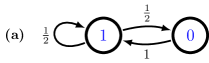
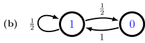
Figure 1: (a) An irreducible Markov chain $M$ of the Golden Mean Process, which consists of all binary sequences with no consecutive $0$s. (b) Its time-reversed chain $\widetilde{M}$ which, in this case, is the same as the original chain.

Every irreducible finite Markov chain has a unique stationary distribution $\pi$ over $\mathcal{A}$ obeying:

$$\pi(y)=\sum_{x\in\mathcal{A}}\pi(x)T(x,y)\quad\text{for all~{}}y\in\mathcal{A}.$$

In matrix notation, we simply write $\pi=\pi T$. The Golden Mean Markov chain has stationary distribution $\pi=(2/3,1/3)$, where $\mathbb{P}(X_{0}=1)=\pi(1)=2/3$.

We calculate the probability of any word ${x}_{0:L}$ by factoring the joint probability $\mathbb{P}({X}_{0:L}={x}_{0:L})$ into a product of conditional probabilities. An application of the Markov property reduces the calculation to:

$$\mathbb{P}(X_{0}=x_{0},X_{1}=x_{1},\ldots,X_{L-1}=x_{L-1})$$

$$=\pi(x_{0})T(x_{0},x_{1})T(x_{1},x_{2})\cdots T(x_{L-2},x_{L-1})$$

$$=\pi(x_{0})\prod_{t=1}^{L-1}T(x_{t-1},x_{t}).$$

More generally, one considers order-$R$ Markov processes for which the next symbol depends on the previous $R$ symbols. (See App. A.) Although these can be shown to be equivalent to a standard Markov chain over a larger state space, we avoid this approach and consider the Markov order as a property of the process. When the next symbol depends on the entire past, though, then $R$ is infinite and the Markov chain, in effect, has an infinite number of states. In Sec. IV we show how hidden Markov models can be used to represent many such chains, while utilizing only a finite state space.

III.2 Reversibility

A intuitive definition of a reversible Markov process is that it should be indistinguishable (in probability) from the same process run backwards in time. Thus, we define a Markov process as reversible if and only if for all $w\in\mathcal{A}^{L}$ and all $L\in\mathbb{N}$, we have:

$$\mathbb{P}(X_{0:L}=w)=\mathbb{P}(X_{0:L}=\widetilde{w})~{},$$ (1)

where $w=w_{0}\ldots w_{L-1}$ and $\widetilde{w}=w_{L-1}\ldots w_{0}$ is its reversal.

Given a Markov process, if the transition matrix of its unique chain obeys:

$$\pi(x)T(x,y)=\pi(y)T(y,x),$$ (2)

for all $x,y\in\mathcal{A}$, then we say the Markov chain is in detailed balance. Note that the uniqueness of the chain allows us to associate detailed balance with the Markov process as well. The Markov chain representation of the Golden Mean Process in Fig. 1(a) is in detailed balance.

It turns out that a stationary, finite Markov process is reversible if and only if its Markov chain, as specified by $T$, is detailed balance [9]. To see this in one direction, assume detailed balance, then:

$$\mathbb{P}(X_{0:L}=w) =\pi(w_{0})\prod_{t=1}^{L-1}T(w_{t-1},w_{t})$$

$$=\pi(w_{L-1})\prod_{\mathchoice{\hbox to0.0pt{\hss$\displaystyle{t=L-1}$\hss}}{\hbox to0.0pt{\hss$\textstyle{t=L-1}$\hss}}{\hbox to0.0pt{\hss$\scriptstyle{t=L-1}$\hss}}{\hbox to0.0pt{\hss$\scriptscriptstyle{t=L-1}$\hss}}}^{1}T(w_{t},w_{t-1})$$

$$=\mathbb{P}(X_{0:L}=\widetilde{w})~{}.$$

Conversely, if the Markov process is reversible, then by considering only words of length two we have $\mathbb{P}(X_{0}=x,X_{1}=y)=\mathbb{P}(X_{0}=y,X_{1}=x)$. This is exactly the statement of detailed balance.

Given a Markov chain, we can use the condition for detailed balance to define another chain that generates words with the same probabilities as the original chain, but in reverse order. If $T$ is the state transition matrix of an irreducible Markov chain and $\pi$ is its unique stationary distribution, then its time-reversed Markov chain has state transition matrix given by:

$$\widetilde{T}(x,y) \equiv\mathbb{P}(X_{0}=y|X_{1}=x)$$

$$=\frac{\pi(y)T(y,x)}{\pi(x)}~{}.$$ (3)

It is easy to see that if $\pi$ is stationary for $T$, then it is also stationary for $\widetilde{T}$. Figure 1(b) shows the time-reversed chain for the Golden Mean Process. It is the same as the forward-time chain and, thus, is also in detailed balance.

Considering the time-reversed Markov chain as a generator, we interpret:

$$\pi(x)\widetilde{T}(x,y)\widetilde{T}(y,z)$$

as the generator’s probability of seeing $x$ followed by $y$ followed by $z$. In its local time perspective, we can represent this as $\widetilde{X}_{0:3}=xyz$. By construction, our expectation is that this probability should be equal to the probability (as calculated by the forward generator) of seeing $x$ preceded by $y$ preceded by $z$. That is, $X_{0:3}=zyx$. And so, we can justify the designation of being the time-reversed Markov chain by demonstrating that it does, indeed, generate words in reverse time:

$$\mathbb{P}(\widetilde{X}_{0:L}=w) =\pi(w_{0})\prod_{t=1}^{L-1}\widetilde{T}(w_{t-1},w_{t})$$

$$=\pi(w_{L-1})\prod_{\mathchoice{\hbox to0.0pt{\hss$\displaystyle{t=L-1}$\hss}}{\hbox to0.0pt{\hss$\textstyle{t=L-1}$\hss}}{\hbox to0.0pt{\hss$\scriptstyle{t=L-1}$\hss}}{\hbox to0.0pt{\hss$\scriptscriptstyle{t=L-1}$\hss}}}^{1}T(w_{t},w_{t-1})$$

$$=\mathbb{P}(X_{0:L}=\widetilde{w})~{}.$$

This result provides an alternative characterization of reversibility in Markov processes: A Markov process is reversible if and only if:

$$\mathbb{P}(X_{0:L}=w)=\mathbb{P}(\widetilde{X}_{0:L}=w).$$ (4)

Note that while Eq. (1) is a self-comparison test, Eq. (4) is a comparison between two distinct Markov chains. Also, observe that if a Markov chain is reversible, then $T=\widetilde{T}$, due to detailed balance. Thus, a reversible Markov chain is identical to its time-reversed Markov chain. We return to this point when we define reversibility for hidden Markov models.

What about irreversible Markov processes? A simple example will suffice. Consider the process that generates the periodic sequence $\ldots ABCABCABC\ldots$. Note that the time-reversed Markov chain differs: the forward generator will emit $AB$ but not $BA$, while the reverse generator produces $BA$ but not $AB$.

Finally, we comment briefly on the difference between a Markov process and its associated Markov chain. The Markov process exists in the abstract, describing a measure over bi-infinite strings. The Markov chain is a one-sided generator representation taking the form of a single matrix. Within this class of representations, each stationary and finite Markov process has exactly one finite-state Markov chain. Markov processes can also be represented in another model class—the hidden Markov models—and within that model class, we will see that a given Markov process can have multiple presentations.

IV Generators with Unobservable States

In a similar manner, we now consider models of processes whose states are not directly observable, also known as hidden Markov models. Though rather less well understood than Markov processes, much progress has recently been made; for example, see Ref. [10]. Along the way, we highlight differences between hidden Markov models and Markov chains—differences that force one to consider questions of structure very carefully.

IV.1 Definitions

We begin with a Markov chain $R_{0}R_{1}R_{2}\ldots$ over a finite state set $\mathcal{R}$, the state alphabet. This chain is internal to the hidden Markov model. Then, a finite-state hidden Markov model (HMM) is a sequence of outputs $X_{0}X_{1}X_{2}\ldots$, each taking values from a finite set $\mathcal{A}$ that we now call the output alphabet. The output sequence is generated by the internal Markov chain through a set of transition-output matrices—one matrix for each symbol $x\in\mathcal{A}$. Each matrix element $T_{x}(\alpha,\beta)$ gives the transition from (internal) state $\alpha$ to state $\beta$ on generating output $x\in\mathcal{A}$. That is,

$$T_{x}(\alpha,\beta)\equiv\mathbb{P}(X_{0}=x,R_{1}=\beta|R_{0}=\alpha)~{}.$$

Note that the internal Markov chain’s transition matrix is the marginal distribution over the output symbol:

$$T(\alpha,\beta) =\sum_{\mathchoice{\hbox to0.0pt{\hss$\displaystyle{x\in\mathcal{A}}$\hss}}{\hbox to0.0pt{\hss$\textstyle{x\in\mathcal{A}}$\hss}}{\hbox to0.0pt{\hss$\scriptstyle{x\in\mathcal{A}}$\hss}}{\hbox to0.0pt{\hss$\scriptscriptstyle{x\in\mathcal{A}}$\hss}}}T_{x}(\alpha,\beta)$$

$$=\mathbb{P}(R_{1}=\beta|R_{0}=\alpha)~{}.$$

If, for each $x\in\mathcal{A}$ and $\alpha\in\mathcal{R}$ there exists at most one $\beta\in\mathcal{R}$ such that $T_{x}(\alpha,\beta)>0$, then we say the hidden Markov model is unifilar. An equivalent statement is that the entropy of the next state, conditioned on the current state and symbol, is zero: $H[R_{1}|R_{0},{X}_{0}]=0$.

The hidden aspect of a hidden Markov model refers to the fact that the internal Markov chain is not directly observed—only the sequence of output symbols $X_{0}X_{1}X_{2}\ldots$ is seen. Note, the process associated with a hidden Markov model refers only to the probability distribution $\mathbb{P}(\ldots X_{0}X_{1}X_{2}\ldots)$ over the output symbols ${X}_{t}$ and not over the joint process $(R_{t},X_{t})$.

Non-Markov processes differ from Markov processes in that they exhibit arbitrarily long conditional correlations. That is, the probability of the next symbol may depend on the entire history leading up to this symbol. Due to this, non-Markov processes cannot be represented by finite-state Markov chains. One signature of (and motivation for) hidden Markov models is that they can represent many non-Markov processes finitely. So, whenever a process (Markov or not) has a finite-state hidden Markov model presentation, then we say that the process is finite.

There are a number of hidden Markov model variants. One common variant is a state-emitting hidden Markov model [11]. Another variant is an edge-emitting hidden Markov model. State-emitting hidden Markov models output symbols during state visitations, while edge-emitting hidden Markov models output symbols on the transitions between states. The two variants are equivalent [4] in that they represent the same class of processes finitely. In the following, we always refer to the edge-emitting variant.

As before, we restrict our attention to hidden Markov models whose underlying Markov chain is irreducible. Thus, a hidden Markov model has a unique stationary distribution $\pi$ satisfying $\pi=\pi\sum T_{x}=\pi T$ and, for $\alpha\in\mathcal{R}$, $\pi(\alpha)$ represents the stationary probability of being in internal state $\alpha$.

For comparison, Fig. 2(a) displays a hidden Markov model for the Golden Mean Process. The internal state set is $\mathcal{R}=\{A,B\}$ and the output alphabet is $\mathcal{A}=\{0,1\}$. The transitions between the states sport the labels $p|{\color[rgb]{0,0,1}x}$, where $p=T_{x}(\alpha,\beta)$.

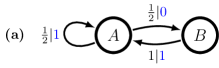
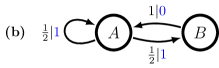
Figure 2: (a) The Golden Mean Process as a hidden Markov model. The internal state set is $\mathcal{R}=\{A,B\}$ and the observation alphabet is $\mathcal{A}=\{0,1\}$. The transitions between states specify $p|{\color[rgb]{0,0,1}x}$ where $p=\mathbb{P}(X_{0}=x,R_{1}=\beta|R_{0}=\alpha)$. (b) Its time-reversed hidden Markov model is not the same. It is nonunifilar, while the forward presentation is.

The probability of any word is calculated as:

$$\mathbb{P}(X_{0}=x_{0},\ldots,X_{L-1}=x_{L-1})$$

$$=\sum_{\mathchoice{\hbox to0.0pt{\hss$\displaystyle{\rho_{0},\ldots,\rho_{L}}$\hss}}{\hbox to0.0pt{\hss$\textstyle{\rho_{0},\ldots,\rho_{L}}$\hss}}{\hbox to0.0pt{\hss$\scriptstyle{\rho_{0},\ldots,\rho_{L}}$\hss}}{\hbox to0.0pt{\hss$\scriptscriptstyle{\rho_{0},\ldots,\rho_{L}}$\hss}}}\pi(\rho_{0})T_{x_{0}}(\rho_{0},\rho_{1})\cdots T_{x_{L-1}}(\rho_{L-1},\rho_{L}).$$

In matrix form, with $T_{w}\equiv T_{w_{0}}\cdots T_{w_{L-1}}$, we have

$$\mathbb{P}(X_{0:L}=w)=\pi T_{w}\mathbf{1},$$

where $\mathbf{1}=(11\ldots 11)^{t}$.

The states $\mathcal{R}$ and observations $\mathcal{A}$ were synonymous in Markov chains. The consequence of this was that every finite Markov process was uniquely characterized by its transition matrix $T$. With hidden Markov models, this is no longer true. A given process, even a Markov process, is not uniquely characterized by a set of transition matrices $\{T_{x}\}$. To drive this point home, Sec. V provides an example process that has an uncountable number of presentations on a fixed, finite number of states. This demonstrates the need for a canonical representation, which is also introduced in Sec. V.

IV.2 Reversibility

In comparison to Markov chains, the literature on reversibility for hidden Markov models is substantially smaller and not nearly as detailed—see, for example, Ref. [12].

Reversibility for Markov processes was defined, in Eq. (1), such that the probability of every word equaled the probability of the reversed word. We take this as a general definition, applicable even to non-Markov processes. Thus, a process is reversible if and only if for all $w\in\mathcal{A}^{L}$ and all $L\in\mathbb{N}$, we have:

$$\mathbb{P}(X_{0:L}=w)=\mathbb{P}(X_{0:L}=\widetilde{w}),$$ (5)

where, as before, $\widetilde{w}$ is the reversal of $w$.

Detailed balance plays a central role in Markov chains and their applications. The analogous local-equilibrium property for hidden Markov models is more subtle and interesting. We define detailed balance for a hidden Markov model to mean that the following must hold for all $x\in\mathcal{A}$ and all $\alpha,\beta\in\mathcal{R}$:

$$\pi(\alpha)T_{x}(\alpha,\beta)=\pi(\beta)T_{x}(\beta,\alpha)~{}.$$ (6)

Trivially, if a hidden Markov model is in detailed balance, then its internal Markov chain must also be in detailed balance. The converse, however, is not true. Also, whenever a hidden Markov model is in detailed balance, one can show that the process it generates is reversible. But unlike the Markov chain case, detailed balance is not equivalent to reversibility. And, quite generally, the process generated by a hidden Markov model can be reversible even if the model is not in detailed balance . The Golden Mean Process of Fig. 2(a) generates a reversible process, but it is not in detailed balance. The contrapositive is perhaps more intriguing: Every irreversible stationary process generated by a finite-state, edge-emitting hidden Markov model is not in detailed balance .

We can use the condition of detailed balance to inspire a definition for the time-reversed hidden Markov model. If $T_{x}$ are the labeled transition matrices of a hidden Markov model and $\pi$ is its unique stationary distribution, then its time-reversed hidden Markov model has labeled transition matrices given by:

$$\widetilde{T}_{x}(\alpha,\beta) \equiv\mathbb{P}(X_{0}=x,R_{0}=\beta\,|\,R_{1}=\alpha)$$

$$=\frac{\pi(\beta)T_{x}(\beta,\alpha)}{\pi(\alpha)}~{}.$$ (7)

The time-reversed HMM for the Golden Mean Process is given in Fig. 2(b), which is now nonunifilar.

As before, if $\pi$ is stationary for $T=\sum T_{x}$, then it is also stationary for $\widetilde{T}=\sum\widetilde{T}_{x}$. To justify its designation as the time-reversed hidden Markov model, we demonstrate that it does indeed generate words in reverse time and, thus, generates the time-reversed process:

$$\mathbb{P}(\widetilde{X}_{0}=x_{0},\ldots,\widetilde{X}_{L-1}=x_{L-1})$$

$$=\sum_{\mathchoice{\hbox to0.0pt{\hss$\displaystyle{\rho_{0},\ldots,\rho_{L}}$\hss}}{\hbox to0.0pt{\hss$\textstyle{\rho_{0},\ldots,\rho_{L}}$\hss}}{\hbox to0.0pt{\hss$\scriptstyle{\rho_{0},\ldots,\rho_{L}}$\hss}}{\hbox to0.0pt{\hss$\scriptscriptstyle{\rho_{0},\ldots,\rho_{L}}$\hss}}}\pi(\rho_{0})\widetilde{T}_{x_{0}}(\rho_{0},\rho_{1})\cdots\widetilde{T}_{x_{L-1}}(\rho_{L-1},\rho_{L})$$

$$=\sum_{\mathchoice{\hbox to0.0pt{\hss$\displaystyle{\rho_{0},\ldots,\rho_{L}}$\hss}}{\hbox to0.0pt{\hss$\textstyle{\rho_{0},\ldots,\rho_{L}}$\hss}}{\hbox to0.0pt{\hss$\scriptstyle{\rho_{0},\ldots,\rho_{L}}$\hss}}{\hbox to0.0pt{\hss$\scriptscriptstyle{\rho_{0},\ldots,\rho_{L}}$\hss}}}\pi(\rho_{L})T_{x_{L-1}}(\rho_{L},\rho_{L-1})\cdots T_{x_{0}}(\rho_{1},\rho_{0})$$

$$=\mathbb{P}(X_{0}=x_{L-1},\ldots,X_{L-1}=x_{0})~{}.$$

This result provides an alternative characterization of reversibility which parallels that for Markov chains given in Eq. (4). That is, a hidden Markov model is reversible if and only if for all $w\in\mathcal{A}^{L}$ and all $L\in\mathbb{N}$, we have:

$$\mathbb{P}(X_{0:L}=w)=\mathbb{P}(\widetilde{X}_{0:L}=w),$$ (8)

indicating that the two hidden Markov models agree on the probability of every word; cf. Eq. (5). Also, note that if the hidden Markov model is in detailed balance, then it equals the time-reversed hidden Markov model: $T_{x}=\widetilde{T}_{x}$. We see that detailed balance is a structurally restrictive property.

For Markov chains, determining if a process is reversible amounted to checking for detailed balance. The situation is more complicated for hidden Markov models but, curiously enough, there exists a straightforward procedure to check if two hidden Markov models generate the same process language. This is known as the identifiability problem [15], and its solution [16, 17, 4], though 20 years old now, does not seem to be as well known. A crude test is to verify that the hidden Markov model and its time-reversed hidden Markov model agree on the probabilities of every word of length $L$, where $L<2|\mathcal{R}|$ and $|\mathcal{R}|$ is the number of states in the model [4].

Another interesting question is whether or not the reversibility of the internal Markov chain has any effect on the reversibility of the observed process. As it turns out, the answer is no. Jumping ahead a bit, we note that the forward $\epsilon$-machine in Fig. 9 has a reversible internal Markov chain, but the observed process is irreversible. Additionally, to any irreversible Markov chain, we can simply assign the same symbol on each outgoing edge. This creates a period-$1$ process that is definitely reversible. So, the reversibility of the internal Markov chain can make no statement on the reversibility of the observed process.

V Structure and Canonical Presentations

Rarely does one work directly with a process. Needless to say, specifying the probability of every word at every length is a cumbersome representation. Instead, one works with generators. However, one must be careful in choosing a representation for the latter. For example, the class of processes representable by finite-state hidden Markov models is strictly larger than the class of processes representable by finite-state Markov chains [18]. So, one cannot use Markov chain presentations in many cases.

As previously noted, when the process can be represented by a finite-state Markov chain, then that presentation is unique. If the process has no finite-state Markov chain representation, however, then there is a challenging multiplicity of possible hidden Markov model presentations to choose from, many with distinct structural properties. As an example, Fig. 3 gives a continuously parametrized set hidden Markov models for the Golden Mean Process. Each value of $z=\mathbb{P}(B,0|A)\in[\frac{1}{2},1]$ defines a unique hidden Markov model that generates the same Golden Mean Process. That is, $\mathbb{P}(X_{1}=\beta|X_{0}=\alpha)$ is independent of $z$ and equal to the matrix $T(\alpha,\beta)$ that defined the Markov chain in Fig. 1(a). Note that this is only a two-state hidden Markov model. It is possible to construct similar families with even more states. (The technique for constructing such continuously parametrized presentations for a given process will appear elsewhere.)

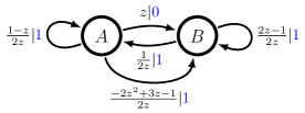
Figure 3: The Golden Mean Process as a continuously parametrized hidden Markov model. The internal state set is $\mathcal{R}=\{A,B\}$ and the observation alphabet is $\mathcal{A}=\{0,1\}$. Each value of $z=\mathbb{P}(B,0|A)\in[\frac{1}{2},1]$ defines a unique hidden Markov model that generates the same process as the models in Figs. 1(a) and 2(a).

This degeneracy serves to emphasize why a process’s structure and that of its presentations deserve close attention. To appreciate this concern more deeply, we detour and examine structure explicitly. Then, we introduce $\epsilon$-machines and show how they provide a canonical presentation that, in addition to other benefits, resolves the degeneracy. Finally, we discuss additional notions of reversibility that are more closely tied to and calculable from $\epsilon$-machines.

V.1 Decomposing the State

Reference [3] presented an information-theoretic analysis of the relationship between a hidden Markov model’s states and the process it generates. One of the main conclusions was that the internal-state uncertainty $H[R_{0}]$ can be decomposed into four independent components. Here, we summarize the decomposition, assuming a minimal amount of information theory. Reference [19] should be consulted for background not covered here. Familiarity with the block entropy, entropy rate, and excess entropy as developed in Ref. [3] is also assumed.

By splitting a process’s bi-infinite sequence of random variables into a past $X_{:0}$ and a future $X_{0:}$, we isolate the information that passes through the present state $R_{0}$. As developed in Refs. [20] and [21], the statistical relationships among these three (aggregate) variables are concisely expressed using the information diagram technique of Refs. [22] and [23]. Said briefly, a process’s Shannon entropies and mutual informations [24] form a measure over the associated event (sequence) spaces. Given this, the set-theoretic relationships between the measure’s atoms are displayed in the Venn-like diagram.

For a three-variable information diagram, we have three circles representing $H[X_{:0}]$, $H[X_{0:}]$, and $H[R_{0}]$. In total, this means that there are $7$ atoms to consider. However, since every hidden Markov model has an internal Markov chain that governs generation, the past and future are shielded from each other given the current state. This is a probabilistic statement, but when phrased in terms of conditional mutual information, we have $I[X_{:0};X_{0:}|R_{0}]=0$. A moment’s reflection shows that this is a way of saying that the hidden Markov model generates the process. This quantity can be nonzero only if we compare a process to the states of a hidden Markov model that generates a different process.

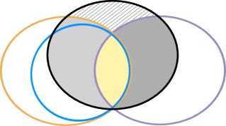
Figure 4: Information diagram capturing all possible relationships between the past $X_{:0}$, the future $X_{0:}$, and the present—the current internal state $R_{0}$. The statistical complexity $C_{\mu}$, excess entropy ${\bf E}$, crypticity $\chi$, oracular information $\zeta$, and gauge information $\varphi$ appear as unions and intersections of the resulting atoms.

The information diagram is shown in Fig. 4. There, $H[X_{:0}]$ is represented by everything contained in the orange circle . The purple circle represents $H[X_{0:}]$ and the black circle, our focus, represents state information $H[R_{0}]$. The figure contains an additional blue circle that can be ignored until $\epsilon$-machines are introduced in Sec. V.2. So, absent the blue circle, we see that the state information decomposes into four quantities. Specifically,

$$H[R_{0}]={\bf E}+\chi+\zeta+\varphi~{},$$ (9)

where we have the:

1. Excess entropy: ${\bf E}=I[X_{:0};X_{0:}]$,

2. Crypticity: $\chi=I[X_{:0};R_{0}|X_{0:}]$,

3. Oracular information: $\zeta=I[R_{0};X_{0:}|X_{:0}]$, and

4. Gauge information: $\varphi=H[R_{0}|X_{:0},X_{0:}]$.

Excess entropy is a by-now standard measure of complexity [26, 27, 28, 29, 30] that captures the shared information between past and future observations. Crypticity is a relatively new measure of structure introduced in Refs. [20, 21, 31]. By comparing to the apparent information that excess entropy measures, crypticity monitors how much of the internal state information is hidden. Oracular information, introduced in Ref. [3], measures how much information a presentation provides that can improve predictability, but that is not available from the past. Finally, gauge information, also introduced in Ref. [3], quantifies how much additional structural information exists in a presentation that is not “justified” by the past or the future. Taken together these quantities provide an informational basis useful for analyzing the various kinds of structure a process or a process’s presentation contains.

To see this, we can apply these structural complexity measures to the Golden Mean Process presentation family of Fig. 3. For each value of $z=\mathbb{P}(B,0|A)\in[\frac{1}{2},1]$, Fig. 5 plots ${\bf E}$, $\chi$, $\zeta$, and $\varphi$ stacked in way so that their sum $H[R_{0}]$ is the top curve. One immediately sees that ${\bf E}$ is independent of $z$. This is as it should be since ${\bf E}$ is a function only of the observed process and, by construction, the parametrized presentation always generates the Golden Mean Process. All of the other measures change as the presentation changes, however. Let’s explore what they tell us.

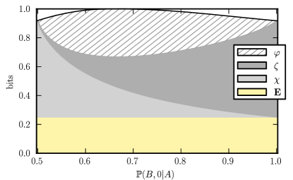
Figure 5: Decomposition of the state information $H[R]$ contained in the parametrized Golden Mean Process presentation family of Fig. 3. As a function of $z=\mathbb{P}(B,0|A)\in[\frac{1}{2},1]$, the excess entropy ${\bf E}$, crypticity $\chi$, oracular information $\zeta$, and gauge information $\varphi$ are stacked such that the top of the curve is their sum $H[R]$, the state entropy of the presentation for the given value of $z$. The miniaturized information diagrams are special cases of Fig. 4 tailored to $z$-values. From left-to-right, we have $z=\frac{1}{2}$, $z=\frac{3}{4}$, and $z=1$.

Beginning with $z=1/2$, we recover the Markov chain presentation of Fig. 2(a). In this presentation, all of the state information $H[R_{0}]$ is contained within $H[X_{:0}]$. This is represented by the leftmost information diagram at the top of Fig. 5. Loosely, we say that the state information contains only information from the past. However, one must keep in mind that the presentation still captures ${\bf E}$ bits of information, and this information is shared with the future. The gauge and oracular informations vanish. It turns out that the $z=1/2$ presentation is the process’s forward $\epsilon$-machine, but more on this later.

As $z$ increases, so do the gauge and oracular informations. With this change, the information diagram circle for $H[R_{0}]$ straddles $H[X_{:0}]$ and $H[X_{0:}]$, as shown in the central information diagram atop Fig. 5. This indicates that the state information now consists of historical information, oracular information, and also gauge information. For all values of $z$, the overlap that $H[R_{0}]$ has with the intersection of the past and future is constant. This is because each presentation generates the process and so each must capture ${\bf E}$ bits of shared information.

Finally when $z=1$, the circle for $H[R_{0}]$ is now completely contained inside the future $H[X_{0:}]$. Now, the information diagram resembles the right-most one atop Fig. 5. There is no crypticity, no gauge information, but there is oracular information. The interpretation is that the state information, apart from ${\bf E}$, consists only of information from the future. As we will see, the $z=1$ presentation corresponds to the time-reversed presentation of the reverse $\epsilon$-machine. And, since the Golden Mean Process is a reversible Markov chain, the $z=1$ information diagram mirrors the diagram for $z=\frac{1}{2}$.

V.2 $\epsilon$-Machines

We discussed processes in the context of generators, as represented by Markov chains and hidden Markov models, but another important aspect concerns prediction. As we will show, $\epsilon$-machines are a natural consequence of this perspective, and they provide a much richer analysis of irreversibility. Additionally, their uniqueness provides a solution to the multiplicity of HMM presentations.

Consider again a process’s output sequence and, now, interpret time as increasing with the index. The result is a time-series $\ldots{X}_{t-1}{X}_{t}{X}_{t+1}\ldots$. Our goal is to construct a model that predicts future observations. Specifically, we want to find sufficient statistics that preserve our ability to predict. Translating this into a concrete procedure, we first remove redundancies in the time-series, by grouping histories that lead to the same distribution over futures:

$${x}_{:0}\sim{x}_{:0}^{\prime}\iff\mathbb{P}(X_{0:}|X_{:0}={x}_{:0})=\mathbb{P}(X_{0:}|X_{:0}={x}_{:0}^{\prime})~{}.$$

The grouping defines an equivalence relation over histories and, thus, partitions the space of histories. This partition is the coarsest one that provides optimal prediction. It is called the process’s causal state partition. Each equivalence class is known as a causal state and, thus, to each causal state, there is a unique distribution over futures [32, 8, 33]. The set of causal states is denoted $\bm{\mathcal{S}}$.

Now, consider a semi-infinite history $X_{:0}=x_{:0}$ which, by the causal state equivalence relation, induces causal state $\mathcal{S}_{0}=\sigma_{0}$. If we append a new observation, we get $X_{:1}=x_{:0}x_{0}$ which, in turn, induces $\mathcal{S}_{1}=\sigma_{1}$. In this sense, there is a natural dynamic over the causal states that is induced by the dynamic over the observed sequences. This dynamic is represented in Fig. 6. The pair of causal states and transition dynamic is called a process’s $\epsilon$-machine.

Figure 6: The dynamic over the causal states is induced by the dynamic over the (semi-infinite) histories. For example, a history ${X}_{-1:}$ ending at $t=-1$, maps to causal state $\mathcal{S}_{0}$. When a new symbol $X_{0}$ is appended to the old history, we induce a new causal state $\mathcal{S}_{1}$.

Generally, the set of causal states can be uncountable, countable, or finite; see, for example, Fig. 17 in Ref. [8]. Even when the set is not finite, the set that is visited infinitely often may be finite. The infinitely visited subset defines the recurrent causal states. All other states are transient causal states and not the subject of our discussion here. Now, when the set of recurrent causal states is finite, then the $\epsilon$-machine—obtained by partitioning histories for the purposes of prediction—is representable as a finite-state unifilar hidden Markov model. We denote the transition matrices in the same way, except that we use $\mathcal{S}$ as the state random variables, which take on values from $\bm{\mathcal{S}}$:

$$T_{x}(\alpha,\beta)=\mathbb{P}({X}_{0}=x,\mathcal{S}_{1}=\beta|\mathcal{S}_{0}=\alpha)~{}.$$

$\epsilon$-Machines with a finite number of recurrent states generate a subset of the finitary processes—processes with finite excess entropy. This subset represents a strictly larger set of processes than finite-state Markov chains since it includes processes with measures over strictly sofic [34] shifts.

The $\epsilon$-machine is the unique presentation in the class of unifilar hidden Markov models [32, 33] and, thus, it defines a canonical presentation for a given process. There are other benefits. For one, $\epsilon$-machine unifilarity allows one to directly calculate the process entropy rate. Early on, Shannon pointed out that this is always possible to do with Markov chains. It was soon discovered that it is not possible using nonunifilar hidden Markov models [15]. Nonunifilarity makes each presentation state appear more random than it actually is. For a more detailed treatment of $\epsilon$-machines, see Ref. [32].

We pause briefly to point out that the unifilarity property of the $\epsilon$-machine is a consequence of the equivalence relation. It has been known for some time [8, 21, 35] that there are nonunifilar hidden Markov models of processes that can be smaller, sometimes substantially smaller, than the process’s $\epsilon$-machine. However, finding a canonical presentation within the class of nonunifilar hidden Markov models is a task that has evaded solution. One obvious choice is to focus on the hidden Markov model that minimizes the state entropy; see Ref. [35] for further discussion. Since our goal is to analyze the role that structure plays in irreversibility, having a canonical representation is essential. So, our focus on $\epsilon$-machines is based, in part, on practicality since one can calculate the $\epsilon$-machine from any alternative presentation. It is also theoretically useful since many quantities—such as the process entropy rate and excess entropy—are not exactly calculable from nonunifilar presentations. Additionally, the states of nonunifilar presentations are not sufficient statistics for the histories. The consequence is that one cannot forget the past and work with an individual state in a general hidden Markov model—instead, one must work with a distribution over the states .

Our discussion of processes began by pointing out that time is merely an interpretation of the indices on a set of random variables. Thus far, we described $\epsilon$-machines from the forward perspective—yielding the forward $\epsilon$-machine, denoted ${M}^{+}$. Similarly, following Refs. [20, 21] one can partition futures for the purposes of retrodiction, and this partitioning induces a dynamic over the reverse causal states. The resulting unifilar hidden Markov model is known as the reverse $\epsilon$-machine, denoted ${M}^{-}$. To differentiate the states in each hidden Markov model, we let ${\mathcal{S}}^{+}_{t}$ represent the random variables for the forward causal states and use ${\mathcal{S}}^{-}_{t}$ for the reverse causal states. The equivalence relations used during partitioning, $\sim^{+}$ and $\sim^{-}$, are generally distinct. We use $\epsilon^{+}:\smash{\overleftarrow{{x}}}\to{\mathcal{S}}^{+}$ to denote the mapping that takes a history and returns the forward causal state into which the history was partitioned. Similarly, we use $\epsilon^{-}:\smash{\overrightarrow{{x}}}\to{\mathcal{S}}^{-}$ to denote the mapping from futures to reverse causal states.

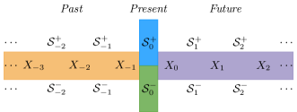
Figure 7: Hidden Process Lattice: The ${X}$ variables denote the observed process; the $\mathcal{S}$ variables, the hidden causal states. If one scans the observed variables in the positive direction—seeing ${X}_{-3}$, ${X}_{-2}$, and ${X}_{-1}$—then that history takes one to causal state ${\mathcal{S}}^{+}_{0}$. Analogously, if one scans in the reverse direction, then the succession of variables ${X}_{2}$, ${X}_{1}$, and ${X}_{0}$ leads to ${\mathcal{S}}^{-}_{0}$. The colors indicate which variables participate in the information measures of Fig. 8.

To orient ourselves, Fig. 7 places the relevant random variables on a lattice. The ${X}$ variables denote the observed process of the hidden Markov model, which is broken up into the past (orange) and future (purple) observation sequences. The hidden causal states are represented by the $\mathcal{S}$ variables. In the present, we have ${\mathcal{S}}^{+}_{0}$ and ${\mathcal{S}}^{-}_{0}$ straddling the past and future. If one scans the observed variables in the positive direction—seeing ${X}_{-3}$, ${X}_{-2}$, and ${X}_{-1}$—then that history takes one to causal state ${\mathcal{S}}^{+}_{0}$. Analogously, if one scans in the reverse direction, then the succession of variables ${X}_{2}$, ${X}_{1}$, and ${X}_{0}$ leads to ${\mathcal{S}}^{-}_{0}$.

Summarizing, we represent each $\epsilon$-machine as a commuting diagram that operates on the hidden process lattice, using $x$ and $\sigma$ to represent symbol and causal state realizations, respectively:

For the forward $\epsilon$-machine $M^{+}$, every past ${x}_{:0}$ maps to a unique next past ${x}_{:1}$ on symbol ${x}_{0}$. By the forward-looking map $\epsilon^{+}$, each past ${x}_{:0}$ corresponds to unique causal state $\sigma^{+}_{0}$. This many-to-one correspondence induces a dynamic on the causal states such that $\sigma^{+}_{0}$ transitions to $\sigma^{+}_{1}$ on symbol ${x}_{0}$. Similarly, for the reverse $\epsilon$-machine ${M}^{-}$, every future ${x}_{1:}$ maps to a unique next future ${x}_{0:}$ on symbol ${x}_{0}$. The reverse-looking map $\epsilon^{-}$ associates ${x}_{1:}$ with $\sigma^{-}_{1}$. The many-to-one correspondence induces a dynamic on the reverse causal states such that $\sigma^{-}_{1}$ transitions to $\sigma^{-}_{0}$ on symbol ${x}_{0}$.

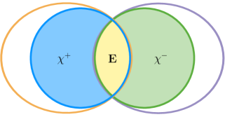
Figure 8: Information diagram for the forward and reverse $\epsilon$-machines.

Finally, we gather the forward and reverse $\epsilon$-machines in Fig. 8. Together, they provide complementary views of the process. For example, the minimal amount of information one must store in order to generate the process in the forward direction defines the forward statistical complexity $C_{\mu}^{+}\equiv H[{\mathcal{S}}^{+}]$. This information, in general, is not equal to the minimal amount of information one requires for retrodiction $C_{\mu}^{-}\equiv H[{\mathcal{S}}^{-}]$ [20, 21, 31]. Notably, the $\epsilon$-machine has no gauge information since it is minimal and, also, no oracular information since it is unifilar. Referring briefly back to Figs. 4 and 5, when $z=\frac{1}{2}$, we have the forward $\epsilon$-machine. When $z=1$, we have the time-reversed presentation of the reverse $\epsilon$-machine $\widetilde{M}^{-}$. The interpretation is direct: The crypticity $\chi^{-}$ of the reverse $\epsilon$-machine becomes oracular information $\zeta$ in the time-reversed presentation.

Our preference, from now on, is to use the forward and reverse $\epsilon$-machines. Given the forward $\epsilon$-machine $M^{+}$, we can construct, via Eq. (7), a reverse generator of the process $\widetilde{M}^{+}$. However, this is just one presentation among many possible reverse generators of the process. So, we operate on that reverse generator, using techniques from Ref. [21], and obtain the reverse $\epsilon$-machine $M^{-}$. Together, the forward and reverse $\epsilon$-machines serve as the basis for understanding processes through the use of generators. In Sec. VII, we unify the two $\epsilon$-machines into a single machine and discuss its meaning in the context of the decomposition of state information.

V.3 Finite State Automata

One interesting property of $\epsilon$-machines, and hidden Markov models in general, is that they are intimately related to automata in formal language theory [37]. Here, we briefly review their relationship.

Given a process $\mathcal{P}$, we can examine the set of all words that occur with positive probability. This set is known as the support of the process’s stochastic language. Stripping away the transition probabilities of any finite-state hidden Markov model leaves a finite-state automaton that generates the support of the process language. So, we see that the support of a process generated by finite-state HMM always corresponds to a regular language. If the hidden Markov model was unifilar, then the resulting structure, without probabilities, is equivalent to a deterministic finite automata (DFA). Similarly, nonunifilar hidden Markov models map to nondeterministic finite automata (NFA).

However, it is necessary to point out that there are quite drastic differences between formal and process languages. While DFAs and NFAs are equivalent in the set of formal languages that each can represent using a finite number of states, the same is not true of hidden Markov models. In fact, there are finite-state nonunifilar HMMs that have no corresponding finite-state unifilar counterpart. One well known example is the Simple Nondeterministic Source of Ref. [8]. It can be represented as a two-state nonunifilar HMM, but its $\epsilon$-machine—the smallest unifilar HMM generating the same process—requires a countably infinite number of states.

Since it will be useful to compare topological properties to statistical properties, we define $M_{\emptyset}^{+}$ and $M_{\emptyset}^{-}$ as the deterministic finite-state automata corresponding to the forward and reverse $\epsilon$-machines with all probabilities removed. Note that these DFAs need not be the minimal deterministic finite-state automata [37] generating the support, and this fact highlights the difference between the causal-state equivalence relation and the Nerode state-equivalence relation in formal language theory. If we subsequently minimize $M_{\emptyset}^{+}$ and $M_{\emptyset}^{-}$, we are left with the minimal and unique DFAs that generate the support, respectively denoted $D^{+}$ and $D^{-}$.

Also, we mention that there is a large body of literature in formal language theory concerning $k$-reversible languages [38, 39, 40, 41, 42]. This topic does not relate directly to our notion of reversibility and is rather closer to addressing a process’s Markov order; cf. Ref. [43].

One can view $\epsilon$-machines as probabilistic counterparts to DFAs. In fact, the relation between formal language theory and stochastic languages can be extended. Just as there is a hierarchy of models in formal language theory, one can consider a hierarchy of stochastic models as well. See, for example, the process hierarchy proposed in Ref. [8].

V.4 Reversibility Revisited

By focusing on $\epsilon$-machines, we side-step the representational degeneracy of hidden Markov models. Recalling the uniqueness of the forward and reverse $\epsilon$-machines, we note that properties of the $\epsilon$-machine can also be interpreted as properties of the process. This also allows us to consider additional measures of reversibility that are based on structural properties of the $\epsilon$-machine. So, while each of the forthcoming definitions can be stated strictly in terms of the process’s probability distribution, we prefer to use equivalent definitions in terms of the forward and reverse $\epsilon$-machines. This is akin to studying formal languages through the use of the minimal DFAs.

As Ref. [4] demonstrated, there is a finite procedure for determining whether two finite-state hidden Markov models generate the same process language. By Eq. (8), this technique also provides a method for determining whether a process is reversible or not. An alternate technique involves the forward and reverse $\epsilon$-machines. With them, one simply asks if the two machines are identical to each other. If so, then the process is reversible. In Ref. [21], this property was termed microscopic reversibility and we write: $M^{+}=M^{-}$.

We can also consider several weaker forms of reversibility. For example, as we noted, the process that repeats $ABC\ldots$ indefinitely is not reversible, but the $\epsilon$-machines are essentially the same in that the amount of information one requires for prediction equals the amount required for retrodiction. Following Ref. [21], a process is causally reversible if and only if $C_{\mu}^{+}=C_{\mu}^{-}$.

In terms of topology, we say that a process is support reversible if and only if $D^{+}=D^{-}$, where equality means that DFAs must be identical under an isomorphism over the states. Finally, we also consider symbol isomorphisms. If there exists an isomorphism from the output alphabet of ${M}^{+}$ to the output alphabet of ${M}^{-}$ that renders the two machines equal, then we say that the process is reversible under symbol isomorphism, denoted ${M}^{+}\cong{M}^{-}$. Similarly, the process is support reversible under symbol isomorphism if and only if $D^{+}\cong D^{-}$.

VI Examples

This section exercises the preceding theory, giving a number of additional results and illustrating them through example processes and presentations. We start with an exploration of which kinds of reversibility there can be. Then we analyze in detail two example irreversible processes, one with a rather counterintuitive property. The analyses give a concrete understanding of how irreversibility arises and what its structural consequences are for a process. The section closes with a survey that demonstrates the dominance of irreversibility among processes.

VI.1 Causal Reversibility Roadmap

Given these various notions of reversibility, a natural question comes to mind: What combinations are possible? To this end, we state a number of straightforward relationships:

$${M}^{+}={M}^{-}\quad \Rightarrow\quad C_{\mu}^{+}=C_{\mu}^{-}$$ (10)

$${M}^{+}={M}^{-}\quad \Rightarrow\quad D^{+}=D^{-}$$ (11)

$${M}^{+}={M}^{-}\quad \Rightarrow\quad{M}^{+}\cong{M}^{-}$$ (12)

$${M}^{+}\cong{M}^{-}\quad \Rightarrow\quad D^{+}\cong D^{-}$$ (13)

$$D^{+}=D^{-}\quad \Rightarrow\quad D^{+}\cong D^{-}$$ (14)

Now, let us restrict attention to just the causally reversible processes ($C_{\mu}^{+}=C_{\mu}^{-}$) and examine microscopic and support reversibility, with and without symbol isomorphisms. That is, we consider the combinations of the four properties (i) ${M}^{+}={M}^{-}$, (ii) ${M}^{+}\cong{M}^{-}$, (iii) $D^{+}=D^{-}$, and (iv) $D^{+}\cong D^{-}$. Of the $16$ possible Boolean-vector combinations, only $6$ are possible due Eqs. (10) - (14).

$M^{+}\vphantom{M^{M^{M}}_{M_{M}}}$	$M^{-}\vphantom{M^{M^{M}}_{M_{M}}}$	${M}^{+}={M}^{-}\vphantom{M^{M^{M}}_{M_{M}}}$	${M}^{+}\cong{M}^{-}\vphantom{M^{M^{M}}_{M_{M}}}$	$D^{+}=D^{-}\vphantom{M^{M^{M}}_{M_{M}}}$	$D^{+}\cong D^{-}\vphantom{M^{M^{M}}_{M_{M}}}$
		F	F	F	F
		F	F	F	T
		F	F	T	T
		F	T	F	T
		F	T	T	T
		T	T	T	T

Table 1: Diversity of causally reversible processes ($C_{\mu}^{+}=C_{\mu}^{-}$): Example presentations for forward and reverse $\epsilon$-machine pairs, with the same number of states, for the $6$ possible combinations; all other combinations are impossible.

Table 1 gives example forward and reverse $\epsilon$-machine pairs for each of the $6$ possibilities. What we learn from these examples is that causal reversibility indeed captures a larger class of processes than microscopic reversibility. However, it also captures a bit more, including processes that are not isomorphic to one another under a symbol isomorphism. The table also demonstrates that irreversibility is not only a topological concern—the forward and reverse DFAs can be identical while the generated process languages are not.

VI.2 Causal Irreversibility

Irreversible processes are ubiquitous, even among those represented by finite-state $\epsilon$-machines. In our first example, we ground intuitions with a process whose irreversibility is driven topologically. The example is particularly illustrative since its $\epsilon$-machines have a finite number of causal states. In the second example, we examine an irreversible process whose forward and reverse DFAs are identical; this demonstrates that irreversibility can arise purely probabilistically. Then, in the third example, we see the extent to which probability aggravates irreversibility when it causes a finite-state forward $\epsilon$-machine to become an infinite-state reverse $\epsilon$-machine.

VI.2.1 Support-Driven Irreversibility

The first example we consider shows that a process can have different, but finite, numbers of forward and reverse causal states. Formally, Ref. [21] provides the technique for calculating the reverse $\epsilon$-machine via operations on the graph structure of the forward $\epsilon$-machine but, for pedagogical reasons, both the forward and reverse causal states are constructed in terms of $X_{t}$ only .

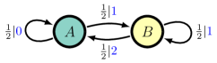
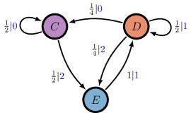
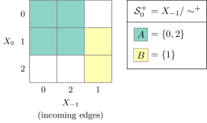
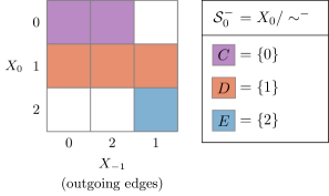
Figure 9: The forward (top left) $M^{+}$ and reverse (bottom left) $M^{-}$ $\epsilon$-machines for a causally irreversible process. Note that $D^{+}\neq D^{-}$ and, thus, $M^{+}\neq M^{-}$. The forward causal states ${\mathcal{S}}^{+}$ (top right) partition all allowable histories $\ldots X_{-1}$. In this example, the states are uniquely characterized by specifying the most recent symbol $X_{-1}$. For example, any valid history ending with a ${\color[rgb]{0,0,1}0}$ or ${\color[rgb]{0,0,1}2}$ maps to state $A$, and the possible futures can begin with a ${\color[rgb]{0,0,1}0}$ or ${\color[rgb]{0,0,1}1}$. The incoming edges of $M^{+}$ correspond to histories ($X_{-1}$), while its outgoing edges correspond to futures ($X_{0}$). The reverse causal states ${\mathcal{S}}^{-}$ (bottom right) partition all allowable futures $X_{0}...$. In this example, the states are uniquely characterized by specifying the earliest symbol of each future. For example, any valid future beginning with a ${\color[rgb]{0,0,1}0}$ maps to state $C$ and the associated histories must end with a ${\color[rgb]{0,0,1}0}$ or ${\color[rgb]{0,0,1}2}$. The incoming edges of $M^{-}$ correspond to futures ($X_{0}$), while its outgoing edges correspond to histories ($X_{-1})$.

Consider the time series over the alphabet $\{0,1,2\}$ whose forward ($M^{+}$) and reverse ($M^{-}$) $\epsilon$-machines are shown in Fig. 9. As we will show, the process language generated by $M^{+}$ is irreversible and, additionally, this irreversibility is due to an underlying topological irreversibility. That is, $D^{+}\neq D^{-}$ implies that ${M}^{+}\neq{M}^{-}$.

To see the topological irreversibility note that in ${M}^{+}$ $w=01$ is a valid word: Start in $A$, see $0$ and stay in $A$, then see $1$ and go to $B$. However, $\widetilde{w}=10$ is not a valid word. We can also see this in a slightly different light by noting that $w$ is valid in ${M}^{+}$, but not valid in ${M}^{-}$.

To understand the forward causal states, consider the distribution of $X_{0}=(0,1,2)$ conditioned on length-$1$ history suffixes:

$$\mathbb{P}(X_{0}|X_{-1}=0) =(1/2,1/2,0),$$

$$\mathbb{P}(X_{0}|X_{-1}=1) =(0,1/2,1/2),~{}\text{and}$$

$$\mathbb{P}(X_{0}|X_{-1}=2) =(1/2,1/2,0).$$

We see that the time series generated by this machine has the following characteristics: Every history that ends on symbol $0$ or $2$, is followed by either $0$ or $1$, with probability $1/2$, but never by symbol $2$. Hence, with regard to the distribution of a one-step future, all histories ending on $0$ or $2$ are equivalent and we denote this class of equivalent histories as causal state $A$. The distribution of symbols following words ending on symbol $1$ is different. They are followed by either symbols $1$ or $2$ with probability $1/2$, but never by symbol $0$. All histories ending in $1$ are hence equivalent with respect to the distribution of a one-step future and we denote their equivalence class as state $B$.

States $A$ and $B$ partition of the entire space of allowable histories. The fact that the equivalence class of a history is determined solely by the last symbol is reflected by the time series of symbols having Markov order $1$. The reader should verify that, in this particular example, Markovity also means that the partition obtained by examining one-step futures is equivalent to the partition obtained by examining arbitrary $L$-step futures. From this, we see that ${\bm{\mathcal{S}}}^{+}=X_{:0}/\sim^{+}$ consists of:

$$A =\{\ldots 0,\>\ldots 2\}~{}\text{and}$$

$$B =\{\ldots 1\},$$

where an ellipsis stands for any valid past.

The partition is represented graphically in the matrix at the top-right of Fig. 9. In it, we independently rearranged the histories and futures so as to cluster the block-structures within the matrix. For each history $X_{-1}$, the distribution over futures $X_{0}$ is (topologically) represented as a column. Histories with the same column colorings belong to the same equivalence class under the forward equivalence relation $\sim^{+}$. Finally, note that the futures are not partitioned by the forward equivalence relation since $X_{0}=1$ is allowable from both $A$ and $B$.

To understand the reverse causal states, we examine the distribution of symbols preceding the future. Since the Markov order does not change when analyzing the time series in the reverse direction (App. A), the equivalence class of a future is determined solely by the first symbol of the future. Additionally, equality of distributions over length-$1$ histories implies equality over arbitrary length-$L$ history distributions. Thus, for $X_{-1}=(0,1,2)$ conditioned on a length-$1$ future, we have:

$$\mathbb{P}(X_{-1}|X_{0}=0) =(1/2,0,1/2),$$

$$\mathbb{P}(X_{-1}|X_{0}=1) =(1/4,1/2,1/4),~{}\text{and}$$

$$\mathbb{P}(X_{-1}|X_{0}=2) =(0,1,0).$$

Any word starting with symbol $0$ can only be preceded by symbols $0$ or $2$ with probability $1/2$ each, but never with symbol $1$. Correspondingly, all futures starting with symbol $0$ are equivalent and their equivalence class is denoted as reverse causal state $C$. Furthermore, any word starting with symbol $1$ is preceded by symbols $0$ or $2$ with probability $1/4$ each or is preceded by symbol $1$ with probability $1/2$. All futures starting with symbol $1$ are equivalent with respect the distribution of preceding symbols and subsumed as reverse causal state $D$. Finally, words starting with symbol $2$ can only be preceded by symbol $1$. The equivalence class of futures starting on symbol $2$ is denoted reverse causal state $E$. From this, we see that ${\bm{\mathcal{S}}}^{-}=X_{0:}/\sim^{-}$ consists of:

$$C =\{0\ldots\},$$

$$D =\{1\ldots\},~{}\text{and}$$

$$E =\{2\ldots\},$$

where an ellipsis now stands for any valid future.

States $C$, $D$, and $E$ partition the space of allowable futures. They are represented in the lower-right matrix of Fig. 9. In it, we rearranged the histories and futures so as to cluster the block-structures within the matrix. For each future $X_{0}$, the distribution over histories $X_{-1}$ is (topologically) represented as a row. Each row coloring is distinct, reflecting the fact that each future belongs to a distinct reverse causal state under the reverse equivalence relation $\sim^{-}$. Finally, note that the histories are not partitioned by the reverse equivalence relation since $X_{-1}=0$, for example, is allowable from both $C$ and $D$.

Note how the space of histories is partitioned into only two equivalence classes, while the space of futures is partitioned into three equivalence classes. Any first-order Markov chain on $k$ symbols has at most $k$ causal states. That we only have two forward causal states is due to the fact that the future distributions after seeing symbols $2$ and $0$ are equivalent. This equivalence, however, does not hold in the reverse direction and, so, there are three reverse causal states. The asymmetry is further exemplified by the forward $\epsilon$-machine having smaller statistical complexity than the reverse $\epsilon$-machine: $C_{\mu}^{+}=1~{}\text{bit}~{}<C_{\mu}^{-}=3/2~{}\text{bit}$. For this particular process, it takes $1/2$ bit more memory, on average, to generate the same string of symbols from right to left than from left to right.

Comparing the causal states as represented in Fig. 9, we see that each equivalence relation also defines a partition over the set $(X_{-1},X_{0})$. This, in turn, extends to a partition over bi-infinite strings. So, we can think of the forward (reverse) $\epsilon$-machine as the restriction of this partition to the set of histories (futures). The partition over the bi-infinite strings must be such that when it is restricted to histories (futures) it induces a unifilar dynamic over equivalence classes. This particular point will be important when we discuss the bidirectional machine in Sec. VII.

VI.2.2 Probability-Driven Irreversibility

In our second example, we show that irreversibility can have purely probabilistic origins. We do this with an irreversible, order-$2$ Markov process that has a reversible support. Figure 10 presents the recurrent components of the forward and reverse $\epsilon$-machines, ${M}^{+}$ and ${M}^{-}$. To see that the support is reversible, note that the $\epsilon$-machine structures, without probabilities, are equal: $M^{+}_{\emptyset}=M^{-}_{\emptyset}$. This implies that $D^{+}=D^{-}$, but it can also be seen directly since the topologies, in this example, are already minimal deterministic finite automata. The practical consequence of having a reversible support is that $\mathbb{P}(w)>0$ if and only if $\mathbb{P}(\widetilde{w})>0$.

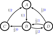
Figure 10: The forward (top) $M^{+}$ and reverse (bottom) $M^{-}$ $\epsilon$-machines of an irreversible, order-$2$ Markov process. The process is irreversible since ${M}^{+}\neq{M}^{-}$. However, the support is reversible since the underlying topologies of each $\epsilon$-machine are the same: $M^{+}_{\emptyset}=M^{-}_{\emptyset}$.

Beginning with the forward causal states, we examine the distribution of symbols that succeed histories. Since the process is order-$2$ Markovian, we calculate finite histories and futures instead of semi-infinite histories and futures. Specifically, partitioning length-$2$ histories based on the conditional distributions of length-$2$ futures yields the same result as partitioning semi-infinite histories based on the conditional distributions of arbitrary length futures . We directly calculate $\mathbb{P}(X_{0},X_{1}|X_{-2},X_{-1})$ as a right-stochastic matrix, finding:

$$\mathbb{P}(X_{0},X_{1}|X_{-2},X_{-1})$$

$$\quad=\bordermatrix{&01&02&10&12&20&21\cr 01&0&1/2&0&0&1/4&1/4\cr 02&0&0&1/2&1/2&0&0\cr 10&0&0&0&0&0&1\cr 12&1/2&0&1/4&1/4&0&0\cr 20&0&0&1/2&1/2&0&0\cr 21&0&1/2&0&0&1/4&1/4}.$$

The forward causal states are groupings of histories and, in this presentation, they correspond to groupings of identical rows. For example, the rows corresponding to $01$ and $21$ are identical and, so, are grouped into the same equivalence class. Translating these history suffixes back into semi-infinite histories, we find that ${\bm{\mathcal{S}}}^{+}=X_{:0}/\sim^{+}$ consists of:

$$A =\{\ldots 02,\>\ldots 20\},$$

$$B =\{\ldots 01,\>\ldots 21\},$$

$$C =\{\ldots 10\},~{}\text{and}$$

$$D =\{\ldots 12\}.$$

The reverse causal states are similarly obtained, but now we consider the distribution of symbols that precede futures. Once again, we work with finite-length histories and futures. Using a right-stochastic matrix, we calculate $\mathbb{P}(X_{-2},X_{-1}|X_{0},X_{1})$ directly as:

$$\mathbb{P}(X_{-2},X_{-1}|X_{0},X_{1})$$

$$\quad=\bordermatrix{&01&02&10&12&20&21\cr 01&0&0&0&1&0&0\cr 02&1/4&0&0&0&0&3/4\cr 10&0&1/2&0&1/4&1/4&0\cr 12&0&1/2&0&1/4&1/4&0\cr 20&1/4&0&0&0&0&3/4\cr 21&1/12&0&2/3&0&0&1/4}.$$

The reverse causal states are groupings of futures, and this corresponds to groupings of identical rows in the matrix. Translating these future prefixes into semi-infinite futures, we find that the reverse causal states ${\bm{\mathcal{S}}}^{-}=X_{0:}/\sim^{-}$ consist of:

$$E =\{02\ldots,\>20\ldots\},$$

$$F =\{10\ldots,\>12\ldots\},$$

$$G =\{01\ldots\},~{}\text{and}$$

$$H =\{21\ldots\}.$$

Since there are multiple perspectives involved, we detour briefly to translate the matrix $\mathbb{P}(X_{-2},X_{-1}|X_{0},X_{1})$ onto the reverse $\epsilon$-machine shown in Fig. 10. One perspective, the global perspective, is the process lattice of Fig. 7 that defines forward as a left-to-right movement and reverse as a right-to-left movement. The other perspective, the local perspective, is from the $\epsilon$-machine’s vantage point that is concerned only with its own local time. That is, the causal-state dynamic always proceeds “forward” in time, irrespective of how forward is defined in the global perspective. For the reverse $\epsilon$-machine, this means its outgoing transitions translate to right-to-left movements on the lattice. To demonstrate, consider the element:

$$\mathbb{P}(X_{-2}=2,X_{-1}=1|X_{0}=2,X_{1}=0)=3/4.$$

The joint word is $x_{-2}x_{-1}x_{0}x_{1}=2120$. To verify that this is a valid word in the process, one scans the word from right-to-left following transitions on $M^{-}$. Focusing only on $x_{0}x_{1}=20$, if we begin in reverse causal state $F$, then we transition to state $G$ on symbol $0$ and, finally, to state $E$ on symbol $2$. This is precisely the statement of the reverse causal-state partition: any future beginning with $20$ leads (when scanned from right-to-left) to reverse causal state $E$. Continuing from $E$, we see $x_{-2}x_{-1}=21$ first by transitioning to state $F$ on symbol $1$ and then again to state $H$ on symbol $2$. The total probability of this conditional path is $3/4$.

To understand where the irreversibility arises, we first note that the matrix $\mathbb{P}(X_{0},X_{1}|X_{-2},X_{-1})$ implicitly contains the information about the dynamic over the forward causal states. For example, from $x_{-2}x_{-1}=01$, we can see $x_{0}x_{1}=20$ and $x_{0}x_{1}=21$ each with probability $1/4$. Marginalizing and using the forward causal-state partition, this means that state $B=\epsilon^{+}(\ldots 01)$ can see symbol $2$ with probability $1/2$ and when it does, we transition to state $D=\epsilon^{+}(\ldots 012)=\epsilon^{+}(\ldots 12)$.

Our goal is to understand why the edge from $F$ to $H$ on symbol $2$ occurs with probability $3/4$ instead of probability $1/2$ . From the reverse causal-state partition, any future beginning with $X_{0}X_{1}=10$ will lead into state $F=\epsilon^{-}(10\ldots)$. If we then see $x_{-1}=2$, we move to state $H=\epsilon^{-}(210\ldots)$. In the matrix for $\mathbb{P}(X_{-2},X_{-1}|X_{0},X_{1})$, we now look at the row labeled $10$. There, the columns labeled $02$ and $12$ correspond to histories with $x_{-1}=2$. The probabilities are $1/2$ and $1/4$, respectively, which sum to $3/4$. So, indeed, the process is irreversible, despite having a reversible support.

VI.2.3 Explosive Irreversibility

Our final example shows that, although a process can be represented by a finite number of causal states in one direction, its presentation in the reverse direction may require a countably infinite number of states. The support of this process language corresponds to a strictly sofic shift [34] and, thus, the process is not Markovian. The consequence is that we must use a hidden Markov model representation if we want to represent it finitely, at least in the forward direction . The recurrent components of the forward and reverse $\epsilon$-machines are shown in Fig. 11.

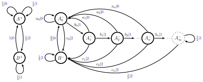
Figure 11: Explosive irreversibility: Despite the forward $\epsilon$-machine $M^{+}$ (left) having just two recurrent causal states, the reverse $\epsilon$-machine $M^{-}$ (right) has a countable infinity of recurrent causal states. Transitions for $M^{-}$ make use of: $a_{n}=2^{n+1}(3z_{n})^{-1}$, $b_{n}=1-(a_{n}+c_{n})$, $c_{n}=3^{n}(2z_{n})^{-1}$, and $z_{n}=2^{n}+3^{n}$. The dashed state labeled $A^{-}_{\infty}$ is an elusive causal state [4]; it is infinitely preceded, but neither reachable (from the omitted start state) nor recurrent. See App. B.

Let us again study the distribution of symbols succeeding histories. Since the process is not Markovian, we cannot expect to obtain the causal states by examining finite-length histories. And so, we must focus attention on semi-infinite histories and their suffixes.

The presence of synchronizing words [43] makes the analysis a bit easier. In this example, $w=0$ and $w=2$ are minimal synchronizing words and, so, after observing one of these words, the state of the $\epsilon$-machine is known with certainty. $\epsilon$-Machine unifilarity then guarantees that on each next symbol we will still know the state of the machine. This allows us to read the distribution of $X_{0}$ directly off the forward $\epsilon$-machine’s outgoing edges.

Thus, any history ending in symbol $0$ will be followed by symbols $0$, $1$, or $2$ with probability $1/3$ each. The equivalence class of histories containing $X_{:0}=\ldots 0$ will be denoted forward causal state $A^{+}$. Looking at the machine, we see that the distribution of next symbols remains unchanged whenever we see a $1$ from state $A^{+}$. So, any history ending in a $0$ followed by an arbitrary, but finite number of $1$s also belongs to equivalence class $A^{+}$. Similarly, any history ending with $2$ will be followed by symbols $1$ or $0$ with probability $1/2$ each. The equivalence class of histories ending in $2$ will be denoted forward causal state $B^{+}$ and, from the machine, we can also see that $B^{+}$ includes any history ending with a $2$ followed by an arbitrary, but finite number of $1$s. A history consisting entirely of the symbol $1$ is best understood by taking the limit of finite histories which also consist entirely of $1$s. When one does this, the history will be followed by symbols $0$ or $1$ with probability $1/2$ each. Concretely, for $X_{0}=(0,1,2)$ and $k\geq 0$, the conditional distributions for every valid history are:

$$\mathbb{P}(X_{0}|X_{:0}=\ldots 01^{k}) =(1/3,1/3,1/3),$$

$$\mathbb{P}(X_{0}|X_{:0}=\ldots 21^{k}) =(1/2,1/2,0),~{}\text{and}$$

$$\mathbb{P}(X_{0}|X_{:0}=1^{\infty}) =(1/2,1/2,0).$$

And, from this, we see that ${\bm{\mathcal{S}}}^{+}=X_{:0}/\sim^{+}$ consists of:

$$A^{+} =\{\ldots 01^{k}\}~{}\text{and}$$

$$B^{+} =\{\ldots 21^{k},1^{\infty}\}.$$

The distribution of symbols preceding futures is more complicated. First, we consider futures beginning with $1^{k}2$, $k\geq 0$. These futures cannot be preceded by symbol $2$. The probability of observing a $0$ or another $1$ preceding these futures is $2/3$ and $1/3$, respectively. We denote the equivalence class of all futures starting with $1^{k}2$ as reverse causal state $B^{-}$. Now, consider all words starting with $1^{k}0$, an arbitrary number of $1$s followed by $0$. A short calculation shows that such words can be preceded by a $0$, $1$, or $2$ with the probability depending explicitly on the number of $1$s at the beginning of the future. Thus, there is one reverse causal state for every $k$, and we denote these states as $A^{-}_{k}$. As before, the future consisting entirely of $1$s is most easily understood by taking limits; one finds that it is not possible to precede the future with a $0$ and that $1$ and $2$ precede the future with probability $1/2$ each. This limiting distribution coincides with $\lim_{k\to\infty}A^{-}_{k}$ and, so, we label its equivalence class $A^{-}_{\infty}$. Formally, for $X_{-1}=(0,1,2)$ and $k\geq 0$, the conditional distributions for every valid future are:

$$\mathbb{P}(X_{-1}|X_{0:}=1^{k}2\ldots) =(2/3,1/3,0),$$

$$\mathbb{P}(X_{-1}|X_{0:}=1^{k}0\ldots) =\textstyle\frac{\left(2^{k+2},\,2^{k+1}+3^{k+1},\,3^{k+1}\right)}{6(2^{k}+3^{k})},~{}\text{and}$$

$$\mathbb{P}(X_{-1}|X_{0:}=1^{\infty}) =(0,1/2,1/2).$$

From this, we see that ${\bm{\mathcal{S}}}^{-}=X_{0:}/\sim^{-}$ consists of:

$$A^{-}_{0} =\{0\ldots\},$$

$$A^{-}_{1} =\{10\ldots\},$$

$$A^{-}_{2} =\{110\ldots\},$$

$$\hskip 5.78172pt\vdots$$

$$A^{-}_{k} =\{1^{k}0\ldots\},$$

$$\hskip 5.78172pt\vdots$$

$$A^{-}_{\infty} =\{1^{\infty}\}$$

$$B^{-} =\{1^{k}2\ldots\}.$$

Again, we leave it to the reader to verify that, for this particular example, a partition of futures into equivalence classes with respect to the preceding symbol will not change when considering longer strings of preceding symbols.

The reverse causal states can also be obtained by applying the forward causal-state equivalence relation on the time-reversed HMM of the forward $\epsilon$-machine. That is, $(X_{0:}/\sim^{-})\cong(\widetilde{X}_{:0}/\sim^{+})$. For example, reverse causal state $A^{-}_{1}$ contains every future beginning with $10$. Alternatively, we can associate $A^{-}_{1}$ with “histories” ($\widetilde{X}_{:0}$) that end $01$. Since the support is reversible, this allows for a direct comparison to the forward causal-state partition, and so $A^{-}_{1}$ is a subset of forward causal state $A^{+}$. We summarize the relationship  between the partitions as follows:

$$A^{+} \cong A^{-}_{0}\cup A^{-}_{1}\cup\cdots\cup A^{-}_{k}\cup\cdots,$$

$$B^{+} \cong B^{-}\cup A^{-}_{\infty}~{}.$$

Recall, $M^{+}_{\emptyset}$ and $M^{-}_{\emptyset}$ denote the forward and reverse DFAs whose structure is defined by the forward and reverse $\epsilon$-machines without probabilities. In this example, $M^{+}_{\emptyset}\neq M^{-}_{\emptyset}$ since they disagree on the number of states. However, $M^{-}_{\emptyset}$ is not minimal and would be equal to $M^{+}_{\emptyset}$, if it were minimized. This means that the support of the process is reversible: $D^{+}=D^{-}$. Thus, this example also demonstrates probability-driven irreversibility, but differs from the example in Sec.VI.2.2, which had $M^{+}_{\emptyset}=M^{-}_{\emptyset}$.

This example demonstrated that the $\epsilon$-machines of irreversible processes can be finite in one direction and infinite in the other. The process has $C_{\mu}^{+}\approx 0.971$ and $C_{\mu}^{-}\approx 1.589$ and, so once again, we see that it takes more memory to generate the process from right-to-left than from left-to-right.

VI.3 Survey of Irreversibility

Reference [3] classified the space of hidden Markov models in terms of unifilarity, synchronization, and minimality. Figure 12 reproduces the essential components of the hierarchy presented there, extending it several ways .

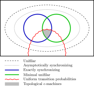
Figure 12: Structural classification of hidden Markov models: Presentations within the green ellipse correspond to the recurrent $\epsilon$-machines. The shaded area is the subset of recurrent $\epsilon$-machines that are exactly synchronizing and, additionally, have uniformly distributed transitions probabilities on the outgoing edges of each state. This subset defines the topological $\epsilon$-machines. Areas in the diagram are not drawn to scale and only show which classes are contained in other classes.

At the outer-most level, outside the dashed ellipse in Fig. 12, we have hidden Markov models that are strictly nonunifilar. So, given the current state and symbol, there is residual uncertainty in the next state: $H[R_{1}|R_{0},{X}_{0}]>0$. Moving inside the dashed ellipse we encounter the strictly unifilar hidden Markov models for which this quantity is exactly zero. Unifilarity is an important property since, among other reasons, it allows one to calculate the process’s entropy rate directly from the presentation.

However, unifilar hidden Markov models can have a type of redundancy such that the state is not justified by the process statistics. Such models have gauge information $\varphi=H[R_{0}|X_{:0},X_{0:}]>0$. And, when we restrict to those with $\varphi=0$, the hidden Markov models become asymptotically synchronizing . This class exists within the dotted ellipse of Fig. 12. One signature of unifilar models with zero gauge information is that the state uncertainty vanishes asymptotically for almost every history in the process language [51].

Within the class of asymptotically synchronizing hidden Markov models, there exists a subset for which the state uncertainty vanishes in finite time for almost every history in the process language [52]. Such hidden Markov models necessarily have at least one synchronizing word. In Fig. 12, this is delineated by the blue ellipse.

Another subset within the class of asymptotically synchronizing hidden Markov models are the minimal unifilar hidden Markov models. Any hidden Markov model with these properties corresponds to an $\epsilon$-machine of a process language [53]. This is represented by the green ellipse in Fig. 12. Generally, the set of $\epsilon$-machines and the set of exactly synchronizing hidden Markov models (blue ellipse) are not the same, and their intersection defines the class of exactly synchronizing $\epsilon$-machines.

Reference [3]’s classification of processes and their presentations provides a natural setting for developing a refined classification based on the irreversibility properties just introduced. As a first step, though, it is perhaps more helpful to develop a quantitative appreciation of how common irreversibility is within the space of hidden Markov models. This is a difficult, if somewhat open-ended challenge, but we can make some progress by examining several subclasses. Systematically surveying presentations is generally difficult due to the probabilistic nature of hidden Markov models and the processes they generate. However, if we restrict ourselves to hidden Markov models with uniformly distributed transition probabilities leaving each state—recall the red, wavy parabola in Fig. 12—then we can systematically enumerate them. Essentially, the task boils down to enumerating a particular class of finite-state automata. Reference [54] provided an exhaustive enumeration of exactly synchronizing $\epsilon$-machines with uniformly distributed transition probabilities leaving each state. It is this class of processes—generated by the topological $\epsilon$-machines—that we survey in order to develop an appreciation of how common irreversibility is within the space of hidden Markov models.

Table 2 summarizes the survey, giving the number $N_{n,k}$ of topological $\epsilon$-machines [54] and the number $C_{n,k}$ of irreversible $\epsilon$-machines over $n$ states and exactly $k$ symbols in the alphabet. (By “exactly $k$ symbols” we emphasize that we excluded from the counts processes with $k=3$ that use only $2$ symbols, for example.) The immediate impression is quite striking: Irreversibility dominates. It comprises over $98\%$ of all topological $\epsilon$-machines and their associated processes. Indeed, the fraction of irreversible $\epsilon$-machines appears to rapidly increase toward unity as the number of states increases. And so, what might have initially appeared to be a counterintuitive property—temporal asymmetry in the statistics of a stationary process—is the overwhelming rule in the space of processes.

$n\backslash k$	$N_{n,2}$	$C_{n,2}$	$N_{n,3}$	$C_{n,3}$	$N_{n,4}$	$C_{n,4}$	$N_{n,5}$	$C_{n,5}$	$N_{n,6}$	$C_{n,6}$
1	1	0	1	0	1	0	1	0	1	0
2	7	0	120	84	1,351	1,200	12,900	12,290	113,827	111,390
3	78	24	15,364	14,561	1,596,682	1,586,736
4	1,388	1,077	3,621,474	3,607,084
5	35,186	33,107
6	1,132,613	1,119,623

Table 2: The number $N_{n,k}$ of topological $\epsilon$-machines [54] and the number $C_{n,k}$ of irreversible $\epsilon$-machines over $n$ states and exactly $k$ symbols in the alphabet.

VII The Bidirectional Machine

The process, as a stationary probability space, is a bulky abstraction, and state-based models, such as hidden Markov models, are often used to provide a much more concise representation. However, the forward and reverse generators of a process are not unique, and this makes it difficult to separate structure in the process from structure in presentations of the process. The entropy rate $h_{\mu}$ and excess entropy ${\bf E}$ are two well known structural properties of a process. We showed, in addition, that crypticity $\chi$, oracular information $\zeta$, and gauge information $\varphi$ are important structural properties of presentations.

The forward and reverse $\epsilon$-machines were introduced as a process’s canonical presentations and, in doing so, the statistical complexities $C_{\mu}^{+}$ and $C_{\mu}^{-}$ became process properties that, in addition, were easily accessible through these privileged presentations. The $\epsilon$-machines were ideal in a number of ways, for example and importantly, they provided a direct calculation of a process’s entropy rate. The excess entropy, however, remained inaccessible and, so, a new presentation was required.

The bidirectional machine, introduced in Refs. [20, 21], is a generator that unites the forward and reverse $\epsilon$-machines, providing an explicit accounting of the relationship between them . In doing so, the excess entropy, a structural property of a process, becomes accessible through a simple calculation and, further, the bidirectional machine contains all information necessary to reconstruct the forward and reverse $\epsilon$-machines. In this section, we define the bidirectional machine and interpret it through an example from the previous section.

VII.1 Definitions

The hidden process lattice of Fig. 7 invites us to consider a dynamic over joint causal states. We define an aggregate state $\mathcal{S}^{\pm}\equiv({\mathcal{S}}^{+},{\mathcal{S}}^{-})$ as the $2$-tuple of the forward and reverse causal states with stationary distribution function:

$$\pi(\alpha\gamma) \equiv\mathbb{P}\left(\mathcal{S}^{\pm}=(\alpha,\gamma)\right)$$

$$=\pi(\alpha,\gamma)$$

$$\equiv\mathbb{P}(\mathcal{S}^{+}=\alpha,\mathcal{S}^{-}=\gamma),$$

for $\alpha\in\mathcal{S}^{+}$ and $\gamma\in\mathcal{S}^{-}$. Counter to typical usage $\pm$ in the joint causal state is interpreted as forward and reverse, rather than or. Note, that we purposefully overload notation and use $\pi$ again, but it will always be clear from context to which generator we refer.

Given the (stationary) distribution $\pi$, if we scan left-to-right, we obtain a forward generator $M^{\pm}$ of the process. If we scan right-to-left, we obtain the process’s reverse generator $M^{\mp}$. These generators are generally distinct. However, we will see that $M^{\mp}$ is equal to the time-reversed HMM of $M^{\pm}$. That is, $M^{\mp}=\widetilde{M}^{\pm}$. For that reason, we take $M^{\pm}$ as the starting point.

Having defined the states, the transition matrices for the forward bidirectional machine $M^{\pm}$ are given by:

$$T_{x}(\alpha\gamma,\beta\delta) \equiv\mathbb{P}\left(X_{0}=x,\mathcal{S}_{1}^{\pm}=(\beta,\delta)\,|\,\mathcal{S}_{0}^{\pm}=(\alpha,\gamma)\right)$$

$$=\begin{cases}\widetilde{T}_{x}(\gamma,\delta)&\text{if }T_{x}(\alpha,\beta)>0,\\ 0&\text{otherwise},\end{cases}$$ (15)

where $\alpha,\beta\in\bm{\mathcal{S}}^{+}$ and $\gamma,\delta\in\bm{\mathcal{S}}^{-}$. The transition probabilities of the forward bidirectional machine mimic the transition probabilities of the time-reversed reverse $\epsilon$-machine ($\widetilde{M}^{-}$), provided the transition is allowed in the forward $\epsilon$-machine ($M^{+}$).

To see how Eq. (VII.1) arises, first we note that:

$$\mathbb{P}\left(X_{0},\mathcal{S}_{1}^{\pm}\,|\,\mathcal{S}_{0}^{\pm}\right)$$

$$=\mathbb{P}\left(X_{0},\mathcal{S}_{1}^{+},\mathcal{S}_{1}^{-}\,|\,\mathcal{S}_{0}^{+},\mathcal{S}_{0}^{-}\right)$$

$$=\mathbb{P}\left(\mathcal{S}_{1}^{+}\,|\,\mathcal{S}_{0}^{+},\mathcal{S}_{0}^{-},X_{0},\mathcal{S}_{1}^{-}\right)\mathbb{P}(X_{0},\mathcal{S}_{1}^{-}\,|\,\mathcal{S}_{0}^{+},\mathcal{S}_{0}^{-})~{}.$$ (16)

Following Eq. (VII.1), we take $\mathcal{S}_{0}^{+}=\alpha$, $\mathcal{S}_{1}^{+}=\beta$, $\mathcal{S}_{0}^{-}=\gamma$, $\mathcal{S}_{1}^{-}=\delta$, and $X_{0}=x$. Then, the first factor in Eq. (VII.1) is either $0$ or $1$, due to unifilarity of the forward $\epsilon$-machine, depending on if $\beta$ is the unique causal state that follows $\alpha$ on symbol $x$. The presence of $\mathcal{S}_{0}^{-}=\gamma$ and $\mathcal{S}_{1}^{-}=\delta$ in the conditional does not change this fact, so long as $(\gamma,x,\delta)$ is a valid consecutive combination in the reverse $\epsilon$-machine—and this is implicitly handled by the second factor.

The second factor reduces due to the shielding property of hidden Markov models: the past and future are independent given the present state. Focusing on the reverse $\epsilon$-machine, we express independence formally as:

$$\mathbb{P}(X_{0:}^{\phantom{+}},{\mathcal{S}}^{-}_{1:}|X_{:0}^{\phantom{+}},{\mathcal{S}}^{-}_{:0},{\mathcal{S}}^{-}_{0})=\mathbb{P}(X_{0:}^{\phantom{+}},{\mathcal{S}}^{-}_{1:}|{\mathcal{S}}^{-}_{0})$$

where $(X_{0:}^{\phantom{+}},{\mathcal{S}}^{-}_{1:})$ is everything related to the future and $(X_{:0}^{\phantom{+}},{\mathcal{S}}^{-}_{:0})$ is everything related to the past. Now, we also know that the forward causal states are determined by the past: $H[{\mathcal{S}}^{+}_{0}|X_{:0}^{\phantom{+}}]=0$, and this means that the forward causal state and future are independent given the past causal state :

$$\mathbb{P}(X_{0:}^{\phantom{+}},{\mathcal{S}}^{-}_{1:}|{\mathcal{S}}^{+}_{0},{\mathcal{S}}^{-}_{0})=\mathbb{P}(X_{0:}^{\phantom{+}},{\mathcal{S}}^{-}_{1:}|{\mathcal{S}}^{-}_{0})$$

Restricting to single-step futures, we obtain:

$$\mathbb{P}(X_{0},\mathcal{S}_{1}^{-}\,|\,\mathcal{S}_{0}^{+},\mathcal{S}_{0}^{-})=\mathbb{P}(X_{0},\mathcal{S}_{1}^{-}\,|\,\mathcal{S}_{0}^{-}).$$ (17)

Understanding this in terms of previously defined quantities is subtle precisely due to the shifting notions of forward and reverse time. Intuitively, Fig. 7 shows that we are asking the reverse $\epsilon$-machine to move left-to-right. This direction is opposed to the reverse $\epsilon$-machine’s local notion of forward time. Thus, we expect this movement from left-to-right to relate to the time-reversed transition matrices of the reverse $\epsilon$-machine.

At a lower level, we note that the definition, Eq. (7), of the time-reversed hidden Markov model was stated under the assumption that the original model’s increasing indexes corresponded to a left-to-right movement on the lattice. From the labeling in Fig. 7, the reverse $\epsilon$-machine does not satisfy this assumption, and a proper translation of Eq. (7) is:

$$\widetilde{T}_{x}(\gamma,\delta) \equiv\mathbb{P}(X_{0}=x,\mathcal{S}^{-}_{1}=\delta\,|\,\mathcal{S}^{-}_{0}=\gamma)$$

$$=\frac{\pi(\delta)T_{x}(\delta,\gamma)}{\pi(\gamma)},$$ (18)

which is exactly the quantity in question. The result is that whenever $T_{x}(\alpha,\beta)>0$, then the transition probability of the forward (left-to-right) bidirectional machine is determined by the transition matrices of the time-reversed reverse $\epsilon$-machine ($\widetilde{M}^{-}$).

Figure 13: Left: Portion of the process lattice relevant to the bidirectional machine’s transition matrices. Right: Realizations of the process lattice as it applies to Eqs. (19), (20), (21), (22), and (23).

The reverse bidirectional machine $M^{\mp}$ is analogously defined by the right-to-left dynamic over the joint causal states. This requires that the forward $\epsilon$-machine move right-to-left on the lattice, a direction that is opposed to its local sense of forward time. The result is that we use the time-reversed forward $\epsilon$-machine ($\widetilde{M}^{+}$). Similarly, the reverse $\epsilon$-machine is required to move right-to-left on the lattice. This direction is in agreement with its local sense of forward time and so, we utilize the reverse $\epsilon$-machine ($M^{-}$) as is. For $\alpha,\beta\in\bm{\mathcal{S}}^{+}$ and $\gamma,\delta\in\bm{\mathcal{S}}^{-}$, we have:

$$\widetilde{T}_{x}(\alpha\gamma,\beta\delta) \equiv\mathbb{P}\left(X_{0}=x,\mathcal{S}_{0}^{\pm}=(\beta,\delta)\,|\,\mathcal{S}_{1}^{\pm}=(\alpha,\gamma)\right)$$

$$=\begin{cases}\widetilde{T}_{x}(\alpha,\beta)&\text{if }T_{x}(\gamma,\delta)>0,\\ 0&\text{otherwise}.\end{cases}$$ (19)

The proof proceeds analogously to the forward bidirectional machine and is omitted here. For future reference, Fig. 13 displays $\alpha$, $\beta$, $\gamma$, and $\delta$ on the process lattice, as they are used in the definition of the reverse bidirectional machine. Thus, we have $\mathcal{S}_{0}^{\pm}=(\beta,\delta)$ and $\mathcal{S}_{1}^{\pm}=(\alpha,\gamma)$. Note, these variables are swapped in the definition of the forward bidirectional machine.

The choice of $\widetilde{T}_{x}$ as the notation for the reverse bidirectional machine’s transition matrices suggests that it is related to the time-reversal of the forward bidirectional machine. Indeed, the definition of the forward bidirectional machine already provides the matrices for the right-to-left dynamic. Thus, we see that $M^{\mp}=\widetilde{M}^{\pm}$:

$$\widetilde{T}_{x}(\alpha\gamma,\beta\delta) \equiv\mathbb{P}\left(X_{0}=x,\mathcal{S}_{0}^{\pm}=(\beta,\delta)\,|\,\mathcal{S}_{1}^{\pm}=(\alpha,\gamma)\right)$$

$$=\frac{\pi(\beta,\delta)T_{x}(\beta\delta,\alpha\gamma)}{\pi(\alpha,\gamma)}~{}.$$ (20)

Applying Eq. (VII.1) gives the direct relation to the forward $\epsilon$-machine:

$$\widetilde{T}_{x}(\alpha\gamma,\beta\delta) =\begin{cases}\frac{\displaystyle\pi(\beta,\delta)\rule[-4.0pt]{0.0pt}{0.0pt}}{\displaystyle\pi(\alpha,\gamma)\rule[0.0pt]{0.0pt}{9.0pt}}\widetilde{T}_{x}(\delta,\gamma)&\text{if }T_{x}(\beta,\alpha)>0,\\ 0&\text{otherwise};\end{cases}$$

$$=\begin{cases}\frac{\displaystyle\pi(\beta\,|\,\delta)\rule[-4.0pt]{0.0pt}{0.0pt}}{\displaystyle\pi(\alpha\,|\,\gamma)\rule[0.0pt]{0.0pt}{9.0pt}}T_{x}(\gamma,\delta)&\text{if }\widetilde{T}_{x}(\alpha,\beta)>0,\\ 0&\text{otherwise}.\end{cases}$$ (21)

Comparing Eqs. (19) and (21), we see that whenever $T_{x}(\gamma,\delta)$ and $\widetilde{T}_{x}(\alpha,\beta)$ are simultaneously positive, then we have:

$$\pi(\alpha\,|\,\gamma)\widetilde{T}_{x}(\alpha,\beta)=\pi(\beta\,|\,\delta)T_{x}(\gamma,\delta)~{}.$$ (22)

A complementary relation, obtained by applying Bayes theorem, is:

$$\pi(\gamma\,|\,\alpha){T}_{x}(\beta,\alpha)=\pi(\delta\,|\,\beta)\widetilde{T}_{x}(\delta,\gamma)~{}.$$ (23)

The interpretations of Eqs.(22) and (23) are properly framed using the process lattice, as shown in Fig. 13. We could have also worked with the forward bidirectional machine, expressing its transition matrix as the Bayes inverse of $\widetilde{T}_{x}$ and, then, equating it to Eq. (VII.1). However, this does not yield any new insight.

Generally, these equations represent path equivalence on the process lattice. In the left-hand side of Eq. (22), we begin in $\mathcal{S}_{1}^{-}=\gamma$, transition to $\mathcal{S}_{0}^{-}=\delta$ on symbol ${X}_{0}=x$, and then shift to $\mathcal{S}_{0}^{+}=\beta$. This path is represented in red in the right diagram of Fig. 14. The right-hand side of Eq. (22) says that the red path is equivalent (in probability) to the blue path, which also begins in $\mathcal{S}_{1}^{-}=\gamma$. However, now it shifts to $\mathcal{S}_{1}^{+}=\alpha$ first, and then reverse transitions to $\mathcal{S}_{0}^{+}=\beta$ on symbol ${X}_{0}=x$. Equation (23) provides an analogous result and is summarized in the left diagram of Fig. 14. There, we begin in $\mathcal{S}_{0}^{+}$ and transition to $\mathcal{S}_{1}^{-}$ via two equivalent paths.

               

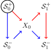
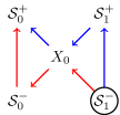
Figure 14: Equations (22) (left) and (23) (right) demonstrate path equivalence. In each, the red and blue paths are equivalent ways of moving around on the process lattice.

The bidirectional machines are so-named because their state space consists of the forward and reverse causal states and their transition dynamic allows one to go in either direction. However, the bidirectional machine is still a one-way generator and this is why there are two variants, $M^{\pm}$ and $M^{\mp}$. These two variants are simply time-reversals of one another, even if the underlying process is irreversible. Having established the proper setting for bidirectional machines, in the next section we analyze several of their properties and the consequences of this symmetry.

VII.2 Bi-Infinite Sequence Partitions

The bidirectional machine $M^{\pm}$ can be understood by analyzing its effect on the past and future. Previously, we saw that the forward causal states ${\mathcal{S}}^{+}$ partitioned the semi-infinite histories $X_{:0}$, while the reverse causal states ${\mathcal{S}}^{-}$ partitioned the semi-infinite futures $X_{0:}$. The bidirectional machine, it turns out, partitions the set of bi-infinite strings $X_{:}\equiv X_{:0}X_{0:}$. This is expressed by the bidirectional equivalence relation [21]:

$$(x_{:0},x_{0:})\sim^{\pm}(x_{:0}^{\prime},x_{0:}^{\prime})\iff\epsilon^{+}(x_{:0}) =\epsilon^{+}(x_{:0}^{\prime})\text{ and }$$

$$\epsilon^{-}(x_{0:}) =\epsilon^{-}(x_{0:}^{\prime})~{}.$$

Thus, the bidirectional causal states ${\bm{\mathcal{S}}}^{\pm}$ are a partition of bi-infinite strings resulting from the application of an equivalence relation: $\bm{\mathcal{S}}^{\pm}=(X_{:0},X_{0:})/\sim^{\pm}$. The mapping $\epsilon^{\pm}(\cdot)$ that takes a bi-infinite string to its bidirectional causal state is defined:

$$\epsilon^{\pm}(x_{:0},x_{0:})$$

$$=\{(x_{:0}^{\prime},x_{0:}^{\prime}):x_{:0}^{\prime}\in\epsilon^{+}(x_{:0})\text{ and }x_{0:}^{\prime}\in\epsilon^{-}(x_{0:})\}~{}.$$

Note, that the same equivalence relation is used for the forward and reverse bidirectional machines. All that differs is the dynamic over the states.

For $M^{\pm}$ and $M^{\mp}$, we use a bi-infinite instance and shift the time origin to the right (for $M^{\pm}$) or to the left (for $M^{\mp}$). The symbol encountered during the shift is the symbol generated.

However, given any bidirectional partition, it does not follow that the dynamic will be unifilar, and this is precisely the case for the bidirectional machines. With $\epsilon$-machines, all histories (or futures) in the equivalence class have exactly the same distribution over futures (or histories). And so, on the next symbol, every history (or future) in the causal state transitioned to the same next causal state. With the bidirectional machine, this is no longer true, and the dynamic over the states is generally nonunifilar.

VII.3 Properties

Each of the process and presentation properties discussed can be considered operators. That is, given a model $M$, we calculate a quantity relative to the model alone, using its local sense of time. This point is worth remembering as we discuss properties of the bidirectional machines. We will continue, however, to frame the various quantities using the bird’s eye view of the process lattice.

The stationary distribution for the forward bidirectional machine is $\mathbb{P}({\mathcal{S}}^{+},{\mathcal{S}}^{-})$ and, as Sec. IV.2 discussed, the reverse bidirectional machine has the same stationary distribution. Using Refs. [20, 21], we can immediately calculate the excess entropy as ${\bf E}=I[{\mathcal{S}}^{+};{\mathcal{S}}^{-}]$. Importantly, this quantity is not calculable given only the forward and reverse $\epsilon$-machines. (Alternate methods to calculate ${\bf E}$ end up being essentially equivalent to invoking the bidirectional machine.)

As mentioned, the bidirectional machine can also be nonunifilar. Since the bidirectional causal states are the joint distribution over the forward and reverse causal states, the bidirectional machine’s oracular information $\zeta(M^{\pm})$ is the crypticity of the reverse $\epsilon$-machine $\chi^{-}$. Additionally, the bidirectional machine’s crypticity $\chi(M^{\pm})$ is the crypticity $\chi^{+}$ of the forward $\epsilon$-machine.

If, instead, we work with the reverse bidirectional machine $M^{\mp}$, all the interpretations are flipped. Then the crypticity $\chi(M^{\mp})$ is equal to the reverse $\epsilon$-machine’s crypticity $\chi^{-}$, and the oracular information $\zeta(M^{\mp})$ is the forward $\epsilon$-machine’s crypticity $\chi^{+}$. Recall that $\epsilon$-machines do not have oracular information, since they are unifilar.

These information quantities are summarized in Fig. 16. There, we see that the reverse bidirectional machine swaps crypticity and oracular information just as a general hidden Markov model [3].

Of the presentation quantifiers, this leaves only the gauge information $\varphi^{\mp}$ to be explained. Recall that the past $X_{:0}$ completely determines the future causal state ${\mathcal{S}}^{+}_{0}$ and that the future $X_{0:}$ completely determines the past causal state ${\mathcal{S}}^{-}$. Then, this gives:

$$\varphi(M^{\pm}) =H[\mathcal{S}^{\pm}|X_{:0},X_{0:}]$$

$$=H[{\mathcal{S}}^{+},{\mathcal{S}}^{-}|X_{:0},X_{0:}]$$

$$=H[{\mathcal{S}}^{+}|X_{:0},X_{0:}]+H[{\mathcal{S}}^{-}|X_{:0},X_{0:},{\mathcal{S}}^{-}]$$

$$\leq H[{\mathcal{S}}^{+}|X_{:0}]+H[{\mathcal{S}}^{-}|X_{0:}]$$

$$=0+0~{}.$$

Thus, the bidirectional machine does have a certain representational efficiency: It has no gauge information. This is implicitly shown in Fig. 16, but more easily seen in Fig. 8. There, we see that the ellipse representing the bidirectional machine’s states (the union of $C_{\mu}^{+}$ and $C_{\mu}^{-}$) only consists of areas within the entropies of the past $H[X_{:0}]$ and future $H[X_{0:}]$. Naturally, one wonders if it is possible to define the bidirectional machine through constraints. To this end, we conjecture that the bidirectional machine is the only generator of the process with zero gauge information that marginalizes into the forward and reverse $\epsilon$-machines and, additionally, has $\chi(M^{\pm})=\chi(M^{+})$ and $\zeta(M^{\pm})=\chi(M^{-})$.

We now turn to the various state entropy quantities that play a role in the bidirectional machine. The state entropy of the forward and reverse $\epsilon$-machines represented the forward and reverse statistical complexities: $C_{\mu}^{+}\equiv H[{\mathcal{S}}^{+}]$ and $C_{\mu}^{-}\equiv H[{\mathcal{S}}^{-}]$. Similarly, we denote the state entropy of the forward and reverse bidirectional machine by $C_{\mu}^{\pm}=H[\mathcal{S}^{\pm}]=H[{\mathcal{S}}^{+},{\mathcal{S}}^{-}]$ and call it the bidirectional statistical complexity. It represents the total amount of information needed to predict or retrodict optimally. The key difference between $C_{\mu}^{\pm}$ and the directed statistical complexities is that with the bidirectional machine, one has a choice in which action, prediction or retrodiction, is taken . We further note that both $C_{\mu}^{+}$ and $C_{\mu}^{-}$ play equivalent roles in $C_{\mu}^{\pm}$, to the extent that ${\bf E}$ is contained in both. Due to this, we can see that:

$$C_{\mu}^{\pm}=C_{\mu}^{+}+C_{\mu}^{-}-{\bf E}~{}.$$ (24)

One can also marginalize the bidirectional machine’s transition matrices to recover the forward and reverse $\epsilon$-machines. For $\alpha,\beta\in\bm{\mathcal{S}}^{+}$ and $\delta,\gamma\in\bm{\mathcal{S}}^{-}$, we marginalize $M^{\pm}$ to get $M^{+}$ as follows:

$$T_{x}(\alpha,\beta) =\mathbb{P}(X_{0}=x,{\mathcal{S}}^{+}_{1}=\beta\,|\,{\mathcal{S}}^{+}_{0}=\alpha)$$

$$=\sum_{\gamma,\delta}\pi(\gamma\,|\,\alpha)\,T_{x}(\alpha\gamma,\beta\delta),$$

where $\pi(\gamma\,|\,\alpha)\equiv\pi(\alpha\gamma)/\pi(\alpha)$ and $T_{x}(\alpha\gamma,\beta\delta)$ is given by Eq. (VII.1). Similarly, we marginalize $M^{\mp}$ to get $M^{-}$:

$$T_{x}(\gamma,\delta) =\mathbb{P}(X_{0}=x,{\mathcal{S}}^{-}_{0}=\delta\,|\,{\mathcal{S}}^{-}_{1}=\gamma)$$

$$=\sum_{\alpha,\beta}\pi(\alpha\,|\,\gamma)\,\widetilde{T}_{x}(\alpha\gamma,\beta\delta),$$

where $\pi(\alpha\,|\,\gamma)\equiv\pi(\alpha\gamma)/\pi(\gamma)$ and $\widetilde{T}_{x}(\alpha\gamma,\beta\delta)$ is given by Eq. (19).

It also happens that knowing the bidirectional causal state is not always helpful. Specifically, we have:

$$H[X_{0}|{\mathcal{S}}^{+}_{0},{\mathcal{S}}^{-}_{0}] =H[X_{0}|{\mathcal{S}}^{-}_{0}]~{}\mathrm{and}$$

$$H[X_{-1}|{\mathcal{S}}^{+}_{0},{\mathcal{S}}^{-}_{0}] =H[X_{-1}|{\mathcal{S}}^{+}_{0}]~{}.$$

In other words, a question about the future is best understood by something which comes from the future (and vice versa for questions about the past). The reason for each of these results can be immediately deduced from Fig. 8.

VII.4 Uses

The bidirectional machine is also useful in a number of ways. We briefly mention several.

First, we note that $M^{\pm}$ and $M^{\mp}$, together, could be interpreted as a transducer. Given a desired direction of time, one can move forward or backward along the process lattice. While the transducer viewpoint holds for any hidden Markov model, only the bidirectional machine allows one to predict or retrodict. To wit, if one constructed a transducer using $M^{+}$ and $\widetilde{M}^{+}$, then one could make predictions, but it would not be possible to retrodict since the forward causal states are not sufficient statistics for the future—they are not suited for retrodiction. This is precisely the advantage of the bidirectional machine, since it tracks both the forward and reverse causal states.

Second, the bidirectional machine allows one to exactly calculate the persistent mutual information $\mathcal{I}_{1}$ [58] over a single-step time interval. Previously available only through empirical estimates, $\mathcal{I}_{1}$ is the amount of information $I[{X}_{:0};{X}_{1:}|{X}_{0}]$ shared between ${X}_{:0}$ and ${X}_{1:}$, ignoring ${X}_{0}$. Note that neither $\epsilon$-machine can give us the appropriate distribution over ${X}_{:0}$ and ${X}_{1:}$, but the bidirectional machine can. And so, it allows one to calculate $\mathcal{I}_{1}$ exactly. Since ${X}_{:0}$ determines $\mathcal{S}_{0}^{+}$ and ${X}_{1:}$ determines $\mathcal{S}_{1}^{-}$, we can write the shared information as $\mathcal{I}_{1}=I[\mathcal{S}_{0}^{+};\mathcal{S}_{1}^{-}]$. The bidirectional machine provides access to the joint distribution $\mathbb{P}({\mathcal{S}}^{+}_{0},{\mathcal{S}}^{-}_{0},{X}_{0},{\mathcal{S}}^{+}_{1},{\mathcal{S}}^{-}_{1})$ and from this, we can calculate $\mathcal{I}_{1}$ in closed-form.

Finally, Refs. [59] and [60] investigated the binding information $b_{\mu}=I[{X}_{0};{X}_{:1}|{X}_{:0}]$ and the residual entropy $r_{\mu}=H[{X}_{0}|{X}_{:0},{X}_{1:}]$. There, they had to be computed essentially by brute force. Fortunately, the bidirectional machine again allows us to compute these exactly and in a manner similar to that for $\mathcal{I}_{1}$. We again replace ${X}_{:0}$ by $\mathcal{S}_{0}^{+}$ and ${X}_{1:}$ by $\mathcal{S}_{1}^{-}$, giving $b_{\mu}=I[{X}_{0};\mathcal{S}_{1}^{-}|\mathcal{S}_{0}^{+}]$ and $r_{\mu}=H[{X}_{0}|\mathcal{S}_{0}^{+},\mathcal{S}_{1}^{-}]$. Here also, the bidirectional machine’s transitions provide the joint distribution $\mathbb{P}(\mathcal{S}_{0}^{+},\mathcal{S}_{0}^{-},{X}_{0},\mathcal{S}_{1}^{+},\mathcal{S}_{1}^{-})$, which can be manipulated appropriately to compute both $b_{\mu}$ and $r_{\mu}$.

In summary, we see that the bidirectional machine gives ready access to closed-form calculations for a wide range of measures in complex processes.

VII.5 Example

We close by returning to the irreversible example of Fig. 9. Its forward $\epsilon$-machine has two causal states while its reverse $\epsilon$-machine has three causal states. When the partitions for each $\epsilon$-machine are logically ANDed together, we obtain the bidirectional machine’s partition over bi-infinite strings.

A compelling visualization of the bidirectional machine’s partition is to superpose the partitions that appeared in Fig. 9. For example, in the forward $\epsilon$-machine, the square corresponding to $X_{-1}X_{0}=21$ was associated with state $A$ (turquoise). In the reverse $\epsilon$-machine, the same square was associated with state $D$ (red-orange). Together, the same square appears in Fig. 15, as both $A$ and $D$.

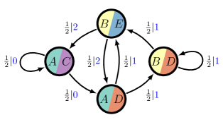
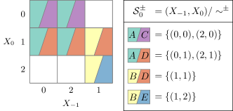
Figure 15: The bidirectional machine $M^{\pm}$ (left) has causal states ${\mathcal{S}}^{\pm}=({\mathcal{S}}^{+},{\mathcal{S}}^{-})$ that partition bi-infinite sequences ${X}_{:}$ of the causally irreversible process of Fig. 9 (right). In this case, it is sufficient to partition sequences using only $(X_{-1},X_{0})$. However, when used as a forward (or reverse) generator, the states of the resulting hidden Markov model $M^{\pm}$ do not correspond to a partition of the pasts (or futures) since the machine is nonunifilar, as is directly checked in the state-transition diagram.

Continuing superposition, we see that there are four bidirectional states and that these four states partition all bi-infinite sequences. In particular, bidirectional state $AD$ includes any sequences ending with a $0$ or $2$ and beginning with a $1$. So, if one learns $C_{\mu}^{\pm}$ bits, then one has the luxury, in this case, of knowing that the next symbol must be a $1$. There is inherent uncertainty in the retrodicting the previous symbol. This is easily verified in the bidirectional machine $M^{\pm}$ (left) of Fig. 15.

Finally, Fig. 16 presents the bidirectional machine’s information diagram sans the past $H[X_{:0}]$ and future $H[X_{0:}]$. The three circles, now drawn to scale, represent the statistical complexities for the forward and reverse $\epsilon$-machines and, also, for the bidirectional machine. Note that the bidirectional machine’s state is simply the combination of the forward and reverse causal states. Calculations give $C_{\mu}^{+}=1$ bit, $C_{\mu}^{-}=3/2$ bit, ${\bf E}=1/2$ bit, $C_{\mu}^{\pm}=2$ bits. This yields $\chi^{+}=\chi(M^{\pm})=\zeta(M^{\mp})=1/2$ bit, $\chi^{-}=\chi(M^{\mp})=\zeta(M^{\pm})=1$ bit and, finally, $\varphi=0$, verifying Eq. (VII.3). The bidirectional machine also gives $\mathcal{I}_{1}=0$, $b_{\mu}=1/2$, and $r_{\mu}=1/2$. Then, according to Ref. [61], the entropy rate is $h_{\mu}=b_{\mu}+r_{\mu}=1$.

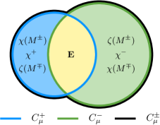
Figure 16: A quantitatively scaled information diagram for the bidirectional machine of Fig. 15. The bidirectional states combine the forward and reverse causal states and are represented by the black, encompassing line. Since the forward (blue) and reverse (green) statistical complexities lay completely within the past and future respectively, the bidirectional machine has no gauge information: $\varphi(M^{\pm})=0$.

VIII Conclusion

The preceding developed a rather thorough survey of reversibility, irreversibility, and time asymmetry—these being understood in the sense of analyzing a process’s statistical and structural properties scanned either in forward or in reverse directions with respect to the direction in which it was given or generated. One result was a stark distinction between Markov chains and hidden Markov models. For one, we explored the ability of hidden Markov models to finitely represent infinite-state Markov chains. This came at a high cost, as we noted: The problem of representational degeneracy appears. We removed this, however, and so were able to present a number of constructive results by using the $\epsilon$-machine as a canonical presentation. Considering that our field of interest is stationary processes, what we found was surprising. First, irreversibility is a dominant property in process space. Second, processes that are finite in one direction can explode into infinite-state processes in the other. And, third, there is a suite of information-theoretic measures, helpfully and constructively captured in various information diagrams, that quantitatively distinguish structural properties of presentations.

The net result is a new appreciation of irreversibility and a new toolkit for analyzing irreversible processes. There are many interesting implications of the long list of technical results. To suggest what these might be and how they will be applied in the near future, we would like to close by returning to the physical motivations called out at the beginning. Specifically, we will comment on the physical meaning of “hidden” processes, the relationship between the diverse irreversibility properties of processes and possible physical instantiations, and, finally, irreversibility in thermodynamic processes.

Why hidden processes? During an interaction between any two systems, only a portion of each system’s internal configuration (or state) is presented to or is available from the other. On the flip side, not every system can take on the full state information of another. In effect, each system views the other as a hidden process. Moreover, in this view measurement is only a special case of interaction. The measurement act typically does not provide all of the observed system’s state. Thus, for measured processes or collections of interacting systems one should view them and analyze them as inherently hidden processes.

Although the analysis largely stayed at the level of probability, statistics, and information, any implementation resides in a physical substrate. This simple observation leads one to immediately ask, How are the statistical and structural properties and classifications of irreversibility related to the organization of a physical substrate? The direct technical answer is that each atom in the process’s information-measure sigma algebra is associated with particular degrees of freedom, structures, and behaviors in a physical implementation. The connection can be made constructively: One of the longest-standing methods to map between continuous-state physical systems and sequences is given by symbolic dynamics [62].

In light of the preceding structural classifications, one now sees that the range of alternate presentations for a process parallels and constrains the range of its possible physical implementations. In this, each different presentation comes with its own distinct set of properties—redundancy, crypticity, oracular information, and the like. In short, then, to study a process’s presentations, to classify them, and to metrize their properties is to study fundamental properties of the associated physical implementations.

Of course, more is required to complete the mapping from a presentation’s intrinsic computation to the required physics. For example, what is the entailed dissipation? This reminds one, naturally, of Landauer’s Principle: A computation’s logical irreversibility is a lower bound on the required amount of energy dissipation in the physical implementation [63]. To the extent that dynamical irreversibility and crypticity control logical irreversibility, then they also put a lower bound on the physical implementation’s rate of energy dissipation. More generally, the development above gives a qualitative lower bound on the richness available and a wide range of applications.

As noted in the Introduction, irreversibility is commonly interpreted as a transient relaxation process. For example, isolated thermodynamic systems move to equilibrium since, according to Boltzmann, there are overwhelmingly more microstates associated with the equilibrium macrostate. This is concisely monitored via the increase in thermodynamic entropy during relaxation from an ordered state. It is enshrined in the Second Law of Thermodynamics. However, as we showed, relaxation is not the only kind of irreversibility that a thermodynamic system can exhibit. There are also irreversibilities, as we analyzed in detail, within nonequilibrium steady states or, equivalently, within general stationary stochastic processes. There, a thermodynamic system is still a process, behaving in time. It is the structure of this temporal behavior that leads to dynamical irreversibility within the set of configuration trajectories—the temporally invariant set consistent with being in a nonequilibrium steady state. The preceding gave a new view of just what these structures are, what irreversibility means in hidden processes, and a general classification scheme for dynamically reversible and irreversible processes.

Concretely, recent explorations of thermodynamic irreversibility and energy dissipation [64, 65, 66] ignore distinctions that are critical for properly identifying statistical irreversibility and intrinsic computation, as laid out here. Thus, the preceding developments provide a detailed analysis that will help these efforts by rectifying and grounding these notions, particularly in terms of the possible physical instantiations of dynamical irreversibility.

Our analysis of how the past and future are contained in the present is addressed to a complex world in which structure and randomness co-exist:

Time present and time past
Are both perhaps present in time future,
And time future contained in time past.

T. S. Eliot, Buirnt Norton, No. 1 of Four Quartets.

In considering general stochastic processes, though, the analysis moves substantially beyond the deterministic world of Laplace’s omniscient Daemon, where initial data is exactly preserved for all times, past and future. Eliot aptly summarizes our exploration of irreversible processes, their pasts and futures, and the role the bidirectional machine plays in capturing the structured present.

Appendix A Markov Order is Time Symmetric

The principal goal here is to review the properties of Markov processes so that we can establish the time-symmetry of the Markov order.

Definition 1.

A process $\mathcal{P}$ is order-$R$ Markov if and only if:

$$\mathbb{P}(X_{0}|X_{:0})=\mathbb{P}(X_{0}|X_{-R:0})~{}.$$ (25)

If $\mathcal{P}$ is order-$R$ Markov, then it is also order-$R{}^{\prime}$ Markov for $R^{\prime}\geq R$. However, it is common to refer to the smallest such $R$ as the Markov order.

Lemma 1.

If a process $\mathcal{P}$ is order-$R$ Markov, then the future depends only on the last $R$ symbols; that is,

$$\mathbb{P}(X_{0:L}|X_{:0})=\mathbb{P}(X_{0:L}|X_{-R:0})~{}.$$ (26)

• By a simple application of the chain rule, we have:

  $$\mathbb{P}(X_{0:L}|X_{:0}) =\prod_{t=0}^{L}\mathbb{P}(X_{t}|X_{:t})$$

  $$=\prod_{t=0}^{L}\mathbb{P}(X_{t}|X_{-R:0},X_{0:t})$$

  $$=\mathbb{P}(X_{0:L}|X_{-R:0})~{}.\qed$$

The result generalizes. The probability of any combination of random variables in the future given the entire past is the same as when given only the last $R$ symbols.

Note that the Markov definition is not time symmetric. This invites another notion of Markovity.

Definition 2.

A process $\mathcal{P}$ is order-$R$ reverse-Markov if and only if:

$$\mathbb{P}(X_{-1}|X_{0:})=\mathbb{P}(X_{-1}|X_{0:R})~{}.$$ (27)

Lemma 2.

If a process $\mathcal{P}$ is order-$R$ reverse-Markov, then the past depends only on the first $R$ symbols:

$$\mathbb{P}(X_{-L:0}|X_{0:})=\mathbb{P}(X_{-L:0}|X_{0:R})~{}.$$ (28)

It happens that the Markov order and reverse Markov orders are always equal.

Theorem 1.

A process $\mathcal{P}$ is order-$R$ Markov if and only if it is order-$R$ reverse-Markov.

• We assume $\mathcal{P}$ is order-$R$ Markov, and then show that $\mathcal{P}$ is order-$R$ reverse-Markov as well. Recall that any joint distribution can be forward factored as:

  $$\mathbb{P}(X_{a:b}) =\prod_{t=a}^{b-1}\mathbb{P}(X_{t}|X_{a:t})~{}.$$

  If the process is Markovian and $(b-a)>R$, then this factoring simplifies to:

  $$\mathbb{P}(X_{a:b}) =\prod_{\mathchoice{\hbox to0.0pt{\hss$\displaystyle{t=a}$\hss}}{\hbox to0.0pt{\hss$\textstyle{t=a}$\hss}}{\hbox to0.0pt{\hss$\scriptstyle{t=a}$\hss}}{\hbox to0.0pt{\hss$\scriptscriptstyle{t=a}$\hss}}}^{\mathchoice{\hbox to0.0pt{\hss$\displaystyle{a+R}$\hss}}{\hbox to0.0pt{\hss$\textstyle{a+R}$\hss}}{\hbox to0.0pt{\hss$\scriptstyle{a+R}$\hss}}{\hbox to0.0pt{\hss$\scriptscriptstyle{a+R}$\hss}}}\mathbb{P}(X_{t}|X_{a:t})\prod_{\mathchoice{\hbox to0.0pt{\hss$\displaystyle{u=a+R+1}$\hss}}{\hbox to0.0pt{\hss$\textstyle{u=a+R+1}$\hss}}{\hbox to0.0pt{\hss$\scriptstyle{u=a+R+1}$\hss}}{\hbox to0.0pt{\hss$\scriptscriptstyle{u=a+R+1}$\hss}}}^{b-1}\mathbb{P}(X_{u}|X_{u-R:u})~{}.$$

  Next, we have:

  $$\mathbb{P}(X_{-1:L}) =\prod_{\mathchoice{\hbox to0.0pt{\hss$\displaystyle{t=-1}$\hss}}{\hbox to0.0pt{\hss$\textstyle{t=-1}$\hss}}{\hbox to0.0pt{\hss$\scriptstyle{t=-1}$\hss}}{\hbox to0.0pt{\hss$\scriptscriptstyle{t=-1}$\hss}}}^{\mathchoice{\hbox to0.0pt{\hss$\displaystyle{R-1}$\hss}}{\hbox to0.0pt{\hss$\textstyle{R-1}$\hss}}{\hbox to0.0pt{\hss$\scriptstyle{R-1}$\hss}}{\hbox to0.0pt{\hss$\scriptscriptstyle{R-1}$\hss}}}\mathbb{P}(X_{t}|X_{-1:t})\prod_{\mathchoice{\hbox to0.0pt{\hss$\displaystyle{u=R}$\hss}}{\hbox to0.0pt{\hss$\textstyle{u=R}$\hss}}{\hbox to0.0pt{\hss$\scriptstyle{u=R}$\hss}}{\hbox to0.0pt{\hss$\scriptscriptstyle{u=R}$\hss}}}^{\mathchoice{\hbox to0.0pt{\hss$\displaystyle{L-1}$\hss}}{\hbox to0.0pt{\hss$\textstyle{L-1}$\hss}}{\hbox to0.0pt{\hss$\scriptstyle{L-1}$\hss}}{\hbox to0.0pt{\hss$\scriptscriptstyle{L-1}$\hss}}}\mathbb{P}(X_{u}|X_{u-R:u})$$

  $$=\mathbb{P}(X_{-1:R})\prod_{\mathchoice{\hbox to0.0pt{\hss$\displaystyle{u=R}$\hss}}{\hbox to0.0pt{\hss$\textstyle{u=R}$\hss}}{\hbox to0.0pt{\hss$\scriptstyle{u=R}$\hss}}{\hbox to0.0pt{\hss$\scriptscriptstyle{u=R}$\hss}}}^{\mathchoice{\hbox to0.0pt{\hss$\displaystyle{L-1}$\hss}}{\hbox to0.0pt{\hss$\textstyle{L-1}$\hss}}{\hbox to0.0pt{\hss$\scriptstyle{L-1}$\hss}}{\hbox to0.0pt{\hss$\scriptscriptstyle{L-1}$\hss}}}\mathbb{P}(X_{u}|X_{u-R:u})$$

  $$=\mathbb{P}(X_{-1}|X_{0:R})\mathbb{P}(X_{0:R})\prod_{\mathchoice{\hbox to0.0pt{\hss$\displaystyle{u=R}$\hss}}{\hbox to0.0pt{\hss$\textstyle{u=R}$\hss}}{\hbox to0.0pt{\hss$\scriptstyle{u=R}$\hss}}{\hbox to0.0pt{\hss$\scriptscriptstyle{u=R}$\hss}}}^{\mathchoice{\hbox to0.0pt{\hss$\displaystyle{L-1}$\hss}}{\hbox to0.0pt{\hss$\textstyle{L-1}$\hss}}{\hbox to0.0pt{\hss$\scriptstyle{L-1}$\hss}}{\hbox to0.0pt{\hss$\scriptscriptstyle{L-1}$\hss}}}\mathbb{P}(X_{u}|X_{u-R:u})$$

  and

  $$\mathbb{P}(X_{0:L}) =\prod_{\mathchoice{\hbox to0.0pt{\hss$\displaystyle{t=0}$\hss}}{\hbox to0.0pt{\hss$\textstyle{t=0}$\hss}}{\hbox to0.0pt{\hss$\scriptstyle{t=0}$\hss}}{\hbox to0.0pt{\hss$\scriptscriptstyle{t=0}$\hss}}}^{\mathchoice{\hbox to0.0pt{\hss$\displaystyle{R}$\hss}}{\hbox to0.0pt{\hss$\textstyle{R}$\hss}}{\hbox to0.0pt{\hss$\scriptstyle{R}$\hss}}{\hbox to0.0pt{\hss$\scriptscriptstyle{R}$\hss}}}\mathbb{P}(X_{t}|X_{0:t})\prod_{\mathchoice{\hbox to0.0pt{\hss$\displaystyle{u=R+1}$\hss}}{\hbox to0.0pt{\hss$\textstyle{u=R+1}$\hss}}{\hbox to0.0pt{\hss$\scriptstyle{u=R+1}$\hss}}{\hbox to0.0pt{\hss$\scriptscriptstyle{u=R+1}$\hss}}}^{\mathchoice{\hbox to0.0pt{\hss$\displaystyle{L-1}$\hss}}{\hbox to0.0pt{\hss$\textstyle{L-1}$\hss}}{\hbox to0.0pt{\hss$\scriptstyle{L-1}$\hss}}{\hbox to0.0pt{\hss$\scriptscriptstyle{L-1}$\hss}}}\mathbb{P}(X_{u}|X_{u-R:u})$$

  $$=\mathbb{P}(X_{0:R+1})\prod_{\mathchoice{\hbox to0.0pt{\hss$\displaystyle{u=R+1}$\hss}}{\hbox to0.0pt{\hss$\textstyle{u=R+1}$\hss}}{\hbox to0.0pt{\hss$\scriptstyle{u=R+1}$\hss}}{\hbox to0.0pt{\hss$\scriptscriptstyle{u=R+1}$\hss}}}^{\mathchoice{\hbox to0.0pt{\hss$\displaystyle{L-1}$\hss}}{\hbox to0.0pt{\hss$\textstyle{L-1}$\hss}}{\hbox to0.0pt{\hss$\scriptstyle{L-1}$\hss}}{\hbox to0.0pt{\hss$\scriptscriptstyle{L-1}$\hss}}}\mathbb{P}(X_{u}|X_{u-R:u})$$

  $$=\mathbb{P}(X_{0:R})\prod_{\mathchoice{\hbox to0.0pt{\hss$\displaystyle{u=R}$\hss}}{\hbox to0.0pt{\hss$\textstyle{u=R}$\hss}}{\hbox to0.0pt{\hss$\scriptstyle{u=R}$\hss}}{\hbox to0.0pt{\hss$\scriptscriptstyle{u=R}$\hss}}}^{\mathchoice{\hbox to0.0pt{\hss$\displaystyle{L-1}$\hss}}{\hbox to0.0pt{\hss$\textstyle{L-1}$\hss}}{\hbox to0.0pt{\hss$\scriptstyle{L-1}$\hss}}{\hbox to0.0pt{\hss$\scriptscriptstyle{L-1}$\hss}}}\mathbb{P}(X_{u}|X_{u-R:u})~{}.$$

  So, finally, we obtain the desired result:

  $$\mathbb{P}(X_{-1}|X_{0:L}) =\frac{\mathbb{P}(X_{-1:L})}{\mathbb{P}(X_{0:L})}$$

  $$=\mathbb{P}(X_{-1}|X_{0:R})~{}.$$

  In the other direction, we use the reverse factoring of a joint distribution:

  $$\mathbb{P}(X_{a:b}) =\prod_{\mathchoice{\hbox to0.0pt{\hss$\displaystyle{t=a}$\hss}}{\hbox to0.0pt{\hss$\textstyle{t=a}$\hss}}{\hbox to0.0pt{\hss$\scriptstyle{t=a}$\hss}}{\hbox to0.0pt{\hss$\scriptscriptstyle{t=a}$\hss}}}^{\mathchoice{\hbox to0.0pt{\hss$\displaystyle{b-1}$\hss}}{\hbox to0.0pt{\hss$\textstyle{b-1}$\hss}}{\hbox to0.0pt{\hss$\scriptstyle{b-1}$\hss}}{\hbox to0.0pt{\hss$\scriptscriptstyle{b-1}$\hss}}}\mathbb{P}(X_{t}|X_{t+1:b})~{}.$$

  Then, we assume the process is reverse-Markov to obtain:

  $$\mathbb{P}(X_{a:b}) =\prod_{\mathchoice{\hbox to0.0pt{\hss$\displaystyle{t=a}$\hss}}{\hbox to0.0pt{\hss$\textstyle{t=a}$\hss}}{\hbox to0.0pt{\hss$\scriptstyle{t=a}$\hss}}{\hbox to0.0pt{\hss$\scriptscriptstyle{t=a}$\hss}}}^{\mathchoice{\hbox to0.0pt{\hss$\displaystyle{b-R-2}$\hss}}{\hbox to0.0pt{\hss$\textstyle{b-R-2}$\hss}}{\hbox to0.0pt{\hss$\scriptstyle{b-R-2}$\hss}}{\hbox to0.0pt{\hss$\scriptscriptstyle{b-R-2}$\hss}}}\mathbb{P}(X_{t}|X_{t+1:t+1+R})\prod_{\mathchoice{\hbox to0.0pt{\hss$\displaystyle{u=b-R-1}$\hss}}{\hbox to0.0pt{\hss$\textstyle{u=b-R-1}$\hss}}{\hbox to0.0pt{\hss$\scriptstyle{u=b-R-1}$\hss}}{\hbox to0.0pt{\hss$\scriptscriptstyle{u=b-R-1}$\hss}}}^{\mathchoice{\hbox to0.0pt{\hss$\displaystyle{b-1}$\hss}}{\hbox to0.0pt{\hss$\textstyle{b-1}$\hss}}{\hbox to0.0pt{\hss$\scriptstyle{b-1}$\hss}}{\hbox to0.0pt{\hss$\scriptscriptstyle{b-1}$\hss}}}\mathbb{P}(X_{t}|X_{t+1:b})~{}.$$

  Similarly, we have:

  $$\mathbb{P}(X_{-L:1}) =\mathbb{P}(X_{0}|X_{-R:0})\mathbb{P}(X_{-R:0})$$

  $$\qquad\times\prod_{\mathchoice{\hbox to0.0pt{\hss$\displaystyle{t=-L}$\hss}}{\hbox to0.0pt{\hss$\textstyle{t=-L}$\hss}}{\hbox to0.0pt{\hss$\scriptstyle{t=-L}$\hss}}{\hbox to0.0pt{\hss$\scriptscriptstyle{t=-L}$\hss}}}^{\mathchoice{\hbox to0.0pt{\hss$\displaystyle{-(R+1)}$\hss}}{\hbox to0.0pt{\hss$\textstyle{-(R+1)}$\hss}}{\hbox to0.0pt{\hss$\scriptstyle{-(R+1)}$\hss}}{\hbox to0.0pt{\hss$\scriptscriptstyle{-(R+1)}$\hss}}}\mathbb{P}(X_{t}|X_{t+1:t+1+R})$$

  and

  $$\mathbb{P}(X_{-L:0}) =\mathbb{P}(X_{-R:0})\prod_{\mathchoice{\hbox to0.0pt{\hss$\displaystyle{t=-L}$\hss}}{\hbox to0.0pt{\hss$\textstyle{t=-L}$\hss}}{\hbox to0.0pt{\hss$\scriptstyle{t=-L}$\hss}}{\hbox to0.0pt{\hss$\scriptscriptstyle{t=-L}$\hss}}}^{\mathchoice{\hbox to0.0pt{\hss$\displaystyle{-(R+1)}$\hss}}{\hbox to0.0pt{\hss$\textstyle{-(R+1)}$\hss}}{\hbox to0.0pt{\hss$\scriptstyle{-(R+1)}$\hss}}{\hbox to0.0pt{\hss$\scriptscriptstyle{-(R+1)}$\hss}}}\mathbb{P}(X_{t}|X_{t+1:t+1+R})~{}.$$

  Then,

  $$\mathbb{P}(X_{0}|X_{-L:0}) =\frac{\mathbb{P}(X_{-L:1})}{\mathbb{P}(X_{-L:0})}$$

  $$=\mathbb{P}(X_{0}|X_{-R:0})~{}.$$

  The results hold for every $L>R$ and in the $L\to\infty$ limit, too. ∎

The two notions of Markovity relate to forward and reverse generators.

Lemma 3.

The forward generator $M^{+}$ is order-$R$ Markov if and only if the reverse generator is order-$R$ reverse-Markov.

• This follows directly from the definition of the reverse process. Assume $M^{+}$ has Markov order $R$. Let $|u|=L-2R$ and $|w|=|v|=R$. Then,

  $$\mathbb{P}(\widetilde{X}_{-1}|\widetilde{X}_{0:L}=wuv) =\mathbb{P}(X_{1}|X_{-L+1:1}=\widetilde{v}\widetilde{u}\widetilde{w})$$

  $$=\mathbb{P}(X_{1}|X_{-R+1:1}=\widetilde{w})$$

  $$=\mathbb{P}(\widetilde{X}_{-1}|\widetilde{X}_{0:R}=w)~{}.\qed$$

With this interpretation, it is a short step to see that the Markov order is reversible.

Corollary 1.

The forward generator is order-$R$ Markov if and only the reverse generator is order-$R$ Markov.

• Apply Thm. 1 and then Lem. 3. ∎

Appendix B The Explosive Example Revisited

In Sec. VI.2.3, we examined a causally irreversible process whose forward $\epsilon$-machine had two causal states, while its reverse $\epsilon$-machine had a countable infinity of causal states. Here, we provide details for calculating this reverse $\epsilon$-machine from the forward $\epsilon$-machine. We give expressions for the excess entropy and statistical complexities. A detailed analysis of the various kinds of causal states—recurrent, transient, and elusive—for the forward and reverse $\epsilon$-machines appears in Fig. 17 and gives some insight into the origins of the reverse $\epsilon$-machine’s infinite number of causal states.

The forward and reverse $\epsilon$-machines are shown in Fig. 17. The entropy rate, since it is reversible [69], is easier to calculate from $M^{+}$. This is given directly:

$$h_{\mu} =H[X_{0}|{\mathcal{S}}^{+}_{0}]$$

$$=\frac{3}{5}\log_{2}3+\frac{2}{5}$$ (29)

$$\approx 1.350\ 955\ 500\ 432~{}.$$

The forward statistical complexity is:

$$C_{\mu}^{+} =\frac{3}{5}\log_{2}\frac{5}{3}+\frac{2}{5}\log_{2}\frac{5}{2}$$ (30)

$$\approx 0.970\ 950\ 594\ 455~{}.$$

For $n\geq 0$, the mixed-state operator [21] acting on $\widetilde{M}^{\pm}$ gives:

$$\mathbb{P}({\mathcal{S}}^{+}_{0}|{\mathcal{S}}^{-}_{0}=A_{n-1}^{-}) =\biggl{(}\frac{3\cdot 2^{n}}{3\cdot 2^{k}+2\cdot 3^{n}},\frac{2\cdot 3^{n}}{3\cdot 2^{n}+2\cdot 3^{n}}\biggr{)}$$

and

$$\mathbb{P}({\mathcal{S}}^{+}_{0}|{\mathcal{S}}^{-}_{0}=B^{-}) =(1,0)~{}.$$

As it turns out, these distributions are also the mixed states for the transient causal states of $M^{+}$ in the basis of its recurrent states. That is:

$$\mathbb{P}({\mathcal{S}}^{+}_{0}|{\mathcal{S}}^{+}_{0}=D_{n}^{+}) =\mathbb{P}({\mathcal{S}}^{+}_{0}|{\mathcal{S}}^{-}_{0}=A_{n-1}^{-})~{}.$$

To determine $\pi({\mathcal{S}}^{-})$ we solve the following simultaneous equations:

$$\pi(B^{-}) =\frac{1}{3}\pi(B^{-})+\sum_{n=0}^{\infty}c_{n}\pi(A_{n}^{-})$$

$$\pi(A_{0}^{-}) =\frac{2}{3}\pi(B^{-})+\sum_{n=0}^{\infty}a_{n}\pi(A_{n}^{-})$$

$$\pi(A_{n}^{-}) =b_{n-1}\pi(A_{n-1}^{-})\qquad n>0~{}.$$

Beginning with the third, we have:

$$\pi(A_{n}^{-}) =b_{n-1}\pi(A_{n-1}^{-})$$

$$=\left(\,\prod_{n=0}^{n-1}b_{n}\right)\pi(A_{0}^{-})$$

$$=\left(\frac{1+\frac{2}{3}^{n}}{2^{n+1}}\right)\pi(A_{0}^{-})~{},$$

for $n>0$. Then, solving for $\pi(B^{-})$, gives:

$$\pi(B^{-}) =\frac{3}{2}\sum_{n=0}^{\infty}c_{n}\pi(A_{n}^{-})~{}.$$

So,

$$\pi(B^{-}) =\frac{3}{4}\pi(A_{0}^{-})~{}.$$

The normalization constraint becomes:

$$1 =\pi(B^{-})+\sum_{n=0}^{\infty}\pi(A_{n}^{-})$$

$$=\frac{3}{4}\pi(A_{0}^{-})+\frac{7}{4}\pi(A_{0}^{-})~{}.$$

Thus,

$$\pi(A_{n}^{-}) =\frac{1+\left(\frac{2}{3}\right)^{n}}{5\cdot 2^{n}}$$

$$\pi(B^{-}) =\frac{3}{10}~{}.$$

Collecting these together, we find:

$$C_{\mu}^{-} =\frac{3}{10}\log_{2}\frac{10}{3}-\sum_{n=0}^{\infty}\left(\frac{1+\left(\frac{2}{3}\right)^{n}}{5\cdot 2^{n}}\right)\log_{2}\left(\frac{1+\left(\frac{2}{3}\right)^{n}}{5\cdot 2^{n}}\right)$$

$$\approx 1.588\ 621\ 621\ 714~{}.$$

Finally,

$${\bf E} =C_{\mu}^{+}-H[{\mathcal{S}}^{+}|{\mathcal{S}}^{-}]$$

$$=C_{\mu}^{+}-\sum_{n=0}^{\infty}\left(\frac{1+\left(\frac{2}{3}\right)^{n}}{5\cdot 2^{n}}\right)H\left(\frac{3\cdot 2^{n}}{3\cdot 2^{k}+2\cdot 3^{n}}\right)$$

$$\approx 0.304\ 159\ 734\ 344~{},$$

where $H(\cdot)$ is the binary entropy function.

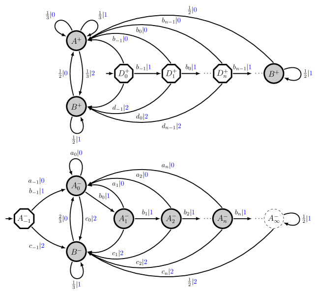
Figure 17: The forward $\epsilon$-machine $M^{+}$ (top) has only two recurrent (shaded) causal states $A^{+}$ and $B^{+}$. The reverse $\epsilon$-machine $M^{-}$ (bottom) has an infinite number of recurrent causal states. Transition labels in both machines make use of: $a_{n}=2^{n+1}(3z_{n})^{-1}$, $b_{n}=1-(a_{n}+c_{n})$, $c_{n}=3^{n}(2z_{n})^{-1}$, $d_{n}=1-2b_{n}$, and $z_{n}=2^{n}+3^{n}$. The dashed state labeled $A_{\infty}^{-}$ is an elusive causal state [4]: It is infinitely preceded, but neither reachable nor recurrent. The hexagon-shaped states are strictly transient states and only induced by finite-length histories. Note, the limit of the $D_{n}^{+}$ states is $D_{\infty}^{+}=B^{+}$ and it was drawn separately only to demonstrate the trend.

References

- [1] P. S. de Laplace. A Philosophical Essay on Probabilities. Dover, New York, 1952.
- [2] Note that thermodynamics does speak of reversible macroscopic processes. Consider, for example, a common thermodynamic process: the isobaric expansion of a gas from macrostate with volume , temperature , and pressure to macrostate with volume and temperature at pressure . This process is called reversible, if there exists a way of manipulating the gas back to macrostate , once it is found in macrostate , such as by cooling it. This notion of thermodynamic reversibility, however, differs from our notion of reversibility which focuses on the ability to reconstruct a history from observations.
- [3] J. P. Crutchfield, C. J. Ellison, J. R. Mahoney, and R. G. James. Synchronization and control in intrinsic and designed computation: An information-theoretic analysis of competing models of stochastic computation. CHAOS, 20(3):037105, 2010.
- [4] D. R. Upper. Theory and Algorithms for Hidden Markov Models and Generalized Hidden Markov Models. PhD thesis, University of California, Berkeley, 1997. Published by University Microfilms Intl, Ann Arbor, Michigan.
- [5] This is equivalent to index notation in the Python programming language.
- [6] This is yet another reminder that probability alone cannot determine causality [67].
- [7] D. A. Levin, Y. Peres, and E. L. Wilmer. Markov Chains and Mixing Times. American Mathematical Society, 1st edition, 2008.
- [8] J. P. Crutchfield. The calculi of emergence: Computation, dynamics, and induction. Physica D, 75:11–54, 1994.
- [9] L. P. Kelly. Reversibility and Stochastic Networks. Wiley, Chichester, 1979.
- [10] Y. Ephraim and N. Merhav. Hidden markov processes. IEEE Trans. Info. Theory, 48:1518–1569, 2002.
- [11] L. E. Baum and T. Petrie. Statistical inference for probabilistic functions of finte state markov chains. Annals of Mathematical Statistics, 37:1554–1563, 1966.
- [12] I. MacDonald and W. Zucchini. Hidden Markov and Other Discrete-valued Time Series. Chapman & Hill, London, 1997.
- [13] In Ref. [12], it was shown that Poisson-valued, state-emitting hidden Markov models are reversible if their internal Markov chains are reversible. This result does not hold with edge-emitting hidden Markov models, as demonstrated by example.
- [14] A similar statement can be made of Markov chains since the process generated by a Markov chain is reversible if and only the Markov chain is in detailed balance.
- [15] D. Blackwell and L. Koopmans. On the identifiability problem for functions of Markov chains. Ann. Math. Statist., 28:1011, 1957.
- [16] H. Ito, S.-I. Amari, and K. Kobayashi. Identifiability of hidden Markov information sources and their minimum degrees of freedom. IEEE Info. Th., 38:324, 1992.
- [17] V. Balasubramanian. Equivalence and reduction of hidden markov models. A.I. Tech Report 1370, Massachusetts Institute of Technology, January 1993.
- [18] B. Weiss. Subshifts of finite type and sofic systems. Monastsh. Math., 77:462, 1973.
- [19] T. M. Cover and J. A. Thomas. Elements of Information Theory. Wiley-Interscience, New York, second edition, 2006.
- [20] J. P. Crutchfield, C. J. Ellison, and J. R. Mahoney. Time’s barbed arrow: Irreversibility, crypticity, and stored information. Phys. Rev. Lett., 103(9):094101, 2009.
- [21] C. J. Ellison, J. R. Mahoney, and J. P. Crutchfield. Prediction, retrodiction, and the amount of information stored in the present. J. Stat. Phys., 136(6):1005–1034, 2009.
- [22] R. W. Yeung. A new outlook on Shannon’s information measures. IEEE Trans. Info. Th., 37(3):466–474, 1991.
- [23] T. Kawabata and R. W. Yeung. The structure of the I-measure of a markov chain. IEEE Trans. Info. Th., 38(3):1146–1149, 1992.
- [24] C. E. Shannon and W. Weaver. The Mathematical Theory of Communication. University of Illinois Press, Champaign-Urbana, 1962.
- [25] Keep in mind that, unless otherwise stated, these figures are not drawn to scale. For example, the entropy of the past is infinite. Since the drawings are not scale, we use the term circle liberally. Despite this, the important relationships of the variables are preserved.
- [26] A. del Junco and M. Rahe. Finitary codings and weak bernoulli partitions. Proc. AMS, 75:259, 1979.
- [27] J. P. Crutchfield and N. H. Packard. Symbolic dynamics of noisy chaos. Physica, 7D:201 – 223, 1983.
- [28] P. Grassberger. Toward a quantitative theory of self-generated complexity. Intl. J. Theo. Phys., 25:907, 1986.
- [29] W. Bialek, I. Nemenman, and N. Tishby. Predictability, complexity, and learning. Neural Computation, 13:2409–2463, 2001.
- [30] J. P. Crutchfield and D. P. Feldman. Regularities unseen, randomness observed: Levels of entropy convergence. Chaos: An Interdisciplinary Journal of Nonlinear Science, 13(1):25–54, 2003.
- [31] J. R. Mahoney, C. J. Ellison, and J. P. Crutchfield. Information accessibility and cryptic processes. J. Phys. A: Math. Theo., 42:362002, 2009.
- [32] J. P. Crutchfield and K. Young. Inferring statistical complexity. Phys. Rev. Let., 63:105–108, 1989.
- [33] C. R. Shalizi and J. P. Crutchfield. Computational mechanics: Pattern and prediction, structure and simplicity. J. Stat. Phys., 104:817–879, 2001.
- [34] E. M. Coven and M. E. Paul. Sofic systems. Israel. J. Math., 20:165, 1975.
- [35] W. Löhr and N. Ay. On the generative nature of prediction. Advances in Complex Systems, 12(2):169–194, 2009.
- [36] The entropy of the distribution of distributions over states is precisely the -machine’s statistical complexity .
- [37] J. E. Hopcroft and J. D. Ullman. Introduction to Automata Theory, Languages, and Computation. Addison-Wesley, Reading, 1979.
- [38] D. Angluin. Inference of reversible languages. J. ACM, 29:741–765, July 1982.
- [39] J.-E. Pin. On reversible automata. In LATIN ’92, volume 583 of Lecture Notes in Computer Science, pages 401–416. Springer Berlin / Heidelberg, 1992.
- [40] S. Lombardy. On the construction of reversible automata for reversible languages. In Automata, Languages and Programming, volume 2380 of Lecture Notes in Computer Science, pages 787–787. Springer Berlin / Heidelberg, 2002.
- [41] J. Sempere. Learning reversible languages with terminal distinguishability. In Grammatical Inference: Algorithms and Applications, volume 4201 of Lecture Notes in Computer Science, pages 354–355. Springer Berlin / Heidelberg, 2006.
- [42] P. García, M. Vázquez de Parga, A. Cano, and D. López. On locally reversible languages. Theoretical Computer Science, 410(47-49):4961–4974, 2009.
- [43] R. G. James, J. R. Mahoney, C. J. Ellison, and J. P. Crutchfield. submitted, 2010. arxiv.org:1010.5545 [nlin.CD].
- [44] In this work and also in Ref. [21], two equivalence relations were defined. The forward equivalence relation partitioned , while the reverse equivalence relation partitioned . However, these relations are formally the same in that they both partition a generator’s local time histories. To see this, recall that is isomorphic to .
- [45] In this example, it is sufficient to consider length- futures, but we use length- futures in order to demonstrate the general technique. That is, the columns of the matrix representing the conditional distribution must be marginalized in order to obtain the transition probabilities of the -machine.
- [46] It is much easier to see that the forward and reverse -machines are irreversible if matrix is compared to matrix , instead of to matrix . Matrices and are in the local time perspective and, thus, their forms are directly comparable. Matrix , in contrast, is in the global (lattice) perspective of Fig. 7 and requires index manipulation to see that the resultant dynamics are irreversible.
- [47] Note that since the forward -machine is finite, the process does have a finite reverse generator—namely, the time-reversed forward -machine. However, the minimality of the -machine, within the class of unifilar HMMs, ensures that this presentation can be smaller than the reverse -machine only if it is also nonunifilar.
- [48] This relationship is a comparison between the forward and reverse causal states only. To each forward causal state, there is a 1-1 correspondence between its histories and the union of futures from reverse causal states. Note that this relationship says little about how the partitions are correlated in time. For that, one must consider . See App. B.
- [49] In Fig. 12, we stress that some atoms may have zero measure. For example, every -machine with uniformly distributed transition probabilities is exactly synchronizing. Thus, the atom representing hidden Markov models with uniformly distributed transition probabilities that are simultaneously minimal unifilar and not exactly synchronizing is empty.
- [50] Reference [3] called this class weakly asymptotically synchronizing, but it turns out to be equivalent to (strongly) asymptotically synchronizing [68].
- [51] N. Travers and J. P. Crutchfield. Asymptotically synchronizing to finitary sources. 2010. SFI Working Paper 10-11-029; arxiv.org:1011.1581 [nlin.CD].
- [52] N. Travers and J. P. Crutchfield. Exactly synchronizing to finitary sources. 2010. SFI Working Paper 10-11-031; arxiv.org:1008.4182 [nlin.CD].
- [53] N. Travers and J. P. Crutchfield. Equivalence of history and generator epsilon-machines. 2010. SFI Working Paper 10-12-XXX; arxiv.org:1012.XXXX [XXXX].
- [54] B. D. Johnson, J. P. Crutchfield, C. J. Ellison, and C. S. McTague. submitted, 2010. arxiv.org:1011.0036 [cs.FL].
- [55] Given the forward -machine of a process, one can construct its reverse -machine using the technique described in Ref. [21]. From this construction, we learn how the forward and reverse causal states are related. However, if one is given only the reverse -machine, then this important information is lost and must be deduced again. The bidirectional machine is a presentation of the process that preserves this information.
- [56] Let , , , and be random variables such that maps deterministically onto . Further, suppose that and are independent given . Then it follows that and are also independent given .
- [57] One must choose only one action: prediction or retrodiction. The forward bidirectional machine allows one to make a prediction, while the reverse bidirectional machine allows one to make a retrodiction. Making a simultaneous prediction and retrodiction with each machine does not yield the correct joint probabilities over predicted and retrodicted symbols.
- [58] R. C. Ball, M. Diakonova, and R. S. MacKay. Quantifying Emergence in Terms of Persistent Mutual Information. Advances in Complex Systems, 13(3):327–338, 2010.
- [59] S. A. Abdallah and M. D. Plumbley. A Measure of Statistical Complexity Based on Predictive Information. (unpublished), 2010.
- [60] S. A. Abdallah and M. D. Plumbley. Predictive Information, Multi-Information, and Binding Information. Technical Report C4DM-TR10-10, Centre for Digital Music, Queen Mary University of London, 2010.
- [61] R. G. James, C. J. Ellison, and J. P. Crutchfield. Anatomy of a bit: Information in a time series observation. page submitted, 2010. Santa Fe Institute Working Paper 11-05-XXX; arxiv.org:1105.2988 [math.IT].
- [62] D. Lind and B. Marcus. An Introduction to Symbolic Dynamics and Coding. Cambridge University Press, New York, 1995.
- [63] R. Landauer. Dissipation and noise immunity in computation, measurement, and communication. J. Stat. Phys., 54(5/6):1509–1517, 1989.
- [64] C. Jarzynski. Nonequilibrium equality for free energy differences. Phys. Rev. Lett., 78(14):2690–2693, 1997.
- [65] G. E. Crooks. Nonequilibrium measurements of free energy differences for microscopically reversible markovian systems. J. Stat. Phys., 90(5/6):1481–1487, 1998.
- [66] S. Toyabe, T. Sagawa, M. Ueda, E. Muneyuki, and M. Sano. Experimental demonstration of information-to-energy conversion and validation of the generalized jarzynski equality. Nature Physics, 6:988–992, 2010.
- [67] J. Pearl. Causality: Models, Reasoning and Inference. Cambridge University Press, 2nd edition, 2009.
- [68] N. Travers. 2011. Personal communication.
- [69] J. P. Crutchfield and C. R. Shalizi. Thermodynamic depth of causal states: Objective complexity via minimal representations. Phys. Rev. E, 59(1):275–283, 1999.