Generalized Density Matrix Revisited: Microscopic Approach to Collective Dynamics in Soft Spherical Nuclei

Abstract

The generalized density matrix (GDM) method is used to calculate microscopically the parameters of the collective Hamiltonian. Higher order anharmonicities are obtained consistently with the lowest order results, the mean field [Hartree-Fock-Bogoliubov (HFB) equation] and the harmonic potential [quasiparticle random phase approximation (QRPA)]. The method is applied to soft spherical nuclei, where the anharmonicities are essential for restoring the stability of the system, as the harmonic potential becomes small or negative. The approach is tested in three models of increasing complexity: the Lipkin model, model with factorizable forces, and the quadrupole plus pairing model.

I Introduction

A long-standing question of microscopic description of nuclear collective motion belongs to the class of problems which are left behind by the advancing army that currently is mostly interested in new frontiers, in our case, in drip line physics. Meanwhile, we still lack a systematic theory based on first principles and inter-nucleon interactions that would allow us to fully understand numerous collective phenomena in the low-energy region of medium and heavy nuclei and satisfactorily describe the data. In relatively light nuclei, the shell model (what is nowadays called configuration interaction) with effective nucleon-nucleon forces usually works well although even here the abundant numerical results sometimes require some kind of model interpretation. In heavier nuclei, the necessary orbital space is too large for direct numerical diagonalization.

Phenomenological models frequently work well, first of all the geometric Bohr Hamiltonian Bohr ; Bohr_Hamil and the interacting boson model (IBM) IBM . However, the relation between their parameters and the underlying microscopic structure remains uncertain. Moreover, some assumptions of such models turn out to be unreliable. For example, the identification in the IBM of the prescribed boson number with the number of valence fermionic pairs breaks down in the attempt to explain very long “quasivibrational” bands extended, without considerable changes in spacing, up to spin values much greater than the finite boson number would allow, see for example the ground state band in ¹¹⁰Cd close to the equidistant ladder up to $J^{\pi}=28^{+}$.

The microscopic theory is relatively successful in well deformed nuclei. Various mean-field methods, including the modern energy density functional approach DFT1 ; DFT2 with pairing, indicate regions of nuclei with clearly pronounced deformed energy minima. With the microscopic definition of shape, one can calculate the moment of inertia by the cranking model and the generator coordinate method, construct rotational bands built on different intrinsic configurations and explain back-bending and similar phenomena Back_Bending .

In our opinion, the status of microscopic theory is still underdeveloped with respect to spherical nuclei, especially in the case of the presence of a low-lying collective mode. The standard way of defining such modes is based on the quasiparticle random phase approximation (QRPA). This is essentially the harmonic approximation that determines the frequency and two-quasiparticle structure of the collective phonons. If the multipole coupling is strong, the collective mode has a large amplitude, the frequency falls down, and the QRPA reveals the instability. In reality, this is not necessarily a point of phase transition. Rather, this is the region of strong anharmonicities outside of the reach of the QRPA. Phenomenologically, this can be described by a special choice of potential and rotational parameters in the Bohr Hamiltonian which are close to the ${\cal O}(6)$ limit of the IBM with a gamma-unstable potential. Currently we do not have a reliable microscopic approach to quantify collective behavior of this type. Another practically important question related to anharmonicities is the mode-mode coupling. The coexistence and interaction of soft quadrupole and octupole modes are relevant, for example, to the search of mechanisms for many-body enhancement of the nuclear Schiff moment and the atomic electric dipole moment Mul_Mode .

Instead of the direct diagonalization of the primary nucleon Hamiltonian, it seems reasonable to work out a procedure for the microscopic derivation of the effective collective Hamiltonian. Typical collective states can usually be identified by their quantum numbers, low energies and large transition probabilities. Being interconnected by large matrix elements of corresponding collective operators they form a collective subspace of the total Hilbert space of the system. In the case of a soft multipole mode, it is often possible to label the empirical levels by the phonon quantum numbers, even if their energies and transition rates noticeably differ from the predictions of the harmonic approximation. This difference results from anharmonic effects which still keep the geometric nature of the mode. Therefore our approach will be to develop the road to a consistent mapping of the underlying nucleonic dynamics onto that inside the collective subspace.

The idea of this approach goes back to the boson expansion technique suggested long ago first_anh ; a detailed review of work in this direction can be found in rmp_boson . The formalism of the generalized density matrix (GDM) reformulating earlier work GDM_Klein by Kerman and Klein seems to be the most appropriate for our goal BZ1 ; BZ2 ; BZ3 ; Zele_ptps . This formalism was applied to collective rotation BZ1 ; BZ3 ; BZ4 ; Zele5 and large amplitude collective motion LA1 ; LA2 ; LA3 ; LA4 generalizing the time-dependent mean-field method Negele . Here we apply the GDM approach to collective vibrations in soft spherical nuclei.

The generalized density matrix $R_{12}=a^{\dagger}_{2}a_{1}$ is the set of operators defined originally in the entire Hilbert space [1 and 2 here represent a complete set of single-particle (s.p.) quantum numbers]. The microscopic Hamiltonian provides exact operator equations of motion (e.o.m.) for this set. Taking matrix elements of these equations between the states of the collective family we map the equations onto the dynamics of the collective operators inside this family. The choice of the collective Hamiltonian should be quite general dictated by the type and symmetries of collective motion under study. Comparison with microscopic dynamics determines the collective parameters. The lowest orders give naturally the mean field [Hartree-Fock-Bogoliubov (HFB) equation] and the harmonic part (QRPA). Next orders determine anharmonicities. These higher order terms are not assumed to be perturbative, they are separated only by their operator structure in the collective space. Simple estimates Zele_estimate ; Zele_AIP show that in many generic cases the quartic anharmonicity with respect to the quadrupole coordinate plays an important role. In fact, this was earlier confirmed by specific realistic applications fitting of the phenomenological anharmonic Hamiltonian; ¹⁰⁰Pd is probably the clean example of such dynamics.

We start with the discussion, Sec. II, of the general procedure of the GDM method. In Sec. III we consider systems near the critical point (small RPA frequency $\omega^{2}$). Sec. IV and Sec. V are devoted to the Lipkin model and factorizable force model, respectively, which traditionally serve as a testing ground for various theoretical approaches. Sec. VI discusses the GDM method applied to realistic nuclei with pairing and rotational symmetry. In Sec. VII we give the results for a quadrupole plus pairing Hamiltonian, with a semi-realistic numerical example. Sec. VIII summarizes our method and discusses future working directions. The details of calculations are given in the Appendices.

II The Generalized Density Matrix Method

In this section we reveal the essence of the GDM method, in a simple system without complications due to rotational symmetry and pairing correlations. A single collective mode is assumed; the case of multiple modes is discussed briefly in Appendix L. The main result, beyond the well known HF equation and RPA, is a relation (57) involving cubic and quartic anharmonicities.

II.1 Preparation

The starting point is the effective microscopic fermionic Hamiltonian

$$H=\sum_{12}Z_{12}a_{1}^{\dagger}a_{2}+\frac{1}{4}\sum_{1234}V_{1234}a_{1}^{\dagger}a_{2}^{\dagger}a_{3}a_{4}.$$ (1)

We find it convenient for $H$, $Z_{12}$ and $V_{1234}$ to be dimensionless; in other words $H$ is measured in some unit of energy. We have assumed in eq. (1) a two-body force, inclusion of three-body forces is discussed in Appendix A. In accordance with the discussion in Sec. I, we assume that $H$ has a band of collective states $\{|C_{i}\rangle\}$ characterized by low energies and large transition amplitudes. We assume that there exists a reference state $|\Phi\rangle$, a collective mode operator $A^{\dagger}=(\alpha-i\pi)/\sqrt{2}$ ($\alpha$, $\pi$ are collective coordinate and momentum), such that approximately

$$[\alpha,\pi]=i,$$ (2)

$$|C_{i}\rangle=[~{}c_{i0}+c_{i1}A^{\dagger}+c_{i2}(A^{\dagger})^{2}+\ldots$$

$$+c_{i-1}A+c_{i-2}(A)^{2}+\ldots~{}]~{}|\Phi\rangle,$$ (3)

$$\langle C_{1}|~{}H~{}|C_{2}\rangle=\langle C_{1}|~{}E_{0}+\frac{\omega^{2}}{2}~{}\alpha^{2}+\frac{1}{2}~{}\pi^{2}$$

$$+\frac{\Lambda^{(30)}}{3}~{}\alpha^{3}+\frac{\Lambda^{(12)}}{4}~{}\{\alpha,\pi^{2}\}$$

$$+\frac{\Lambda^{(40)}}{4}~{}\alpha^{4}+\frac{\Lambda^{(22)}}{8}~{}\{\alpha^{2},\pi^{2}\}+\frac{\Lambda^{(04)}}{4}~{}\pi^{4}+\ldots~{}|C_{2}\rangle.$$ (4)

Eq. (2) says that $A^{\dagger}$ is effectively a boson operator. Eq. (3) says that the collective band $\{|C_{i}\rangle\}$ can be built by repeated action of $A^{\dagger}$ or $A$ on the reference state $|\Phi\rangle$. Later $|\Phi\rangle$ will be identified as the HF ground state. Eq. (4) says that within the band, the effect of the fermionic Hamiltonian can be approximated by an expansion over the bosonic operators, where we keep all time-even terms up to quartic anharmonicities ($\alpha$ is time-even, $\pi$ is time-odd).

Now our goal is to map the exact e.o.m. in the full Hilbert space onto collective dynamics inside the band subspace. We will use contractions and normal ordering of operators. They are defined as:

$$A^{\bullet}B^{\bullet}\equiv\langle\Phi|AB|\Phi\rangle,$$ (5)

$$N[AB]\equiv AB-\langle\Phi|AB|\Phi\rangle.$$ (6)

Without paring, the reference state $|\Phi\rangle$ has a definite particle number,

$$\langle\Phi|a_{1}^{\dagger}a_{2}|\Phi\rangle\equiv\rho_{21},~{}~{}~{}\langle\Phi|a_{1}a_{2}|\Phi\rangle=\langle\Phi|a_{1}^{\dagger}a_{2}^{\dagger}|\Phi\rangle=0.$$ (7)

$\rho$ is the usual single-particle density matrix. Normal ordering of more than two operators is defined by the Wick theorem:

$$a_{1}^{\dagger}a_{2}^{\dagger}a_{3}a_{4}=N[a_{1}^{\dagger}a_{2}^{\dagger}a_{3}a_{4}]+\rho_{41}N[a_{2}^{\dagger}a_{3}]-\rho_{31}N[a_{2}^{\dagger}a_{4}]$$

$$-\rho_{42}N[a_{1}^{\dagger}a_{3}]+\rho_{32}N[a_{1}^{\dagger}a_{4}]+\rho_{41}\rho_{32}-\rho_{31}\rho_{42}.$$ (8)

Equivalently, normal ordering puts quasiparticle creation operators to the left of annihilation operators.

The generalized density matrix operator is defined in the full space as

$$R_{12}\equiv a_{2}^{\dagger}a_{1}=\rho_{12}+N[a_{2}^{\dagger}a_{1}]\equiv\rho_{12}+R^{N}_{12}.$$ (9)

The Hamiltonian (1) in the normal ordering form is

$$H=\langle\Phi|H|\Phi\rangle+\sum_{12}f_{12}N[a_{1}^{\dagger}a_{2}]$$

$$+\frac{1}{4}\sum_{1234}V_{1234}N[a_{1}^{\dagger}a_{2}^{\dagger}a_{3}a_{4}],$$ (10)

where we have introduced the self-consistent field operator

$$W\{R\}_{12}\equiv\sum_{34}V_{1432}R_{34},~{}~{}~{}f_{12}=Z_{12}+W\{\rho\}_{12},$$ (11)

and $\langle\Phi|H|\Phi\rangle=\sum_{12}(Z_{12}+\frac{1}{2}W\{\rho\}_{12})\rho_{21}$ is the average energy of the reference state.

The exact e.o.m. for the density matrix operator in the full many-body Hilbert space is

$$[R_{12},H]=[a_{2}^{\dagger}a_{1},H]=$$

$${[}f,\rho]_{12}+[f,R^{N}]_{12}+[W\{R^{N}\},\rho]_{12}$$

$$+\frac{1}{2}\sum_{345}(V_{1345}N[a_{2}^{\dagger}a_{3}^{\dagger}a_{4}a_{5}]-V_{5432}N[a_{5}^{\dagger}a_{4}^{\dagger}a_{3}a_{1}]).$$ (12)

Since we are only interested in the band subspace, we take matrix elements of eq. (12) between two collective states:

$$\langle C_{i}|[R_{12},H]|C_{j}\rangle=$$

$$\langle C_{i}|~{}[f,\rho]_{12}+[f,R^{N}]_{12}+[W\{R^{N}\},\rho]_{12}$$

$$+\frac{1}{2}\sum_{345}(V_{1345}N[a_{2}^{\dagger}a_{3}^{\dagger}a_{4}a_{5}]-V_{5432}N[a_{5}^{\dagger}a_{4}^{\dagger}a_{3}a_{1}])~{}|C_{j}\rangle.$$ (13)

We assume that within the band the effect of $R_{12}$ can be approximated by a boson expansion:

$$\langle C_{i}|R_{12}|C_{j}\rangle=\langle C_{i}|~{}\rho_{12}+r^{(10)}_{12}\alpha+r^{(01)}_{12}\pi$$

$$+r^{(20)}_{12}\frac{\alpha^{2}}{2}+r^{(02)}_{12}\frac{\pi^{2}}{2}+r^{(11)}_{12}\frac{\{\alpha,\pi\}}{2}+r^{(30)}_{12}\frac{\alpha^{3}}{3}$$

$$+r^{(03)}_{12}\frac{\pi^{3}}{3}+r^{(21)}_{12}\frac{\{\alpha^{2},\pi\}}{4}+r^{(12)}_{12}\frac{\{\alpha,\pi^{2}\}}{4}+\ldots~{}|C_{j}\rangle,$$ (14)

where we keep explicitly terms up to quartic anharmonicities. A convenient normalization is: a term with $m$ of $\alpha$ and $n$ of $\pi$ has a factor of $1/(mn)$; each anti-commutator gives an additional $1/2$. Similarly, for $N[a_{4}^{\dagger}a_{3}^{\dagger}a_{2}a_{1}]$ we have

$$\langle C_{i}|N[a_{4}^{\dagger}a_{3}^{\dagger}a_{2}a_{1}]|C_{j}\rangle=\langle C_{i}|~{}\frac{1}{2}r^{(20)}_{1234}\alpha^{2}+\frac{1}{2}r^{(02)}_{1234}\pi^{2}$$

$$+\frac{1}{2}r^{(11)}_{1234}\{\alpha,\pi\}+\frac{1}{3}r^{(30)}_{1234}\alpha^{3}+\frac{1}{3}r^{(03)}_{1234}\pi^{3}$$

$$+\frac{1}{4}r^{(21)}_{1234}\{\alpha^{2},\pi\}+\frac{1}{4}r^{(12)}_{1234}\{\alpha,\pi^{2}\}+\ldots~{}|C_{j}\rangle,$$ (15)

where we have assumed that the expansion starts from $\alpha^{2}$, $\pi^{2}$, $\{\alpha,\pi\}$, as explained in Appendix C. Now the r.h.s. of eq. (13) is written as an expansion over boson operators.

The l.h.s. of eq. (13) is approximately given by:

$$\langle C_{i}|[R_{12},H]|C_{j}\rangle\approx$$

$$\langle C_{i}|[\rho_{12}+r^{(10)}_{12}\alpha+\ldots~{},~{}E_{0}+\frac{\omega^{2}}{2}~{}\alpha^{2}+\ldots]|C_{j}\rangle,$$

where we have restricted the intermediate states (between $R_{12}$ and $H$) by those of the collective subspace $\{|C_{i}\rangle\}$, since $H$ is a collective operator: the matrix elements of $H$ connecting the collective band with states of a different nature are small. This is the main approximation of the method; influence of the neglected “environment” states can be later accounted for with the use of statistical assumptions chaotic . After calculating commutators like $[\pi,\alpha^{2}]=-2i\alpha$, the l.h.s. is written as a boson operator expansion. Then we equate in eq. (13) l.h.s. and r.h.s. coefficients of the same phonon structure: $1$, $\alpha$, $\pi$, $\alpha^{2}/2$ … The resultant equations are examined below.

II.2 Zero Order: Mean Field (Hartree-Fock)

Terms without $\alpha$ or $\pi$ in eq. (13) give

$$[f,\rho]_{12}=0.$$ (16)

Thus $f$ and $\rho$ can be diagonalized simultaneously in some s.p. basis:

$$f_{12}=\delta_{12}e_{1},~{}~{}~{}\rho_{12}=\delta_{12}n_{1},$$ (17)

providing mean-field s.p. energies and occupation numbers. We will always use this s.p. basis. If we restrict the reference state $|\Phi\rangle$ to be a Slater determinant, then the occupation numbers $n_{1}$ can be only $0$ or $1$; in this case eq. (16) is the usual HF equation, $|\Phi\rangle$ is the HF ground state. More general choices, such as the thermal ensemble, are also possible. For future convenience we define

$$e_{12}\equiv e_{1}-e_{2},~{}~{}~{}n_{12}\equiv n_{1}-n_{2}.$$ (18)

We assume that degenerate s.p. levels have the same occupancies,

$$e_{1}=e_{2}~{}\Rightarrow~{}n_{1}=n_{2},$$ (19)

but the reverse is not necessarily true.

II.3 First Order: Random Phase Approximation

Terms linear in $\alpha$ and $\pi$ in eq. (13) give

$$\underline{\pi}:~{}~{}~{}~{}~{}~{}~{}~{}~{}~{}~{}~{}ir^{(10)}=[f,r^{(01)}]+[w^{(01)},\rho],$$ (20)

$$\underline{\alpha}:~{}~{}~{}~{}~{}-i\omega^{2}r^{(01)}=[f,r^{(10)}]+[w^{(10)},\rho],$$ (21)

where $w^{(10)}=W\{r^{(10)}\}$, and $w^{(01)}=W\{r^{(01)}\}$ are the corresponding components of the mean field. This is the set of RPA equations. The formal solution is

$$r^{(10)}_{12}=\frac{n_{12}}{(e_{12})^{2}-\omega^{2}}[-i\omega^{2}~{}w^{(01)}_{12}+e_{12}w^{(10)}_{12}],$$ (22)

$$r^{(01)}_{12}=\frac{n_{12}}{(e_{12})^{2}-\omega^{2}}[i~{}w^{(10)}_{12}+e_{12}w^{(01)}_{12}].$$ (23)

Note that $r^{(10)}$ and $r^{(01)}$ have only $n_{1}\neq n_{2}$ matrix elements. From eqs. (11), (22) and (23) we obtain a linear homogenous set of equations for $w^{(10)}$ and $w^{(01)}$:

$$w^{(10)}_{34}=\sum_{12}V_{3214}\frac{n_{12}}{(e_{12})^{2}-\omega^{2}}[-i\omega^{2}w^{(01)}_{12}+e_{12}w^{(10)}_{12}],$$ (24)

$$w^{(01)}_{34}=\sum_{12}V_{3214}\frac{n_{12}}{(e_{12})^{2}-\omega^{2}}[iw^{(10)}_{12}+e_{12}w^{(01)}_{12}].~{}$$ (25)

Introduce the matrix $M$:

$$M=\left(\begin{array}[]{cc}M^{a}&M^{b}\\ M^{c}&M^{d}\\ \end{array}\right),$$ (28)

where ($e_{3}\neq e_{4}$ , $e_{1}\neq e_{2}$)

$$M^{a}_{(34),(12)}=M^{d}_{(34),(12)}=\delta_{(12),(34)}-V_{3214}\frac{n_{12}e_{12}}{(e_{12})^{2}-\omega^{2}},~{}$$ (29)

$$M^{b}_{(34),(12)}=\omega^{2}\cdot M^{c}_{(34),(12)}=V_{3214}\frac{\omega^{2}~{}n_{12}}{(e_{12})^{2}-\omega^{2}},~{}$$ (30)

in which $\delta_{(12),(34)}=\delta_{13}\delta_{24}$. Then the $e_{3}\neq e_{4}$ part of eqs. (24) and (25) is written as

$$M\cdot\left(\begin{array}[]{c}w^{(10)}\\ i\cdot w^{(01)}\\ \end{array}\right)=0.$$ (33)

Non-zero solution requires a zero determinant:

$${\rm{Det}}[M]=0.$$ (34)

Eq. (34) is the RPA secular equation determining the harmonic frequency $\omega^{2}$.

By eq. (34) the transpose matrix of $M$, $M^{T}$, has a zero eigenvalue. Assume the corresponding eigenvector is $(\lambda_{34},\chi_{34})$:

$$M^{T}\cdot\left(\begin{array}[]{c}\lambda\\ \chi\\ \end{array}\right)=0\cdot\left(\begin{array}[]{c}\lambda\\ \chi\\ \end{array}\right)=0~{}\Rightarrow~{}\left(\begin{array}[]{cc}\lambda^{T}&\chi^{T}\\ \end{array}\right)\cdot M=0.~{}~{}$$ (40)

In other words, the row vectors of $M$ are linearly dependent. $\lambda$ and $\chi$ are used later.

The normalization of $r^{(10)}$, $r^{(01)}$ can be fixed by the so-called saturation principle as explained in Appendix B:

$$1=\sum_{12}\frac{-n_{12}}{[(e_{12})^{2}-\omega^{2}]^{2}}$$

$$\cdot(iw^{(10)}_{12}+e_{12}w^{(01)}_{12})(\omega^{2}w^{(01)}_{21}+ie_{21}w^{(10)}_{21}).$$ (41)

Starting from the next (second) order, $r^{(mn)}_{1234}$ of eq. (15) begin to appear in the e.o.m., the saturation principle is also used to express them in terms of $r^{(mn)}_{12}$ of eq. (14), as explained in Appendix B.

II.4 Second Order: Cubic Anharmonicity

Using eqs. (169-171), the second order terms, $\alpha^{2}/2$, $\pi^{2}/2$, $\{\alpha,\pi\}/2$, in eq. (13) give

$$-2i\omega^{2}r^{(11)}-2i\Lambda^{(30)}r^{(01)}=$$

$${[}f,r^{(20)}]+[w^{(20)},\rho]+2[w^{(10)},r^{(10)}],$$ (42)

$$-i\omega^{2}r^{(02)}+ir^{(20)}+i\Lambda^{(12)}r^{(10)}=$$

$${[}f,r^{(11)}]+[w^{(11)},\rho]+[w^{(10)},r^{(01)}]+[w^{(01)},r^{(10)}],$$ (43)

$$2ir^{(11)}-i\Lambda^{(12)}r^{(01)}=$$

$${[}f,r^{(02)}]+[w^{(02)},\rho]+2[w^{(01)},r^{(01)}].$$ (44)

First we consider the $e_{1}=e_{1^{\prime}}$ matrix elements $r^{(20)}_{11^{\prime}}$, $r^{(11)}_{11^{\prime}}$ and $r^{(02)}_{11^{\prime}}$. As one can check, eqs. (42) and (44) give the same $r^{(11)}_{11^{\prime}}$. But $r^{(02)}_{11^{\prime}}$ and $r^{(20)}_{11^{\prime}}$ are not fully determined since eq. (43) determines only the difference $\omega^{2}r^{(02)}_{11^{\prime}}-r^{(20)}_{11^{\prime}}$. We fix them by the saturation principle, the $e_{1}=e_{1^{\prime}}$ matrix elements of eqs. (164) and (166):

$$r^{(20)}_{11^{\prime}}=-i{[p,r^{(10)}]}_{11^{\prime}},~{}~{}r^{(02)}_{11^{\prime}}=i{[x,r^{(01)}]}_{11^{\prime}},$$

$$r^{(11)}_{11^{\prime}}=i{[x,r^{(10)}]}_{11^{\prime}}=-i{[p,r^{(01)}]}_{11^{\prime}}.$$ (45)

It is straightforward to show that eq. (45) is consistent with eqs. (42-44).

Next the $e_{1}\neq e_{2}$ matrix elements $r^{(20)}_{12}$, $r^{(11)}_{12}$ and $r^{(02)}_{12}$ are solved formally in terms of $w^{(20/02/11)}$ and $\Lambda^{(30/12)}$ from eqs. (42-44). Then by eq. (11) we obtain the linear set of equations for $w^{(20)}$, $w^{(02)}$ and $w^{(11)}$.

II.5 Third Order: Quartic Anharmonicity

Using eqs. (172-175), the third order terms, $\alpha^{3}/3$, $\{\alpha^{2},\pi\}/4$, $\{\alpha,\pi^{2}\}/4$, $\pi^{3}/3$, in eq. (13) give

$$-\frac{3i}{2}\omega^{2}r^{(21)}-3i\Lambda^{(30)}r^{(11)}-3i\Lambda^{(40)}r^{(01)}=$$

$${[}f,r^{(30)}]+[w^{(30)},\rho]+\frac{3}{2}[w^{(20)},r^{(10)}]+\frac{3}{2}[w^{(10)},r^{(20)}],~{}~{}$$ (46)

$$-2i\omega^{2}r^{(12)}+2ir^{(30)}-2i\Lambda^{(30)}r^{(02)}+2i\Lambda^{(12)}r^{(20)}$$

$$+i\Lambda^{(22)}r^{(10)}=[f,r^{(21)}]+[w^{(21)},\rho]+[w^{(20)},r^{(01)}]$$

$$+[w^{(01)},r^{(20)}]+2[w^{(11)},r^{(10)}]+2[w^{(10)},r^{(11)}],~{}~{}$$ (47)

$$-2i\omega^{2}r^{(03)}+2ir^{(21)}+i\Lambda^{(12)}r^{(11)}-i\Lambda^{(22)}r^{(01)}=$$

$${[}f,r^{(12)}]+[w^{(12)},\rho]+[w^{(10)},r^{(02)}]$$

$$+[w^{(02)},r^{(10)}]+2[w^{(11)},r^{(01)}]+2[w^{(01)},r^{(11)}],~{}~{}$$ (48)

$$\frac{3i}{2}r^{(12)}-\frac{3i}{2}\Lambda^{(12)}r^{(02)}+3i\Lambda^{(04)}r^{(10)}=$$

$${[}f,r^{(03)}]+[w^{(03)},\rho]+\frac{3}{2}[w^{(02)},r^{(01)}]+\frac{3}{2}[w^{(01)},r^{(02)}].~{}~{}$$ (49)

The $e_{1}=e_{1^{\prime}}$ matrix elements $r^{(30/21/12/03)}_{11^{\prime}}$ can now be found in terms of the lower order quantities from eqs. (46-49). The $e_{1}\neq e_{2}$ matrix elements $r^{(30/21/12/03)}_{12}$ can be calculated formally in terms of $w^{(30/21/12/03)}$ and $\Lambda^{(40/22/04)}$ from eqs. (46-49). By eq. (11) we obtain a linear set of equations for $w^{(30)}$, $w^{(21)}$, $w^{(12)}$ and $w^{(03)}$. However, this set is not linearly independent. Thus we have a solvability condition. To see this, keeping only $(r/w)^{(30/21/12/03)}$ and $\Lambda^{(40/22/04)}$ terms, eq. (46) + $\frac{1}{2}\omega^{2}\times$eq. (48) gives

$$-i\omega^{2}[\frac{1}{2}r^{(21)}+\omega^{2}r^{(03)}]=[f,r^{(30)}+\frac{1}{2}\omega^{2}r^{(12)}]$$

$$+[w^{(30)}+\frac{1}{2}\omega^{2}w^{(12)},\rho]+3i\Lambda^{(40)}r^{(01)}$$

$$+i\frac{1}{2}\omega^{2}\Lambda^{(22)}r^{(01)}+\ldots$$ (50)

$\frac{1}{2}\times$eq. (47) + $\omega^{2}\times$eq. (49) gives

$$+i[r^{(30)}+\frac{1}{2}\omega^{2}r^{(12)}]=[f,\frac{1}{2}r^{(21)}+\omega^{2}r^{(03)}]$$

$$+[\frac{1}{2}w^{(21)}+\omega^{2}w^{(03)},\rho]-i\frac{1}{2}\Lambda^{(22)}r^{(10)}$$

$$-3i\omega^{2}\Lambda^{(04)}r^{(10)}+\ldots$$ (51)

The variable parts of eqs. (50) and (51) have the same structure as the RPA equations (20) and (21). Introducing temporarily $x=r^{(30)}+\frac{1}{2}\omega^{2}r^{(12)}$ , $y=\frac{1}{2}r^{(21)}+\omega^{2}r^{(03)}$, we can solve $x$, $y$ in terms of $W\{x\}$, $W\{y\}$. Using eq. (11) to obtain linear equations for $W\{x\}$, $W\{y\}$, the $e_{3}\neq e_{4}$ part is written as

$$M\cdot\left(\begin{array}[]{c}W\{x\}\\ i~{}W\{y\}\\ \end{array}\right)=\left(\begin{array}[]{c}A\\ B\\ \end{array}\right)+\ldots,$$ (56)

where the matrix $M$ is defined in eqs. (28-30); $A$, $B$ consist of $\Lambda^{(40)}$, $\Lambda^{(22)}$ and $\Lambda^{(04)}$ terms. Multiplying eq. (56) from left by $(\lambda^{T}~{}\chi^{T})$ and using eq. (40) we come to the solvability condition:

$$3\Lambda^{(40)}\sum_{12}\sum_{e_{3}\neq e_{4}}[\chi_{34}-e_{12}\lambda_{34}]\cdot V_{3214}\frac{i~{}r^{(01)}_{12}}{(e_{12})^{2}-\omega^{2}}$$

$$+\frac{1}{2}\Lambda^{(22)}\sum_{12}\sum_{e_{3}\neq e_{4}}V_{3214}$$

$$\cdot\frac{\omega^{2}\lambda_{34}\cdot[r^{(10)}_{12}-ie_{12}r^{(01)}_{12}]-\chi_{34}\cdot[e_{12}r^{(10)}_{12}-i\omega^{2}r^{(01)}_{12}]}{(e_{12})^{2}-\omega^{2}}$$

$$+3\omega^{2}\Lambda^{(04)}\sum_{12}\sum_{e_{3}\neq e_{4}}[\omega^{2}\lambda_{34}-e_{12}\chi_{34}]\cdot V_{3214}\frac{r^{(10)}_{12}}{(e_{12})^{2}-\omega^{2}}=\ldots~{}$$ (57)

The r.h.s. “$\ldots$” contains only the lower order quantities, including $\Lambda^{(30)}$ and $\Lambda^{(12)}$. On the l.h.s. the coefficients of the $\Lambda^{(40)}$, $\Lambda^{(22)}$, $\Lambda^{(04)}$ terms are of order $1$, $\omega^{2}$, $\omega^{4}$, respectively, although this might not be obvious from eq. (57). It follows from examining the expressions of $M$, $A$ and $B$ in eq. (56). This point will be important for the discussion in Sec. III.

At the current stage, the cubic and quartic anharmonicities are not completely fixed, we find only one relation (57) constraining them. However, we are able to obtain $\Lambda^{(30)}$ and $\Lambda^{(40)}$ near the critical point $\omega^{2}\approx 0$, with important applications, as will be explained in Sec. III. Even with this limitation, eq. (57) is useful. One could fit the ratios of $\Lambda^{(mn)}$ with the experimental data, then use eq. (57) to determine their magnitudes. This is especially interesting for the cases with certain symmetries, where the ratios are known. Results in this direction will be discussed elsewhere.

II.6 Self-consistent Hamiltonian Conditions

If the approach is self-consistent, substituting the solutions of eqs. (14) and (15) into eq. (1) should provide eq. (4). Namely,

$$E_{0}=\langle\Phi|H|\Phi\rangle=\sum_{12}(Z_{12}+\frac{1}{2}W\{\rho\}_{12})\rho_{21},$$ (58)

$$\Lambda^{(mn)}=\sum_{1}e_{1}r^{(mn)}_{11}+\frac{1}{4}\sum_{1234}V_{1234}r^{(mn)}_{4321}.$$ (59)

We checked eq. (59) explicitly up to the cubic anharmonicities. Concerning the quartic anharmonicity, we checked the combinations $\Lambda^{(40)}-\frac{1}{2}\omega^{2}\Lambda^{(22)}$ and $\omega^{2}\Lambda^{(04)}-\frac{1}{2}\Lambda^{(22)}$; since from the fourth order e.o.m. (not listed) only $r^{(40)}_{11}-\frac{1}{2}\omega^{2}r^{(22)}_{11}$ and $\omega^{2}r^{(04)}_{11}-\frac{1}{2}r^{(22)}_{11}$ are determined, similar to the situation in the cubic order.

In summary, this section discusses the general procedure of the GDM method. The exact e.o.m. for the density matrix operators are mapped onto the collective subspace by taking matrix elements between states of this family. Comparing terms with the same phonon operator structure, order by order, we get equations for the GDM. In each order, the GDM is solved from a set of coupled linear equations in terms of lower order quantities. The bosonic Hamiltonian coefficients $\Lambda^{(mn)}$ appear as parameters in the solution.

At the current stage the anharmonicities are not completely fixed; we find only one relation (57) involving cubic and quartic anharmonicities, appearing in the third order as a solvability condition. In the next section, we will show that the cubic potential $\Lambda^{(30)}$ and quartic potential $\Lambda^{(40)}$ can be determined in a special case – around the critical point $\omega^{2}\approx 0$.

III Systems near the Critical Point

Anharmonicities become important when the harmonic potential $\omega^{2}\alpha^{2}/2$ becomes small or negative. This is the case in many realistic medium and heavy nuclei away from magic numbers rmp_QQPP . The quartic potential $\Lambda^{(40)}$ and higher terms restore the stability of the system. At the same time, the system can be deformed by odd anharmonicities; the potential is flat at the bottom, or gamma-unstable. Near the critical point $\omega^{2}\approx 0$, we are able to determine the cubic potential term $\Lambda^{(30)}$ and the quartic potential term $\Lambda^{(40)}$. Deformation due to $\Lambda^{(30)}$ will be studied separately. In this work we concentrate on the case of small $\Lambda^{(30)}$, consistent with the idea of soft spherical nuclei.

We make an assumption in the spirit of Landau phase transition theory: in eq. (4), the leading potential term $\omega^{2}\alpha^{2}/2$ vanishes at the critical point, while other higher order terms $\Lambda^{(mn)}$ remain finite. Taylor expanding $\Lambda^{(mn)}$ over $\omega^{2}$,

$$\Lambda^{(mn)}=\Lambda^{(mn)}_{c}+\Lambda^{(mn)}_{1}\omega^{2}+\Lambda^{(mn)}_{2}\omega^{4}+\ldots,$$ (60)

the leading constant term $\Lambda^{(mn)}_{c}$ is finite.

Near the critical point the stability of the system is restored by higher order anharmonicities, e.g. $\Lambda^{(40)}\alpha^{4}/4$. Thus $\langle C_{i}|\alpha|C_{j}\rangle$, $\langle C_{i}|\pi|C_{j}\rangle$ … are finite. Consequently $r^{(mn)}_{12}$ in eq. (14) is finite, since the l.h.s. $\langle C_{i}|a_{2}^{\dagger}a_{1}|C_{j}\rangle$ is finite. Again we call the finite leading constant term in a Taylor expansion $r^{(mn)}_{c12}$.

We can obtain $\Lambda^{(40)}_{c}$ from eq. (57) by keeping only leading constant terms (neglecting terms with $\omega^{2}$, $\omega^{4}$ …), as explained below eq. (57). Another approach is possible: neglecting $\omega^{2}$ terms earlier, in each e.o.m. For convenience, we use $\doteq$ instead of $=$ if an equation is correct in constant terms but not in $\omega^{2}$ terms or higher. In this way we determine $\Lambda^{(30)}_{c}$, eq. (66), as well as $\Lambda^{(40)}_{c}$, eq. (68).

III.1 RPA

Keeping only the constant terms of eq. (24) we have

$$w^{(10)}_{34}\doteq\sum_{12}V_{3214}\frac{n_{12}}{e_{12}}~{}w^{(10)}_{12}.$$ (61)

Defining a square matrix

$$D_{(34),(12)}\equiv\delta_{(12),(34)}-V_{3214}\frac{n_{12}}{e_{12}},~{}~{}(e_{3}\neq e_{4},e_{1}\neq e_{2}),~{}$$ (62)

the $e_{3}\neq e_{4}$ part of eq. (61) is written as $Dw^{(10)}\doteq 0$. Since the quantities $w^{(10)}_{c12}$ do not vanish, we have ${\rm{Det}}[D]\doteq 0$. Thus $D^{T}$, the transpose matrix of $D$, has a $0$ eigenvalue. More accurately, $D^{T}$ has an eigenvalue of order $\omega^{2}$; because Det$[D]$, the product of all eigenvalues of $D^{T}$, is of order $\omega^{2}$. Assume that the eigenvector corresponding to this eigenvalue is $\eta_{34}$:

$$D^{T}\eta~{}\doteq~{}0~{}\eta~{}=~{}0~{}~{}~{}\Rightarrow~{}~{}~{}\eta^{T}D~{}\doteq~{}0.$$ (63)

III.2 Cubic Anharmonicity

Keeping only the constant terms of eq. (42),

$$-2i\Lambda^{(30)}r^{(01)}_{12}\doteq e_{12}r^{(20)}_{12}-n_{12}w^{(20)}_{12}+2[w^{(10)},r^{(10)}]_{12},~{}~{}$$ (64)

and calculating $w^{(20)}_{34}$ from eq. (64), the $e_{3}\neq e_{4}$ part is written as

$$D\cdot w^{(20)}\doteq C,$$ (65)

where $D$ is defined in eq. (62), $C$ contains $\Lambda^{(30)}$ and lower order quantities. Multiplying eq. (65) from left by $\eta^{T}$ and using eq. (63) we obtain

$$\Lambda^{(30)}\cdot\sum_{e_{1}\neq e_{2}}\sum_{e_{3}\neq e_{4}}\eta_{34}V_{3214}\frac{r^{(01)}_{12}}{e_{12}}~{}~{}~{}\doteq$$

$$i\sum_{e_{1}\neq e_{2}}\sum_{e_{3}\neq e_{4}}\eta_{34}V_{3214}\frac{[w^{(10)},r^{(10)}]_{12}}{e_{12}}$$

$$-\frac{1}{2}\sum_{e_{1}=e_{1^{\prime}}}\sum_{e_{3}\neq e_{4}}\eta_{34}V_{31^{\prime}14}{[p,r^{(10)}]}_{11^{\prime}},$$ (66)

where $p$ is given in eq. (165). Eq. (66) gives $\Lambda^{(30)}_{c}+O(\omega^{2})$. Then $w^{(20)}_{12}$ is solved from eq. (65) with an overall factor still undetermined.

Similarly, from eq. (43) we obtain an equation $D\cdot w^{(11)}\doteq\ldots$ Multiplying it by $\eta^{T}$ we obtain

$$\Lambda^{(12)}\sum_{e_{1}\neq e_{2}}\sum_{e_{3}\neq e_{4}}\eta_{34}V_{3214}\frac{r^{(10)}_{12}}{e_{12}}$$

$$+\sum_{e_{1}\neq e_{2}}\sum_{e_{3}\neq e_{4}}\eta_{34}V_{3214}\frac{n_{12}}{(e_{12})^{2}}w^{(20)}_{12}\doteq$$

$$2i\Lambda^{(30)}\sum_{e_{1}\neq e_{2}}\sum_{e_{3}\neq e_{4}}\eta_{34}V_{3214}\frac{r^{(01)}_{12}}{(e_{12})^{2}}$$

$$+2\sum_{e_{1}\neq e_{2}}\sum_{e_{3}\neq e_{4}}\eta_{34}V_{3214}\frac{[w^{(10)},r^{(10)}]_{12}}{(e_{12})^{2}}$$

$$-i\sum_{e_{1}\neq e_{2}}\sum_{e_{3}\neq e_{4}}\eta_{34}V_{3214}\frac{[w^{(10)},r^{(01)}]_{12}+[w^{(01)},r^{(10)}]_{12}}{e_{12}}$$

$$+\sum_{e_{1}=e_{1^{\prime}}}\sum_{e_{3}\neq e_{4}}\eta_{34}V_{31^{\prime}14}[w^{(01)},r^{(01)}]_{11^{\prime}}.~{}~{}$$ (67)

From eq. (67) the undetermined overall factor in $w^{(20)}_{12}$ is fixed as a function of $\Lambda^{(12)}$. Then from the equation $D\cdot w^{(11)}\doteq\ldots$ we solve for $w^{(11)}_{12}$ as a function of $\Lambda^{(12)}$, with an overall factor still undetermined. After doing similar manipulation on eq. (44), the undetermined overall factor in $w^{(11)}_{12}$ is fixed as a function of $\Lambda^{(12)}$. $w^{(02)}_{12}$ is solved as a function of $\Lambda^{(12)}$, with an overall factor still undetermined.

In summary, there remain two undetermined parameters in this order: $\Lambda^{(12)}$ and an overall factor in $w^{(02)}_{12}$. We will see them explicitly in the factorizable force model (Sec. V).

III.3 Quartic Anharmonicity

Similarly, we obtain from eqs. (46) and (47):

$$\Lambda^{(40)}~{}\cdot~{}\sum_{e_{1}\neq e_{2}}\sum_{e_{3}\neq e_{4}}\eta_{34}V_{3214}\frac{r^{(01)}_{12}}{e_{12}}\doteq$$

$$\frac{i}{3}\Lambda^{(12)}\sum_{e_{1}=e_{1^{\prime}}}\sum_{e_{3}\neq e_{4}}\eta_{34}V_{31^{\prime}14}r^{(20)}_{11^{\prime}}$$

$$-\Lambda^{(30)}\sum_{e_{1}\neq e_{2}}\sum_{e_{3}\neq e_{4}}\eta_{34}V_{3214}\frac{r^{(11)}_{12}}{e_{12}}$$

$$-\frac{i}{3}\Lambda^{(30)}\sum_{e_{1}=e_{1^{\prime}}}\sum_{e_{3}\neq e_{4}}\eta_{34}V_{31^{\prime}14}r^{(02)}_{11^{\prime}}$$

$$+\frac{i}{2}\sum_{e_{1}\neq e_{2}}\sum_{e_{3}\neq e_{4}}\eta_{34}V_{3214}\frac{[w^{(20)},r^{(10)}]_{12}+[w^{(10)},r^{(20)}]_{12}}{e_{12}}$$

$$-\frac{1}{6}\sum_{e_{1}=e_{1^{\prime}}}\sum_{e_{3}\neq e_{4}}\eta_{34}V_{31^{\prime}14}([w^{(20)},r^{(01)}]_{11^{\prime}}+[w^{(01)},r^{(20)}]_{11^{\prime}})$$

$$-\frac{1}{3}\sum_{e_{1}=e_{1^{\prime}}}\sum_{e_{3}\neq e_{4}}\eta_{34}V_{31^{\prime}14}([w^{(11)},r^{(10)}]_{11^{\prime}}+[w^{(10)},r^{(11)}]_{11^{\prime}}).~{}~{}$$ (68)

Eq. (68) gives $\Lambda^{(40)}_{c}+O(\omega^{2})$. There is one unknown parameter $\Lambda^{(12)}$; quantities $(r/w)^{(20)}$ and $(r/w)^{(11)}$ depend implicitly on $\Lambda^{(12)}$.

In summary, this section fixes the cubic potential $\Lambda^{(30)}$ (66) and the quartic potential $\Lambda^{(40)}$ (68) near the critical point $\omega^{2}\approx 0$, by considering the leading terms of the e.o.m. Deformation due to $\Lambda^{(30)}$ will be studied elsewhere. Near the critical point, the stability of the system should be restored by the quartic potential $\Lambda^{(40)}$, if it is positive and large. In the following we test this idea in three models of increasing complexity: the Lipkin model (Sec. IV), model with factorizable forces (Sec. V), and the quadrupole plus pairing model (Sec. VII).

IV Lipkin Model

We test the GDM method in the Lipkin model Lipkin where the analytical solution is available. As we will see, the agreement is perfect (Sec. IV.3). Then we discuss some problems inherent to the bosonic approach itself (Sec. IV.4).

IV.1 Exact Solution

In this model, there are two s.p. levels with energies $\pm\frac{1}{2}$ (the spacing is the energy unit), each with degeneracy $\Omega+1$. The model Hamiltonian contains only “vertical” transitions ($\sigma=\pm 1$; $l=1,2,...,\Omega+1$):

$$H=\sum_{\sigma,l}\frac{\sigma}{2}a_{\sigma,l}^{\dagger}a_{\sigma,l}+\frac{\kappa}{2}\sum_{\sigma,l,l^{\prime}}a_{\sigma,l}^{\dagger}a_{\sigma,l^{\prime}}^{\dagger}a_{-\sigma,l^{\prime}}a_{-\sigma,l}.$$ (69)

The quasi-spin operators,

$$J_{+}=J_{-}^{\dagger}=J_{x}+iJ_{y}=\sum_{l}a_{+1,l}^{\dagger}a_{-1,l},$$

$$J_{z}=\frac{1}{2}\sum_{\sigma,l}\sigma a_{\sigma,l}^{\dagger}a_{\sigma,l},$$ (70)

satisfy the angular momentum algebra. Using eq. (70) the Hamiltonian (69) is written as

$$H=J_{z}+\frac{1}{2}\kappa(J_{+}^{2}+J_{-}^{2}),$$ (71)

and the total quasi-spin $J$ is a good quantum number. With the Holstein-Primakoff transformation (HPT),

$$J_{+}=J_{-}^{\dagger}=A^{\dagger}\sqrt{2J-A^{\dagger}A},~{}~{}~{}J_{z}=-J+A^{\dagger}A,$$ (72)

where $A^{\dagger}$ and $A$ are bosonic creation and annihilation operators with commutation relation $[A,A^{\dagger}]=1$, the Hamiltonian (71) is written as an expansion over $A^{\dagger}$ and $A$; or $\alpha$ and $\pi$ by the canonical transformation

$$A=\frac{1}{\sqrt{2}}(iu\alpha+v\pi),~{}A^{\dagger}=\frac{1}{\sqrt{2}}(-iu\alpha+v\pi),~{}uv=-1.~{}~{}$$ (73)

Assuming $J\gg 1$, we keep only the leading order in $1/J$. Under the choice

$$u\approx\sqrt{1+2\kappa J},~{}~{}~{}v=-\frac{1}{u},$$ (74)

the Hamiltonian becomes

$$H=\frac{\omega^{2}}{2}~{}\alpha^{2}+\frac{1}{2}~{}\pi^{2}+\frac{\Lambda^{(40)}}{4}~{}\alpha^{4}+\frac{\Lambda^{(04)}}{4}~{}\pi^{4},$$ (75)

with

$$\omega^{2}\approx 1-4\kappa^{2}J^{2},~{}~{}~{}\Lambda^{(40)}\approx\kappa u^{4},~{}~{}~{}\Lambda^{(04)}\approx-\kappa v^{4}.$$ (76)

Other $\Lambda^{(mn)}$ vanishes in their leading order of $1/J$.

Around the critical point $\omega^{2}\approx 0$,

$$\kappa\approx\frac{1}{2J},~{}~{}~{}u\approx\sqrt{2},~{}~{}~{}v\approx-\frac{1}{\sqrt{2}},$$ (77)

$$\Lambda^{(40)}\approx\frac{2}{J},~{}~{}~{}\Lambda^{(04)}\approx-\frac{1}{8J}.$$ (78)

IV.2 The GDM Method

Applying the GDM method to the Hamiltonian (69), we have solved for $r^{(mn)}_{12}$ explicitly in terms of $\Lambda^{(mn)}$ following Sec. II. Below we summarize the main results. In the mean-field order, the HF s.p. levels are the same as the original s.p. levels. Introducing $n\equiv n_{\sigma=-1}-n_{\sigma=1}>0$, where $n_{\sigma}$ are occupation numbers of s.p. levels, in the harmonic order the RPA secular equation (34) becomes

$$\omega^{2}=1-(n\kappa\Omega)^{2}.$$ (79)

In the quartic order, the solvability condition (57) becomes

$$\frac{3}{\omega^{2}}\Lambda^{(40)}+\Lambda^{(22)}+3\omega^{2}\Lambda^{(04)}=$$

$$\frac{10}{3}~{}\frac{1}{\omega^{4}}~{}(\Lambda^{(30)})^{2}+2\frac{1}{\omega^{2}}~{}\Lambda^{(30)}\Lambda^{(12)}+\frac{3}{2}(\Lambda^{(12)})^{2}$$

$$+\frac{12}{n(\Omega+1)}~{}\frac{1-\omega^{2}}{\omega^{2}}.~{}~{}$$ (80)

IV.3 Comparison with Exact Solution

The quantum number $J$ is found from eq. (70):

$$J=|J_{z}|_{\max}=\frac{\Omega+1}{2}~{}|n_{1}-n_{-1}|=\frac{n(\Omega+1)}{2}.$$ (81)

We assume $2J=n(\Omega+1)\gg 1$. In the harmonic order, the RPA secular equation (79) agrees with the HPT frequency equation (76). In the quartic order, the HPT solutions (76) satisfy our solvability condition (80).

The diverging behavior of eq. (80) around the critical point $\omega^{2}\approx 0$ gives $\Lambda^{(40)}_{c}$. The $\Lambda^{(30)}_{c}$ term must vanish as seen from the presence of the term $\frac{10}{3}~{}\frac{1}{\omega^{4}}~{}(\Lambda^{(30)})^{2}$, which is the only one divergent as $\omega^{-4}$. Equating the l.h.s. and r.h.s. diverging terms $\sim\omega^{-2}$ we obtain

$$\Lambda^{(40)}_{c}=\frac{4}{n(\Omega+1)}.$$ (82)

This agrees with the HPT solution (78), $\Lambda^{(40)}\approx\frac{2}{J}=\frac{4}{n(\Omega+1)}$. If we follow the procedure in Sec. III, we obtain the same result (82).

IV.4 Numerical Diagonalization and Discussion

Here we discuss some problems inherent to the bosonic approach itself. The bosonic Hamiltonian (4) is usually diagonalized in the infinite phonon space; practically the space is enlarged until convergence is reached. However, there exists a maximal phonon number, close to the active valence particle number in the system. Applying the phonon creation operator $A^{\dagger}$ too many times to the ground state, we run out of valence particles. We will call this finite phonon space “physical space”. Only if e.g. the first excitation energy has reached convergence within the physical space, it is valid to formally enlarge the Hilbert space to the infinite space. This point is especially important for the soft modes, where amplitudes of vibrations are large and may exceed the range (maximal $\langle\alpha^{2}\rangle$) of the physical space.

We illustrate this problem in the Lipkin model where we know the physical space exactly. The HPT (72) maps the angular momentum space $\{|JM\rangle\}$ onto the phonon space $\{|n\rangle\}$ (see Ref. rmp_boson ):

$$|JM\rangle~{}~{}~{}\rightarrow~{}~{}~{}|n=M+J\rangle,$$ (83)

where $|n\rangle$ is the eigenstate of $A^{\dagger}A$. Since $-J\leq M\leq J$, we have $0\leq n\leq 2J$. By eq. (81), $2J=n(\Omega+1)$ is just the valence particle number.

Now we consider the possibility of diagonalizing eq. (75) in the infinite space. The negative $\Lambda^{(04)}\pi^{4}/4$ term causes divergence. Thus we have two steps of approximations: first, the $\Lambda^{(04)}\pi^{4}/4$ term can be neglected when diagonalizing eq. (75) in the physical space $\{|n\leq 2J\rangle\}$; second, the space can be increased to the infinite space $\{|n\leq+\infty\rangle\}$.

The negative $\Lambda^{(04)}\pi^{4}/4$ term is smaller than the $\pi^{2}/2$ term in the physical space (especially for the first few excited states), on the $\omega^{2}>0$ side of the critical point. Eqs. (74) and (76) give

$$|\Lambda^{(04)}|=|\frac{1}{4J+4\kappa J^{2}+1/\kappa}|\leq\frac{1}{8J}.$$ (84)

The equality sign in eq. (84) holds at the critical point when $\kappa=\kappa_{c}=1/(2J)$. On the $\omega^{2}>0$ side

$$\frac{\langle n|\pi^{4}|n\rangle}{\langle n|\pi^{2}|n\rangle}=\frac{(6n^{2}+6n+3)/(4v^{4})}{(2n+1)/(2v^{2})}\leq\frac{6n^{2}+6n+3}{2n+1},$$ (85)

where the equality sign holds at the critical point when $v^{2}=1/2$. Consequently

$$\left|\frac{\langle\Lambda^{(04)}\pi^{4}/4\rangle}{\langle\pi^{2}/2\rangle}\right|<\frac{1}{2}\cdot\frac{1}{8J}\cdot 6J=\frac{3}{8}.$$ (86)

The upper limit of eq. (86) is reached at the critical point for the state with the maximal number of phonons. We see that in the physical space the negative $\Lambda^{(04)}\pi^{4}/4$ term does not reverse the order of states. For the first few excited states the upper limit in eq. (86) is actually much smaller, of the order $1/J$, because the upper limit in eq. (85) is of the order $1$.

The space can be safely increased to the infinite space when $J$ is large enough. The range of the physical space $\langle n=2J|\alpha^{2}|n=2J\rangle\sim J$ increases linearly with $J$. The zero-point vibrations $\langle\alpha^{2}\rangle$ in the first few excited states also increase, but much slower. On the $\omega^{2}>0$ side, an upper limit is obtained when dropping the harmonic potential $\omega^{2}\alpha^{2}/2$ in eq. (75), in which case $\langle\alpha^{2}\rangle\sim(\Lambda^{(40)})^{-\frac{1}{3}}\sim J^{\frac{1}{3}}$. However, it is not justified when the collectivity is not so large, or if $\Lambda^{(40)}$ is numerically small (thus large zero-point vibrations, see Sec. V.2).

We do a numerical example to illustrate the above two steps of approximations. The results for the first excitation energy $E_{1}-E_{0}$, at the critical point $\omega^{2}=0$, are presented in Table 1. In the last two lines eq. (71) is diagonalized directly in the $\{|JM\rangle\}$ space, where $\kappa$ takes the critical value corresponding to $\omega^{2}=0$. In the last line the critical $\kappa$ is calculated by the RPA secular equation (79), with $n=1$. In the second last line the critical $\kappa$ is calculated from

$$\omega^{2}\approx 1-4\kappa^{2}(J^{2}+J).$$ (87)

Eq. (87) is better than eq. (76) because it is accurate not only in the leading order but also in the next order of $1/J$.

The difference between line $1$ and line $4$ comes from neglecting higher orders in $1/J$ of $\Lambda^{(mn)}$; between line $1$ and line $2$ from neglecting the negative $-\frac{1}{8J}\frac{\pi^{4}}{4}$ term; between line $2$ and line $3$ from increasing the space. We see that they agree quite well, and better for larger $J$. The difference between line $4$ and line $5$ is because the RPA secular equation is accurate in the leading order of $1/J$ but not in the next order, which is the source of the biggest error in our method.

In summary we argue that the existence of a finite physical boson space is general, in which the bosonic Hamiltonian should be diagonalized. This Hamiltonian may have “divergent-looking” terms [e.g. the negative $\Lambda^{(04)}$ term in eq. (75)], which are indeed well-behaved in the finite physical space.

However in general the exact physical space is unknown. Further approximations are needed if the microscopically calculated (e.g. by GDM) bosonic Hamiltonian is used to reproduce the spectrum of the original fermionic Hamiltonian. First, the “divergent” terms must be small and have little influence on the interested quantities, thus they can be dropped. Second, the interested quantities must have reached convergence within the physical space, thus formally the bosonic Hamiltonian (without the “divergent” terms) can be diagonalized in the infinite boson space. If the above two conditions are not satisfied, the bosonic Hamiltonian encounters serious difficulties or might be inapplicable in reproducing the correct spectrum.

V Factorizable Force Model

Here we consider the factorizable force model where the GDM method provides approximate analytical results. They will be compared with the exact results obtained by the shell model diagonalization. First we introduce a Hermitian multipole operator

$$Q=\sum_{12}q_{12}a_{1}^{\dagger}a_{2}.$$ (88)

For simplicity we assume $q_{12}$ is real; its hermiticity implies $q_{12}=q_{21}$. Furthermore, we assume that $Q$ is time-even. The model Hamiltonian is

$$H=\sum_{1}\epsilon_{1}a_{1}^{\dagger}a_{1}+\frac{1}{4}\sum_{1234}(-\kappa q_{14}q_{23}+\kappa q_{13}q_{24})a_{1}^{\dagger}a_{2}^{\dagger}a_{3}a_{4}.~{}~{}$$ (89)

By definition of this model, the two-body part is different from

$$-\frac{\kappa}{2}Q\cdot Q=-\frac{\kappa}{2}\sum_{12}(qq)_{12}a_{1}^{\dagger}a_{2}$$

$$+\frac{1}{4}\sum_{1234}(-\kappa q_{14}q_{23}+\kappa q_{13}q_{24})a_{1}^{\dagger}a_{2}^{\dagger}a_{3}a_{4}$$ (90)

by a one-body term.

V.1 The GDM Method

The mapping of $Q$ is performed by substituting eq. (14) into eq. (88):

$$Q\{R\}\equiv{\rm{Tr}}\{qR\}=$$

$${\rm{Tr}}\{q\rho\}+{\rm{Tr}}\{qr^{(10)}\}\alpha+{\rm{Tr}}\{qr^{(01)}\}\pi+{\rm{Tr}}\{qr^{(20)}\}\frac{\alpha^{2}}{2}$$

$$+{\rm{Tr}}\{qr^{(02)}\}\frac{\pi^{2}}{2}+{\rm{Tr}}\{qr^{(11)}\}\frac{\{\alpha,\pi\}}{2}+\ldots$$

$$=Q^{(00)}+Q^{(10)}\alpha+0\cdot\pi+Q^{(20)}\frac{\alpha^{2}}{2}$$

$$+Q^{(02)}\frac{\pi^{2}}{2}+0\cdot\frac{\{\alpha,\pi\}}{2}+\ldots,~{}$$ (91)

where $Q^{(mn)}={\rm{Tr}}\{qr^{(mn)}\}$. If $n$ is odd, $Q^{(mn)}$ vanish since we assume that $Q$ is time-even. All $Q^{(mn)}$ are real since $Q$ is Hermitian. The self-consistent field becomes

$$W\{R\}_{12}=\sum_{34}(-\kappa q_{12}q_{34}+\kappa q_{14}q_{32})R_{43}$$

$$\approx-\kappa q_{12}\sum_{34}q_{34}R_{43}=-\kappa q_{12}Q\{R\},$$ (92)

where we make the usual approximation keeping only the “coherent” summation. This is obvious in the harmonic order, where the justification can be $r^{(10)}_{43}\sim q_{43}$; for higher orders this approximation is discussed in Appendix D. Substituting eq. (91) into eq. (92) we obtain the expansion of $W\{R\}_{12}$.

Below we summarize the main results. Details including solutions for $r^{(mn)}_{12}$ are given in Appendix E. In the mean-field order we solve the HF equation (16):

$$[f,\rho]_{12}=0,~{}~{}~{}f_{12}=Z_{12}-\kappa Q^{(00)}q_{12}.$$ (93)

Having in mind a spherical mean field, we assume that in the solution $Q^{(00)}=Tr\{q\rho\}=0$. Thus $f$ and $Z$ are the same, $e_{1}=\epsilon_{1}$.

In the harmonic order the RPA secular equation (34) becomes:

$$1=-\kappa~{}\sum_{12}\frac{|q_{12}|^{2}~{}n_{12}e_{12}}{(e_{12})^{2}-\omega^{2}}.$$ (94)

The normalization condition (41) becomes

$$1=-~{}(\kappa Q^{(10)})^{2}\sum_{12}\frac{|q_{12}|^{2}~{}n_{12}e_{12}}{[(e_{12})^{2}-\omega^{2}]^{2}}.$$ (95)

For higher orders we give the leading order expressions in $\omega^{2}$, following the procedure of Sec. III. In the cubic order, eq. (66) becomes

$$\Lambda^{(30)}\doteq(\kappa Q^{(10)})^{3}~{}\Big{(}~{}\sum_{e_{1}\neq e_{2}}\frac{[~{}q,(\frac{n}{e}:q)~{}]_{12}q_{21}}{e_{12}}$$

$$+\sum_{e_{1}=e_{1^{\prime}}}\sum_{2}\frac{q_{12}q_{21^{\prime}}q_{1^{\prime}1}~{}n_{12}}{(e_{12})^{2}}~{}\Big{)},~{}~{}$$ (96)

where we have introduced notations for the weight factors $(\frac{n}{e}:q)_{12}\equiv\frac{n_{12}}{e_{12}}q_{12}$. In eq. (96), the substitution of $\kappa Q^{(10)}$ by the leading order of eq. (95) gives $\Lambda^{(30)}_{c}$. Another equation (67) becomes

$$\Lambda^{(12)}\doteq-2~{}\frac{Q^{(20)}}{Q^{(10)}}+4(\kappa Q^{(10)})^{2}\Lambda^{(30)}\sum_{e_{1}\neq e_{2}}(\frac{n}{e^{5}}:q)_{12}q_{21}~{}~{}~{}~{}~{}$$

$$+2(\kappa Q^{(10)})^{3}\cdot~{}\Big{(}~{}2\sum_{e_{1}\neq e_{2}}\frac{[~{}q,(\frac{n}{e}:q)~{}]_{12}q_{21}}{(e_{12})^{3}}$$

$$+\sum_{e_{1}\neq e_{2}}\frac{[q,(\frac{n}{e^{2}}:q)]_{12}q_{21}}{(e_{12})^{2}}-\sum_{e_{1}=e_{1^{\prime}}}\sum_{2}\frac{q_{12}q_{21^{\prime}}q_{1^{\prime}1}~{}n_{12}}{(e_{12})^{4}}~{}\Big{)}.~{}~{}$$ (97)

Eq. (97) determines $Q^{(20)}$ as a function of $\Lambda^{(12)}$.

Summarizing the results in this order: there are two undetermined parameters $\Lambda^{(12)}_{c}$ and $Q^{(02)}_{c}$; $\Lambda^{(30)}_{c}$ is fully determined; $Q^{(20)}_{c}$ and $r^{(20)}_{c12}$, $r^{(11)}_{c12}$ are determined as a function of $\Lambda^{(12)}_{c}$; $r^{(02)}_{c12}$ is determined as a function of $\Lambda^{(12)}_{c}$ and $Q^{(02)}_{c}$. In the present model $Q^{(20)}_{c}$, $Q^{(02)}_{c}$ play the role of the “undetermined overall factor” in $w^{(20)}_{12}$, $w^{(02)}_{12}$ of Sec. III, respectively.

The quartic potential term (68) becomes

$$\Lambda^{(40)}\doteq 2(\kappa Q^{(10)})^{2}(\Lambda^{(30)})^{2}\sum_{e_{1}\neq e_{2}}(\frac{n}{e^{5}}:q)_{12}q_{21}$$

$$-\Lambda^{(30)}\Lambda^{(12)}$$

$$+(\kappa Q^{(10)})^{3}\Lambda^{(30)}\cdot~{}\{~{}2\sum_{e_{1}\neq e_{2}}\frac{[~{}q,(\frac{n}{e}:q)~{}]_{12}q_{21}}{(e_{12})^{3}}$$

$$+\sum_{e_{1}\neq e_{2}}\frac{[q,(\frac{n}{e^{2}}:q)]_{12}q_{21}}{(e_{12})^{2}}+\sum_{e_{1}\neq e_{2}}\frac{[q,(\frac{n}{e^{3}}:q)]_{12}q_{21}}{e_{12}}$$

$$+2\sum_{e_{1}=e_{1^{\prime}}}\sum_{2}\frac{n_{12}q_{12}q_{21^{\prime}}q_{1^{\prime}1}}{(e_{12})^{4}}~{}\}$$

$$+2(\kappa Q^{(10)})^{4}\cdot~{}\{~{}\sum_{e_{1}\neq e_{2}}\sum_{e_{3}(\neq e_{2})}\frac{q_{13}[~{}q,(\frac{n}{e}:q)~{}]_{32}q_{21}}{e_{12}e_{32}}$$

$$+\sum_{e_{1}\neq e_{2}}\sum_{e_{2^{\prime}}(=e_{2})}\sum_{3}\frac{q_{12^{\prime}}q_{2^{\prime}3}q_{32}~{}n_{23}q_{21}}{e_{12}(e_{23})^{2}}$$

$$+\frac{2}{3}\sum_{e_{1}=e_{1^{\prime}}}\sum_{e_{2}(\neq e_{1})}\frac{[~{}q,(\frac{n}{e}:q)~{}]_{12}q_{21^{\prime}}q_{1^{\prime}1}}{(e_{12})^{2}}$$

$$+\frac{1}{3}\sum_{e_{1}=e_{1^{\prime}}}\sum_{e_{2}(\neq e_{1})}\frac{[q,(\frac{n}{e^{2}}:q)]_{12}q_{21^{\prime}}q_{1^{\prime}1}}{e_{12}}~{}\}.~{}~{}$$ (98)

In eq. (98) there is an undetermined parameter $\Lambda^{(12)}$.

V.2 Two-Level Model

Here the GDM method is compared with the exact diagonalization in a simple two-level model (see figure4.jpg). The model has two s.p. levels with energies $\pm\frac{1}{2}$ (the spacing is the energy unit), each with degeneracy $\Omega$. There are $N=\Omega$ particles. The nonzero matrix elements of $q$ are: vertical $q_{12}=q_{21}=1$, $q_{11^{\prime}}=a/b$ for the nearest neighbors of the $+\frac{1}{2}/-\frac{1}{2}$ s.p. levels (the leftmost and rightmost s.p. levels are also connected by $a/b$). Each s.p. level $1$ is connected to only a few (three) other s.p. levels by $q_{12}$, thus the approximation in eq. (92) is justified, as explained in Appendix D. In summary the interaction has three parameters: overall strength $\kappa$, and ratios $a$, $b$.

In the mean-field order, $Q^{(00)}=\sum_{1}n_{1}q_{11}=0$ since $q_{11}=0$. Hence s.p. energies $e$ are the same as $\epsilon$. In the harmonic order, only the vertical $q_{12}=q_{21}=1$ matrix elements contribute. The RPA secular equation (94) becomes

$$1-\omega^{2}=2\kappa\Omega.$$ (99)

Using eq. (99) the normalization condition (95) gives the collective amplitude

$$(Q^{(10)})^{2}=2\Omega.$$ (100)

In the cubic anharmonicity, $\Lambda^{(30)}_{c}=0$ by eq. (96), since there is no way to complete a three-body loop. In the quartic anharmonicity, $\Lambda^{(40)}_{c}$ is calculated from eq. (98):

$$\Lambda^{(40)}_{c}=\frac{1}{\Omega}\cdot[1-2(a-b)^{2}].$$ (101)

The numerical diagonalization is done at $\Omega=8$, thus $\kappa_{c}=1/16$ and $\Lambda^{(40)}_{c}=[1-2(a-b)^{2}]/8$.

First we set the parameters $a=b=0$. Fig. 1 shows the first excitation energy $E_{1}-E_{0}$ as a function of $\kappa$ (for now ignore the two dot lines “$a=b=0.353$” and “$a=-b=0.353$”). As $\kappa$ increases to the critical value, the RPA frequency $\omega$ drops to zero, while $E_{1}-E_{0}$ with the quartic potential term $\Lambda^{(40)}$ remains finite and agrees well with the exact results. This term restores the stability of the system near the critical point. We emphasize that we have replaced $\Lambda^{(40)}$ by $\Lambda^{(40)}_{c}=1/8$ in eq. (60), thus we are making a big mistake when $\omega^{2}$ is large. However, it does not matter too much since in this region $\omega^{2}\alpha^{2}/2$ dominates over $\Lambda^{(40)}\alpha^{4}/4$.

Next we consider the case of nonzero $a$ and $b$. Both the exact $E_{1}-E_{0}$ and our collective Hamiltonian are invariant under the change $(a,b)\rightarrow(-a,-b)$, thus it is enough to consider only positive $a$. From the three lines of Fig. 1 “$a=b=0$”, “$a=b=0.353$” and “$a=-b=0.353$”, we see that the exact $E_{1}-E_{0}$ depends on $a-b$, but is almost independent of $a+b$. This is in agreement with our collective Hamiltonian: $\omega$ is independent of $a$, $b$ (in leading order of $1/\Omega$); $\Lambda^{(40)}$ depends on $a-b$ but not on $a+b$. In the region of small $\kappa$, the $\omega^{2}$ potential term dominates thus $E_{1}-E_{0}$ depends weakly on $a-b$; whereas in the region of $\kappa\approx\kappa_{c}$, the $\Lambda^{(40)}$ potential term is important thus $E_{1}-E_{0}$ depends relatively strongly on $a-b$.

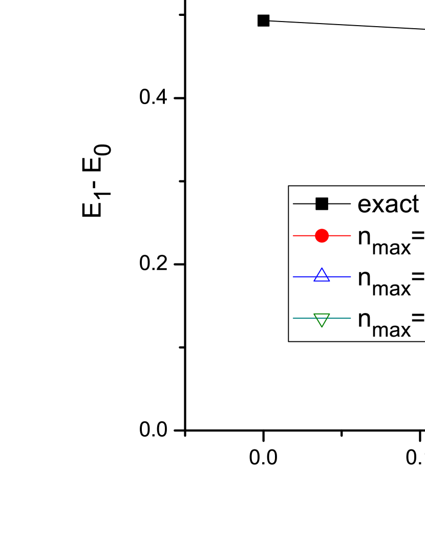
Figure 2: (Color online) The first excitation energy $E_{1}-E_{0}$ in the factorizable force model, as a function of the parameter $a=-b$, at the critical point $\omega=0$ ($\kappa=\kappa_{c}=1/16$). The black squares show the exact shell model results. The red circles are obtained by diagonalizing $\frac{\pi^{2}}{2}+\frac{1}{4}\cdot\frac{[1-2\cdot(a-b)^{2}]\alpha^{4}}{8}$ in the infinite phonon space. The blue triangles and the green inverted triangles are obtained by diagonalizing the same Hamiltonian in two different finite phonon spaces, specified by $n_{\rm{max}}$ and $u$; $u$ is the canonical transformation parameter defined in eq. (73), $n_{\rm{max}}$ is the maximal number of phonons.

As $a=-b$ increases, $\Lambda^{(40)}_{c}$ decreases. At some point $\Lambda^{(40)}_{c}$ becomes small numerically and $\frac{\pi^{2}}{2}+\frac{\Lambda_{c}^{(40)}\alpha^{4}}{4}$ no longer describes the behavior of the system near the critical point. First, other anharmonic terms, suppressed by powers of $1/\Omega$, may become important (see Appendix F). Second, even if there are no other anharmonicities, the description breaks down because the increasing zero-point-vibrations $\langle\alpha^{2}\rangle$ will exceed the range of the physical space, as discussed in Sec. IV.4. The current model has a larger vibrational amplitude than the Lipkin model due to a smaller $\Lambda^{(40)}_{c}$ ($\sim 1/\Omega$ verses $4/\Omega$). Fig. 2 shows $E_{1}-E_{0}$ as a function of the parameter $a=-b$ at the critical point $\omega=0$ ($\kappa=\kappa_{c}=1/16$). $E_{1}-E_{0}$ depends on the space in which we diagonalize $\frac{\pi^{2}}{2}+\frac{\Lambda_{c}^{(40)}\alpha^{4}}{4}$. Unlike in the Lipkin model, we do not know a priori what the physical space is in the current model. But it should be similar to that of the Lipkin model with $8$ particles. Thus we choose $n_{\rm{max}}=8$ for both two finite spaces, each with a reasonable $u$ of eq. (73). When $a=-b$ is small, say, less than $0.2$, $E_{1}-E_{0}$ of different spaces are close and all follow the trend of the exact $E_{1}-E_{0}$. When $a=-b$ is large, $E_{1}-E_{0}$ of different spaces differ substantially, implying that $\langle\alpha^{2}\rangle$ has reached the edge of the physical space, thus the bosonic approach becomes invalid. If in the current model we increase the collectivity $\Omega=N$, it is expected that $E_{1}-E_{0}$ from the GDM method will agree with the exact $E_{1}-E_{0}$ up to a larger value of $a=-b$.

In summary, near the critical point $\omega^{2}\approx 0$, the next even potential term $\Lambda^{(40)}$ dominates the dynamics of the system, provided it is positive and large. $\Lambda^{(40)}$ should be large enough such that other anharmonicities were negligible, and zero-point vibrations $\langle\alpha^{2}\rangle$ were within the finite physical boson space. A larger collectivity factor $\Omega$ helps both, since other anharmonicities are suppressed by powers of $\Omega^{-1}$ (see Appendix F), and the range of the physical space grows as $\Omega$.

VI Realistic Nuclear Application

There are three complications in realistic applications of the GDM method. A realistic nucleus has two kinds of fermions; symmetries, e.g. rotational invariance, need to be respected; pairing correlations should be considered.

As in the BCS theory we substitute the original system by a grand-canonical ensemble, in which the chemical potential is fixed by the average particle number of the ground state in the mean-field order. In this case we need to consider e.o.m. of not only $a_{2}^{\dagger}a_{1}$ but also $a_{2}a_{1}$. A good treatment of the superfluid ground state, on top of which collective excitations are formed, is essential.

The collective mode operators $\alpha_{\lambda\mu}$, $\pi_{\lambda\mu}$ have quantum numbers corresponding to symmetries of the Hamiltonian. In this section we keep only the quadrupole mode which is the most important one at low energy. The case of interacting modes (quadrupole and octupole) is discussed briefly in Appendix L.

This section is a straightforward generalization of Sec. II. The details of the derivation are given in Appendix G.

VI.1 Preparation

The microscopic fermionic Hamiltonian for the canonical ensemble is still given by eq. (1): we include the $-\mu\hat{N}$ term in $\hat{Z}$, and the s.p. index $1$, $2$ … can run over protons and neutrons. Isospin may not be conserved for some effective interactions. We do not write $V$ in the form $V^{J}_{(j_{1}j_{2}),(j_{3}j_{4})}$; $Z_{12}$ and $V_{1234}$ carry all the symmetries of $H$ implicitly.

Now the reference state $|\Phi\rangle$ does not have definite particle number,

$$\langle\Phi|a_{1}^{\dagger}a_{2}|\Phi\rangle\equiv\rho_{21},~{}~{}~{}\langle\Phi|a_{1}a_{2}|\Phi\rangle\equiv\kappa_{21}.$$ (102)

$\kappa$ is the pair correlator pair_correlator . Also we need two generalized density matrix operators

$$R_{12}\equiv a_{2}^{\dagger}a_{1},~{}~{}~{}K_{12}\equiv a_{2}a_{1},$$ (103)

and two self-consistent field operators

$$W\{R\}_{12}\equiv\sum_{34}V_{1432}R_{34},~{}~{}~{}f\{R\}\equiv Z+W\{R\},$$ (104)

$$\Delta\{K\}_{12}\equiv\frac{1}{2}\sum_{34}V_{1234}K_{43}.$$ (105)

It will be convenient to introduce ($R^{T}$, $f^{T}$ are transpose)

$$D\{R,K\}\equiv\left(\begin{array}[]{cc}R&K\\ K^{\dagger}&I-R^{T}\\ \end{array}\right),$$ (108)

$$S\{R,K\}\equiv\left(\begin{array}[]{cc}f\{R\}&\Delta\{K\}\\ \Delta^{\dagger}\{K\}&-f^{T}\{R\}\\ \end{array}\right).$$ (111)

The collective mode operators $\alpha^{\dagger}_{\lambda\mu}$, $\pi^{\dagger}_{\lambda\mu}$ carry quantum numbers of angular momentum $\lambda$, its projection $\mu$, and parity $(-)^{\lambda}$. The coordinate $\alpha^{\dagger}_{\lambda\mu}$ is time-even, and the momentum $\pi^{\dagger}_{\lambda\mu}$ is time-odd. Their Hermitian properties are

$$\alpha_{\lambda\mu}^{\dagger}=(-)^{\lambda-\mu}\alpha_{\lambda-\mu},~{}~{}~{}\pi_{\lambda\mu}^{\dagger}=(-)^{\lambda-\mu}\pi_{\lambda-\mu}.$$ (112)

The commutation relation is given by

$$[\alpha_{\lambda\mu}^{\dagger},\pi_{\lambda^{\prime}\mu^{\prime}}]=i~{}\delta_{\lambda\lambda^{\prime}}\delta_{\mu\mu^{\prime}}.$$ (113)

Here we consider only the quadrupole mode $\lambda=2$, and drop the label $\lambda$.

The collective Hamiltonian replacing eq. (4) should be written with correct vector coupling of the operators:

$$H=E_{0}+\frac{\omega^{2}}{2}\sqrt{5}(\alpha\times\alpha)^{0}_{0}+\frac{1}{2}\sqrt{5}(\pi\times\pi)^{0}_{0}$$

$$+\frac{\Lambda^{(30)}}{6}\sqrt{5}\{(\alpha\times\alpha)^{2},\alpha\}^{0}_{0}+\frac{\Lambda^{(12)}}{4}\sqrt{5}\{\alpha,(\pi\times\pi)^{2}\}^{0}_{0}$$

$$+\frac{\Lambda^{(40)}}{4}\sqrt{5}((\alpha\times\alpha)^{0}\times(\alpha\times\alpha)^{0})^{0}_{0}$$

$$+\frac{\Lambda^{(04)}}{4}\sqrt{5}((\pi\times\pi)^{0}\times(\pi\times\pi)^{0})^{0}_{0}$$

$$+\sum_{L=0,2,4}\frac{\Lambda^{(22)}_{L}}{8}\sqrt{5}\{(\alpha\times\alpha)^{L},(\pi\times\pi)^{L}\}^{0}_{0}.$$ (114)

$H$ is Hermitian, time-even, invariant under rotation and inversion.

VI.2 Equations of Motion in the Collective Band

Following the same procedure as in Sec. II, we find e.o.m. replacing those in Sec. II.2-II.5. Matrices $D^{(mn)}$, $S^{(mn)}$ are coefficients of expanding $D\{R,K\}$, $S\{R,K\}$ over collective operators $\alpha^{\dagger}_{\mu}$, $\pi^{\dagger}_{\mu}$. In the mean-field order we obtain the HFB equation

$$[S\{\rho,\kappa\},D\{\rho,\kappa\}]=[S^{(00)},D^{(00)}]=0.$$ (115)

In the harmonic order we obtain the QRPA equations

$$\underline{\pi^{\dagger}_{\mu}}:~{}~{}~{}~{}~{}~{}~{}~{}~{}iD^{(10)}_{\mu}=[S^{(00)},D^{(01)}_{\mu}]+[S^{(01)}_{\mu},D^{(00)}],$$ (116)

$$\underline{\alpha^{\dagger}_{\mu}}:~{}~{}-i\omega^{2}D^{(01)}_{\mu}=[S^{(00)},D^{(10)}_{\mu}]+[S^{(10)}_{\mu},D^{(00)}].$$ (117)

In the cubic order:

$$\underline{(\alpha^{\dagger}\times\alpha^{\dagger})^{L}_{\mu}/2,L=0,2,4:}~{}~{}~{}~{}~{}~{}~{}~{}~{}~{}~{}~{}~{}~{}~{}~{}~{}~{}~{}~{}~{}~{}~{}~{}~{}~{}~{}~{}~{}~{}$$

$$-2i\omega^{2}D^{(11)}_{L\mu}-2i\delta_{L,2}\Lambda^{(30)}D^{(01)}_{\mu}=$$

$${[}S^{(00)},D^{(20)}_{L\mu}]+[S^{(20)}_{L\mu},D^{(00)}]+2~{}[S^{(10)},D^{(10)}]^{L}_{\mu},~{}$$ (118)

$$\underline{(\pi^{\dagger}\times\pi^{\dagger})^{L}_{\mu}/2,L=0,2,4:}~{}~{}~{}~{}~{}~{}~{}~{}~{}~{}~{}~{}~{}~{}~{}~{}~{}~{}~{}~{}~{}~{}~{}~{}~{}~{}~{}~{}~{}~{}$$

$$2iD^{(11)}_{L\mu}-i\delta_{L,2}\Lambda^{(12)}D^{(01)}_{\mu}=$$

$${[}S^{(00)},D^{(02)}_{L\mu}]+[S^{(02)}_{L\mu},D^{(00)}]+2~{}[S^{(01)},D^{(01)}]^{L}_{\mu},~{}$$ (119)

$$\underline{\{\alpha^{\dagger},\pi^{\dagger}\}^{L}_{\mu}/2,L=0,1,2,3,4:}~{}~{}~{}~{}~{}~{}~{}~{}~{}~{}~{}~{}~{}~{}~{}~{}~{}~{}~{}~{}~{}~{}~{}~{}~{}~{}$$

$$-i\delta_{L,{\rm{even}}}\omega^{2}D^{(02)}_{L\mu}+i\delta_{L,{\rm{even}}}D^{(20)}_{L\mu}+i\delta_{L,2}\Lambda^{(12)}D^{(10)}_{\mu}$$

$$={[}S^{(00)},D^{(11)}_{L\mu}]+[S^{(11)}_{L\mu},D^{(00)}]$$

$$+[S^{(10)},D^{(01)}]^{L}_{\mu}-[D^{(10)},S^{(01)}]^{L}_{\mu}.~{}$$ (120)

In the quartic order:

$$\underline{\{(\alpha^{\dagger}\times\alpha^{\dagger})^{l_{L}},\alpha^{\dagger}\}^{L}_{\mu}/6,L=0,2,3,4,6:}~{}~{}~{}~{}~{}~{}~{}~{}$$

$$-\frac{3i}{2}\omega^{2}\sum_{l=0,2,4}D^{(21)}_{Ll\mu}\cdot\gamma^{L}_{l,l_{L}}-3i(-)^{L}\Lambda^{(30)}D^{(11)}_{L\mu}\cdot\gamma^{L}_{2,l_{L}}$$

$$-3i\delta_{L2}\Lambda^{(40)}D^{(01)}_{\mu}\cdot\gamma^{L=2}_{0,l_{L}}=[S^{(00)},D^{(30)}_{L}]+[S^{(30)}_{L},D^{(00)}]$$

$$+\frac{3}{2}\sum_{l=0,2,4}([S^{(20)}_{l},D^{(10)}]^{L}_{\mu}-[D^{(20)}_{l},S^{(10)}]^{L}_{\mu})\cdot\gamma^{L}_{l,l_{L}},~{}$$ (121)

$$\underline{\{(\alpha^{\dagger}\times\alpha^{\dagger})^{l},\pi^{\dagger}\}^{L}_{\mu}/4;l=0,2,4;L=0,1,2,3,4,5,6:}$$

$$-2i(-)^{L}\omega^{2}\sum_{l^{\prime}=0,2,4}D^{(12)}_{Ll^{\prime}\mu}\cdot g^{L}_{l,l^{\prime}}+\frac{2i}{3}~{}\delta_{l,l_{L}}D^{(30)}_{L\mu}$$

$$+\frac{4~{}i}{3}D^{(30)}_{L\mu}\cdot g^{L}_{l,l_{L}}-2i~{}\delta_{l2}~{}\Lambda^{(30)}D^{(02)}_{L\mu}$$

$$+2~{}i\Lambda^{(12)}D^{(20)}_{L\mu}\cdot g^{L}_{l,2}+i~{}\delta_{L2}~{}\Lambda^{(22)}_{l}D^{(10)}_{\mu}$$

$$=[S^{(00)},D^{(21)}_{Ll\mu}]+[S^{(21)}_{Ll\mu},D^{(00)}]$$

$$+[S^{(20)}_{l},D^{(01)}]^{L}_{\mu}-[D^{(20)}_{l},S^{(01)}]^{L}_{\mu}$$

$$+2\sum_{l^{\prime}=0,1,2,3,4}([S^{(11)}_{l^{\prime}},D^{(10)}]^{L}_{\mu}-[D^{(11)}_{l^{\prime}},S^{(10)}]^{L}_{\mu})\cdot g^{L}_{l,l^{\prime}},$$ (122)

$$\underline{\{\alpha^{\dagger},(\pi^{\dagger}\times\pi^{\dagger})^{l}\}^{L}_{\mu}/4;l=0,2,4;L=0,1,2,3,4,5,6:}$$

$$-\frac{2i}{3}\delta_{l,l_{L}}(-)^{L}\omega^{2}D^{(03)}_{L\mu}-\frac{4i}{3}\omega^{2}D^{(03)}_{L\mu}(-)^{L-l_{L}}\cdot g^{L}_{l,l_{L}}$$

$$+2i(-)^{L}\sum_{l^{\prime}=0,2,4}D^{(21)}_{Ll^{\prime}\mu}\cdot g^{L}_{l,l^{\prime}}-i\delta_{l2}\Lambda^{(12)}D^{(11)}_{L\mu}$$

$$+2i(-)^{L}\Lambda^{(12)}D^{(11)}_{L\mu}\cdot g^{L}_{l,2}-i~{}\delta_{L2}~{}\Lambda^{(22)}_{l}D^{(01)}_{\mu}$$

$$=[S^{(00)},D^{(12)}_{Ll\mu}]+[S^{(12)}_{Ll\mu},D^{(00)}]$$

$$+[S^{(10)},D^{(02)}_{l}]^{L}_{\mu}-[D^{(10)},S^{(02)}_{l}]^{L}_{\mu}$$

$$+2\sum_{l^{\prime}=0,1,2,3,4}([S^{(11)}_{l^{\prime}},D^{(01)}]^{L}_{\mu}-[D^{(11)}_{l^{\prime}},S^{(01)}]^{L}_{\mu})(-)^{L-l^{\prime}}g^{L}_{l,l^{\prime}},~{}~{}~{}$$ (123)

$$\underline{\{(\pi^{\dagger}\times\pi^{\dagger})^{l_{L}},\pi^{\dagger}\}^{L}_{\mu}/6,L=0,2,3,4,6:}~{}~{}~{}~{}~{}~{}~{}~{}~{}~{}~{}~{}~{}~{}~{}~{}~{}~{}~{}~{}~{}$$

$$\frac{3i}{2}(-)^{L}\sum_{l=0,2,4}D^{(12)}_{Ll\mu}\cdot\gamma^{L}_{l,l_{L}}-\frac{3i}{2}\Lambda^{(12)}D^{(02)}_{L\mu}\cdot\gamma^{L}_{2,l_{L}}$$

$$+3i\delta_{L2}\Lambda^{(04)}D^{(10)}_{\mu}\cdot\gamma^{L=2}_{0,l_{L}}=[S^{(00)},D^{(03)}_{L}]+[S^{(03)}_{L},D^{(00)}]$$

$$+\frac{3}{2}\sum_{l=0,2,4}([S^{(02)}_{l},D^{(01)}]^{L}_{\mu}-[D^{(02)}_{l},S^{(01)}]^{L}_{\mu})\cdot\gamma^{L}_{l,l_{L}}.~{}~{}$$ (124)

The numerical coefficients $\gamma^{L}_{l,l^{\prime}}$ and $g^{L}_{l,l^{\prime}}$ are defined by

$$\{(\alpha\times\alpha)^{l},\alpha\}^{L}_{\mu}=\gamma^{L}_{l,l^{\prime}}\cdot\{(\alpha\times\alpha)^{l^{\prime}},\alpha\}^{L}_{\mu},~{}(\gamma^{L}_{l,l}=1),$$ (125)

$$\frac{1}{8}\{\{\alpha,\pi\}^{l^{\prime}},\alpha\}^{L}_{\mu}=\sum_{l=0,2,4}g^{L}_{l,l^{\prime}}\cdot\frac{1}{4}\{(\alpha\times\alpha)^{l},\pi\}^{L}_{\mu}.~{}$$ (126)

Values of $\gamma^{L}_{l,l^{\prime}}$ and $g^{L}_{l,l^{\prime}}$ are given in Appendix I. $l_{L}$ in $\{(\alpha^{\dagger}\times\alpha^{\dagger})^{l_{L}},\alpha^{\dagger}\}^{L}_{\mu}/6$ is the choice of basis, different choices of $l_{L}$ do not influence results.

There exists a relation involving cubic and quartic anharmonicities, replacing eq. (57). Setting $L=2$, keeping only $(D/S)^{(30/21/12/03)}$ and $\Lambda^{(40)}$, $\Lambda^{(22)}_{l}$, $\Lambda^{(04)}$ terms, $f_{l_{L}}\times$ eq. (121) $+\frac{1}{2}\omega^{2}\sum_{l=0,2,4}f_{l}\times$ eq. (123) gives

$$\underline{L=2:}~{}~{}~{}-i\omega^{2}\cdot\Big{(}~{}\frac{1}{2}\sum_{l=0,2,4}f_{l}\cdot D^{(21)}_{Ll\mu}+\omega^{2}f_{l_{L}}\cdot D^{(03)}_{L\mu}~{}\Big{)}$$

$$=[~{}S^{(00)}~{},~{}\Big{(}~{}f_{l_{L}}\cdot D^{(30)}_{L}+\frac{1}{2}\omega^{2}\sum_{l=0,2,4}f_{l}\cdot D^{(12)}_{Ll\mu}~{}\Big{)}~{}]$$

$$+[~{}\Big{(}~{}f_{l_{L}}\cdot S^{(30)}_{L}+\frac{1}{2}\omega^{2}\sum_{l=0,2,4}f_{l}\cdot S^{(12)}_{Ll\mu}~{}\Big{)}~{},~{}D^{(00)}~{}]$$

$$+3i\Lambda^{(40)}D^{(01)}_{\mu}\cdot f_{0}+\frac{i}{2}\omega^{2}\sum_{l=0,2,4}f_{l}\cdot\Lambda^{(22)}_{l}D^{(01)}_{\mu}+\ldots~{}~{}~{}$$ (127)

$\frac{1}{2}\sum_{l=0,2,4}f_{l}\times$ eq. (122) $+\omega^{2}f_{l_{L}}\times$ eq. (124) gives

$$\underline{L=2:}~{}~{}~{}~{}~{}~{}~{}~{}~{}i\cdot\Big{(}~{}f_{l_{L}}\cdot D^{(30)}_{L\mu}+\frac{1}{2}\omega^{2}\sum_{l=0,2,4}f_{l}\cdot D^{(12)}_{Ll\mu}~{}\Big{)}$$

$$=[~{}S^{(00)}~{},~{}\Big{(}~{}\frac{1}{2}\sum_{l=0,2,4}f_{l}\cdot D^{(21)}_{Ll\mu}+\omega^{2}f_{l_{L}}\cdot D^{(03)}_{L}~{}\Big{)}~{}]$$

$$+[~{}\Big{(}~{}\frac{1}{2}\sum_{l=0,2,4}f_{l}\cdot S^{(21)}_{Ll\mu}+\omega^{2}f_{l_{L}}\cdot S^{(03)}_{L}~{}\Big{)}~{},~{}D^{(00)}~{}]$$

$$-\frac{i}{2}\sum_{l=0,2,4}f_{l}\cdot\Lambda^{(22)}_{l}D^{(10)}_{\mu}-3i\omega^{2}\Lambda^{(04)}D^{(10)}_{\mu}\cdot f_{0}+\ldots~{}~{}~{}$$ (128)

where $f_{l}$ is defined in eq. (284). A solvability condition exists because the variable parts of eqs. (127) and (128) have the same structure as the QRPA equations (116) and (117).

Following the procedure in Sec. III, we can obtain expressions of $\Lambda^{(30)}_{c}$ and $\Lambda^{(40)}_{c}$. In the next section we do this explicitly for the quadrupole plus pairing model.

VII Quadrupole plus Pairing Model

In this section the GDM method is applied to the quadrupole plus pairing Hamiltonian. As was understood long ago P_Q1 ; P_Q2 , this model combines the most important nuclear collective phenomena in particle-particle (pairing) and particle-hole (quadrupole mode) channels. The approximate analytical results of the GDM method are compared below with the exact results of the shell model diagonalization. The operator of multiple moment is defined as

$$Q^{\dagger}_{\lambda\mu}\{R\}=Tr\{q^{\dagger}_{\lambda\mu}R\}=\sum_{12}q^{\dagger}_{\lambda\mu 12}a_{1}^{\dagger}a_{2},$$ (129)

$$q_{\lambda\mu}^{\dagger}=f_{\lambda}(r)\cdot i^{\lambda}~{}Y_{\lambda\mu}(\theta,\phi),$$ (130)

where $f_{\lambda}(r)$ is real. The definition of eq. (130) differs from the “usual” one in two aspects: a factor $i^{\lambda}$ is included, and $q_{\lambda\mu}^{\dagger}\sim Y_{\lambda\mu}$ instead of $q_{\lambda\mu}$, thus $q_{\lambda\mu}^{\dagger}$ creates projection $\mu$. The Hermitian properties are

$$q^{\dagger}_{\lambda\mu}=(-)^{\lambda-\mu}q_{\lambda\mu},~{}~{}~{}Q^{\dagger}_{\lambda\mu}=(-)^{\lambda-\mu}Q_{\lambda\mu}.$$ (131)

The pairing operators $P$ and $P^{\dagger}$ are defined by

$$P^{\dagger}=\frac{1}{2}\sum_{1}a_{1}^{\dagger}a_{\tilde{1}}^{\dagger},~{}~{}~{}P=\frac{1}{2}\sum_{1}a_{\tilde{1}}a_{1},$$ (132)

where $\tilde{1}$ is the time-reversed s.p. level of $1$. $P$ has angular momentum $0$ and positive parity. $P+P^{\dagger}$ is time-even, $P-P^{\dagger}$ is time-odd.

The quadrupole plus pairing Hamiltonian is (dropping $\lambda=2$)

$$H=\sum_{1}(\epsilon_{1}-\mu)a_{1}^{\dagger}a_{1}-\frac{G}{4}\sum_{12}a_{1}^{\dagger}a_{\tilde{1}}^{\dagger}a_{\tilde{2}}a_{2}$$

$$+\frac{1}{4}\sum_{1234}\sum_{\mu}(-\kappa~{}q^{\dagger}_{\mu 14}q_{\mu 23}+\kappa~{}q^{\dagger}_{\mu 13}q_{\mu 24})a_{1}^{\dagger}a_{2}^{\dagger}a_{3}a_{4}.$$ (133)

Approximately, this Hamiltonian can be written as $H\approx\sum_{1}(\epsilon_{1}-\mu)a_{1}^{\dagger}a_{1}-GP^{\dagger}P-\frac{1}{2}\kappa\sum_{\mu}Q_{\mu}^{\dagger}Q_{\mu}$. The difference is in a one-body term originating from the $Q\cdot Q$ part. $H$ is Hermitian and time-even, which implies real $G$, $\kappa$, $\epsilon_{1}=\epsilon_{\tilde{1}}$. In a realistic nucleus there are protons and neutrons; formally we can still use eq. (133) if the quadrupole force strengths are the same for proton-proton, neutron-neutron, and proton-neutron ($\kappa_{p}=\kappa_{n}=\kappa_{pn}=\kappa$), while remembering the pairing is treated for protons and neutrons separately ($G_{p}\neq G_{n}$). We will assume this is the case.

VII.1 The GDM Method

VII.1.1 BCS

In the pairing plus quadrupole model the HFB equation (115) becomes the BCS equation:

$$\Delta\cdot\Big{(}~{}1-\frac{G}{4}\sum_{1}\frac{1}{E_{1}}~{}\Big{)}=0,$$ (134)

$$e_{1}=\epsilon_{1}-\mu-G(v_{1})^{2},$$ (135)

$$E_{1}=\sqrt{(e_{1})^{2}+(\Delta)^{2}},$$ (136)

$$(u_{1})^{2}=\frac{1}{2}~{}(1+\frac{e_{1}}{E_{1}}),~{}~{}~{}(v_{1})^{2}=\frac{1}{2}~{}(1-\frac{e_{1}}{E_{1}}),$$ (137)

$$N=\sum_{1}(v_{1})^{2}.$$ (138)

BCS amplitudes $u_{1}=u_{\tilde{1}}$, $v_{1}=v_{\tilde{1}}$ are real. Pairing energy $\Delta$ is a real number, not to be confused with the field $\Delta\{K\}$ in eq. (105) that is an operator matrix. $E_{1}$ is the quasiparticle energy. The chemical potential $\mu$ is fixed by eq. (138). The gap equation (134) has a non-trivial solution $\Delta>0$ only if $G$ is greater than its critical value $G_{c}$ P_Q2 . For convenience we introduce:

$$\xi^{(2)}_{\mu 12}\equiv\frac{(u_{1}v_{2}+u_{2}v_{1})}{(E_{1}+E_{2})^{2}}q_{\mu 12},~{}\eta_{\mu 12}\equiv(u_{1}u_{2}-v_{1}v_{2})q_{\mu 12}.~{}~{}~{}$$ (139)

VII.1.2 QRPA

The QRPA secular equation corresponding to eq. (94) is given by

$$1=\kappa\sum_{12}\frac{(E_{1}+E_{2})~{}|\xi_{\mu 21}|^{2}}{(E_{1}+E_{2})^{2}-\omega^{2}}.$$ (140)

The solution $\omega^{2}$ is independent of $\mu$. Results in the form of reduced matrix elements are given in Appendix K. The normalization condition corresponding to eq. (95) is

$$1=(\kappa Q^{(10)})^{2}~{}\sum_{12}\frac{(E_{1}+E_{2})~{}|\xi_{\mu 21}|^{2}}{[(E_{1}+E_{2})^{2}-\omega^{2}]^{2}}.$$ (141)

VII.1.3 Cubic Anharmonicity

The cubic anharmonicity corresponding to eq. (96) is

$$\Lambda^{(30)}\doteq 3(\kappa Q^{(10)})^{3}\sum_{n_{1}j_{1}n_{2}j_{2}n_{3}j_{3}}$$

$$\sqrt{\frac{(2j_{1}+1)(2j_{2}+1)(2j_{3}+1)}{5}}\cdot\left\{\begin{array}[]{ccc}2&2&2\\ j_{1}&j_{2}&j_{3}\\ \end{array}\right\}$$ (144)

$$\cdot~{}\xi^{(1)\dagger}_{\|12}~{}\xi^{{(1)}\dagger}_{\|23}~{}\eta^{\dagger}_{\|31},$$ (145)

where $\xi^{(1)\dagger}_{\|12}\equiv\langle n_{1}j_{1}\|\xi^{(1)\dagger}\|n_{2}j_{2}\rangle$ is the reduced matrix element, the convention for which is given in Appendix J. $n_{1}$ combines all other quantum numbers specifying a s.p. level, except $j_{1}$.

We give the expression of $P^{(20)}$ which will appear in $\Lambda^{(40)}_{c}$:

$$P^{(20)}\cdot[~{}1-G\sum_{n_{1}j_{1}}(2j_{1}+1)\frac{[(u_{1})^{2}-(v_{1})^{2}]^{2}}{4E_{1}}~{}]\doteq$$

$$-(\kappa Q^{(10)})^{2}\sum_{n_{1}j_{1}n_{2}j_{2}}(2j_{1}+1)\cdot\sqrt{2j_{2}+1}\left\{\begin{array}[]{ccc}2&2&0\\ j_{1}&j_{1}&j_{2}\\ \end{array}\right\}$$ (148)

$$\cdot~{}\Big{[}~{}2u_{1}v_{1}\cdot\xi^{{(1)}\dagger}_{\|12}\xi^{{(1)}\dagger}_{\|21}-~{}\frac{(u_{1})^{2}-(v_{1})^{2}}{E_{1}}\cdot\eta^{\dagger}_{\|12}\xi^{{(1)}\dagger}_{\|21}~{}\Big{]}.~{}~{}~{}$$ (149)

$P^{(20)}$ is divergent when $G$ is greater than but close to $G_{c}$. In this region of the pairing phase transition, $\Delta$ is small, and $P^{(20)}\sim 1/\Delta$. The GDM $+$ BCS method is not valid in this region: in the mean-field order the BCS solution already fails, as is well known.

VII.1.4 Quartic Anharmonicity

The quartic anharmonicity corresponding to eq. (98) is

$$f_{0}\cdot\Lambda^{(40)}\doteq-2~{}f_{2}\cdot(\kappa Q^{(10)})^{2}(\Lambda^{(30)})^{2}~{}{\rm{Tr}}\Big{[}\xi_{\mu}\xi^{{(5)}\dagger}_{\mu}\Big{]}$$

$$-f_{2}\cdot\Lambda^{(30)}\Lambda^{(12)}$$

$$-f_{2}\cdot\Lambda^{(30)}(\kappa Q^{(10)})^{3}\Big{(}~{}{\rm{Tr}}\Big{[}\{\xi^{(1)},\xi^{(3)}\}^{L=2}_{\mu}\eta^{\dagger}_{\mu}\Big{]}$$

$$+{\rm{Tr}}\Big{[}\{\eta,\xi^{(3)}\}^{L=2}_{\mu}\xi^{{(1)}\dagger}_{\mu}\Big{]}+2~{}{\rm{Tr}}\Big{[}\{\eta,\xi^{(1)}\}^{L=2}_{\mu}\xi^{{(3)}\dagger}_{\mu}\Big{]}$$

$$+{\rm{Tr}}\Big{[}\{\eta,\xi^{{(2)}}\}^{L=2}_{\mu}\xi^{{(2)}\dagger}_{\mu}\Big{]}~{}\Big{)}$$

$$-f_{0}\cdot G~{}P^{(20)}(\kappa Q^{(10)})^{2}~{}\sum_{12}(u_{1}v_{1}+u_{2}v_{2})~{}\xi_{\mu 12}\xi^{{(2)}\dagger}_{\mu 21}$$

$$+f_{0}\cdot G~{}P^{(20)}(\kappa Q^{(10)})^{2}$$

$$\cdot\sum_{12}\{\frac{(u_{1})^{2}-(v_{1})^{2}}{2E_{1}}+\frac{(u_{2})^{2}-(v_{2})^{2}}{2E_{2}}\}\xi^{(1)}_{\mu 12}\eta^{\dagger}_{\mu 21}$$

$$+(\kappa Q^{(10)})^{4}\sum_{l=0,2,4}f_{l}\cdot\Big{(}{\rm{Tr}}\Big{[}\{\xi,(\xi^{(1)}\times\xi^{(1)})^{l}\}^{L=2}_{\mu}\xi^{{(1)}\dagger}_{\mu}\Big{]}$$

$$-{\rm{Tr}}\Big{[}\{\eta,\{\eta,\xi^{{(1)}}\}^{l,(1)}\}^{L=2}_{\mu}\xi^{{(1)}\dagger}_{\mu}\Big{]}$$

$$-{\rm{Tr}}\Big{[}\{\xi^{(1)},\{\eta,\xi^{{(1)}}\}^{l,(1)}\}^{L=2}_{\mu}\eta^{\dagger}_{\mu}\Big{]}~{}\Big{)},$$ (150)

where $\{\eta,\xi^{(1)}\}^{l,(1)}_{12}=\{\eta,\xi^{(1)}\}^{l}_{12}/(E_{1}+E_{2})$. There is an undetermined parameter $\Lambda^{(12)}$ in eq. (150). Values of numerical factors $f_{l}$ are given in Appendix I.

VII.2 Comparison with Exact Results

We compare the results of our method in a semi-realistic model with those of NuShellX MSU_Nu . There are $10$ fermions of one kind and four s.p. levels with energies:

$$\left.\begin{array}[]{c|c|c|c|c}{\rm{s.p.~{}levels}}&1p\frac{1}{2}&0f\frac{7}{2}&1p\frac{3}{2}&0f\frac{5}{2}\\ \epsilon~{}{\rm{(MeV)}}&-0.1&0.0&1.0&1.1\\ \end{array}\right.$$ (153)

We take the radial wavefunctions to be harmonic oscillator ones. In eq. (130) we take $f(r)$ to be $r^{2}$ so $q^{\dagger}_{\mu}=-\hat{r}^{2}Y_{2\mu}(\hat{\theta},\hat{\phi})$. For convenience we make $q^{\dagger}_{\mu}$ dimensionless by combining its original dimension with $\kappa$ (see the end of Appendix J). The model space is similar to the realistic $pf$-shell, but the $1p\frac{1}{2}$ and $1p\frac{3}{2}$ levels are inverted to increase collectivity: in the current case the $q$ matrix elements ($q_{1p\frac{1}{2},0f\frac{5}{2}}$ and $q_{1p\frac{3}{2},0f\frac{7}{2}}$) are large between the s.p. levels above and below the Fermi surface.

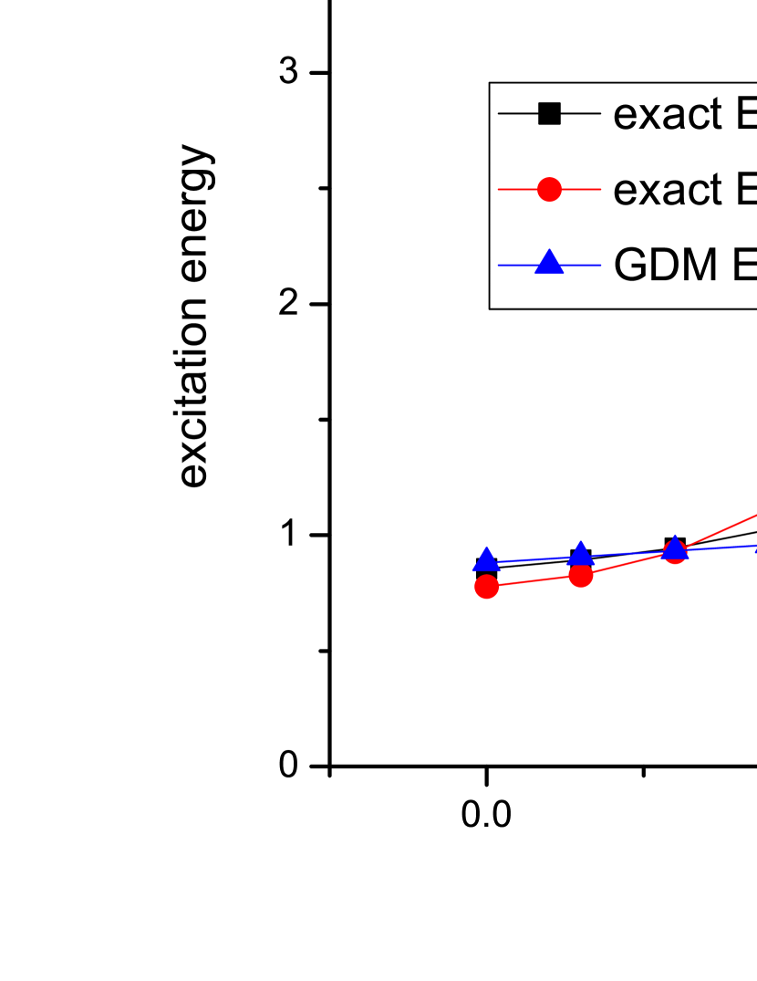
Figure 3: (Color online) Excitation energies (from Table 2) in the quadrupole plus pairing model as a function of the pairing strength $G$, at the critical point $\omega=0$ ($\kappa=\kappa_{c}$). The black squares and red circles show the exact excitation energy of the first $2^{+}$ and $4^{+}$ state, respectively, “NuShellX $E_{2_{1}^{+}}$” and “NuShellX $E_{4_{1}^{+}}$” in Table 2. The blue triangles give “GDM $E_{2^{+}}$” from Table 2.

We did a set of calculations with increasing pairing strength $G$. At each value of $G$, the strength $\kappa$ of the $Q\cdot Q$ force is taken to be at the critical value $\kappa_{c}$ such that the RPA frequency $\omega^{2}=0$. The results are summarized in Table 2. For clarity, we draw the last three lines of Table 2 as Fig. 3. The coefficient $\Lambda^{(40)}$ in Table 2 is calculated by eq. (150) setting $\Lambda^{(12)}=0$ (dropping the $-f_{2}\cdot\Lambda^{(30)}\Lambda^{(12)}$ term). A non-zero term $\Lambda^{(12)}$ in its reasonable range does not influence $\Lambda^{(40)}$ much, since in the current model $\Lambda^{(30)}$ is small due to the approximate symmetry with respect to the Fermi surface (see Table 2). Then “GDM $E_{2^{+}}$” is calculated by diagonalizing eq. (114), setting $\Lambda^{(12)}=\Lambda^{(04)}=\Lambda^{(22)}_{L}=0$ ($\omega^{2}=0$ since $\kappa$ takes its critical value).

The critical value of the pairing strength $G_{c}$ is around $0.11\sim 0.12$ MeV. When $G<G_{c}$, the BCS solution $\Delta=0$, and $\mu$ can be anywhere between $\epsilon_{0f\frac{7}{2}}=0$ and $\epsilon_{1p\frac{3}{2}}=1.0$ MeV. We checked that in this case our results (140-150) do not depend on the choice of $\mu$. In Table 2 we fix $\mu$ at $0.5$ MeV. In the region where $G$ is greater than but close to $G_{c}$, our method is invalid as discussed under eq. (149). This is illustrated in Fig. 3 by the ‘kink’ on the “GDM $E_{2^{+}}$” curve near $G\sim 0.12$.

In Fig. 3 “exact $E_{2^{+}}$” and “exact $E_{4^{+}}$” are the exact results by NuShellX. At $G=0$ the first excited state is $4^{+}$ instead of $2^{+}$. In this case the $4^{+}$ state is a single-particle excitation from $0f\frac{7}{2}$ to $0f\frac{5}{2}$; the $2^{+}$ state is a collective state with approximately half holes in $1p\frac{1}{2}$ and $0f\frac{7}{2}$ levels, half particles in $1p\frac{3}{2}$ and $0f\frac{5}{2}$. As $G$ increases, the collective $2^{+}$ state becomes the first excited state. When $G$ is large enough, $\Delta$ dominates over the original s.p. spacing $\epsilon$, and the results become stable. As an example, at $G=0.30$ MeV, the quasiparticle continuum starts at $\sim 3.5$ MeV; from the second excited state $0^{+}$ at $3.506$ MeV to $4.153$ MeV there are $15$ states with $J^{P}=0^{+},2^{+},4^{+},6^{+}$. The first excited state $2^{+}$ at $2.438$ MeV should be identified as a collective state, stabilized at around sixty percents within the gap.

It is seen in Fig. 3 that “GDM $E_{2^{+}}$” agrees well with the exact result “exact $E_{2^{+}}$” in general. On the $G<G_{c}$ side, our $E_{2^{+}}$ does increase with $G$ although not rapidly enough. On the $G>G_{c}$ side, when $\Delta$ is not too small, the agreement is very good.

In summary, this section shows the potential of the GDM method in doing realistic calculations. In medium and heavy nuclei the pairing gap $\sim 2\Delta\sim 2$ MeV, the critical region is approximately bounded by $|\omega|<1~{}{\rm{MeV}}$. Nuclei on the $\omega^{2}<0$ side are gamma-unstable. On the $\omega^{2}>0$ side, the whole region can be calculated as in Fig. 1 [explained in the paragraph under eq. (101)].

VIII Conclusions

The GDM method is promising in solving the longstanding problem: constructing the collective bosonic Hamiltonian microscopically. The procedure is straightforward and consistent. Results of the lowest orders, the well-known HFB and QRPA equations, give us confidence to proceed to higher order anharmonicities. The anharmonicities are important as the harmonic potential $\omega^{2}\alpha^{2}/2$ becomes small or negative when going away from closed shells. The GDM method provides a unified description of different collective phenomena, including soft vibrational modes of large amplitudes, gamma-unstable potential and transition to static deformation. It maps the exact fermionic e.o.m. onto the dynamics generated by approximate collective operators. Here we used the phonon-like operators; other possibilities include rotational dynamics and the dynamics corresponding to the symplectic symmetry or other group-theoretical models. In such cases the GDM expansion should be based on the group generators.

Sec. II discusses the general procedure of the GDM method. In each order, a set of coupled linear equations is solved in terms of lower order results. At the current stage the anharmonicities are not completely fixed; we find only one relation (57) involving the cubic and quartic anharmonicities, appearing in the third order as a solvability condition. In Sec. III it is shown that around the critical point $\omega^{2}\approx 0$, we are able to determine the cubic potential $\Lambda^{(30)}$ (66) and the quartic potential $\Lambda^{(40)}$ (68). $\Lambda^{(40)}$ should be responsible for restoring the stability of the system near the critical point, if it is positive and large. This idea is then tested in three models of increasing complexity: the Lipkin model (Sec. IV), model with factorizable forces (Sec. V), and the quadrupole plus pairing model (Sec. VII). The GDM method is only responsible for calculating $\Lambda^{(mn)}$; other conditions are needed if the resultant bosonic Hamiltonian is used to reproduce the spectrum of the original fermionic Hamiltonian, as discussed in the last two paragraphs of Sec. IV.4. If these conditions are not fulfilled, the approach of effective bosonic Hamiltonian encounters serious difficulties. The conditions for quartic potential ($\Lambda^{(40)}\alpha^{4}/4$) dominance near the critical point are discussed in the last paragraph of Sec. V.2.

Calculations for realistic nuclei are in progress. However, the pairing correlations need to be treated better than in the BCS framework, because anharmonicities are sensitive to the occupation numbers ($u_{1}$, $v_{1}$) of the superfluid ground state. Unlike the QRPA secular equation (140), where terms in the summation contribute coherently, in the expressions of anharmonicities (145) and (150) different terms may cancel. $\Lambda^{(30)}$ and $\Lambda^{(40)}$ depend on the balancing above and below the Fermi surface, thus they are sensitive to the occupation numbers ($u_{1}$, $v_{1}$). Work is also in progress about the role of $\Lambda^{(30)}$ on deformation, as well as the quadrupole-octupole coupling in the presence of a low-lying octupole mode. The realistic effective interactions (better than the quadrupole plus pairing Hamiltonian) are to be used in the calculation. The present paper sets the scene for the GDM method in the sense that it is seen explicitly there are no contradictions in the solutions (Sec. II and VI), although at the current stage we find only one constraint (57) on the anharmonicities. New constraints, if found, would fix the anharmonicities completely.

Acknowledgements: The author gratefully expresses many thanks to his advisor Vladimir Zelevinsky, who provided superior guidance and help during the whole work. Support from the NSF grant PHY-0758099 is acknowledged. The author is also thankful to the National Superconducting Cyclotron Laboratory and Department of Physics and Astronomy at Michigan State University.

Appendix A Three-Body Force

It is straightforward to include three-body forces in the formulation. The microscopic Hamiltonian (1) includes a new (anti-symmetrized) term

$$H^{(3)}=\frac{1}{36}\sum_{123456}G_{123456}a_{1}^{\dagger}a_{2}^{\dagger}a_{3}^{\dagger}a_{4}a_{5}a_{6}.$$ (154)

Under the definition

$$G\{R\}_{1256}\equiv\sum_{34}G_{123456}R_{43},$$

$$G\{R,R\}_{14}\equiv\sum_{23}G\{R\}_{1234}R_{32},$$ (155)

the normal ordering Hamiltonian (10) acquires new terms,

$$\langle\Phi|H^{(3)}|\Phi\rangle=\frac{1}{6}{\rm{Tr}}[G\{\rho,\rho\}\rho],$$

$$f^{(3)}=\frac{1}{2}G\{\rho,\rho\},~{}~{}~{}V^{(3)}=G\{\rho\},$$ (156)

and a term $\frac{1}{36}\sum_{123456}G_{123456}N[a_{1}^{\dagger}a_{2}^{\dagger}a_{3}^{\dagger}a_{4}a_{5}a_{6}]$. In the e.o.m. (12) $f$ and $V$ are replaced by the new ones including $f^{(3)}$ and $V^{(3)}$ ($W\{R\}$ is calculated from the new $V$), and there are two additional terms:

$$+\frac{1}{4}[G\{R^{2N}\},\rho]_{12}+\frac{1}{12}\sum_{34567}(G_{134567}N[a_{2}^{\dagger}a_{3}^{\dagger}a_{4}^{\dagger}a_{5}a_{6}a_{7}]$$

$$-G_{765432}N[a_{7}^{\dagger}a_{6}^{\dagger}a_{5}^{\dagger}a_{4}a_{3}a_{1}]),~{}~{}$$ (157)

where

$$G\{R^{2N}\}_{16}\equiv\sum_{2345}G_{123456}N[a_{2}^{\dagger}a_{3}^{\dagger}a_{4}a_{5}].$$ (158)

Formally the HF and RPA equations are the same as before, replacing $f$ and $W\{R\}$ by the new ones.

Appendix B Saturation Principle for Section II

Keeping only one-body terms in $\alpha$ and $\pi$,

$$\alpha=\sum_{12}x_{12}R_{21}=\sum_{12}x_{12}a_{1}^{\dagger}a_{2},$$ (159)

$$\pi=\sum_{12}p_{12}R_{21}=\sum_{12}p_{12}a_{1}^{\dagger}a_{2},$$ (160)

we have the following identities in the full space:

$$[R_{12},\alpha]=[x,R]_{12},$$ (161)

$${[}R_{12},\pi]=[p,R]_{12},$$ (162)

where $[x,R]_{12}=\sum_{3}(x_{13}R_{32}-R_{13}x_{32})$. Similarly to the manipulation of eq. (12), we project eqs. (161,162) onto the collective subspace. Since $\alpha$ and $\pi$ are collective operators, we can substitute $R$ by its boson expansion (14). After calculating commutators on the l.h.s. , we equate coefficients of the same phonon structure: $1$, $\alpha$, $\pi$, $\frac{\alpha^{2}}{2}$ … Eq. (161) gives

$$-ir^{(01)}_{12}=[x,\rho]_{12}=x_{12}(n_{2}-n_{1}),$$ (163)

$$-ir^{(02)}={[x,r^{(01)}]},~{}~{}~{}-ir^{(11)}={[x,r^{(10)}]}.$$ (164)

Eq. (162) gives

$$ir^{(10)}_{12}=[p,\rho]_{12}=p_{12}(n_{2}-n_{1}),$$ (165)

$$ir^{(20)}={[p,r^{(10)}]},~{}~{}~{}ir^{(11)}={[p,r^{(01)}]}.$$ (166)

Only the $n_{1}\neq n_{2}$ matrix elements of $x$ and $p$ are determined from eqs. (163) and (165). Higher order expressions (164) and (166) are approximate, saying that $r^{(20/11/02)}$ are completely fixed by the the harmonic order solutions. In fact the two expressions of $r^{(11)}$ are not consistent with each other. These defects are due to the neglected many-body components in eqs. (159) and (160), as explained in Appendix C. The approximate expressions (164) and (166) are used below to derive expressions of $r^{(mn)}_{1234}$ in terms of $r^{(mn)}_{12}$.

In the full space we also have

$$[N[a_{4}^{\dagger}a_{3}^{\dagger}a_{2}a_{1}],\alpha]=$$

$$-\sum_{5}x_{25}N[a_{4}^{\dagger}a_{3}^{\dagger}a_{1}a_{5}]+\sum_{5}x_{15}N[a_{4}^{\dagger}a_{3}^{\dagger}a_{2}a_{5}]$$

$$-\sum_{6}x_{64}N[a_{6}^{\dagger}a_{3}^{\dagger}a_{2}a_{1}]+\sum_{6}x_{63}N[a_{6}^{\dagger}a_{4}^{\dagger}a_{2}a_{1}]$$

$$+ir^{(01)}_{24}N[a_{3}^{\dagger}a_{1}]-ir^{(01)}_{23}N[a_{4}^{\dagger}a_{1}]$$

$$-ir^{(01)}_{14}N[a_{3}^{\dagger}a_{2}]+ir^{(01)}_{13}N[a_{4}^{\dagger}a_{2}],$$ (167)

where we have used eq. (163). Similarly

$$[N[a_{4}^{\dagger}a_{3}^{\dagger}a_{2}a_{1}],\pi]=$$

$$-\sum_{5}p_{25}N[a_{4}^{\dagger}a_{3}^{\dagger}a_{1}a_{5}]+\sum_{5}p_{15}N[a_{4}^{\dagger}a_{3}^{\dagger}a_{2}a_{5}]$$

$$-\sum_{6}p_{64}N[a_{6}^{\dagger}a_{3}^{\dagger}a_{2}a_{1}]+\sum_{6}p_{63}N[a_{6}^{\dagger}a_{4}^{\dagger}a_{2}a_{1}]$$

$$-ir^{(10)}_{24}N[a_{3}^{\dagger}a_{1}]+ir^{(10)}_{23}N[a_{4}^{\dagger}a_{1}]$$

$$+ir^{(10)}_{14}N[a_{3}^{\dagger}a_{2}]-ir^{(10)}_{13}N[a_{4}^{\dagger}a_{2}],$$ (168)

where we have used eq. (165). Again we project eqs. (167) and (168) onto the collective subspace, then substitute the expansions (14) and (15). Both the l.h.s. and the r.h.s. have no constant terms. This justifies the assumption under eq. (15): terms linear in $\alpha$ and $\pi$ are absent in the expansion (15) of $N[a_{4}^{\dagger}a_{3}^{\dagger}a_{2}a_{1}]$, since they generate constant terms in the l.h.s. of eqs. (167) and (168). The $\alpha$ and $\pi$ terms of eqs. (167) and (168) give

$$r^{(20)}_{1234}=r^{(10)}_{14}r^{(10)}_{23}-r^{(10)}_{13}r^{(10)}_{24}-r^{(10)}_{24}r^{(10)}_{13}+r^{(10)}_{23}r^{(10)}_{14},~{}~{}~{}$$ (169)

$$r^{(02)}_{1234}=r^{(01)}_{14}r^{(01)}_{23}-r^{(01)}_{13}r^{(01)}_{24}-r^{(01)}_{24}r^{(01)}_{13}+r^{(01)}_{23}r^{(01)}_{14},~{}~{}~{}$$ (170)

$$r^{(11)}_{1234}=r^{(10)}_{14}r^{(01)}_{23}-r^{(10)}_{13}r^{(01)}_{24}-r^{(10)}_{24}r^{(01)}_{13}+r^{(10)}_{23}r^{(01)}_{14}.~{}~{}~{}~{}$$ (171)

We mention that eq. (167) and (168) give the same expression of $r^{(11)}_{1234}$ (171). Using eqs. (164), (166) and (169-171), the $\alpha^{2}/2$, $\{\alpha,\pi\}/2$, $\pi^{2}/2$ terms of eqs. (167) and (168) give

$$r^{(30)}_{1234}=\frac{3}{2}(r^{(20)}_{14}r^{(10)}_{23}-r^{(20)}_{13}r^{(10)}_{24}-r^{(20)}_{24}r^{(10)}_{13}+r^{(20)}_{23}r^{(10)}_{14}),~{}~{}~{}$$ (172)

$$r^{(03)}_{1234}=\frac{3}{2}(r^{(02)}_{14}r^{(01)}_{23}-r^{(02)}_{13}r^{(01)}_{24}-r^{(02)}_{24}r^{(01)}_{13}+r^{(02)}_{23}r^{(01)}_{14}),~{}~{}~{}$$ (173)

$$r^{(21)}_{1234}=r^{(20)}_{14}r^{(01)}_{23}-r^{(20)}_{13}r^{(01)}_{24}-r^{(20)}_{24}r^{(01)}_{13}+r^{(20)}_{23}r^{(01)}_{14}$$

$$+2r^{(11)}_{14}r^{(10)}_{23}-2r^{(11)}_{13}r^{(10)}_{24}-2r^{(11)}_{24}r^{(10)}_{13}+2r^{(11)}_{23}r^{(10)}_{14},~{}~{}~{}$$ (174)

$$r^{(12)}_{1234}=r^{(10)}_{14}r^{(02)}_{23}-r^{(10)}_{13}r^{(02)}_{24}-r^{(10)}_{24}r^{(02)}_{13}+r^{(10)}_{23}r^{(02)}_{14}$$

$$+2r^{(11)}_{14}r^{(01)}_{23}-2r^{(11)}_{13}r^{(01)}_{24}-2r^{(11)}_{24}r^{(01)}_{13}+2r^{(11)}_{23}r^{(01)}_{14}.~{}~{}~{}~{}$$ (175)

Eq. (167) and eq. (168) give the same expression of $r^{(21)}_{1234}$ (174) and $r^{(12)}_{1234}$ (175). The results (169-175) generalize the so-called linearization of e.o.m. method,

$$a_{4}^{\dagger}a_{3}^{\dagger}a_{2}a_{1}\rightarrow\rho_{14}a_{3}^{\dagger}a_{2}-\rho_{13}a_{4}^{\dagger}a_{2}-\rho_{24}a_{3}^{\dagger}a_{1}+\rho_{23}a_{4}^{\dagger}a_{1}.~{}~{}~{}~{}$$ (176)

The normalization of the RPA solution $r^{(10)}$, $r^{(01)}$ is determined by the commutator $[\alpha,\pi]=i$. Under the one-body assumption (159) and (160),

$$i=[\alpha,\pi]={\rm{Tr}}\{[x,p]R\}$$

$$={\rm{Tr}}\{[x,p]\rho\}+{\rm{Tr}}\{[x,p]r^{(10)}\}\alpha+\ldots$$ (177)

The constant term of eq. (177) gives eq. (41). The higher order terms of eq. (177) should vanish, as discussed in Appendix C.

Appendix C Many-Body Mode Operators

Outside the harmonic regime the mode operators $\alpha$ and $\pi$ have many-body components. Here we write down the results for $\alpha$ only, $\pi$ is treated similarly. The structure of $\alpha$ replacing eq. (159) is

$$\alpha=\sum_{12}x_{12}a_{1}^{\dagger}a_{2}+\frac{1}{4}\sum_{1234}\tilde{x}_{1234}N[a_{1}^{\dagger}a_{2}^{\dagger}a_{3}a_{4}]$$

$$+\frac{1}{9}\sum_{123456}\tilde{\tilde{x}}_{123456}N[a_{1}^{\dagger}a_{2}^{\dagger}a_{3}^{\dagger}a_{4}a_{5}a_{6}]+\ldots,$$ (178)

where $\tilde{x}_{1234}$ and $\tilde{\tilde{x}}_{123456}$ are anti-symmetrized structure coefficients. The saturation principle replacing eq. (161) is

$$[N[a_{2}^{\dagger}a_{1}],\alpha]=[x,\rho]_{12}+[x,R^{N}]_{12}+[\tilde{x}\{R^{N}\},\rho]_{12}$$

$$+\frac{1}{2}\sum_{345}(\tilde{x}_{1345}N[a_{2}^{\dagger}a_{3}^{\dagger}a_{4}a_{5}]-\tilde{x}_{5432}N[a_{5}^{\dagger}a_{4}^{\dagger}a_{3}a_{1}])$$

$$+[\tilde{\tilde{x}}\{R^{2,N}\},\rho]_{12}+\frac{1}{3}\sum_{34567}(\tilde{\tilde{x}}_{134567}N[a_{2}^{\dagger}a_{3}^{\dagger}a_{4}^{\dagger}a_{5}a_{6}a_{7}]$$

$$-\tilde{\tilde{x}}_{765432}N[a_{7}^{\dagger}a_{6}^{\dagger}a_{5}^{\dagger}a_{4}a_{3}a_{1}])+\ldots,$$ (179)

where

$$\tilde{x}\{R^{N}\}_{14}\equiv\sum_{23}\tilde{x}_{1234}N[a_{2}^{\dagger}a_{3}],$$ (180)

$$\tilde{\tilde{x}}\{R^{2,N}\}_{16}\equiv\sum_{2345}\tilde{\tilde{x}}_{123456}N[a_{2}^{\dagger}a_{3}^{\dagger}a_{4}a_{5}].$$ (181)

Comparing coefficients of the same phonon structure we obtain

$$-ir^{(01)}=[x,\rho],$$ (182)

and

$$-ir^{(02)}=[x,r^{(01)}]+[\tilde{x}^{(01)},\rho],$$ (183)

$$-ir^{(11)}=[x,r^{(10)}]+[\tilde{x}^{(10)},\rho],$$ (184)

and

$$-ir^{(21)}_{12}=[x,r^{(20)}]_{12}+2[\tilde{x}^{(10)},r^{(10)}]_{12}$$

$$+[\tilde{x}^{(20)}+\tilde{\tilde{x}}^{(20)},\rho]_{12},~{}~{}$$ (185)

$$-ir^{(12)}_{12}=[x,r^{(11)}]_{12}+[\tilde{x}^{(10)},r^{(01)}]_{12}$$

$$+[\tilde{x}^{(01)},r^{(10)}]_{12}+[\tilde{x}^{(11)}+\tilde{\tilde{x}}^{(11)},\rho]_{12},$$ (186)

$$-2ir^{(03)}_{12}=[x,r^{(02)}]_{12}+2[\tilde{x}^{(01)},r^{(01)}]_{12}$$

$$+[\tilde{x}^{(02)}+\tilde{\tilde{x}}^{(02)},\rho]_{12}.$$ (187)

From eqs. (182-187) the structure coefficients $x$, $\tilde{x}$ and $\tilde{\tilde{x}}$ of $\alpha$ are determined by the e.o.m. solutions $r^{(mn)}$, order by order. For self-consistency, substituting them into eq. (178) should give $\alpha$,

$$\alpha={\rm{Tr}}\{x\rho\}+{\rm{Tr}}\{xr^{(10)}\}\alpha+{\rm{Tr}}\{xr^{(01)}\}\pi$$

$$+({\rm{Tr}}\{xr^{(20)}\}+{\rm{Tr}}\{\tilde{x}^{(10)}r^{(10)}\})\frac{\alpha^{2}}{2}$$

$$+({\rm{Tr}}\{xr^{(02)}\}+{\rm{Tr}}\{\tilde{x}^{(01)}r^{(01)}\})\frac{\pi^{2}}{2}+\ldots,$$ (188)

which means that all other coefficients vanish, except ${\rm{Tr}}\{xr^{(10)}\}=1$. ${\rm{Tr}}\{x\rho\}=0$ implies that diagonal matrix elements $x_{11}=0$. ${\rm{Tr}}\{xr^{(01)}\}=0$ is satisfied identically by eq. (182). ${\rm{Tr}}\{xr^{(10)}\}=1$ is identical to the normalization condition (41). For higher order coefficients in eq. (188), some are identically zero, e.g. the $\pi^{2}/2$ coefficient by eqs. (182) and (183); some impose new constraints, e.g. the vanishing of the $\alpha^{2}/2$ coefficient implies

$${\rm{Tr}}\{xr^{(20)}\}+{\rm{Tr}}\{r^{(11)}p\}-i{\rm{Tr}}\{[x,r^{(10)}]p\}=0$$ (189)

In the Lipkin model we have checked that these constraints are satisfied identically, up to the $\alpha^{3}$, $\{\alpha^{2},\pi\}$, $\{\alpha,\pi^{2}\}$ and $\pi^{3}$ terms.

These many-body components should be kept in mind if we want to compare the bosonic wavefunction with the shell-model wavefunction.

Appendix D Coherent Summation

The factorizable force model has an analytical solution only if we neglect the “incoherent” terms in eq. (92), as is usually assumed in such models. Here we consider its justification beyond the harmonic order. The exact expression of $W\{R\}_{12}$ is

$$w^{(mn)}_{12}=\sum_{34}(-\kappa q_{12}q_{34}+\kappa q_{14}q_{32})r^{(mn)}_{43}$$

$$=-\kappa q_{12}\sum_{34}q_{34}r^{(mn)}_{43}+\kappa\sum_{34}q_{14}r^{(mn)}_{43}q_{32}.$$

An observable is given by a trace of $w^{(mn)}_{12}$ with some operator(s) $t$:

$$O\sim{\rm{Tr}}[tw^{(mn)}]=$$

$$-\kappa\cdot{\rm{Tr}}[tq]\cdot{\rm{Tr}}[qr^{(mn)}]+\kappa\cdot{\rm{Tr}}[qtqr^{(mn)}].~{}~{}$$ (190)

Quite generally, operator $q_{12}$ has the following property: for a given s.p. level $1$, $q_{12}$ essentially vanishes except for a few s.p. level $2$. For the realistic quadrupole moment operator $q_{\mu}=r^{2}Y_{2\mu}$, it is ensured by the selection rules with respect to $r^{2}$, $L=2$ and $\mu$. If $q_{12}$ has the above property, a trace grows linearly with the collectivity factor $\Omega$, independently of the number of operators $q$ inside. Hence in eq. (190) the incoherent sum is smaller by a factor of $1/\Omega$ than the coherent one. The approximation of keeping only coherent terms is valid when the collectivity $\Omega$ is large.

Appendix E Details of Factorizable Force Model

Here we supply the details for Sec. V.1. In the harmonic order we solve the RPA equation. The formal solutions (22) and (23) become

$$r^{(10)}_{12}=\frac{-\kappa Q^{(10)}q_{12}}{(e_{12})^{2}-\omega^{2}}n_{12}e_{12},~{}r^{(01)}_{12}=\frac{-\kappa Q^{(10)}q_{12}}{(e_{12})^{2}-\omega^{2}}in_{12}.~{}$$ (191)

Then $Q^{(01)}=Tr\{qr^{(01)}\}=0$, as it should be. From $Q^{(10)}=Tr\{qr^{(10)}\}\neq 0$ we obtain the RPA secular equation (94). The $n_{1}\neq n_{2}$ matrix elements of $x$ and $p$ are given by eqs. (163) and (165):

$$x_{12}=\frac{\kappa Q^{(10)}q_{12}}{(e_{12})^{2}-\omega^{2}},~{}p_{12}=\frac{\kappa Q^{(10)}q_{12}}{(e_{12})^{2}-\omega^{2}}ie_{12},~{}(n_{1}\neq n_{2}).~{}~{}$$ (192)

The leading order of eq. (191) is

$$r^{(10)}\doteq-\kappa Q^{(10)}(\frac{n}{e}:q),~{}~{}r^{(01)}\doteq-i\kappa Q^{(10)}(\frac{n}{e^{2}}:q).$$ (193)

The leading order of the RPA secular equation (94) is

$$1\doteq-\kappa\sum_{12}\frac{|q_{12}|^{2}n_{12}}{e_{12}}.$$ (194)

The leading order of the normalization condition (95) is

$$1\doteq-(\kappa Q^{(10)})^{2}\sum_{12}\frac{|q_{12}|^{2}n_{12}}{(e_{12})^{3}}.$$ (195)

In the cubic order, the $e_{1}=e_{1^{\prime}}$ matrix elements are given by eq. (45):

$$r^{(20)}_{11^{\prime}}\doteq-2(\kappa Q^{(10)})^{2}\sum_{2}\frac{q_{12}q_{21^{\prime}}~{}n_{12}}{(e_{12})^{2}},$$ (196)

$$r^{(02)}_{11^{\prime}}\doteq-2(\kappa Q^{(10)})^{2}\sum_{2}~{}\frac{q_{12}q_{21^{\prime}}~{}n_{12}}{(e_{12})^{4}},$$ (197)

$$r^{(11)}_{11^{\prime}}=0.~{}~{}~{}~{}~{}~{}~{}~{}~{}~{}~{}~{}~{}~{}~{}~{}$$ (198)

The $e_{1}\neq e_{2}$ matrix elements are determined from eqs. (42-44),

$$-2i\Lambda^{(30)}r^{(01)}_{12}\doteq e_{12}r^{(20)}_{12}+\kappa Q^{(20)}n_{12}q_{12}$$

$$-2\kappa Q^{(10)}[q,r^{(10)}]_{12},$$ (199)

$$ir^{(20)}_{12}+i\Lambda^{(12)}r^{(10)}_{12}\doteq e_{12}r^{(11)}_{12}-\kappa Q^{(10)}[q,r^{(01)}]_{12},$$ (200)

$$2ir^{(11)}_{12}-i\Lambda^{(12)}r^{(01)}_{12}=e_{12}r^{(02)}_{12}+\kappa Q^{(02)}n_{12}q_{12},~{}$$ (201)

with the solution ($e_{1}\neq e_{2}$)

$$r^{(20)}_{12}\doteq-\kappa Q^{(20)}(\frac{n}{e}:q)_{12}-2\kappa Q^{(10)}\Lambda^{(30)}(\frac{n}{e^{3}}:q)_{12}$$

$$-2(\kappa Q^{(10)})^{2}\frac{[q,(\frac{n}{e}:q)]_{12}}{e_{12}},~{}$$ (202)

$$r^{(11)}_{12}\doteq-i\kappa Q^{(20)}(\frac{n}{e^{2}}:q)_{12}$$

$$-i\kappa Q^{(10)}[2\Lambda^{(30)}(\frac{n}{e^{4}}:q)_{12}+\Lambda^{(12)}(\frac{n}{e^{2}}:q)_{12}]$$

$$-i(\kappa Q^{(10)})^{2}\{2\frac{[q,(\frac{n}{e}:q)]_{12}}{(e_{12})^{2}}+\frac{[q,(\frac{n}{e^{2}}:q)]_{12}}{e_{12}}\},~{}$$ (203)

$$r^{(02)}_{12}\doteq-\kappa Q^{(02)}(\frac{n}{e}:q)_{12}+2\kappa Q^{(20)}(\frac{n}{e^{3}}:q)_{12}$$

$$+\kappa Q^{(10)}[4\Lambda^{(30)}(\frac{n}{e^{5}}:q)_{12}+\Lambda^{(12)}(\frac{n}{e^{3}}:q)_{12}]$$

$$+2(\kappa Q^{(10)})^{2}\{2\frac{[q,(\frac{n}{e}:q)]_{12}}{(e_{12})^{3}}+\frac{[q,(\frac{n}{e^{2}}:q)]_{12}}{(e_{12})^{2}}\}.~{}$$ (204)

If we set $n_{1}=n_{2}$ in eqs. (202-204), the powers of $e_{12}$ in the denominators will be canceled, thus $r^{(20/11/02)}_{12}$ are finite in the limit $e_{1}\approx e_{2}$, as they should be. Moreover, if we set $e_{2}=e_{1^{\prime}}=e_{1}$ in the resultant expressions, we obtain eqs. (196-198), derived from the saturation principle. This is also true in the case of a general $V_{1234}$. With the solutions (196) and (202) we can calculate $Q^{(20)}$,

$$Q^{(20)}=\sum_{e_{1}\neq e_{2}}r^{(20)}_{12}q_{21}+\sum_{e_{1}=e_{1^{\prime}}}r^{(20)}_{11^{\prime}}q_{1^{\prime}1}\doteq$$

$$Q^{(20)}+2\frac{\Lambda^{(30)}}{\kappa Q^{(10)}}-2(\kappa Q^{(10)})^{2}\sum_{e_{1}\neq e_{2}}\frac{[q,(\frac{n}{e}:q)]_{12}q_{21}}{e_{12}}$$

$$-2(\kappa Q^{(10)})^{2}\sum_{e_{1}=e_{1^{\prime}}}\sum_{2}\frac{q_{12}q_{21^{\prime}}q_{1^{\prime}1}n_{12}}{(e_{12})^{2}},~{}~{}$$ (205)

where we have used eqs. (194) and (195). Canceling $Q^{(20)}$ from both sides we obtain eq. (96). Similarly from $Q^{(02)}=\sum_{e_{1}\neq e_{2}}r^{(02)}_{12}q_{21}+\sum_{e_{1}=e_{1^{\prime}}}r^{(02)}_{11^{\prime}}q_{1^{\prime}1}$ we obtain eq. (97).

In the quartic order, the leading $e_{1}=e_{1^{\prime}}$ matrix element $r^{(30)}_{11^{\prime}}$ is determined from eq. (47),

$$2ir^{(30)}_{11^{\prime}}-2i\Lambda^{(30)}r^{(02)}_{11^{\prime}}+2i\Lambda^{(12)}r^{(20)}_{11^{\prime}}\doteq$$

$$-\kappa Q^{(20)}[q,r^{(01)}]_{11^{\prime}}-2\kappa Q^{(10)}[q,r^{(11)}]_{11^{\prime}},$$ (206)

with the solution ($e_{1}=e_{1^{\prime}}$)

$$r^{(30)}_{11^{\prime}}\doteq-2(\kappa Q^{(10)})^{2}\Lambda^{(30)}\sum_{2}\frac{q_{12}q_{21^{\prime}}n_{12}}{(e_{12})^{4}}$$

$$+2(\kappa Q^{(10)})^{2}\Lambda^{(12)}\sum_{2}\frac{q_{12}q_{21^{\prime}}n_{12}}{(e_{12})^{2}}$$

$$-\kappa Q^{(10)}\kappa Q^{(20)}\sum_{2}\frac{q_{12}q_{21^{\prime}}n_{12}}{(e_{12})^{2}}+i\kappa Q^{(10)}[q,r^{(11)}]_{11^{\prime}}.~{}~{}~{}$$ (207)

The leading $e_{1}\neq e_{2}$ matrix element $r^{(30)}_{12}$ is determined from eq. (46),

$$-3i\Lambda^{(30)}r^{(11)}_{12}-3i\Lambda^{(40)}r^{(01)}_{12}\doteq e_{12}r^{(30)}_{12}+\kappa Q^{(30)}n_{12}q_{12}$$

$$-\frac{3}{2}\kappa Q^{(20)}[q,r^{(10)}]_{12}-\frac{3}{2}\kappa Q^{(10)}[q,r^{(20)}]_{12},~{}~{}~{}$$ (208)

with the solution ($e_{1}\neq e_{2}$)

$$r^{(30)}_{12}\doteq-\kappa Q^{(30)}(\frac{n}{e}:q)_{12}-3\kappa Q^{(10)}\Lambda^{(40)}(\frac{n}{e^{3}}:q)_{12}$$

$$-3i\Lambda^{(30)}\frac{r^{(11)}_{12}}{e_{12}}-\frac{3}{2}\kappa Q^{(10)}\kappa Q^{(20)}\frac{[q,(\frac{n}{e}:q)]_{12}}{e_{12}}$$

$$+\frac{3}{2}\kappa Q^{(10)}\frac{[q,r^{(20)}]_{12}}{e_{12}}.~{}$$ (209)

Then from $Q^{(30)}=\sum_{e_{1}\neq e_{2}}r^{(30)}_{12}q_{21}+\sum_{e_{1}=e_{1^{\prime}}}r^{(30)}_{11^{\prime}}q_{1^{\prime}1}$ we obtain eq. (98).

The solutions $r^{(mn)}_{12}$ are needed if we want to calculate the transitions of the operator $a_{2}^{\dagger}a_{1}$ from eq. (14).

Appendix F Quartic Potential Dominance

Around the critical point $\omega^{2}\approx 0$ the stability of the system is restored by higher order anharmonicities. We assume that the quartic potential term $\Lambda^{(40)}\alpha^{4}/4$ is dominate, and study the conditions for this to be true. Under the rescaling of $\alpha$ and $\pi$

$$\bar{\alpha}=(\Lambda^{(40)})^{\frac{1}{6}}\cdot\alpha,~{}~{}~{}\bar{\pi}=(\Lambda^{(40)})^{-\frac{1}{6}}\cdot\pi,$$ (210)

which preserves the commutation relation $[\bar{\alpha},\bar{\pi}]=i$, the Hamiltonian (4) is written as

$$H-E_{0}=(\Lambda^{(40)})^{\frac{1}{3}}\cdot\Big{(}~{}\frac{1}{4}\bar{\alpha}^{4}+\frac{1}{2}\bar{\pi}^{2}+\frac{\Lambda^{(30)}(\Lambda^{(40)})^{-\frac{5}{6}}}{3}\bar{\alpha}^{3}$$

$$+\frac{\Lambda^{(12)}(\Lambda^{(40)})^{-\frac{1}{6}}}{4}\{\bar{\alpha},\bar{\pi}^{2}\}+\frac{\Lambda^{(22)}(\Lambda^{(40)})^{-\frac{1}{3}}}{8}\{\bar{\alpha}^{2},\bar{\pi}^{2}\}$$

$$+\frac{\Lambda^{(04)}(\Lambda^{(40)})^{\frac{1}{3}}}{4}\bar{\pi}^{4}+\frac{\Lambda^{(60)}(\Lambda^{(40)})^{-\frac{4}{3}}}{6}\bar{\alpha}^{6}+\ldots~{}\Big{)}.~{}~{}$$ (211)

Thus the term $\frac{\Lambda^{(40)}}{4}\alpha^{4}$ is dominant if coefficients of other terms, e.g. $\Lambda^{(60)}(\Lambda^{(40)})^{-\frac{4}{3}}$, are small. We consider their dependence on the collectivity factor $\Omega$ in the factorizable force model. Let the quadrupole operator $q$ have the property specified in Appendix D. Eq. (195) gives $(\kappa Q^{(10)})^{2}\sim\Omega^{-1}$. Eq. (96) gives $\Lambda^{(30)}\sim\Omega^{-\frac{1}{2}}$. Eq. (97) gives $\Lambda^{(12)}+2\frac{Q^{(20)}}{Q^{(10)}}\sim\Omega^{-\frac{1}{2}}$, and we assume $\Lambda^{(12)}\sim\Omega^{-\frac{1}{2}}$, $\frac{Q^{(20)}}{Q^{(10)}}\sim\Omega^{-\frac{1}{2}}$. Eq. (98) gives $\Lambda^{(40)}\sim\Omega^{-1}$. A consistent estimation gives $\Lambda^{(22)}\sim\Omega^{-1}$, $\Lambda^{(04)}\sim\Omega^{-1}$. In the expression of $\Lambda^{(60)}$ there should be terms like $(\kappa Q^{(10)})^{6}\cdot$ [trace with six $q$’s], thus $\Lambda^{(60)}\sim\Omega^{-2}$. In conclusion,

$$\Lambda^{(30)}(\Lambda^{(40)})^{-\frac{5}{6}}\sim\Omega^{\frac{1}{3}},~{}~{}~{}\Lambda^{(12)}(\Lambda^{(40)})^{-\frac{1}{6}}\sim\Omega^{-\frac{1}{3}},$$

$$\Lambda^{(22)}(\Lambda^{(40)})^{-\frac{1}{3}}\sim\Omega^{-\frac{2}{3}},~{}~{}~{}\Lambda^{(04)}(\Lambda^{(40)})^{\frac{1}{3}}\sim\Omega^{-\frac{4}{3}},$$

$$\Lambda^{(60)}(\Lambda^{(40)})^{-\frac{4}{3}}\sim\Omega^{-\frac{2}{3}}.$$ (212)

The estimates (212) are consistent with those in Ref. Zele_estimate . All terms except $\Lambda^{(30)}$ are suppressed by powers of $1/\Omega$. The $\Lambda^{(30)}$ term is given by three-body loops (96), which are usually suppressed, because of cancelations due to the approximate particle-hole symmetry near the Fermi surface, similarly to the Furry theorem of QED. In the case of a spherical nucleus, $\Lambda^{(30)}$ should be small.

Appendix G Details of Realistic Nuclear Application

Here we supply the details for Sec. VI. In eq. (103) $R$ is Hermitian, $K$ is antisymmetric. The Hermitian of $K$ is $(K^{\dagger})_{12}=a_{2}^{\dagger}a_{1}^{\dagger}$. $W\{R\}$ and $f\{R\}$ in eq. (104) are Hermitian, $\Delta\{K\}$ in eq. (105) is antisymmetric. The Hermitian of $\Delta\{K\}$ is

$$\Delta^{\dagger}\{K\}_{12}\equiv(\Delta\{K\}_{21})^{\dagger}=\frac{1}{2}\sum_{34}V_{4312}(K^{\dagger})_{34}.$$ (213)

The expansion of the operator $R$ replacing eq. (14) is

$$R=\rho+R^{N}=\rho+\sum_{\mu}r^{(10)}_{\mu}\alpha_{\mu}^{\dagger}+\sum_{\mu}r^{(01)}_{\mu}\pi_{\mu}^{\dagger}$$

$$+\frac{1}{2}\sum_{L=0,2,4}\sum_{\mu}r^{(20)}_{L\mu}(\alpha^{\dagger}\times\alpha^{\dagger})^{L}_{\mu}$$

$$+\frac{1}{2}\sum_{L=0,2,4}\sum_{\mu}r^{(02)}_{L\mu}(\pi^{\dagger}\times\pi^{\dagger})^{L}_{\mu}$$

$$+\frac{1}{2}\sum_{L=0,1,2,3,4}\sum_{\mu}r^{(11)}_{L\mu}\{\alpha^{\dagger},\pi^{\dagger}\}^{L}_{\mu}$$

$$+\frac{1}{6}\sum_{L=0,2,3,4,6}\sum_{\mu}r^{(30)}_{L\mu}\{(\alpha^{\dagger}\times\alpha^{\dagger})^{l_{L}},\alpha^{\dagger}\}^{L}_{\mu}$$

$$+\frac{1}{6}\sum_{L=0,2,3,4,6}\sum_{\mu}r^{(03)}_{L\mu}\{(\pi^{\dagger}\times\pi^{\dagger})^{l_{L}},\pi^{\dagger}\}^{L}_{\mu}$$

$$+\frac{1}{4}\sum_{L=0,1,2,3,4,5,6}~{}\sum_{l=0,2,4}\sum_{\mu}r^{(21)}_{Ll\mu}\{(\alpha^{\dagger}\times\alpha^{\dagger})^{l},\pi^{\dagger}\}^{L}_{\mu}$$

$$+\frac{1}{4}\sum_{L=0,1,2,3,4,5,6}~{}\sum_{l=0,2,4}\sum_{\mu}r^{(12)}_{Ll\mu}\{\alpha^{\dagger},(\pi^{\dagger}\times\pi^{\dagger})^{l}\}^{L}_{\mu}+\ldots~{}~{}$$ (214)

Three identical $d$ bosons can couple to $L=0,2,3,4,6$. In the $\alpha^{3}$ and $\pi^{3}$ terms of eq. (214) we choose the intermediate quantum number for each $L$ to be $l_{L}$; this choice does not influence the results. $R$ is Hermitian, time-even, invariant under rotation and parity BZ2 . This implies that the coefficient $r^{(mn)}_{L\mu}$ has the same symmetries as the operator part $\{\alpha^{m},\pi^{n}\}$: $(r^{(mn)}_{L\mu})^{\dagger}$ has angular momentum $L$ and projection $\mu$, even parity, sign of $(-)^{n}$ under time-reversal, $(r^{(mn)}_{L\mu})^{\dagger}=(-)^{L-\mu}r^{(mn)}_{L-\mu}$. Similarly the expansion of the operator $K$ is

$$K=\kappa+K^{N}=\kappa+\sum_{\mu}k^{(10)}_{\mu}\alpha_{\mu}^{\dagger}+\sum_{\mu}k^{(01)}_{\mu}\pi_{\mu}^{\dagger}$$

$$+\frac{1}{2}\sum_{L=0,2,4}\sum_{\mu}k^{(20)}_{L\mu}(\alpha^{\dagger}\times\alpha^{\dagger})^{L}_{\mu}+\ldots~{}~{}~{}$$ (215)

$K$ is anti-symmetric, time-even, invariant under rotation and parity. Thus $(k^{(mn)}_{L\mu})^{\dagger}$ has angular momentum $L$ and projection $\mu$, even parity, sign of $(-)^{n}$ under time-reversal, $k^{(mn)}_{L\mu 12}=-k^{(mn)}_{L\mu 21}$. The Hermitian of eq. (215) is

$$K^{\dagger}=\kappa^{\dagger}+(K^{\dagger})^{N}=\kappa^{\dagger}+\sum_{\mu}(\bar{k}^{\dagger})^{(10)}_{\mu}\alpha_{\mu}^{\dagger}$$

$$+\sum_{\mu}(\bar{k}^{\dagger})^{(01)}_{\mu}\pi_{\mu}^{\dagger}+\frac{1}{2}\sum_{L=0,2,4}\sum_{\mu}(\bar{k}^{\dagger})^{(20)}_{L\mu}(\alpha^{\dagger}\times\alpha^{\dagger})^{L}_{\mu}+\ldots~{}~{}$$ (216)

where

$$\bar{k}_{L\mu}\equiv(-)^{L-\mu}k_{L-\mu}~{}~{}~{}\Rightarrow~{}~{}~{}\bar{k}^{\dagger}_{L\mu}=(-)^{L-\mu}k^{\dagger}_{L-\mu}.$$ (217)

The expansion of $N[a_{4}^{\dagger}a_{3}^{\dagger}a_{2}a_{1}]$ replacing eq. (15) is

$$N[a_{4}^{\dagger}a_{3}^{\dagger}a_{2}a_{1}]=\frac{1}{2}\sum_{L=0,2,4}\sum_{\mu}r^{(20)}_{L\mu 1234}(\alpha^{\dagger}\times\alpha^{\dagger})^{L}_{\mu}$$

$$+\frac{1}{2}\sum_{L=0,2,4}\sum_{\mu}r^{(02)}_{L\mu 1234}(\pi^{\dagger}\times\pi^{\dagger})^{L}_{\mu}$$

$$+\frac{1}{2}\sum_{L=0,1,2,3,4}\sum_{\mu}r^{(11)}_{L\mu 1234}\{\alpha^{\dagger},\pi^{\dagger}\}^{L}_{\mu}$$

$$+\frac{1}{6}\sum_{L=0,2,3,4,6}\sum_{l=0,2,4}\sum_{\mu}r^{(30)}_{Ll\mu 1234}\{(\alpha^{\dagger}\times\alpha^{\dagger})^{l},\alpha^{\dagger}\}^{L}_{\mu}$$

$$+\frac{1}{6}\sum_{L=0,2,3,4,6}\sum_{l=0,2,4}\sum_{\mu}r^{(03)}_{Ll\mu 1234}\{(\pi^{\dagger}\times\pi^{\dagger})^{l},\pi^{\dagger}\}^{L}_{\mu}$$

$$+\frac{1}{4}\sum_{L}\sum_{l=0,2,4}\sum_{\mu}r^{(21)}_{Ll\mu 1234}\{(\alpha^{\dagger}\times\alpha^{\dagger})^{l},\pi^{\dagger}\}^{L}_{\mu}$$

$$+\frac{1}{8}\sum_{L}\sum_{l=0,1,2,3,4}\sum_{\mu}r^{(11\times 10)}_{Ll\mu 1234}\{\{\alpha^{\dagger},\pi^{\dagger}\}^{l},\alpha^{\dagger}\}^{L}_{\mu}$$

$$+\frac{1}{4}\sum_{L}\sum_{l=0,2,4}\sum_{\mu}r^{(12)}_{Ll\mu 1234}\{\alpha^{\dagger},(\pi^{\dagger}\times\pi^{\dagger})^{l}\}^{L}_{\mu}$$

$$+\frac{1}{8}\sum_{L}\sum_{l=0,1,2,3,4}\sum_{\mu}r^{(11\times 01)}_{Ll\mu 1234}\{\{\alpha^{\dagger},\pi^{\dagger}\}^{l},\pi^{\dagger}\}^{L}_{\mu}$$

$$+\ldots~{}~{}$$ (218)

In eq. (218), the $\alpha^{3}$, $\alpha^{2}\pi$, $\alpha\pi^{2}$ and $\pi^{3}$ terms are over-complete. This form is convenient for finding expressions of $r^{(mn)}_{1234}$ in terms of $r^{(mn)}_{12}$ by the saturation principle, as explained in Appendix H. Similarly we need the expansions of $N[a_{4}^{\dagger}a_{3}a_{2}a_{1}]$, $N[a_{4}a_{3}a_{2}a_{1}]$, $N[a_{4}^{\dagger}a_{3}^{\dagger}a_{2}^{\dagger}a_{1}]$ and $N[a_{4}^{\dagger}a_{3}^{\dagger}a_{2}^{\dagger}a_{1}^{\dagger}]$.

G.1 Exact Equations of Motion

The Hamiltonian (1) in the normal ordering form is

$$H=\langle\Phi|H|\Phi\rangle+\sum_{12}{f\{\rho\}}_{12}N[a_{1}^{\dagger}a_{2}]$$

$$+\frac{1}{2}\sum_{12}\Delta^{\dagger}\{\kappa\}_{12}N[a_{1}a_{2}]+\frac{1}{2}\sum_{12}\Delta\{\kappa\}_{12}N[a_{1}^{\dagger}a_{2}^{\dagger}]$$

$$+\frac{1}{4}\sum_{1234}V_{1234}N[a_{1}^{\dagger}a_{2}^{\dagger}a_{3}a_{4}],$$ (219)

where

$$\langle\Phi|H|\Phi\rangle=\sum_{12}(Z_{12}+\frac{1}{2}W\{\rho\}_{12})\rho_{21}$$

$$+\frac{1}{2}\sum_{12}\Delta\{\kappa\}_{12}(\kappa^{\dagger})_{21}$$ (220)

is the average energy on $|\Phi\rangle$. The exact e.o.m. in the full space replacing eq. (12) is

$$[R_{12},H]=[a_{2}^{\dagger}a_{1},H]=$$

$${[}f\{\rho\},\rho]_{12}-(\kappa~{}\Delta^{\dagger}\{\kappa\})_{12}+(\Delta\{\kappa\}~{}\kappa^{\dagger})_{12}$$

$$+[f\{\rho\},R^{N}]_{12}+[W\{R^{N}\},\rho]_{12}-(K^{N}\Delta^{\dagger}\{\kappa\})_{12}$$

$$-(\kappa~{}\Delta^{\dagger}\{K^{N}\})_{12}+(\Delta\{\kappa\}~{}K^{\dagger N})_{12}+(\Delta\{K^{N}\}~{}\kappa^{\dagger})_{12}$$

$$+\frac{1}{2}\sum_{345}(V_{1345}N[a_{2}^{\dagger}a_{3}^{\dagger}a_{4}a_{5}]-V_{5432}N[a_{5}^{\dagger}a_{4}^{\dagger}a_{3}a_{1}]),~{}$$ (221)

and

$$[K_{12},H]=[a_{2}a_{1},H]=(\kappa~{}{f^{T}\{\rho\}})_{12}+({f\{\rho\}}~{}\kappa)_{12}$$

$$+\Delta\{\kappa\}_{12}-(\Delta\{\kappa\}~{}\rho^{T})_{12}-(\rho~{}\Delta\{\kappa\})_{12}$$

$$+(K^{N}~{}{f^{T}\{\rho\}})_{12}+({f\{\rho\}}~{}K^{N})_{12}-(\Delta\{\kappa\}~{}(R^{T})^{N})_{12}$$

$$-(R^{N}~{}\Delta\{\kappa\})_{12}+(\kappa~{}W^{T}\{R^{N}\})_{12}+(W\{R^{N}\}~{}\kappa)_{12}$$

$$+\Delta\{K^{N}\}_{12}-(\rho~{}\Delta\{K^{N}\})_{12}-(\Delta\{K^{N}\}~{}\rho^{T})_{12}$$

$$+\frac{1}{2}\sum_{345}(V_{2543}N[a_{5}^{\dagger}a_{4}a_{3}a_{1}]-V_{1543}N[a_{5}^{\dagger}a_{4}a_{3}a_{2}]).~{}~{}~{}$$ (222)

Then in eqs. (221) and (222) we equate the l.h.s. and r.h.s. coefficients of the same phonon structure: $1$, $\alpha_{\mu}$, $\pi_{\mu}$, $\frac{1}{2}(\alpha\times\alpha)^{L}_{\mu}$ $\ldots$ , and obtain e.o.m. in the collective band (115-124) of Sec. VI.2.

G.2 Hartree-Fock-Bogoliubov Equation

The HFB equation (115) says that $S^{(00)}$ and $D^{(00)}$ can be diagonalized simultaneously,

$$\left[~{}\left(\begin{array}[]{cc}E&0\\ 0&-E\\ \end{array}\right)~{},~{}\left(\begin{array}[]{cc}n&0\\ 0&I-n\\ \end{array}\right)~{}\right]=0,$$ (227)

where $E$ and $n$ are diagonal matrices. The chemical potential $\mu$ (buried in $f$) is determined by $N=\sum_{1}\rho_{11}={\rm{Tr}}\{\rho\}$. The unitary canonical transformation from the original s.p. operators $a_{1}^{\dagger}$, $a_{1}$ to the new quasiparticle operators $b_{\lambda}^{\dagger}$, $b_{\lambda}$ are

$$b_{\lambda}=\sum_{1}(u_{1\lambda}^{*}a_{1}-v_{1\lambda}a_{1}^{\dagger}),~{}b_{\lambda}^{\dagger}=\sum_{1}(u_{1\lambda}a_{1}^{\dagger}-v_{1\lambda}^{*}a_{1}).~{}~{}~{}~{}$$ (228)

If $|\Phi\rangle$ is a “quasiparticle determinant”, $|\Phi\rangle={\rm{norm}}\cdot\prod_{\lambda}b_{\lambda}|0\rangle$, then the normal ordering with respect to $|\Phi\rangle$ is to put $b^{\dagger}$’s to the left of $b$’s. Eq. (102) gives:

$$\rho=vv^{\dagger},~{}~{}~{}\kappa=-vu^{T}.$$ (229)

In this case $D^{(00)}$ is diagonalized by the canonical transformation (228):

$$U=\left(\begin{array}[]{cc}u^{\dagger}&-v^{T}\\ -v^{\dagger}&u^{T}\\ \end{array}\right),~{}~{}~{}UD^{(00)}U^{\dagger}=\left(\begin{array}[]{cc}0&0\\ 0&I\\ \end{array}\right),$$ (234)

where the matrix $n$ in eq. (227) vanishes. The HFB equation (115) requires $S^{(00)}$ is diagonalized by $U$ simultaneously. In this article we assume that $|\Phi\rangle$ is a “quasiparticle determinant”.

It is convenient to solve the e.o.m. (115-124) in the quasiparticle basis (multiplying $U$ from left and $U^{\dagger}$ from right). The density matrix operators in this basis are

$$R^{b}_{12}\equiv b_{2}^{\dagger}b_{1}=N[b_{2}^{\dagger}b_{1}],~{}~{}K^{b}_{12}\equiv b_{2}b_{1}=N[b_{2}b_{1}],$$

$$(K^{b\dagger})_{12}=b_{2}^{\dagger}b_{1}^{\dagger}=N[b_{2}^{\dagger}b_{1}^{\dagger}].$$ (235)

$R^{b}$ is a mix of $R$, $K$, $K^{\dagger}$ of eqs. (103); so do $K^{b}$ and $K^{b\dagger}$. The expansions of them are defined similarly to eqs. (214-216):

$$R^{b}=\sum_{\mu}r^{b(10)}_{\mu}\alpha_{\mu}^{\dagger}+\ldots,~{}~{}K^{b}=\sum_{\mu}k^{b(10)}_{\mu}\alpha_{\mu}^{\dagger}+\ldots,$$

$$K^{b\dagger}=\sum_{\mu}(\bar{k}^{b\dagger})^{(10)}_{\mu}\alpha_{\mu}^{\dagger}+\ldots~{}~{}~{}$$ (236)

The field matrices in the quasiparticle basis are

$$D^{U}=UDU^{\dagger},~{}~{}~{}S^{U}=USU^{\dagger}.$$ (237)

We need to express them in terms of $R^{b}$, $K^{b}$ and $K^{b\dagger}$ of eq. (236). The result of $D^{U}$ is simple:

$$D^{U}=UDU^{\dagger}=\left(\begin{array}[]{cc}R^{b}&K^{b}\\ K^{b\dagger}&I-(R^{b})^{T}\\ \end{array}\right).$$ (240)

The result of $S^{U}$ is long:

$$S^{U}=USU^{\dagger}=\left(\begin{array}[]{cc}S_{A}&S_{B}\\ S_{C}&S_{D}\\ \end{array}\right),$$ (243)

where

$$S_{A}=u^{\dagger}f\{R\}u-u^{\dagger}\Delta\{K\}v^{*}$$

$$-v^{T}\Delta^{\dagger}\{K\}u-v^{T}f^{T}\{R\}v^{*}$$

$$=\Big{(}~{}u^{\dagger}Zu-v^{T}Z^{T}v^{*}+u^{\dagger}W\{vv^{\dagger}\}u$$

$$+u^{\dagger}\Delta\{vu^{T}\}v^{*}+v^{T}\Delta^{\dagger}\{vu^{T}\}u-v^{T}W^{T}\{vv^{\dagger}\}v^{*}~{}\Big{)}$$

$$+\Big{(}~{}u^{\dagger}W\{u_{\cdot\beta}(u^{\dagger})_{\alpha\cdot}\}u+u^{\dagger}\Delta\{u_{\cdot\beta}(v^{T})_{\alpha\cdot}\}v^{*}$$

$$+v^{T}\Delta^{\dagger}\{u_{\cdot\alpha}(v^{T})_{\beta\cdot}\}u-v^{T}W^{T}\{u_{\cdot\beta}(u^{\dagger})_{\alpha\cdot}\}v^{*}$$

$$-u^{\dagger}W\{v_{\cdot\alpha}(v^{\dagger})_{\beta\cdot}\}u-u^{\dagger}\Delta\{v_{\cdot\alpha}(u^{T})_{\beta\cdot}\}v^{*}$$

$$-v^{T}\Delta^{\dagger}\{v_{\cdot\beta}(u^{T})_{\alpha\cdot}\}u+v^{T}W^{T}\{v_{\cdot\alpha}(v^{\dagger})_{\beta\cdot}\}v^{*}~{}\Big{)}b_{\alpha}^{\dagger}b_{\beta}$$

$$+\Big{(}~{}-u^{\dagger}W\{v_{\cdot\beta}(u^{\dagger})_{\alpha\cdot}\}u-u^{\dagger}\Delta\{v_{\cdot\beta}(v^{T})_{\alpha\cdot}\}v^{*}$$

$$-v^{T}\Delta^{\dagger}\{u_{\cdot\alpha}(u^{T})_{\beta\cdot}\}u+v^{T}W^{T}\{v_{\cdot\beta}(u^{\dagger})_{\alpha\cdot}\}v^{*}~{}\Big{)}b_{\alpha}^{\dagger}b_{\beta}^{\dagger}$$

$$+\Big{(}~{}-u^{\dagger}W\{u_{\cdot\beta}(v^{\dagger})_{\alpha\cdot}\}u-u^{\dagger}\Delta\{u_{\cdot\beta}(u^{T})_{\alpha\cdot}\}v^{*}$$

$$-v^{T}\Delta^{\dagger}\{v_{\cdot\alpha}(v^{T})_{\beta\cdot}\}u+v^{T}W^{T}\{u_{\cdot\beta}(v^{\dagger})_{\alpha\cdot}\}v^{*}~{}\Big{)}b_{\alpha}b_{\beta},~{}~{}$$ (244)

and

$$S_{B}=-u^{\dagger}f\{R\}v+u^{\dagger}\Delta\{K\}u^{*}$$

$$+v^{T}\Delta^{\dagger}\{K\}v+v^{T}f^{T}\{R\}u^{*}$$

$$=\Big{(}~{}-u^{\dagger}Zv+v^{T}Z^{T}u^{*}-u^{\dagger}W\{vv^{\dagger}\}v$$

$$-u^{\dagger}\Delta\{vu^{T}\}u^{*}-v^{T}\Delta^{\dagger}\{vu^{T}\}v+v^{T}W^{T}\{vv^{\dagger}\}u^{*}~{}\Big{)}$$

$$+\Big{(}~{}-u^{\dagger}W\{u_{\cdot\beta}(u^{\dagger})_{\alpha\cdot}\}v-u^{\dagger}\Delta\{u_{\cdot\beta}(v^{T})_{\alpha\cdot}\}u^{*}$$

$$-v^{T}\Delta^{\dagger}\{u_{\cdot\alpha}(v^{T})_{\beta\cdot}\}v+v^{T}W^{T}\{u_{\cdot\beta}(u^{\dagger})_{\alpha\cdot}\}u^{*}$$

$$+u^{\dagger}W\{v_{\cdot\alpha}(v^{\dagger})_{\beta\cdot}\}v+u^{\dagger}\Delta\{v_{\cdot\alpha}(u^{T})_{\beta\cdot}\}u^{*}$$

$$+v^{T}\Delta^{\dagger}\{v_{\cdot\beta}(u^{T})_{\alpha\cdot}\}v-v^{T}W^{T}\{v_{\cdot\alpha}(v^{\dagger})_{\beta\cdot}\}u^{*}~{}\Big{)}b_{\alpha}^{\dagger}b_{\beta}$$

$$+\Big{(}~{}u^{\dagger}W\{v_{\cdot\beta}(u^{\dagger})_{\alpha\cdot}\}v+u^{\dagger}\Delta\{v_{\cdot\beta}(v^{T})_{\alpha\cdot}\}u^{*}$$

$$+v^{T}\Delta^{\dagger}\{u_{\cdot\alpha}(u^{T})_{\beta\cdot}\}v-v^{T}W^{T}\{v_{\cdot\beta}(u^{\dagger})_{\alpha\cdot}\}u^{*}~{}\Big{)}b_{\alpha}^{\dagger}b_{\beta}^{\dagger}$$

$$+\Big{(}~{}u^{\dagger}W\{u_{\cdot\beta}(v^{\dagger})_{\alpha\cdot}\}v+u^{\dagger}\Delta\{u_{\cdot\beta}(u^{T})_{\alpha\cdot}\}u^{*}$$

$$+v^{T}\Delta^{\dagger}\{v_{\cdot\alpha}(v^{T})_{\beta\cdot}\}v-v^{T}W^{T}\{u_{\cdot\beta}(v^{\dagger})_{\alpha\cdot}\}u^{*}~{}\Big{)}b_{\alpha}b_{\beta},~{}~{}$$ (245)

and

$$S_{C}=-v^{\dagger}f\{R\}u+v^{\dagger}\Delta\{K\}v^{*}$$

$$+u^{T}\Delta^{\dagger}\{K\}u+u^{T}f^{T}\{R\}v^{*}=(S_{B})^{\dagger},$$ (246)

and

$$S_{D}=v^{\dagger}f\{R\}v-v^{\dagger}\Delta\{K\}u^{*}$$

$$-u^{T}\Delta^{\dagger}\{K\}v-u^{T}f^{T}\{R\}u^{*}=-(S_{A})^{T}.$$ (247)

From now on we will always work in the quasiparticle basis unless otherwise specified. For simplicity we will drop the superscripts ^b in eq. (236) and ^U in eq. (237).

G.3 Quasi-particle Random Phase Approximation

The QRPA equations (116) and (117) are (we have dropped the superscript ^U)

$$iD^{(10)}_{\mu}=[S^{(00)},D^{(01)}_{\mu}]+[S^{(01)}_{\mu},D^{(00)}],$$

$$-i\omega^{2}D^{(01)}_{\mu}=[S^{(00)},D^{(10)}_{\mu}]+[S^{(10)}_{\mu},D^{(00)}].$$

Each of the above two equations has four components, only two of them are independent. The upper-left component gives

$$r^{(10)}_{\mu 12}=r^{(01)}_{\mu 12}=0.$$ (248)

The upper-right component gives

$$ik^{(10)}_{\mu 12}=(S_{B})^{(01)}_{\mu 12}+(E_{1}+E_{2})k^{(01)}_{\mu 12},$$ (249)

$$-i\omega^{2}k^{(01)}_{\mu 12}=(S_{B})^{(10)}_{\mu 12}+(E_{1}+E_{2})k^{(10)}_{\mu 12}.$$ (250)

The formal solution is

$$k^{(10)}_{\mu 12}=\frac{i\omega^{2}(S_{B})^{(01)}_{\mu 12}-(E_{1}+E_{2})(S_{B})^{(10)}_{\mu 12}}{(E_{1}+E_{2})^{2}-\omega^{2}},$$ (251)

$$k^{(01)}_{\mu 12}=\frac{-(E_{1}+E_{2})(S_{B})^{(01)}_{\mu 12}-i(S_{B})^{(10)}_{\mu 12}}{(E_{1}+E_{2})^{2}-\omega^{2}}.$$ (252)

From eqs. (245), (251) and (252) we obtain a linear homogenous set of equations for $(S_{B})^{(10)}$ and $(S_{B})^{(01)}$, a non-zero solution requires a zero determinant, from which we solve for $\omega^{2}$.

Again to fix the normalization of $k^{(10/01)}_{\mu 12}$ we need the saturation principle. Since now we are solving everything in the quasiparticle basis, it is convenient to redo the saturation principle in the quasiparticle basis. After that we obtain the normalization condition (independent of $\mu$):

$$i=[\alpha_{\mu}^{\dagger},\pi_{\mu}]=^{{\rm{constant~{}terms}}}$$

$$-\frac{1}{2}~{}{\rm{Tr}}\{(k^{(01)}_{\mu})^{\dagger}~{}k^{(10)}_{\mu}\}+\frac{1}{2}~{}{\rm{Tr}}\{\bar{k}^{(01)}_{\mu}~{}\bar{k}^{\dagger(10)}_{\mu}\}.$$ (253)

G.4 Cubic Anharmonicity and Quartic Anharmonicity

The second order e.o.m. are eqs. (118-120). $D^{(11)}_{L=1,3;\mu}$ is determined from eq. (120) alone. $D^{(20/11/02)}_{L=0,4;\mu}$ is determined from eqs. (118-120). They are expressed in terms of lower order quantities. When $L=2$, $\Lambda^{(30)}$ and $\Lambda^{(12)}$ enter eqs. (118-120), and $D^{(20/11/02)}_{L=2;\mu}$ is determined in terms of $\Lambda^{(30)}$ and $\Lambda^{(12)}$.

Similarly to the situation in Sec. II.4, the $E_{1}=E_{1^{\prime}}$ matrix elements $r^{(20/02)}_{L=0,2,4;\mu 11^{\prime}}$ and $r^{(11)}_{L=1,3;\mu 11^{\prime}}$ are fixed by the saturation principle ($E_{1}=E_{1^{\prime}}$):

$$\underline{L=0,2,4:}~{}~{}~{}r^{(20)}_{L\mu 11^{\prime}}=2(k^{(10)}\times\bar{k}^{\dagger(10)})^{L}_{\mu 11^{\prime}},$$ (254)

$$\underline{L=0,2,4:}~{}~{}~{}r^{(02)}_{L\mu 11^{\prime}}=2(k^{(01)}\times\bar{k}^{\dagger(01)})^{L}_{\mu 11^{\prime}},$$ (255)

$$\underline{L=0,1,2,3,4:}~{}~{}~{}r^{(11)}_{L\mu 11^{\prime}}=(k^{(10)}\times\bar{k}^{\dagger(01)})^{L}_{\mu 11^{\prime}}$$

$$+(-)^{L}(k^{(01)}\times(\bar{k}^{\dagger})^{(10)})^{L}_{\mu 11^{\prime}}.$$ (256)

Eqs. (254-256) are consistent with the second order e.o.m. (118-120).

The third order e.o.m. are eqs. (121-124). The $L\neq 2$ quantities $(D/S)^{(30/21/12/03)}_{L\neq 2,\mu}$ are solved in terms of lower order quantities. When $L=2$, $\Lambda^{(40)}$, $\Lambda^{(22)}_{l}$ and $\Lambda^{(04)}$ enter into the equations and we have the solvability condition as explained in eqs. (127) and (128).

Appendix H Saturation Principle for Section VI

Keeping only one-body terms in $\alpha_{\mu}$ and $\pi_{\mu}$,

$$\alpha_{\mu}=\sum_{12}(x_{\mu 12}a_{1}^{\dagger}a_{2}+z_{\mu 12}a_{1}a_{2}+\bar{z}^{\dagger}_{\mu 12}a_{1}^{\dagger}a_{2}^{\dagger}),$$ (257)

$$\pi_{\mu}=\sum_{12}(p_{\mu 12}a_{1}^{\dagger}a_{2}+o_{\mu 12}a_{1}a_{2}+\bar{o}^{\dagger}_{\mu 12}a_{1}^{\dagger}a_{2}^{\dagger}),$$ (258)

where

$$x_{\mu}^{\dagger}=(-)^{\mu}x_{-\mu},~{}~{}~{}p_{\mu}^{\dagger}=(-)^{\mu}p_{-\mu},$$

$$z_{\mu 12}=-z_{\mu 21},~{}~{}~{}o_{\mu 12}=-o_{\mu 21},$$ (259)

we have the following identities in the full space:

$$[R_{12},\alpha_{\mu}]=[x_{\mu},R]_{12}-2(Kz_{\mu})_{12}+2(\bar{z}^{\dagger}_{\mu}K^{\dagger})_{12},$$ (260)

$${[}K_{12},\alpha_{\mu}]=(x_{\mu}K)_{12}-(x_{\mu}K)^{T}_{12}$$

$$+2\bar{z}^{\dagger}_{\mu 12}+2(R\bar{z}^{\dagger}_{\mu})^{T}_{12}-2(R\bar{z}^{\dagger}_{\mu})_{12},$$ (261)

$${[}(K^{\dagger})_{12},\alpha_{\mu}]=-(K^{\dagger}x_{\mu})_{12}+(K^{\dagger}x_{\mu})^{T}_{12}$$

$$-2z_{\mu 12}-2(z_{\mu}R)^{T}_{12}+2(z_{\mu}R)_{12},$$ (262)

and

$$[R_{12},\pi_{\mu}]=[p_{\mu},R]_{12}-2(Ko_{\mu})_{12}+2(\bar{o}^{\dagger}_{\mu}K^{\dagger})_{12},$$ (263)

$${[}K_{12},\pi_{\mu}]=(p_{\mu}K)_{12}-(p_{\mu}K)^{T}_{12}$$

$$+2\bar{o}^{\dagger}_{\mu 12}+2(R\bar{o}^{\dagger}_{\mu})^{T}_{12}-2(R\bar{o}^{\dagger}_{\mu})_{12},$$ (264)

$${[}(K^{\dagger})_{12},\pi_{\mu}]=-(K^{\dagger}p_{\mu})_{12}+(K^{\dagger}p_{\mu})^{T}_{12}$$

$$-2o_{\mu 12}-2(o_{\mu}R)^{T}_{12}+2(o_{\mu}R)_{12}.$$ (265)

We obtain a set of equations by equating the l.h.s. and r.h.s. coefficients of the same phonon structure: $1$, $\alpha_{\mu}$, $\pi_{\mu}$, $\frac{1}{2}(\alpha\times\alpha)^{L}_{\mu}$ $\ldots$ Considering the length we do not list them here.

Similarly we calculate the commutators of $N[a_{4}^{\dagger}a_{3}^{\dagger}a_{2}a_{1}]$, $N[a_{4}^{\dagger}a_{3}a_{2}a_{1}]$ and $N[a_{4}a_{3}a_{2}a_{1}]$ with $\alpha_{\mu}$ and $\pi_{\mu}$. We give only the result of $[N[a_{4}^{\dagger}a_{3}^{\dagger}a_{2}a_{1}],\alpha_{\mu}]$ as an example:

$$[N[a_{4}^{\dagger}a_{3}^{\dagger}a_{2}a_{1}],\alpha_{\mu}]=$$

$$ir^{(01)}_{\mu 24}N[a_{3}^{\dagger}a_{1}]-ir^{(01)}_{\mu 23}N[a_{4}^{\dagger}a_{1}]-ir^{(01)}_{\mu 14}N[a_{3}^{\dagger}a_{2}]$$

$$+ir^{(01)}_{\mu 13}N[a_{4}^{\dagger}a_{2}]-i\bar{k}^{\dagger(01)}_{\mu 34}N[a_{2}a_{1}]-ik^{(01)}_{\mu 12}N[a_{4}^{\dagger}a_{3}^{\dagger}]$$

$$-\sum_{5}x_{\mu 25}N[a_{4}^{\dagger}a_{3}^{\dagger}a_{1}a_{5}]+\sum_{5}x_{\mu 15}N[a_{4}^{\dagger}a_{3}^{\dagger}a_{2}a_{5}]$$

$$-\sum_{5}x_{\mu 54}N[a_{5}^{\dagger}a_{3}^{\dagger}a_{2}a_{1}]+\sum_{5}x_{\mu 53}N[a_{5}^{\dagger}a_{4}^{\dagger}a_{2}a_{1}]$$

$$+2\sum_{5}z_{\mu 54}N[a_{3}^{\dagger}a_{2}a_{1}a_{5}]+2\sum_{5}z_{\mu 35}N[a_{4}^{\dagger}a_{2}a_{1}a_{5}]$$

$$+2\sum_{5}\bar{z}^{\dagger}_{\mu 51}N[a_{5}^{\dagger}a_{4}^{\dagger}a_{3}^{\dagger}a_{2}]+2\sum_{5}\bar{z}^{\dagger}_{\mu 25}N[a_{5}^{\dagger}a_{4}^{\dagger}a_{3}^{\dagger}a_{1}],~{}$$ (266)

where we have used the lowest order results from eqs. (260-265). Equating the l.h.s. and r.h.s. coefficients of the same phonon structure we obtain a set of equations. We give only the $(\alpha\times\alpha)^{L}_{\mu}$ terms as an example. Using results from eqs. (260-265) we have

$$-i\frac{1}{\sqrt{5}}\sum_{L_{f}=0,2,4}\sum_{L}\frac{\sqrt{2L+1}}{2}\cdot\Big{(}r^{(21)}_{LL_{f}1234}\times(\alpha\times\alpha)^{L_{f}}\Big{)}^{2}_{\mu}$$

$$-i\frac{1}{2\sqrt{5}}\sum_{L_{f}=0,2,4}\sum_{L}\sum_{l}(-)^{l+L_{f}}\sqrt{(2L+1)(2l+1)(2L_{f}+1)}$$

$$\cdot\left\{\begin{array}[]{ccc}2&2&l\\ 2&L&L_{f}\\ \end{array}\right\}\cdot\Big{(}r^{(11\times 10)}_{Ll1234}\times(\alpha\times\alpha)^{L_{f}}\Big{)}^{2}_{\mu}$$ (269)

$$=-i\frac{1}{\sqrt{5}}\sum_{{L_{f}}=0,2,4}\sum_{L}\frac{\sqrt{2L+1}}{2}\cdot\Big{(}~{}[~{}-(r^{(20)}_{L_{f}13}r^{(01)}_{24})^{L}$$

$$+(r^{(20)}_{L_{f}14}r^{(01)}_{23})^{L}+(r^{(20)}_{L_{f}23}r^{(01)}_{14})^{L}-(r^{(20)}_{L_{f}24}r^{(01)}_{13})^{L}$$

$$+(k^{(20)}_{{L_{f}}12}\bar{k}^{\dagger(01)}_{34})^{L}+(\bar{k}^{\dagger(20)}_{{L_{f}}34}k^{(01)}_{12})^{L}~{}]\times(\alpha\times\alpha)^{L_{f}}~{}\Big{)}^{2}_{\mu}$$

$$-i\frac{1}{\sqrt{5}}\sum_{{L_{f}}=0,2,4}\sum_{L}\sum_{l}(-)^{l+L_{f}}\sqrt{(2L+1)(2l+1)(2L_{f}+1)}$$

$$\cdot\left\{\begin{array}[]{ccc}2&2&l\\ 2&L&L_{f}\\ \end{array}\right\}\cdot\Big{(}~{}[~{}-(r^{(11)}_{l24}\times r^{(10)}_{13})^{L}$$ (272)

$$+(r^{(11)}_{l23}\times r^{(10)}_{14})^{L}+(k^{(11)}_{l12}\times\bar{k}^{\dagger(10)}_{34})^{L}+(r^{(11)}_{l14}\times r^{(10)}_{23})^{L}$$

$$-(r^{(11)}_{l13}\times r^{(10)}_{24})^{L}+(\bar{k}^{\dagger(11)}_{l34}\times k^{(10)}_{12})^{L}~{}]\times(\alpha\times\alpha)^{L_{f}}~{}\Big{)}^{2}_{\mu}.~{}~{}~{}~{}$$ (273)

The l.h.s. and r.h.s. of eq. (273) come from the l.h.s. and r.h.s. of eq. (266), respectively. The following expressions satisfy eq. (273):

$$r^{(21)}_{Ll1234}~{}|^{L=0,1,2,3,4,5,6}_{l=0,2,4}=$$

$$(r^{(20)}_{l14}r^{(01)}_{23})^{L}+(r^{(20)}_{l23}r^{(01)}_{14})^{L}-(r^{(20)}_{l13}r^{(01)}_{24})^{L}$$

$$-(r^{(20)}_{l24}r^{(01)}_{13})^{L}+(k^{(20)}_{l12}\bar{k}^{\dagger(01)}_{34})^{L}+(\bar{k}^{\dagger(20)}_{l34}k^{(01)}_{12})^{L},$$ (274)

$$r^{(11\times 10)}_{Ll1234}~{}|^{L=0,1,2,3,4,5,6}_{l=0,1,2,3,4}=2\cdot\{~{}(r^{(11)}_{l14}\times r^{(10)}_{23})^{L}$$

$$+(r^{(11)}_{l23}\times r^{(10)}_{14})^{L}-(r^{(11)}_{l13}\times r^{(10)}_{24})^{L}-(r^{(11)}_{l24}\times r^{(10)}_{13})^{L}$$

$$+(k^{(11)}_{l12}\times\bar{k}^{\dagger(10)}_{34})^{L}+(\bar{k}^{\dagger(11)}_{l34}\times k^{(10)}_{12})^{L}~{}\}.~{}~{}~{}$$ (275)

Appendix I Values of $g^{L}_{l,l^{\prime}}$ and $\gamma^{L}_{l,l^{\prime}}$

The definition of $g^{L}_{l,l^{\prime}}$ is given by eq. (126),

$$\frac{1}{8}\{\{\alpha,\pi\}^{l^{\prime}},\alpha\}^{L}_{\mu}=\sum_{l=0,2,4}g^{L}_{l,l^{\prime}}\cdot\frac{1}{4}\{(\alpha\times\alpha)^{l},\pi\}^{L}_{\mu},$$

which implies

$$g^{L}_{l,l^{\prime}}=(-)^{l-l^{\prime}}\sqrt{(2l+1)(2l^{\prime}+1)}\left\{\begin{array}[]{ccc}2&2&l\\ 2&L&l^{\prime}\\ \end{array}\right\}=g^{L}_{l^{\prime},l}.$$ (278)

The definition of $\gamma^{L}_{l,l^{\prime}}$ is given by eq. (125),

$$\{(\alpha\times\alpha)^{l},\alpha\}^{L}_{\mu}=\gamma^{L}_{l,l^{\prime}}\cdot\{(\alpha\times\alpha)^{l^{\prime}},\alpha\}^{L}_{\mu}.$$

Analytical expressions of $\gamma^{L}_{l,l^{\prime}}$ can be obtained in the following way. Assume $l$ and $l^{\prime}$ are even. We have the identity

$$[~{}\{(\alpha^{\dagger}\times\alpha^{\dagger})^{l^{\prime}},\alpha^{\dagger}\}^{L}_{\mu}~{},~{}(\pi\times\pi)^{0}_{0}~{}]~{}|^{L=0,2,3,4,6}_{l^{\prime}=0,2,4}=$$

$$i\frac{2}{\sqrt{5}}~{}\sum_{l=0,2,4}(~{}\delta_{l,l^{\prime}}+2\cdot g^{L}_{l,l^{\prime}}~{})\cdot\{(\alpha^{\dagger}\times\alpha^{\dagger})^{l},\pi^{\dagger}\}^{L}_{\mu}.$$ (279)

Replacing $l^{\prime}$ in eq. (279) by $l^{\prime\prime}$ we obtain

$$[~{}\{(\alpha^{\dagger}\times\alpha^{\dagger})^{l^{\prime\prime}},\alpha^{\dagger}\}^{L}_{\mu}~{},~{}(\pi\times\pi)^{0}_{0}~{}]~{}|^{L=0,2,3,4,6}_{l^{\prime\prime}=0,2,4}=$$

$$i\frac{2}{\sqrt{5}}~{}\sum_{l=0,2,4}(~{}\delta_{l,l^{\prime\prime}}+2\cdot g^{L}_{l,l^{\prime\prime}}~{})\cdot\{(\alpha^{\dagger}\times\alpha^{\dagger})^{l},\pi^{\dagger}\}^{L}_{\mu}.$$ (280)

Let us take the ratio of eq. (279)/eq. (280). The l.h.s. is $\gamma^{L}_{l^{\prime},l^{\prime\prime}}$ by eq. (125). Since in the r.h.s. of eq. (279) and eq. (280), $\{(\alpha^{\dagger}\times\alpha^{\dagger})^{l},\pi^{\dagger}\}^{L}_{\mu}$ with different $l$ are linearly independent, we have

$$\gamma^{L}_{l^{\prime},l^{\prime\prime}}=\frac{\delta_{l,l^{\prime}}+2\cdot g^{L}_{l,l^{\prime}}}{\delta_{l,l^{\prime\prime}}+2\cdot g^{L}_{l,l^{\prime\prime}}},~{}~{}~{}(l=0,2,4).$$ (281)

The ratio on the r.h.s. is independent of $l$. Since the matrix $\delta_{l,l^{\prime}}+2\cdot g^{L}_{l,l^{\prime}}$ is symmetric (with respect to $l$, $l^{\prime}$), eq. (281) implies

$$\delta_{l,l^{\prime}}+2\cdot g^{L}_{l,l^{\prime}}=f^{L}_{l}\cdot f^{L}_{l^{\prime}},$$ (282)

where $f^{L}_{l}=\sqrt{1+2\cdot g^{L}_{l,l}}$. Then from eq. (281) we obtain

$$\gamma^{L}_{l^{\prime},l^{\prime\prime}}=\frac{f^{L}_{l^{\prime}}}{f^{L}_{l^{\prime\prime}}}.$$ (283)

We will use only $L=2$:

$$f^{L=2}_{l=0}=\sqrt{\frac{7}{5}},~{}~{}~{}f^{L=2}_{l=2}=\frac{2}{\sqrt{7}},~{}~{}~{}f^{L=2}_{l=4}=\frac{6}{\sqrt{35}}.$$ (284)

In the main text the superscript ^L=2 on $f^{L=2}_{l}$ is dropped for simplicity.

Appendix J Conventions

Our convention for the Wigner-Eckart theorem is:

$$\langle n_{1}j_{1}m_{1}|T^{\lambda}_{\mu}|n_{2}j_{2}m_{2}\rangle=C_{j_{2}m_{2},\lambda\mu}^{j_{1}m_{1}}\cdot\langle n_{1}j_{1}\|T^{\lambda}\|n_{2}j_{2}\rangle.$$ (285)

The reduced matrix element of $q^{\dagger}_{\lambda\mu}$ (130) is

$$\langle nlj\|q^{\dagger}_{\lambda}\|n^{\prime}l^{\prime}j^{\prime}\rangle=~{}~{}~{}~{}~{}~{}~{}~{}~{}~{}~{}~{}~{}~{}~{}~{}~{}~{}~{}~{}~{}~{}~{}~{}~{}~{}~{}~{}~{}~{}~{}~{}~{}~{}~{}~{}~{}~{}~{}~{}~{}~{}~{}~{}~{}~{}~{}~{}$$

$$\left\{\begin{array}[]{cc}i^{l^{\prime}+\lambda-l}(-)^{j^{\prime}+\lambda-j}\sqrt{\frac{(2\lambda+1)(2j^{\prime}+1)}{4\pi(2j+1)}}\\ \cdot C_{j^{\prime}\frac{1}{2},\lambda 0}^{j\frac{1}{2}}\int dr~{}r^{2}f_{\lambda}(r)R_{nlj}(r)R_{n^{\prime}l^{\prime}j^{\prime}}(r),&l^{\prime}+\lambda-l~{}{\rm{is~{}even}},\\ 0,&l^{\prime}+\lambda-l~{}{\rm{is~{}odd}},\\ \end{array}\right.$$ (288)

where the s.p. levels $|nljm\rangle$ are defined as

$$\psi_{nljm}=R_{nlj}(r)\cdot\sum_{m_{l}m_{s}}C_{lm_{l},sm_{s}}^{jm}~{}i^{l}Y_{lm_{l}}(\theta,\phi)~{}\chi_{m_{s}},$$

in which spin $s=\frac{1}{2}$, $R_{nlj}(r)$ is a real function, and a factor $i^{l}$ is included.

In this article we have used the matrix elements of the realistic quadrupole moment operator in the harmonic oscillator s.p. basis. In this case $\lambda=2$, $f_{\lambda}(r)=r^{2}$, $R_{nlj}(r)$ is independent of $j$, and $n=2n_{r}+l$ is the major-shell quantum number. The non-vanishing matrix elements of $\langle nlj\|q^{\dagger}\|n^{\prime}l^{\prime}j^{\prime}\rangle$ have $n-n^{\prime}=-2,0,2,$ and $l-l^{\prime}=-2,0,2$. For these combinations the symmetric radial integral becomes

$$\int dr~{}r^{4}R_{nl}(r)R_{n^{\prime}l^{\prime}}(r)=~{}~{}~{}~{}~{}~{}~{}~{}~{}~{}~{}~{}~{}~{}~{}~{}~{}~{}~{}~{}~{}~{}~{}~{}$$

$$b^{2}\cdot\left\{\begin{array}[]{cc}n+\frac{3}{2},&n^{\prime}=n,~{}l^{\prime}=l,\\ -\sqrt{(n+l+3)(n-l)},&n^{\prime}=n,~{}l^{\prime}=l+2,\\ -\frac{1}{2}\sqrt{(n+l+3)(n-l+2)},&n^{\prime}=n+2,~{}l^{\prime}=l,\\ \frac{1}{2}\sqrt{(n+l+3)(n+l+5)},&n^{\prime}=n+2,~{}l^{\prime}=l+2,\\ \frac{1}{2}\sqrt{(n-l+2)(n-l+4)},&n^{\prime}=n+2,~{}l^{\prime}=l-2,\\ \end{array}\right.$$ (294)

where $b=\sqrt{\frac{\hbar}{m\Omega_{0}}}$ is the length parameter, $\Omega_{0}$ is the harmonic oscillator frequency. As mentioned at the beginning of Sec. VII.2, the factor $b^{2}$ will be combined with $\kappa$ to make $q^{\dagger}_{\mu}$ dimensionless.

Appendix K Details of Quadrupole plus Pairing Model

Here we supply the details for Sec. VII. In the quadrupole plus pairing model the HFB equation becomes the BCS equation. The canonical transformation (228) becomes

$$u_{12}=\delta_{12}u_{1},~{}~{}~{}v_{12}=-\delta_{1\tilde{2}}v_{1},~{}~{}~{}(u_{1})^{2}+(v_{1})^{2}=1,$$ (295)

where $u_{1}=u_{\tilde{1}}$, $v_{1}=v_{\tilde{1}}$ are real numbers. The density matrices (229) become

$$\rho_{12}=\delta_{12}(v_{1})^{2},~{}~{}~{}\kappa_{12}=\delta_{1\tilde{2}}u_{1}v_{1}.$$ (296)

The $f\{\rho\}_{12}$ field (104) becomes

$$f\{\rho\}_{12}=\delta_{12}[\epsilon_{1}-\mu-G(v_{1})^{2}]$$

$$-\kappa\sum_{3}\sum_{\mu}(q^{\dagger}_{\mu 12}q_{\mu 33}-q^{\dagger}_{\mu 13}q_{\mu 32})(v_{3})^{2}$$

$$\approx\delta_{12}e_{1}-\kappa(q^{\dagger}_{\mu=0})_{12}Q^{(00)},$$ (297)

where $Q^{(00)}=\sum_{3}(q_{\mu=0})_{33}(v_{3})^{2}$, and $e_{1}\equiv\epsilon_{1}-\mu-G(v_{1})^{2}=e_{\tilde{1}}$, and we neglect the incoherent sum. In the case of a spherical mean field, $Q^{(00)}=0$, thus only the $\delta_{12}e_{1}$ term survives. The $\Delta\{\kappa\}_{12}$ field (105) becomes

$$\Delta\{\kappa\}_{12}=-\frac{G}{2}~{}\delta_{1\tilde{2}}\sum_{3}u_{3}v_{3}-\kappa\sum_{3}\sum_{\mu}q^{\dagger}_{\mu 1\tilde{3}}q_{\mu 23}~{}u_{3}v_{3}$$

$$\approx-\delta_{1\tilde{2}}~{}\Delta,~{}~{}~{}$$ (298)

where the pairing energy $\Delta\equiv\frac{G}{2}\sum_{3}u_{3}v_{3}$, and we neglect the quadrupole-force contribution to the pairing potential. The HFB equation (115) gives the BCS set of equations (134-138).

Quadrupole moment in the quasiparticle basis is given by

$$Q_{\mu}=\sum_{12}q_{\mu 21}a_{2}^{\dagger}a_{1}=$$

$$\sum_{1}(v_{1})^{2}q_{\mu 11}+\sum_{12}(u_{1}u_{2}-v_{1}v_{2})q_{\mu 21}b_{2}^{\dagger}b_{1}$$

$$-\frac{1}{2}\sum_{12}(u_{1}v_{2}+u_{2}v_{1})q_{\mu 21}(b_{\tilde{2}}b_{1}+b_{2}^{\dagger}b_{\tilde{1}}^{\dagger}).$$ (299)

Substituting the expansions of $R^{b}$, $K^{b}$ and $K^{b\dagger}$ (236) into eq. (299) we have

$$Q_{\mu}=Q^{(10)}\alpha_{\mu}+Q^{(20)}\frac{(\alpha\times\alpha)^{2}_{\mu}}{2}+Q^{(02)}\frac{(\pi\times\pi)^{2}_{\mu}}{2}$$

$$+Q^{(30)}\frac{\{(\alpha\times\alpha)^{l(L=2)},\alpha\}^{2}_{\mu}}{6}$$

$$+\sum_{l=0,2,4}Q^{(12)}_{l}\frac{\{\alpha,(\pi\times\pi)^{l}\}^{2}_{\mu}}{4}+\ldots$$ (300)

where $Q^{(mn)}$ is expressed in terms of $r$’s and $k$’s in eq. (236). Note on the r.h.s. only terms with the same symmetry as $Q_{\mu}$ survive. The Hermitian property (131) implies that all $Q^{(mn)}$ are real. Pairing operator is given by

$$P=\frac{1}{2}\sum_{1}a_{\tilde{1}}a_{1}=-\frac{1}{2}\sum_{1}u_{1}v_{1}$$

$$+\sum_{1}u_{1}v_{1}b_{1}^{\dagger}b_{1}+\frac{1}{2}\sum_{1}[(u_{1})^{2}b_{\tilde{1}}b_{1}-(v_{1})^{2}b_{1}^{\dagger}b_{\tilde{1}}^{\dagger}].$$ (301)

Substituting the expansions of $R^{b}$, $K^{b}$ and $K^{b\dagger}$ (236) into eq. (301) we have

$$P=-\frac{1}{2}\sum_{1}u_{1}v_{1}+P^{(20)}\frac{(\alpha\times\alpha)^{0}_{0}}{2}$$

$$+P^{(11)}\frac{\{\alpha,\pi\}^{0}_{0}}{2}+P^{(02)}\frac{(\pi\times\pi)^{0}_{0}}{2}+\ldots$$ (302)

$P+P^{\dagger}$ is Hermitian and time-even, $P-P^{\dagger}$ is anti-Hermitian and time-odd. Thus $P^{(20)}$ and $P^{(02)}$ are real, $P^{(11)}$ is pure imaginary. The $f\{R\}$ field (104) becomes

$$f\{R\}_{12}=\delta_{12}e_{1}-GN[a_{\tilde{1}}^{\dagger}a_{\tilde{2}}]-\kappa\sum_{\mu}q^{\dagger}_{\mu 12}Q_{\mu}$$

$$+\kappa\sum_{34}\sum_{\mu}q^{\dagger}_{\mu 13}q_{\mu 42}a_{4}^{\dagger}a_{3}\approx\delta_{12}e_{1}-\kappa\sum_{\mu}q^{\dagger}_{\mu 12}Q_{\mu}.$$ (303)

Here again we neglect the incoherent sum and the pairing contribution beyond the mean field. The pairing field (105) becomes

$$\Delta\{K\}_{12}=\delta_{1\tilde{2}}GP-\kappa\sum_{34}\sum_{\mu}q^{\dagger}_{\mu 14}q_{\mu 23}a_{3}a_{4}\approx\delta_{1\tilde{2}}GP,~{}~{}~{}~{}$$ (304)

again neglecting the quadrupole-force contribution. Finally, the field $S_{A/B/C/D}$ (244-247) become

$$(S_{A})_{12}=\delta_{12}[(u_{1})^{2}-(v_{1})^{2}]e_{1}$$

$$-\kappa[u_{1}u_{2}-v_{1}v_{2}]\sum_{\mu}q^{\dagger}_{\mu 12}Q_{\mu}-u_{1}v_{1}\delta_{12}G(P+P^{\dagger}),~{}$$ (305)

$$(S_{B})_{12}=2u_{1}v_{1}\delta_{1\tilde{2}}e_{1}-\kappa[u_{1}v_{2}+u_{2}v_{1}]\sum_{\mu}q^{\dagger}_{\mu 1\tilde{2}}Q_{\mu}$$

$$+\delta_{1\tilde{2}}G[(u_{1})^{2}P-(v_{1})^{2}P^{\dagger}],~{}$$ (306)

and $S_{C}=(S_{B})^{\dagger}$, $S_{D}=-(S_{A})^{T}$. Substituting eqs. (300) and (302) into the above equations we obtain the expansions of $S_{A/B/C/D}$.

The QRPA secular equation (140) in the form of reduced matrix elements is

$$1=\kappa\sum_{n_{1}j_{1}n_{2}j_{2}}(-)^{j_{2}-j_{1}}\frac{\sqrt{(2j_{1}+1)(2j_{2}+1)}}{5}$$

$$\cdot\frac{E_{1}+E_{2}}{(E_{1}+E_{2})^{2}-\omega^{2}}\cdot\xi^{\dagger}_{\|12}\xi^{\dagger}_{\|21}.$$ (307)

The normalization condition (141) in the form of reduced matrix elements is

$$1=(\kappa Q^{(10)})^{2}\sum_{n_{1}j_{1}n_{2}j_{2}}(-)^{j_{2}-j_{1}}\frac{\sqrt{(2j_{1}+1)(2j_{2}+1)}}{5}$$

$$\cdot\frac{(E_{1}+E_{2})}{[(E_{1}+E_{2})^{2}-\omega^{2}]^{2}}\cdot\xi^{\dagger}_{\|12}\xi^{\dagger}_{\|21}.~{}~{}~{}$$ (308)

The cubic potential term (145) in the original form is

$$\Lambda^{(30)}\doteq-(\kappa Q^{(10)})^{3}~{}\{{\rm{Tr}}\Big{[}(\xi^{{(1)}}\times\xi^{(1)})^{L=2}_{\mu}\eta^{\dagger}_{\mu}\Big{]}$$

$$+{\rm{Tr}}\Big{[}\{\eta,\xi^{{(1)}}\}^{L=2}_{\mu}\xi^{{(1)}\dagger}_{\mu}\Big{]}\},$$ (309)

where each term on the r.h.s. is real and independent of $\mu$.

The quartic potential term (150) can be written in the form of reduced matrix elements. The result is long, we write down them term by term. The term with $(\Lambda^{(30)})^{2}$ is

$$-2~{}f_{2}\cdot(\kappa Q^{(10)})^{2}(\Lambda^{(30)})^{2}~{}{\rm{Tr}}\Big{[}\xi_{\mu}\xi^{{(5)}\dagger}_{\mu}\Big{]}$$

$$=-2~{}f_{2}\cdot(\kappa Q^{(10)})^{2}(\Lambda^{(30)})^{2}$$

$$\cdot\sum_{n_{1}j_{1}n_{2}j_{2}}(-)^{j_{2}-j_{1}}\frac{\sqrt{(2j_{1}+1)(2j_{2}+1)}}{5}\cdot\xi^{{(5)}\dagger}_{\|12}\xi^{\dagger}_{\|21}.~{}~{}$$ (310)

The terms with $\Lambda^{(30)}(\kappa Q^{(10)})^{3}$ are

$$-f_{2}\cdot\Lambda^{(30)}(\kappa Q^{(10)})^{3}\Big{(}~{}~{}{\rm{Tr}}\Big{[}\{\xi^{(1)},\xi^{(3)}\}^{L=2}_{\mu}\eta^{\dagger}_{\mu}\Big{]}$$

$$+{\rm{Tr}}\Big{[}\{\eta,\xi^{(3)}\}^{L=2}_{\mu}\xi^{{(1)}\dagger}_{\mu}\Big{]}+2~{}{\rm{Tr}}\Big{[}\{\eta,\xi^{(1)}\}^{L=2}_{\mu}\xi^{{(3)}\dagger}_{\mu}\Big{]}$$

$$+{\rm{Tr}}\Big{[}\{\eta,\xi^{{(2)}}\}^{L=2}_{\mu}\xi^{{(2)}\dagger}_{\mu}\Big{]}~{}~{}\Big{)}$$

$$=2~{}\Lambda^{(30)}f_{2}\cdot(\kappa Q^{(10)})^{3}\sum_{n_{1}j_{1}n_{2}j_{2}n_{3}j_{3}}$$

$$\sqrt{\frac{(2j_{1}+1)(2j_{2}+1)(2j_{3}+1)}{5}}\cdot\left\{\begin{array}[]{ccc}2&2&2\\ j_{1}&j_{2}&j_{3}\\ \end{array}\right\}$$ (313)

$$\cdot\Big{[}~{}4~{}\xi^{{(1)}\dagger}_{\|13}\xi^{{(3)}\dagger}_{\|32}\eta^{\dagger}_{\|21}+\xi^{{(2)}\dagger}_{\|13}\xi^{{(2)}\dagger}_{\|32}\eta^{\dagger}_{\|21}~{}\Big{]}.~{}~{}$$ (314)

The two terms with $P^{(20)}$ are

$$-f_{0}\cdot GP^{(20)}(\kappa Q^{(10)})^{2}\sum_{12}(u_{1}v_{1}+u_{2}v_{2})\xi_{\mu 12}\xi^{{(2)}\dagger}_{\mu 21}$$

$$=-f_{0}\cdot GP^{(20)}(\kappa Q^{(10)})^{2}\sum_{n_{1}j_{1}n_{2}j_{2}}(-)^{j_{2}-j_{1}}$$

$$\frac{\sqrt{(2j_{1}+1)(2j_{2}+1)}}{5}\cdot(u_{1}v_{1}+u_{2}v_{2})\cdot\xi^{\dagger}_{\|12}\xi^{{(2)}\dagger}_{\|21},~{}$$ (315)

and

$$+f_{0}\cdot GP^{(20)}(\kappa Q^{(10)})^{2}$$

$$\cdot\sum_{12}\{\frac{(u_{1})^{2}-(v_{1})^{2}}{2E_{1}}+\frac{(u_{2})^{2}-(v_{2})^{2}}{2E_{2}}\}\xi^{(1)}_{\mu 12}\eta^{\dagger}_{\mu 21}$$

$$=f_{0}\cdot GP^{(20)}(\kappa Q^{(10)})^{2}$$

$$\cdot\sum_{n_{1}j_{1}n_{2}j_{2}}(-)^{j_{2}-j_{1}}\frac{\sqrt{(2j_{1}+1)(2j_{2}+1)}}{5}$$

$$\cdot~{}\{~{}\frac{(u_{1})^{2}-(v_{1})^{2}}{2E_{1}}+\frac{(u_{2})^{2}-(v_{2})^{2}}{2E_{2}}~{}\}\cdot\eta^{\dagger}_{\|12}\xi^{{(1)}\dagger}_{\|21},$$ (316)

where $P^{(20)}$ is given in eq. (149). The terms with $(\kappa Q^{(10)})^{4}$ are

$$+(\kappa Q^{(10)})^{4}\sum_{l=0,2,4}f_{l}\cdot\Big{(}~{}{\rm{Tr}}\Big{[}\{\xi,(\xi^{(1)}\times\xi^{(1)})^{l}\}^{L=2}_{\mu}\xi^{{(1)}\dagger}_{\mu}\Big{]}$$

$$-{\rm{Tr}}\Big{[}\{\eta,\{\eta,\xi^{{(1)}}\}^{l,(1)}\}^{L=2}_{\mu}\xi^{{(1)}\dagger}_{\mu}\Big{]}$$

$$-{\rm{Tr}}\Big{[}\{\xi^{(1)},\{\eta,\xi^{{(1)}}\}^{l,(1)}\}^{L=2}_{\mu}\eta^{\dagger}_{\mu}\Big{]}~{}\Big{)}$$

$$=2(\kappa Q^{(10)})^{4}\sum_{l=0,2,4}f_{l}\cdot\sum_{n_{1}j_{1}n_{2}j_{2}n_{3}j_{3}n_{4}j_{4}}(-)^{j_{2}-j_{3}}$$

$$\cdot\sqrt{\frac{(2j_{1}+1)(2j_{2}+1)(2j_{3}+1)(2j_{4}+1)(2l+1)}{5}}$$

$$\cdot\left\{\begin{array}[]{ccc}l&2&2\\ j_{1}&j_{2}&j_{3}\\ \end{array}\right\}\cdot\left\{\begin{array}[]{ccc}2&2&l\\ j_{3}&j_{2}&j_{4}\\ \end{array}\right\}$$ (321)

$$\cdot\Big{[}~{}\xi^{\dagger}_{\|13}\xi^{{(1)}\dagger}_{\|34}\xi^{{(1)}\dagger}_{\|42}\xi^{{(1)}\dagger}_{\|21}-2\eta^{\dagger}_{\|13}\cdot\frac{1}{E_{3}+E_{2}}\cdot\eta^{\dagger}_{\|34}\xi^{{(1)}\dagger}_{\|42}\xi^{{(1)}\dagger}_{\|21}$$

$$-2\eta^{\dagger}_{\|13}\cdot\frac{1}{E_{3}+E_{2}}\cdot\xi^{{(1)}\dagger}_{\|34}\eta^{\dagger}_{\|42}\xi^{{(1)}\dagger}_{\|21}~{}\Big{]}.~{}~{}~{}~{}$$ (322)

Appendix L Mode Coupling

In many soft nuclei there exists a low-lying octupole ($3^{-}$) mode. It can interact strongly with the quadrupole ($2^{+}$) mode, and both of them should be kept in the collective subspace. For convenience we still use ${\alpha}_{\mu}$, ${\pi}_{\mu}$ for the quadrupole mode; and use $\hat{\alpha}_{\mu}$, $\hat{\pi}_{\mu}$ for the octupole mode. The collective bosonic Hamiltonian replacing eq. (4) is

$$H=\frac{\omega^{2}}{2}\sqrt{5}(\alpha\times\alpha)^{0}_{0}+\frac{1}{2}\sqrt{5}(\pi\times\pi)^{0}_{0}$$

$$+\frac{\hat{\omega}^{2}}{2}\sqrt{7}(\hat{\alpha}\times\hat{\alpha})^{0}_{0}+\frac{1}{2}\sqrt{7}(\hat{\pi}\times\hat{\pi})^{0}_{0}$$

$$+\frac{\Lambda^{(10|20)}}{2}\sqrt{7}(\alpha\times(\hat{\alpha}\times\hat{\alpha})^{2})^{0}_{0}+\ldots$$ (323)

$\Lambda^{(10|20)}$ is the most important mode-coupling term in the case of soft vibrations with large amplitudes. Following the procedure of Sec. II and III, we are able to determine the leading constant term of $\Lambda^{(10|20)}$ in a Taylor expansion over both $\omega^{2}$ and $\hat{\omega}^{2}$ [see eq. (60)]. Below we give the result in the quadrupole plus pairing model. The microscopic Hamiltonian is:

$$H=\sum_{1}(\epsilon_{1}-\mu)a_{1}^{\dagger}a_{1}-\frac{G}{4}\sum_{12}a_{1}^{\dagger}a_{\tilde{1}}^{\dagger}a_{\tilde{2}}a_{2}$$

$$+\frac{1}{4}\sum_{1234}\sum_{\mu}(-\kappa q^{\dagger}_{\mu 14}q_{\mu 23}+\kappa q^{\dagger}_{\mu 13}q_{\mu 24}$$

$$-\hat{\kappa}\hat{q}^{\dagger}_{\mu 14}\hat{q}_{\mu 23}+\hat{\kappa}\hat{q}^{\dagger}_{\mu 13}\hat{q}_{\mu 24})a_{1}^{\dagger}a_{2}^{\dagger}a_{3}a_{4}.$$ (324)

Approximately, this Hamiltonian can be written as $H\approx\sum_{1}(\epsilon_{1}-\mu)a_{1}^{\dagger}a_{1}-GP^{\dagger}P-\frac{1}{2}\kappa\sum_{\mu}Q_{\mu}^{\dagger}Q_{\mu}-\frac{1}{2}\hat{\kappa}\sum_{\mu}\hat{Q}_{\mu}^{\dagger}\hat{Q}_{\mu}$, the difference is in a one-body term originating from the $Q\cdot Q$ part. $\hat{\kappa}$ is the strength of the octupole force. The mean field is determined by the HFB equation. In the harmonic order the two modes do not mix, the octupole mode satisfies the same QRPA equation (140) and normalization condition (141) as the quadrupole mode, with necessary changes. In the next order we have the main result:

$$\Lambda^{(10|20)}\doteq 2\kappa Q^{(10)}(\hat{\kappa}\hat{Q}^{(10)})^{2}$$

$$\cdot\sum_{n_{1}j_{1}n_{2}j_{2}n_{3}j_{3}}\sqrt{\frac{(2j_{1}+1)(2j_{2}+1)(2j_{3}+1)}{7}}$$

$$\cdot\left\{\begin{array}[]{ccc}3&2&3\\ j_{1}&j_{2}&j_{3}\\ \end{array}\right\}\cdot\Big{[}~{}2~{}\xi^{(1)\dagger}_{\|13}~{}\hat{\xi}^{(1)\dagger}_{\|32}~{}\hat{\eta}^{\dagger}_{\|21}+\eta^{\dagger}_{\|13}~{}\hat{\xi}^{(1)\dagger}_{\|32}~{}\hat{\xi}^{(1)\dagger}_{\|21}~{}\Big{]}.~{}~{}$$ (327)

The octupole operator $\hat{q}$ connects s.p. levels with opposite parity, thus the intruder state becomes important. This may destroy in eq. (327) symmetry with respect to the Fermi surface. Three-body forces will contribute to the $\Lambda^{(10|20)}$ term quite differently.

Table 1: The first excitation energy $E_{1}-E_{0}$ for different $J$ in the Lipkin model. The first three lines are the results of diagonalizing different bosonic Hamiltonians in different phonon spaces; the last two lines are the results of diagonalizing eq. (71) directly in the $\{|JM\rangle\}$ space. In the space $|n\leq 2J\rangle$, the matrix of e.g. $\alpha^{4}$ is calculated by multiplications of the $\alpha$ matrices, which is different from truncating the $\alpha^{4}$ matrix of the space $|n\leq+\infty\rangle$. Higher excited states from the GDM method are also in good agreement with the exact results; please see the figure in Ref. Zele_AIP .

$E_{1}-E_{0}$	$J=2$	$J=3$	$J=4$	$J=6$	$J=10$	$J=50$
$\frac{2}{J}\frac{\alpha^{4}}{4}+\frac{\pi^{2}}{2}-\frac{1}{8J}\frac{\pi^{4}}{4}$ in $|n\leq 2J\rangle$	1.011	0.904	0.835	0.740	0.630	0.371
$\frac{2}{J}\frac{\alpha^{4}}{4}+\frac{\pi^{2}}{2}$ in $|n\leq 2J\rangle$	1.087	0.949	0.863	0.754	0.636	0.372
$\frac{2}{J}\frac{\alpha^{4}}{4}+\frac{\pi^{2}}{2}$ in $|n\leq+\infty\rangle$	1.087	0.950	0.863	0.754	0.636	0.372
exact , $\kappa=\frac{1}{2J+1}$	0.950	0.869	0.808	0.722	0.620	0.370
exact , $\kappa=\frac{1}{2J-1}$	0.895	0.776	0.707	0.625	0.537	0.334

a

Table 2: Results of the quadrupole plus pairing model at different pairing strength $G$. All quantities are in unit of MeV. $\Delta$ is the solution of eq. (134). The chemical potential $\mu$ is the solution of eq. (138). $\kappa_{c}$ is the critical $\kappa$ such that $\omega^{2}$ in eq. (140) becomes zero. $\Lambda^{(30)}$ is given by eq. (145). $\Lambda^{(40)}$ is given by eq. (150) setting $\Lambda^{(12)}=0$. “GDM $E_{2^{+}}$” is the excitation energy of the first $2^{+}$ state by diagonalizing eq. (114) for $\omega^{2}=\Lambda^{(12)}=\Lambda^{(04)}=\Lambda^{(22)}_{L}=0$. “NuShellX $E_{2_{1}^{+}}$” is the exact excitation energy of the first $2^{+}$ state by diagonalizing eq. (133), in which $G$ and $\kappa$ are given by $G$ and $\kappa_{c}$ in the table. Similarly “NuShellX $E_{4_{1}^{+}}$” is the exact excitation energy of the first $4^{+}$ state.

$G$	0	0.03	0.06	0.09	0.11	0.12	0.15	0.18	0.21	0.25	0.30
$\Delta$	0.0	0.0	0.0	0.0	0.0	0.066	0.453	0.672	0.862	1.096	1.374
$\mu$	0.5	0.5	0.5	0.5	0.5	0.454	0.444	0.429	0.415	0.395	0.370
$\kappa_{c}$	0.102	0.105	0.107	0.110	0.112	0.113	0.113	0.122	0.135	0.154	0.179
$\Lambda^{(30)}$	-0.160	-0.173	-0.188	-0.203	-0.213	-0.219	-0.234	-0.270	-0.310	-0.378	-0.474
$\Lambda^{(40)}$	0.483	0.526	0.572	0.621	0.655	0.616	1.185	1.918	2.901	4.683	7.830
${\rm{GDM}}~{}E_{2^{+}}$	0.882	0.908	0.933	0.959	0.976	0.955	1.194	1.405	1.614	1.894	2.249
${\rm{NuShellX}}~{}E_{2_{1}^{+}}$	0.855	0.892	0.944	1.023	1.106	1.158	1.353	1.552	1.764	2.059	2.438
${\rm{NuShellX}}~{}E_{4_{1}^{+}}$	0.778	0.827	0.927	1.110	1.284	1.383	1.705	2.076	2.465	2.987	3.631

a

a

Figure 1: (Color online) The first excitation energy $E_{1}-E_{0}$ in the factorizable force model, as a function of $\kappa$. The red circles result from diagonalizing $\frac{\omega^{2}\alpha^{2}}{2}+\frac{\pi^{2}}{2}+\frac{1}{4}\cdot\frac{\alpha^{4}}{8}$ in the infinite phonon space. The black triangles give the RPA frequency $\omega$, this corresponds to diagonalizing $\frac{\omega^{2}\alpha^{2}}{2}+\frac{\pi^{2}}{2}$. The black squares, green crosses and purple pluses are the exact shell model results with different values of $a$ and $b$ (two lines “$a=b=0$” and “$a=b=0.353$” closely overlap and are indistinguishable on the figure). The second excitation energy $E_{2}-E_{0}$ at $\kappa=\kappa_{c}=1/16$ with $a=b=0$ is also in good agreement; the exact one is $1.236$, while the GDM gives $1.269$.

a

a

References

- (1) A. Bohr and B. Mottelson, Nuclear Structure (Benjamin, New York, 1975), Vol. 2.
- (2) L. Prochniak and S. G. Rohozinski, J. Phys. G: Nucl. Part. Phys. 36, 123101 (2009). /Topical review./
- (3) A. Arima and F. Iachello, Ann. Rev. Nucl. Part. Sci. 31, 75 (1981); F. Iachello and A. Arima, the Interacting Boson Model (Cambridge Univ. Press, 1987).
- (4) M. Bender, P. H. Heenen and P. G. Reinhard, Rev. Mod. Phys. 75, 121 (2003).
- (5) J. -P. Delaroche, M. Girod, J. Libert, H. Goutte, S. Hilaire, S. Peru, N. Pillet and G. F. Bertsch, Phys. Rev. C 81, 014303 (2010).
- (6) S. Frauendorf, Rev. Mod. Phys. 73, 463 (2001).
- (7) N. Auerbach and V. Zelevinsky, J. Phys. G: Nucl. Part. Phys. 35, 093101 (2008). /Topical review./
- (8) S. T. Belyaev and V. G. Zelevinsky, Nucl. Phys. 39, 582 (1962).
- (9) A. Klein and E. R. Marshalek, Rev. Mod. Phys. 63, 375 (1991).
- (10) A. Kerman and A. Klein, Phys. Rev. 132, 1326 (1963).
- (11) S. T. Belyaev and V. G. Zelevinsky, Yad. Fiz. 11, 741 (1970) [Sov. J. Nucl. Phys. 11, 416 (1970)].
- (12) S. T. Belyaev and V. G. Zelevinsky, Yad. Fiz. 16, 1195 (1972) [Sov. J. Nucl. Phys. 16, 657 (1973)].
- (13) S. T. Belyaev and V. G. Zelevinsky, Yad. Fiz. 17, 525 (1973) [Sov. J. Nucl. Phys. 17, 269 (1973)].
- (14) V. G. Zelevinsky, Prog. Theor. Phys. Suppl. 74-75, 251 (1983).
- (15) M. I. Shtokman, Yad. Fiz. 22, 479 (1975) [Sov. J. Nucl. Phys. 22, 247 (1976)].
- (16) V. G. Zelevinsky, Nucl. Phys. A344, 109 (1980).
- (17) V. G. Zelevinsky, Nucl. Phys. A337, 40 (1980).
- (18) P. N. Isaev, Yad. Fiz. 32, 978 (1980) [Sov. J. Nucl. Phys. 32, 5056 (1980)].
- (19) P. N. Isaev, Yad. Fiz. 34, 717 (1981) [Sov. J. Nucl. Phys. 34, 399 (1981)].
- (20) A. Klein and A. S. Umar, Phys. Rev. C 35, 1672 (1987).
- (21) J. W. Negele, Rev. Mod. Phys. 54, 913 (1982).
- (22) V. G. Zelevinsky, Int. J. Mod. Phys. E2, 273 (1993).
- (23) V. G. Zelevinsky, in Mapping the Triangle, AIP Conf. Proc. 638, 155 (2002).
- (24) O. K. Vorov and V. G. Zelevinsky, Nucl. Phys. A439, 207 (1985).
- (25) V. G. Zelevinsky, Nucl. Phys. A555, 109 (1993).
- (26) L. S. Kisslinger and R. A. Sorensen, Rev. Mod. Phys. 35, 853 (1963).
- (27) H. J. Lipkin, N. Meshkov and A. J. Glick, Nucl. Phys. 62, 188 (1965).
- (28) S. T. Belyaev, Nucl. Phys. 64, 17 (1965).
- (29) A. Bohr, B. R. Mottelson and D. Pines, Phys. Rev. 110, 936 (1958).
- (30) S. T. Belyaev, Mat. Fys. Medd. Kgl. Dan. Vidensk. Selsk. 31, No. 11 (1959).
-
(31)
NuShellX@MSU, B. A. Brown and W. D. M. Rae,
http://www.nscl.msu.edu/ brown/resources/resources.html