The valence electron photoemission spectrum of semiconductors: ab initio description of multiple satellites

Abstract

The experimental valence band photoemission spectrum of semiconductors exhibits multiple satellites that cannot be described by the GW approximation for the self-energy in the framework of many-body perturbation theory. Taking silicon as a prototypical example, we compare experimental high energy photoemission spectra with GW calculations and analyze the origin of the GW failure. We then propose an approximation to the functional differential equation that determines the exact one-body Green’s function, whose solution has an exponential form. This yields a calculated spectrum, including cross sections, secondary electrons, and an estimate for extrinsic and interference effects, in excellent agreement with experiment. Our result can be recast as a dynamical vertex correction beyond GW, giving hints for further developments.

Photoemission is a prominent tool to access information about electronic structure and excitations in materials. Modern synchrotron sources can provide detailed insight, thanks to their high intensity and broad photon energy range. But the interpretation of the experimental data is far from obvious, and theory is an essential complementary tool. However, ab initio calculations typically focus on bulk bandstructure rep.prog.phys.61.237 ; ssp.54.1 ; thus surface effects are ignored, and satellites are not included. The latter are a pure many-body effect due to coupling to excitations of the material. Such many-body effects are contained in approaches developed for correlated materials georges96 ; kotliar06 however, these are usually based on models with short-range interactions, whereas satellites such as plasmons involve long-range effects. Plasmon satellites have been extensively studied in core-level experiments [e.g.\@:][]PhysRevB.76.085422. There they can be described by a theoretical model where a single dispersionless fermion couples to bosons. The resulting exact Green’s function has an exponential form given by the so-called cumulant expansion (CE). A Taylor expansion of the exponential leads to a well defined quasi-particle (QP) peak followed by a decaying series of plasmon satellites at energy differences given by the plasmon energy, consistent with experimental observations HEDIN80 ; Hedin99 ; NOZIERES69 ; LANGRETH70 ; Bechstedt2003 . In the valence region, plasmon satellites are much less studied, though ab initio approaches can provide a good starting point. At high photoelectron energies the photoemission spectrum is approximately proportional to the intrinsic spectral function $A(\omega)=-(1/\pi){\rm Im}\,\mathcal{G}(\omega)$, where $\mathcal{G}$ is the one-particle Green’s function. The latter is typically calculated using the widely used GW approximation (GWA) Hedin65 ; Hedin69 ; Hedin99 . In principle, the GWA contains correlations effects beyond the quasiparticle approximation. However, these additional features are rarely calculated due to computational complexity and, more importantly, the serious discrepancies between GWA and experiment (see e.g. PhysRevB.46.13051 ; Aryasetiawan96 ; ISI:000179080800133 ; Kheifets03 ). The CE has also been used for the homogeneous electron gas Holm97 and simple metals ISI:000179080800133 ; Aryasetiawan96 , yielding an improved description of satellites over GW. Silicon Kheifets03 and graphite ISI:000166608600008 were also studied, but no plasmon satellite series were observed. However, these results are not conclusive due to difficulties of interpreting the experimental data. This leaves a series of important questions: (i) do materials generally exhibit intrinsic satellites in the valence band region following a cumulant like distribution, or are the extrinsic plasmon peaks, due to losses incurred by the escaping photoelectron, dominant? (ii) if such series are seen, how bad are ab initio GW calculations, what is the reason for their failure, and (iii) how can they be improved? Answering these questions would be a crucial step towards a better understanding of correlation effects in electronic excitations and a predictive ab initio approach to photoemission.

In this work we focus on plasmon satellites using silicon as a prototypical example. We have obtained valence band photoemission data at high photon energy (XPS) that constitute a reliable and well resolved benchmark. Analysis of the data allows us to elucidate the failure of GW in describing the satellites. Then, starting from the fundamental equations of many-body perturbation theory (MBPT), we show how the failure can be overcome by using a decoupling approximation that leads to an exponential representation of the one-particle Green’s function. Together with an estimate for extrinsic and interference effects, we obtain results for the quasiparticle peaks and satellites in excellent agreement with experiment. Our theoretical results can be expressed in terms of a dynamical vertex correction, a powerful basis for further modelling.

Angular resolved valence photoemission (ARPES) measurements were performed at the UHV photoemission experimental station of the TEMPO beamline exp1 at the SOLEIL synchrotron radiation source. Linearly polarized photons from the Apple II type Insertion Device (HU44) were selected in energy using a high resolution plane grating monochromator with a resolving power $E/\Delta E=5000$. The end-station chamber (base pressure $10^{-10}$ mbar) is equipped with a modified SCIENTA-200 electron analyzer with a delay-line 2D detector which optimizes the detection linearity and signal/ background ratio ISI:000287530900019 . The overall energy resolution was better than 200 meV. The photon beam impinges on the sample at an angle of 43^∘, and photoelectrons were detected around the sample surface normal with an angular acceptance of $\pm 6^{\circ}$. A $n$-type ($N_{D}\simeq 2\times 10^{-18}P$ atoms/cm³) Si(001) wafer was cleaned from the native oxide by flash annealing at 1100^∘ C after prolonged degassing at 600^∘ C in ultra-high vacuum. The silicon surface was annealed at 300^∘ C to prevent surface etching, and hydrogenated in a partial pressure of activated hydrogen about $2\times 10^{-8}$ mbar for 20 min. The ARPES was measured along the $\Sigma$ direction. At 800 eV kinetic energy the Si Brillouin zone is observed with an emission angle slightly smaller than 5^∘. The measured photoemission map was integrated over the spectral intensity originated by two Brillouin zones. The Fermi level was obtained by measuring a clean Au(111) surface.

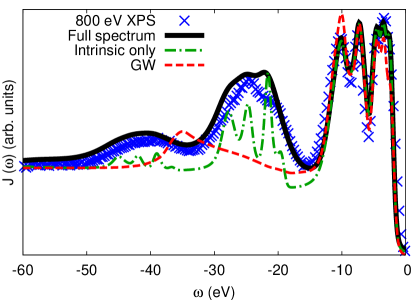
Figure 1: (Color online) Experimental XPS spectrum of Si at 800 eV photon energy (blue crosses), compared to the theoretical intrinsic $A(\omega)$ calculated from $G_{0}W_{0}$ (red dashed), and from Eq. (4) (green dot-dashed). On top of the latter the black solid line also includes extrinsic and interference effects. All spectra contain photoabsorption cross sections, a calculated secondary electron background and 0.4 eV Gaussian broadening to account for finite $k$-point sampling and experimental resolution. The Fermi energy is set to 0 eV.

The experimental data (crosses) are summarized in Fig. 1. One can distinguish the quasiparticle peaks between the Fermi level at zero and the bottom valence at -12 eV, followed by two prominent satellite structures, each at a mutual distance of about 17 eV, as well as a more weakly visible third satellite between -52 and -60 eV. These structures are obviously related to the 17 eV silicon bulk plasmon ISI:A1978FY99000003 .

The exact one-electron Green’s function $\mathcal{G}$ is described by an equation of motion with the form of a functional differential equation kadanoffbaym ,

$$\mathcal{G}=\mathcal{G}_{0}+\mathcal{G}_{0}V_{H}\mathcal{G}+\mathcal{G}_{0}\varphi\mathcal{G}+i\mathcal{G}_{0}v_{c}\frac{\delta\mathcal{G}}{\delta\varphi}.$$ (1)

Here $\mathcal{G}_{0}$ is the non-interacting Green’s function, $\varphi$ is a fictitious external perturbation that is set to zero at the end of the derivation, $v_{c}$ is the bare Coulomb interaction, and all quantities are understood to be matrices in space, spin, and time. The Hartree potential $V_{H}$ gives rise to screening to all orders. Linearizing $V_{H}$ with respect to $\varphi$ yields 2011arXiv1103.1630L

$$\mathcal{G}(t_{1}t_{2})=\mathcal{G}_{H}^{0}(t_{1}t_{2})+\mathcal{G}_{H}^{0}(t_{1}t_{3})\bar{\varphi}(t_{3})\mathcal{G}(t_{3}t_{2})\\ +i\mathcal{G}_{H}^{0}(t_{1}t_{3})\mathcal{W}(t_{3}t_{4})\frac{\delta\mathcal{G}(t_{3}t_{2})}{\delta\bar{\varphi}(t_{4})},$$ (2)

where $\bar{\varphi}$ is equal to $\varphi$ screened by the inverse dielectric function, $\mathcal{W}$ is the screened Coulomb interaction, and $\mathcal{G}_{H}^{0}$ is the Green’s function containing the Hartree potential at vanishing $\bar{\varphi}$; only time arguments are displayed explicitly and repeated indices are integrated. This linearization preserves the main effects of $\mathcal{W}$ and hence of plasmons. With the additional approximation $\frac{\delta\mathcal{G}(t_{3}t_{2})}{\delta\bar{\varphi}(t_{4})}\simeq\mathcal{G}(t_{3}t_{4})\mathcal{G}(t_{4}t_{2})$ one obtains the Dyson equation $\mathcal{G}=\mathcal{G}_{H}^{0}+\mathcal{G}_{H}^{0}\Sigma\mathcal{G}$ in the GWA for the self-energy $\Sigma$. However this approximation can be problematic. For the following analysis we use the standard $G_{0}W_{0}$ approach, where ${\mathcal{G}}_{0}$ is taken from an LDA calculation and ${\mathcal{W}}_{0}$ is the screened interaction in the Random Phase Approximation.

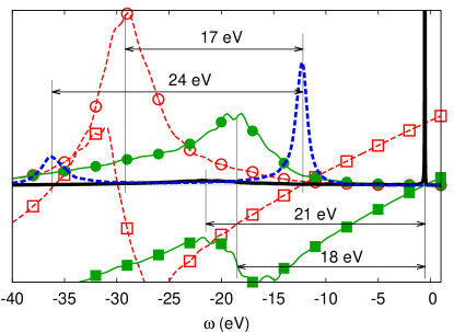
Figure 2: (Color online) $G_{0}W_{0}$ spectral function of bulk silicon for the top and bottom valence bands at the $\Gamma$ point (black solid and blue dashed, respectively). The corresponding imaginary parts of the self-energy (red empty-circles-dashed-line and green full-circles-solid-line) and $\omega-\varepsilon_{H}-\,\mathrm{Re}\Sigma$ (red empty-squares-dashed-line and green full-squares-solid-line) are also shown. The Fermi energy is set to 0 eV.

Fig. 2 shows the $G_{0}W_{0}$ spectral function Fleszar97 $A(\omega)=\frac{1}{\pi}\;{\left|\mathrm{Im}\Sigma(\omega)\right|}/[{\left[\omega-\varepsilon_{H}-\mathrm{Re}\Sigma(\omega)\right]^{2}+\left[\mathrm{Im}\Sigma(\omega)\right]^{2}]}$ of Si at the $\Gamma$ point, for top valence (solid line) and bottom valence (dashed), respectively. The top valence shows a sharp quasiparticle peak followed by a broad, weak satellite structure at about -21 eV. This peak stems from the prominent peak in $\,\mathrm{Im}\,\Sigma$ (full circles) at about $-18$ eV, itself due to the plasmon peak in $\,\mathrm{Im}\mathcal{W}$. It is a typical plasmon satellite, though (cf. Hedin99 ), the QP-satellite spacing is slightly overestimated because the term $\omega-\varepsilon_{H}-\,\mathrm{Re}\Sigma$ (full squares) in the denominator of the expression for $A(\omega)$ is not constant. However the GWA has a more severe problem: for the bottom valence, the satellite structure at about $-36$ eV is much too far from the QP peak at about $-12$ eV, and much too sharp. This satellite does not correspond to a plasmon peak in $\,\mathrm{Im}\Sigma$ (empty circles), but to a zero in $\omega-\varepsilon_{H}-\,\mathrm{Re}\Sigma$ (empty squares) in the denominator of $A(\omega)$, as for a QP peak. It has been interpreted in the HEG as a plasmaron, a coupled hole-plasmon mode Lundqvist1967a ; *ISI:A1968A818100003, but as noted below it is an artifact of the GWA ISI:A1972N855800007 ; ISI:A1973P093700012 . Fig. 1 compares the total $GW$ spectral function (dashed red line) summed over all valence bands and $k$-points, with our XPS data. The effects of cross-sections are included by projecting on angular momenta in atomic spheres using the atomic data of Ref. Yeh85 . The secondary electrons background at energy $\omega$ was determined by integrating the calculated intrinsic spectral intensity between $\omega$ and the Fermi level, similar to PhysRevB.5.4709 . A constant scaling factor was set such that the measured photoemission intensity at the highest binding energy (60 eV), where primary electrons intensity is absent, is reproduced. As expected, the dominant QP spectrum is well described by $GW$, but the satellite is dominated by the plasmaron around $-36$ eV, in complete disagreement with experiment. The experimental plasmon satellite at about $-25$ eV appears only as a weak shoulder in the $GWA$. Thus the plasmaron peak is responsible for the GWA failure ISI:A1972N855800007 ; ISI:A1973P093700012 in silicon.

To go beyond the GW self-energy requires vertex corrections. However, adiabatic vertex corrections (see e.g. PhysRevB.49.8024 ) only lead to renormalization of energies and do not create new structures. Thus alternatively, we concentrate here on dynamical effects, and we choose to approximate directly Eq. (2), without passing through a self-energy. We decouple Eq. (2) approximately by supposing that $\mathcal{G}$ and $\mathcal{G}_{H}$ are diagonal in the same single particle basis. Eq. (2) is then applicable separately for every single matrix element of $\mathcal{G}$ and each state couples independently to the neutral excitations of the system through $\mathcal{W}$ [InasimilarspirittheequationofmotionfortheGreen'sfunctionisdecoupledin:][]Almbladh83. The latter can now be understood as the screened intra-orbital Coulomb matrix element for the chosen state. Such a decoupling approximation can be optimized ISI:A1972N855800007 ; ISI:A1973P093700012 by adding and subtracting a self-energy correction, hence by using a QP Green’s function $\mathcal{G}_{\Delta}$ obtained from a good QP self-energy instead of $\mathcal{G}_{H}$. Since the GWA is currently the state-of-the art for QP properties, we suppose that for every decoupled state $k$, $\mathcal{G}^{k}_{\Delta}(\tau)=i\theta(-\tau)e^{-i\varepsilon_{k}\tau}$ is determined from $\Sigma^{GW}(\varepsilon_{k})$, where $\varepsilon_{k}=\varepsilon^{0}_{k}+\Sigma^{GW}(\varepsilon_{k})$ is the (complex) GW quasiparticle energy and $\tau=t_{1}-t_{2}$. Now Eq. (2) can be solved exactly for each state. Briefly the main steps are: (i) solve the non-interacting ($\mathcal{W}=0$) version of (2), which leads to an explicit solution $\mathcal{G}_{\Delta}^{\varphi}$; (ii) iterate the result $\mathcal{G}=\mathcal{G}_{\Delta}^{\varphi}-\mathcal{G}_{\Delta}^{\varphi}\Delta\mathcal{G}+i\mathcal{G}_{\Delta}^{\varphi}\mathcal{W}\frac{\delta\mathcal{G}}{\delta\bar{\varphi}}$ starting from $\mathcal{G}^{(0)}=\mathcal{G}_{\Delta}^{\varphi}$. Here $\Delta$ compensates for the self-energy insertion used for the optimized decoupling; (iii) use the exact relation $\frac{\delta\mathcal{G}_{\Delta}^{\varphi}(t_{3}t_{2})}{\delta\bar{\varphi}(t_{4})}=\mathcal{G}_{\Delta}^{\varphi}(t_{3}t_{4})\mathcal{G}_{\Delta}^{\varphi}(t_{4}t_{2})=i\mathcal{G}_{\Delta}^{\varphi}(t_{3}t_{2})\theta(t_{2}-t_{4})\theta(t_{4}-t_{1})$ to derive

$$\mathcal{G}(t_{1}t_{2})=\mathcal{G}_{\Delta}(\tau)e^{i\Delta\tau}e^{i\int_{t_{1}}^{t_{2}}dt^{\prime}[\bar{\varphi}(t^{\prime})-\int_{t^{\prime}}^{t_{2}}dt^{\prime\prime}\mathcal{W}(t^{\prime}t^{\prime\prime})]}.$$ (3)

The equilibrium solution is obtained setting $\bar{\varphi}=0$.

In silicon, where the peaks in the loss function are well defined, it is justified to use a single plasmon pole model $\mathcal{W}(\tau)=-i\lambda_{k}\left\{e^{-i\tilde{\omega}_{k}\tau}\theta(\tau)+e^{i\tilde{\omega}_{k}\tau}\theta(-\tau)\right\}$ with plasmon energy $\tilde{\omega}_{k}$ and intrinsic strengths $\lambda_{k}$ for each matrix element of $\mathcal{W}$. Besides $\bar{\varphi}$, the total exponent becomes then $a_{k}\left[e^{i\tilde{\omega}_{k}\tau}-1\right]$ with $a_{k}=\lambda_{k}/\tilde{\omega}_{k}^{2}$ obtained from the corresponding GW results. We find that $a_{k}$ varies around 0.3. Taylor expansion of the exponential leads then to the spectral function

$$A_{k}(\omega)=\frac{e^{-a_{k}}}{\pi}\sum_{n=0}^{\infty}\frac{a_{k}^{n}}{n!}\frac{\Gamma_{k}}{(\omega-\epsilon_{k}+n\,\tilde{\omega}_{k})^{2}+\Gamma_{k}^{2}},$$ (4)

where $\epsilon_{k}=\,\mathrm{Re}[\varepsilon_{k}]$ and $\Gamma_{k}=\,\mathrm{Im}[\varepsilon_{k}]$. Eq. (4) is similar to the plasmon pole version of the CE (cf. Ref. Aryasetiawan96 ). However here the exponential solution arises from a straightforward approximation to the fundamental differential equation (1): the linearization of the Hartree potential reveals the boson of the model (i.e., the plasmon via peaks in $\mathcal{W}$), and the diagonal approximation of $\mathcal{G}$ gives rise to each isolated fermion. Our results are summarized in Fig. 1. The dot-dashed line gives the result of this procedure together with the cross sections and the secondary electron background. The shapes of the QP peaks change little with respect to GW, but now the full series of satellites is present. The internal structure of the satellites which originate from the multiple valence bands, is also reproduced. This validates the decoupling approximation in the dense valence band region where, contrary to the case of an isolated core level, its success is a priori far from obvious. However, the intensity of the observed satellites is significantly underestimated. This discrepancy is similar to that found for the CE in simple metals, where extrinsic losses were suggested as a likely cause Aryasetiawan96 . These might also be reduced by interference effects ISI:A1997WK15700033 . To check this possibility we estimated the contributions from both effects to the satellite strengths $a_{k}$ using Eq. (32) and (36) of Ref. HedinMichielsInglesfield98 . This approach uses a plasmon pole model, Inglesfield fluctuation potentials, and an average over hole positions that takes account of the photoelectron mean free path $\lambda$ HedinMichielsInglesfield98 . We observe that the averaged total satellite line shape in this model is similar to that for the intrinsic part, with a width $\gamma\approx 2$ eV due to plasmon dispersion. Thus we can approximate the extrinsic and interference effects by renormalizing the intrinsic satellite intensity, i.e., by the replacement ${\bar{a}_{k}}=a_{k}+a^{ext}+a^{inf}$ in Eq. (4). These quantities are evaluated with $\omega_{p}=16.7$ eV and $\lambda=17.5$ Å at 800 eV for Si, yielding $a^{ext}$ = 0.63 and $a^{inf}=-.11$. This also modifies the strength $Z_{k}=e^{-{\bar{a}}_{k}}$ of the QP peaks, but preserves overall normalization. The broadening of the satellites must also be increased, $\Gamma\rightarrow\Gamma+n\gamma$. The total spectrum thus obtained (black line) is in unprecedented agreement with experiment. We stress that this result contains no fit parameters besides the two scaling factors (for spectrum and background) due to the arbitrary units of the experiment.

The success of our present approach stresses the need to go beyond the GWA. The exponential representation of $\mathcal{G}$ implicitly corresponds to a vertex correction $\tilde{\Gamma}=-\frac{\delta G^{-1}}{\delta\bar{\varphi}}$ to the self-energy. Since our derivation yields $\mathcal{G}$ as a function of the screened potential $\bar{\varphi}$ (3), this functional derivative can be performed explicitly, using $-\frac{\delta\mathcal{G}^{-1}}{\delta\bar{\varphi}}=\mathcal{G}^{-1}\frac{\delta\mathcal{G}}{\delta\bar{\varphi}}\mathcal{G}^{-1}$. From Eq. (3), a straightforward derivative of $\mathcal{G}$ contains a series of satellite contributions. The two inverse Green’s functions lead to a significant complication, because they contain the inverse of this series. This clearly illustrates the difficulty of modelling $\tilde{\Gamma}$ in order to treat dynamical effects. It suggests rather to concentrate on modelling $\frac{\delta\mathcal{G}}{\delta\bar{\varphi}}$, where the various contributions are simply summed, and hence to search for a self-energy of the form $\Sigma=-i\mathcal{W}\frac{\delta\mathcal{G}}{\delta\bar{\varphi}}\mathcal{G}^{-1}$ instead of $\Sigma=i\mathcal{G}\mathcal{W}\tilde{\Gamma}$. In conclusion, on the basis of our experimental XPS data we have analyzed the failure of GW to reproduce plasmon satellites and linked this failure to the appearance of a artificial plasmaron peak. On the other hand, GW results are fair when the imaginary part of $\Sigma$, hence the intensity of the corresponding plasmon, is small enough so that no sharp plasmaron is created. Thus surprisingly, one might expect GW to work better in describing satellites stemming from local plasmon or interband excitations close to the Fermi level in “strongly correlated” materials than for the strong plasmon structures in conventional semiconductors. Starting from the fundamental equations of MBPT we have derived an exponential solution to the one-particle Green’s function, analogous to that from the CE, that overcomes the drawbacks of the GWA. Comparison to new photoemission data shows that this yields a very good description of the spectral function of bulk silicon, including the satellites series. By calculating the secondary electron background, cross section corrections as well as a correction for extrinsic and interference effects, we achieve an agreement between theory and experiment that can be considered as a benchmark. Our derivation also suggests how the results can be improved in cases where the presently used approximations are inadequate. Finally, by accessing an expression for the vertex function, our approach yields precious hints for directions to take in modeling dynamical effects beyond the GWA.

- (1) F. Aryasetiawan and O. Gunnarsson, Rep. Prog. Phys. 61, 237 (1998)
- (2) W. Aulbur, L. Jonsson, and J. Wilkins, Solid State Physics 54, 1 (2000)
- (3) A. Georges, G. Kotliar, W. Krauth, and M. J. Rozenberg, Rev. Mod. Phys. 68, 13 (1996)
- (4) G. Kotliar et al., Rev. Mod. Phys. 78, 865 (2006)
- (5) F. Offi et al., Phys. Rev. B 76, 085422 (2007)
- (6) L. Hedin, Phys. Scripta 21, 477 (1980)
- (7) L. Hedin, J. Phys.: Cond. Mat. 11, R489 (1999)
- (8) P. Nozières and C. De Dominicis, Phys. Rev. 178, 1097 (1969)
- (9) D. Langreth, Phys. Rev. B 1, 471 (1970)
- (10) F. Bechstedt, “Principles of surface physics,” (Springer, 2003) Chap. 5, pp. 199–201
- (11) L. Hedin, Phys. Rev. 139, A796 (1965)
- (12) L. Hedin and S. Lundqvist, Solid State Physics, Vol. 23 (Academic Press, New York, 1969)
- (13) F. Aryasetiawan, Phys. Rev. B 46, 13051 (1992)
- (14) F. Aryasetiawan, L. Hedin, and K. Karlsson, Phys. Rev. Lett. 77, 2268 (1996)
- (15) M. Vos et al., Phys. Rev. B 66, 155414 (2002)
- (16) A. S. Kheifets et al., Phys. Rev. B 68 (2003)
- (17) B. Holm and F. Aryasetiawan, Phys. Rev. B 56, 12825 (1997)
- (18) M. Vos, A. S. Kheifets, E. Weigold, and F. Aryasetiawan, Phys. Rev. B 63, 033108 (2001)
- (19) F. Polack et al., AIP conf. proc. 1234, 185 (2011)
- (20) N. Bergeard et al., J. Synch. Rad. 18, 245 (2011)
- (21) J. Stiebling, Zeitschrift für Physik B-Condensed Matter 31, 355 (1978)
- (22) L. P. Kadanoff and G. Baym, Quantum Statistical Mechanics (W.A. Benjamin Inc., New York, 1964)
- (23) G. Lani, P. Romaniello, and L. Reining, ArXiv e-prints(2011), arXiv:1103.1630 [cond-mat.str-el]
- (24) A. Fleszar and W. Hanke, Phys. Rev. B 56, 10228 (1997)
- (25) B. Lundqvist, Zeitschrift für Phys. B Cond. Mat. 6, 193 (1967)
- (26) B. Lundqvist, Phys. Kondens. Materie 7, 117 (1968)
- (27) C. Blomberg and B. Bergerse, Can J. Phys. 50, 2286 (1972)
- (28) B. Bergerse, F. Kus, and C. Blomberg, Can J. Phys. 51, 102 (1973)
- (29) J. Yeh and I. Lindau, Atom. Data Nucl. Data Tables 32, 1 (1985)
- (30) D. A. Shirley, Phys. Rev. B 5, 4709 (1972)
- (31) R. Del Sole, L. Reining, and R. W. Godby, Phys. Rev. B 49, 8024 (1994)
- (32) C.-O. Almbladh and L. Hedin, “Handbook on synchrotron radiation,” (North-Holland, Amsterdam, 1983) Chap. 8
- (33) F. Bechstedt, K. Tenelsen, B. Adolph, and R. DelSole, Phys. Rev. Lett. 78, 1528 (1997)
- (34) L. Hedin, J. Michiels, and J. Inglesfield, Phys. Rev. B 58, 15565 (1998)