Kaon and hyperon production in antiproton-induced reactions on nuclei

Abstract

We study the strangeness production in antiproton-nucleus collisions at the beam momenta from 200 MeV/c to 15 GeV/c and in $\bar{p}$ annihilation at rest within the Giessen Botzmann-Uehling-Uhlenbeck (GiBUU) transport model. The GiBUU model contains a very detailed description of underlying antinucleon-nucleon cross sections, in-particular, of the strangeness production channels. We compare our calculations with experimental data on $\Lambda$, $K^{0}_{S}$ and $\bar{\Lambda}$ production in $\bar{p}$A collisions and with earlier intranuclear cascade calculations. The contributions of various partial channels to the hyperon production are reported and systematic differences with the experiment are discussed. The possible formation of bound $\Lambda$- and $\Lambda\Lambda$-nucleus systems is also considered. Finally, results on the $\Xi$ hyperon production are presented in view of forthcoming experiments with antiproton beams at FAIR.

I Introduction

The production of strange particles in antiproton annihilation on nuclei has been a challenge to theory since about two decades when the $\Lambda$ and $K^{0}_{S}$ yields and spectra were measured in the series of bubble chamber experiments Condo et al. (1984); Balestra et al. (1987); Miyano et al. (1988). The most intriguing experimental fact is that the yield ratio $\Lambda/K^{0}_{S}$ is very large $(>2)$ not only for heavy target nuclei ($\bar{p}+^{181}$Ta at 4 GeV/c Miyano et al. (1988)), but even for light ones ($\bar{p}+^{20}$Ne at 608 MeV/c Balestra et al. (1987)). The direct mechanism $\bar{p}p\to\bar{\Lambda}\Lambda$ can only explain less than 20% of the measured $\Lambda$ production cross section for $\bar{p}+^{181}$Ta at 4 GeV/c Ko and Yuan (1987). Thus, the hyperon production in $\bar{p}$ annihilation on nuclei is dominated by the interactions of secondary particles produced in $\bar{p}N$ annihilation with the nuclear medium. Extensive theoretical calculations within the intranuclear cascade (INC) model Cugnon et al. (1990) tend to overestimate the yields of both particle species, $\Lambda$ and $K^{0}_{S}$, and underestimate the yield ratio $\Lambda/K^{0}_{S}$. The latter might indicate the in-medium enhanced cross sections of the strangeness exchange reactions, $\bar{K}N\to Y\pi$ ($Y$ stands for a $\Lambda$- or $\Sigma$-hyperon). The enhanced hyperon production has been also interpreted in terms of $\bar{p}$ annihilations on the clusters of nucleons Cugnon and Vandermeulen (1984); Ko and Yuan (1987) or even the formation of a cold quark-gluon plasma (QGP) Rafelski (1988).

Even more interesting is the double-strange (S=-2) hyperon production in antiproton annihilation on nuclei which has not yet been studied experimentally. The calculations of Ref. Ferro et al. (2007), motivated by the planned Double-Hypernuclei experiment by PANDA@FAIR Pochodzalla (2005); The PANDA Collaboration et al. (2009), take into account only the direct mechanism $\bar{N}N\to\bar{\Xi}\Xi$ which can only account for a few percent of an inclusive $\Xi$ yield. However, the inclusive production of the S=-2 hyperons in $\bar{p}$ annihilation on nuclei is very interesting by itself. This process should be a quite sensitive test for the unusual mechanisms of the $\bar{p}$ annihilation on nuclei, like the QGP formation, since it requires the simultaneous production of two $s\bar{s}$ pairs.

In this work, we study strangeness production in $\bar{p}$-nucleus collisions at $p_{\rm lab}=0.2-15$ GeV/c and in $\bar{p}$-nucleus annihilation at rest within the microscopic GiBUU transport model Buss et al. (2012). We compare our calculations with all available experimental data Condo et al. (1984); Balestra et al. (1987); Miyano et al. (1988); Ahmad et al. (1997) on $\Lambda$, $K_{S}^{0}$ and $\bar{\Lambda}$ production for in-flight annihilation of $\bar{p}$ on nuclei and with earlier calculations within the INC models Cugnon et al. (1990); Strottman and Gibbs (1984); Gibbs and Kruk (1990). We also analyse the selected data set of ref. Riedlberger et al. (1989) on $\pi^{-}$, proton and $\Lambda$ production in $\bar{p}$ annihilation at rest on ¹⁴N. In contrast to the INC models, the GiBUU model includes selfconsistent relativistic mean fields acting on baryons, antibaryons, kaons and antikaons. The selfconsistency means that the mean fields depend on the actual particle densities and currents. This has never been done in the previous transport calculations of antiproton-nucleus reactions. The selfconsistent potential fields are very important, for example, for a realistic treatment of annihilation on light nuclei, when a nucleus get almost destroyed by pions produced in annihilation, and the outgoing particles propagate in much weaker potential fields.

We study in detail the mechanisms of strangeness production by decomposing spectra and reaction rates into the partial contributions from various elementary processes. Estimates for the production probabilities of hypernuclei are also given. Finally, we present the predictions of our model for the $\Xi$ hyperon spectra. We argue that the latter can be used to disentangle the hadronic and hypothetic QGP mechanisms of $\bar{p}$ annihilation on nuclei.

The structure of the paper is as follows. Sec. II contains a brief description of the GiBUU model with an accent on its new and/or improved ingredients, such as, e.g., strangeness production channels in $\bar{N}N$ collisions. In sec. III, we present the results of our calculations for the $\Lambda$, $K^{0}_{S}$ and $\bar{\Lambda}$ production and compare them with experimental data and INC calculations. Then, we give our predictions for the $\Xi$ hyperon production at various $\bar{p}$ beam momenta. Finally, sec. IV summarizes our work.

II Model

The GiBUU model Buss et al. (2012) is a transport-theoretical framework which allows to describe a wide range of photon-, lepton-, hadron-, and nucleus-nucleus reactions. Below we concentrate mostly on the model ingredients which govern strangeness production in antiproton-induced reactions. For other model details relevant for the present study we refer the reader to refs. Buss et al. (2012); Larionov et al. (2008, 2010, 2009); Gaitanos et al. (2010).

The GiBUU model solves the coupled system of kinetic equations for the different hadronic species $i=N,\Delta,Y,Y^{*},\Xi,\pi,K$ etc and respective antiparticles:

$$\frac{1}{p_{0}^{*}}\left[p^{*\mu}\frac{\partial}{\partial x^{\mu}}+\left(p_{\nu}^{*}F_{i}^{\mu\nu}+m_{i}^{*}\frac{\partial m_{i}^{*}}{\partial x_{\mu}}\right)\frac{\partial}{\partial p^{*\mu}}\right]f_{i}(x,{\bf p^{*}})=I_{i}[\{f\}]~{},$$ (1)

where $f_{i}(x,{\bf p^{*}})$ is the phase-space distribution function, $p^{*}=p-V_{i}$ is the kinetic four-momentum, $F_{i}^{\mu\nu}\equiv\partial^{\mu}V_{i}^{\nu}-\partial^{\nu}V_{i}^{\mu}$ is the field tensor, and $m_{i}^{*}=m_{i}+S_{i}$ is the effective mass. The scalar potential $S_{i}=g_{\sigma i}\sigma$ is expressed in terms of the isoscalar $\sigma$ meson ($J^{P}=0^{+}$) field. The vector potential $V_{i}$ includes the contributions from the isoscalar $\omega$ meson ($J^{P}=1^{-}$) field, isovector $\vec{\rho}$ meson ($J^{P}=1^{-}$) field and the electromagnetic field $A$:

$$V_{i}=g_{\omega i}\omega+g_{\rho i}\tau^{3}\rho^{3}+qA~{}.$$ (2)

Here, the isovector term $\propto\rho^{3}$ is included only for nucleons and antinucleons. The collision term $I_{i}[\{f\}]$ in the r.h.s. of Eq. (1) represents the contribution of binary collisions and resonance decays to the partial time derivative $\frac{\partial}{\partial x^{0}}f_{i}(x,{\bf p^{*}})$. The term $\frac{{\bf p^{*}}}{p_{0}^{*}}\nabla f_{i}(x,{\bf p^{*}})$ in the l.h.s. of Eq. (1) is a usual drift term. The term $\propto\frac{\partial}{\partial p^{*\mu}}f_{i}(x,{\bf p^{*}})$ describes the deviation of particle trajectories from straight lines as well as acceleration/deceleration due to the meson mean fields. Without this term, the GiBUU model is basically reduced to a usual cascade model. The meson mean fields $\sigma,\omega,\rho$ and the electromagnetic field $A$ are calculated from the corresponding Lagrange equations of motion neglecting time derivatives Larionov et al. (2008); Gaitanos et al. (2010). This calculation is selconsistent in the sense that the fields are induced by actual particle densities and currents which serve as source terms in the Lagrange equations. The full system of transport equations (1) and meson field equations admits the energy-momentum conservation (c.f. ref. Larionov et al. (2008)).

In order to determine the meson-nucleon coupling constants and the self-interaction parameters of the $\sigma$ field, we use the relativistic mean field (RMF) model in the NL3 version Lalazissis et al. (1997). The coupling constants of mesons with other nonstrange baryonic resonances ($\Delta,N^{*}$ etc) are set equal to the respective meson-nucleon coupling constants. For the meson-hyperon and meson-kaon coupling constants, we apply a simple light quark counting rule by putting

$$\frac{g_{\sigma Y}}{2}=g_{\sigma\Xi}=g_{\sigma K}=\frac{g_{\sigma N}}{3}~{},$$ (3)

$$\frac{g_{\omega Y}}{2}=g_{\omega\Xi}=g_{\omega K}=\frac{g_{\omega N}}{3}~{}.$$ (4)

The coupling constants with the corresponding antiparticles are obtained as follows:

$$\frac{g_{\sigma\bar{B}}}{3\xi}=\frac{g_{\sigma\bar{Y}}}{2}=g_{\sigma\bar{\Xi}}=g_{\sigma\bar{K}}=\frac{g_{\sigma N}}{3}~{},$$ (5)

$$\frac{g_{\omega\bar{B}}}{3\xi}=\frac{g_{\omega\bar{Y}}}{2}=g_{\omega\bar{\Xi}}=g_{\omega\bar{K}}=-\frac{g_{\omega N}}{3}~{},$$ (6)

$$g_{\rho\bar{N}}=\xi g_{\rho N}~{}.$$ (7)

Here, “$B$” denotes any nonstrange baryon, i.e. $B=N,\Delta,N^{*}$ etc. The relative signs in Eqs. (5)-(7) are obtained from the $G$-parities of the meson fields. The factor $\xi=0.22$ is introduced in order to obtain the Schrödinger equivalent potential $U_{\bar{N}}=-150$ MeV for an antiproton at the zero kinetic energy and normal nuclear density $\rho_{0}=0.148$ fm^-3, in agreement with $\bar{p}$-nucleus scattering phenomenology (c.f. Larionov et al. (2009) and refs. therein). One should keep in mind, however, that in experiment only the nuclear surface is tested due to a large annihilation cross section. Thus, an empirical information at $\rho_{0}$ can only be obtained by model dependent extrapolations.

In Table 1, we collect the Schrödinger equivalent potentials of different particles evaluated by using the relations (3)-(7) and the nucleon scalar ($S_{N}=-380$ MeV) and vector ($V_{N}^{0}=308$ MeV) potentials in nuclear matter at $\rho_{0}$ Larionov et al. (2009).

Table 1: The Schrödinger equivalent potentials of different particles at zero kinetic energy,
$U_{i}=S_{i}+V_{i}^{0}+(S_{i}^{2}-(V_{i}^{0})^{2})/2m_{i}$ (in MeV), in nuclear matter at $\rho_{0}$.

$i$	$N$	$\Lambda$	$\Sigma$	$\Xi$	$\bar{N}$	$\bar{\Lambda}$	$\bar{\Sigma}$	$\bar{\Xi}$	$K$	$\bar{K}$
$U_{i}$	-46	-38	-39	-22	-150	-449	-449	-227	-18	-224

The potential depths for nucleon, $\Lambda$ hyperon and antikaon are consistent with phenomenology Friedman and Gal (2007). The $\Sigma$ potential is attractive, which contradicts the analysis of $\Sigma^{-}$ atoms Friedman and Gal (2007). A weak attraction for kaons is also not supported by the analysis of the kaon flow from heavy ion collisions (c.f. Larionov and Mosel (2005) and refs. therein), where a weak repulsion has been found. These drawbacks are the consequences of a simple treatment of particle potentials based on the same RMF model. We do not expect that they sensitively influence our results since the multiplicity of $\Sigma$ hyperons is considerably smaller than the multiplicity of $\Lambda$ hyperons while the kaon potential is weak anyway. The potentials of the $\Xi$ hyperons and antihyperons are still not restricted by any experimental data.

The nucleus is modeled by employing a local density approximation. The momenta of nucleons are sampled uniformly within the spheres of radii

$$p_{F,i}=(3\pi^{2}\rho_{i})^{1/3}~{},~{}~{}~{}i=p,n~{},$$ (8)

by using a Monte Carlo method. The density profiles of protons and neutrons $\rho_{i}(r)$ are obtained from a selfconsistent solution of the relativistic Thomas-Fermi equations Gaitanos et al. (2010). This makes the nucleus stable on the time scale of the order of several 100 fm/c, enough for the most reactions with nuclear targets. The Fermi motion of nucleons results in the smearing of particle production thresholds, which is especially important for the reactions with low-energy projectiles.

For the simulation of an $\bar{p}$-nucleus collision, at $t=0$ an antiproton is placed at the distance 5 fm + nuclear radius from the nuclear center along the collision axis. Such a distant initialization of the antiproton is needed in order to take into account the change of its momentum and trajectory under the action of attractive nuclear and Coulomb potentials Larionov et al. (2009).

For the simulation of annihilation at rest, the initial radial position of the antiproton is chosen according to the probability distribution (c.f. Iljinov et al. (1982); Cugnon and Vandermeulen (1985))

$$dP=C|R_{nl}(r)|^{2}\rho(r)r^{2}dr~{}.$$ (9)

where $R_{nl}(r)$ is the radial wave function of the antiproton in the Coulomb atomic state with quantum numbers $n$ and $l\leq n-1$, $\rho(r)$ is the nucleus density profile, and $C$ is a normalization constant. Quoting ref. Cugnon and Vandermeulen (1985), a cascade of electromagnetic deexcitation of the $\bar{p}$-atom, essentially through the $(n,l=n-1)$ states, emits $X$-rays, which permits us to trace the $\bar{p}$ down to the level where annihilation takes place.

Once a nucleus and an antiproton are initialized, the system of kinetic equations (1) supplemented by the meson field equations is solved by the test particle method in the parallel ensemble mode Bertsch and Das Gupta (1988). Between the two-body collisions, the test particle centroids $({\bf r},{\bf p}^{*})$ propagate according to the Hamiltonian-like equations (c.f. Larionov et al. (2009); Gaitanos et al. (2010)). The two-body collisions are treated in a geometrical picture: the test particles $a$ and $b$ from the same parallel ensemble are allowed to collide if they pass their minimal distance $d_{\rm min}$ during a given time step. Here $d_{\rm min}<\sqrt{\sigma_{\rm tot}^{ab}/\pi}$, where $\sigma_{\rm tot}^{ab}$ is the total interaction cross section depending on the types of colliding particles and invariant energy $\sqrt{s}$. In the present work, we use vacuum cross sections neglecting their possible in-medium modifications. The final state of a two-body collision $ab\to cde...$ is chosen by a Monte Carlo method according to the partial cross sections of various outgoing channels. The final state probability includes the products of Pauli blocking factors $(1-f)$ for the outgoing nucleons. These factors are calculated from the actual time-dependent neutron and proton phase-space distributions. Collisions between the secondary and primary particles as well as between two secondaries are taken into account. The mean fields are recomputed on every time step according to the modified particle densities and currents.

In the case of an antinucleon-nucleon collision, the annihilation may result in a large number of various mesonic final states. This makes the direct parameterization of all partial cross sections practically impossible. Thus, we rely on the statistical annihilation model with SU(3) symmetry Pshenichnov ; Golubeva et al. (1992). This model has been successfully applied in the calculations of pion and proton spectra from $\bar{p}$ annihilation on nuclei at 608 MeV/c within the GiBUU framework Larionov et al. (2009). According to the model Pshenichnov ; Golubeva et al. (1992), the probability of the $\bar{N}N$ annihilation to a given final state meson configuration, which may include up to $n=6$ mesons $\pi,\eta,\omega,\rho,K,\bar{K},K^{*}$ and $\bar{K}^{*}$, is defined as

$$W_{n}(\sqrt{s},I_{1},...,I_{n},Y_{1},...,Y_{n}) = w_{n}(\sqrt{s},I_{1},...,I_{n},Y_{1},...,Y_{n})$$ (10)

$$\times a_{\pi}^{n_{\pi}}a_{\eta}^{n_{\eta}}a_{\omega}^{n_{\omega}}a_{\rho}^{n_{\rho}}a_{K}^{n_{K}+n_{\bar{K}}}a_{K^{*}}^{n_{K^{*}}+n_{\bar{K}^{*}}}~{},$$

where $I_{1},...,I_{n}$ and $Y_{1},...,Y_{n}$ are, respectively, the isospins and hypercharges of outgoing mesons, and $n_{i}$ are the multiplicities of mesons of each type ($i=\pi,\eta,\omega$ etc). The quantity $w_{n}$ is proportional to the phase space volume of a given final state and is calculated assuming that the incoming and outgoing hadrons can be exactly classified according to the SU(3) symmetry. The dimensionless parameters $a_{\pi},a_{\eta},...,a_{K^{*}}$ break the exact SU(3) symmetry. They approximate the unknown parts of matrix elements and depend on the types of the particles and on their internal structure. For the annihilation channels without strangeness, the values $a_{\pi}=1,a_{\eta}=0.13,a_{\omega}=0.18$ and $a_{\rho}=0.24$ were determined in Golubeva et al. (1994) from the best agreement with the data on $\bar{p}p$ annihilation at rest and in flight at $p_{\rm lab}\leq 10$ GeV/c Sedlák and S̆imák (1988). For the parameters related to the strange mesons, we apply the beam momentum dependent expressions obtained from the fit of the $\bar{p}p\to K^{0}_{S}X$ and $\bar{p}n\to K^{-}K^{0}_{S}\pi^{+}\pi^{-}$ cross sections (see Fig. 1 for the $\bar{p}p$ case):

$$a_{K(K^{*})}=0.07\,(0.05)\,C(p_{\text{lab}})~{},$$ (11)

where

$$C(p_{\text{lab}})=\cases{4.2\exp(-1.4p_{\text{lab}})+0.5\exp(-0.16p_{\text{lab}})+1,&for $\bar{p}p$\cr 2.0\exp(-0.7p_{\text{lab}})+0.5\exp(-0.16p_{\text{lab}})+1,&for $\bar{p}n$\cr}$$ (12)

with $p_{\text{lab}}$ being the beam momentum (in GeV/c). The statistical annihilation model works, strictly speaking, only at high beam momenta, when the particle multiplicities are large. At low beam momenta, this model has to be supplemented by the phenomenological branching ratios of the different annihilation channels. For the channels without strange particles, this has been already done in Pshenichnov ; Golubeva et al. (1992). In the present work, we have extended the tables of probabilities for various $\bar{p}p$ and $\bar{p}n$ annihilation channels at rest Pshenichnov ; Golubeva et al. (1992) by including the channels with strange particles $K\bar{K}$, $K^{*}\bar{K}$ + c.c., and $K^{*}\bar{K}^{*}$ (see Appendix A). In order to have a smooth transition from these empirical branching ratios to the description according to the statistical model as the beam energy grows, we determine by a Monte-Carlo method whether the statistical model itself or the empirical branching ratios are used to simulate a given $\bar{N}N$ annihilation event. The probability to choose the tables is

$$P_{\rm at~{}rest}=\max\left(0,1-\frac{\sqrt{s}-2m_{N}}{\sqrt{s_{\rm max}}-2m_{N}}\right)~{},$$ (13)

where $\sqrt{s_{\rm max}}=2.6$ GeV is the maximum invariant energy up to which the annihilation tables at rest still can be selected (respective beam momentum $p_{\rm lab}=2.5$ GeV/c). At the invariant energies above $\sqrt{s_{\rm max}}$, the statistical model is used directly. The momenta of outgoing mesons in an $\bar{N}N$ annihilation event are always sampled microcanonically according to the available phase-space volume, regardless of whether annihilation tables at rest or the statistical model are applied to choose the flavours and charges of the outgoing mesons. This ensures a smooth behavior of the kinematics of produced mesons with increasing beam energy.

Apart from the $\bar{N}N$ annihilation to mesons, we also include elastic (+charge exchange) scattering $\bar{N}N\to\bar{N}N$, $\Delta$ resonance production $\bar{N}N\to\bar{N}\Delta$ (+c.c.), and hyperon production $\bar{N}N\to\bar{\Lambda}\Lambda,~{}\bar{\Sigma}\Lambda(+{\rm c.c}),~{}\bar{\Xi}\Xi$ channels. The corresponding total and angular differential cross section parameterizations are obtained from the fits of empirical data. The cross sections are described in detail in Appendix B.

At $\sqrt{s}>2.37$ GeV, the inelastic production in $\bar{N}N$ collisions is simulated with a help of the Fritiof model Pi (1992). Exception are the processes $\bar{N}N\to\bar{N}N$, $\bar{N}N\to\bar{\Lambda}\Lambda,~{}\bar{\Sigma}\Lambda(+{\rm c.c}),~{}\bar{\Xi}\Xi$ which are either not included or not described well in Fritiof. Thus, we treat these processes separately according to their partial cross sections at any $\sqrt{s}$.

Figure 1: Inclusive cross section of $K_{S}^{0}$ production (upper left panel), the cross section of $K_{S}^{0}$ production in annihilation and nonannihilation channels (lower left and upper right panels, respectively), and the inclusive cross section of the hyperon production (lower right panel) in antiproton-proton collisions as a function of the beam momentum. The experimental data are taken from refs. Ochiai et al. (1984); Baldini et al. (1988).

Figure 1 shows the inclusive cross sections of $K_{S}^{0}$ and hyperon production in $\bar{p}p$ collisions. The partial cross sections of $K_{S}^{0}$ production in the annihilation and nonannihilation events are also shown in the same figure. The experimental data on $K_{S}^{0}$ production are described very well, including the nonannihilation channels, which are simulated by the Fritiof model. The hyperon production cross section is somewhat underestimated at the beam momenta $\sim 4$ GeV/c. This is mainly due to still underestimated cross section of the $\bar{p}p\to\bar{\Lambda}\Lambda X$ inclusive channel above 3 GeV/c, which is practically missed in the Fritiof model. However, we find that, overall, the Fritiof model describes the inelastic production in $\bar{p}p$ collisions better, than, e.g., the Pythia model Sjostrand et al. (2006). Generally, the latter is successfully employed in GiBUU for the description of baryon-baryon and meson-baryon collisions at high invariant energies ($\sqrt{s}>2.6$ GeV and $\sqrt{s}>2.2$ GeV, respectively). We have to only admit one problem. The Pythia model does not include $K^{0}$ and $\bar{K}^{0}$ in its list of the possible incoming particles. Thus, both of them are replaced by $K^{0}_{L}$ in GiBUU every time when Pythia is used. This leads to $\sim 5\%$ violation of the total strangeness conservation in our calculations, which, however, is accurate enough for the present exploratory studies.

The processes of a hyperon scattering, $\Lambda N\to\Lambda N$, $\Lambda N\leftrightarrow\Sigma N$, $\Sigma N\to\Sigma N$, $\Xi N\to\Xi N$, $\Xi N\to\Lambda\Lambda$, $\Xi N\to\Lambda\Sigma$, and of the strangeness exchange on nucleons, $\bar{K}N\to Y\pi$, $\bar{K}N\to\Xi K$, are taken into account in the model. When present, their empirical cross sections have been suitably parameterized or the fits to the existing theoretical calculations have been done Gaitanos et al. (2012); Effenberger (1999). As we will see later on, the strangeness exchange processes are very important for the hyperon production in antiproton-induced reactions on nuclei. In GiBUU, the strangeness exchange reactions $\bar{K}N\to Y\pi$ are partly mediated by the $S=-1$ hyperon resonance formations and decays $\bar{K}N\to Y^{*}\to Y\pi$ Effenberger (1999).

The associated hyperon production is included in GiBUU via reaction channels $\pi N\to YK$, $\eta N\to YK$, $\rho N\to YK$ and $\omega N\to YK$. The cross sections $\pi N\to YK$ have been parameterized according to Ref. Tsushima et al. (1997). The $\eta$-induced associated hyperon production cross sections on proton have been reconstructed from the respective cross sections of the $\pi^{0}$-induced processes at the same invariant energy $\sqrt{s}$ by utilizing the detailed balance relations Cugnon et al. (1989) and isospin invariance:

$$\sigma(\eta p\to K^{+}\Lambda) = \sigma(\pi^{0}p\to K^{+}\Lambda)\frac{p_{\pi N}}{p_{\eta N}}~{},$$ (14)

$$\sigma(\eta p\to K^{+}\Sigma^{0}) = \sigma(\pi^{0}p\to K^{+}\Sigma^{0})\frac{p_{\pi N}}{p_{\eta N}}~{},$$ (15)

$$\sigma(\eta p\to K^{0}\Sigma^{+}) = 2\sigma(\eta p\to K^{+}\Sigma^{0}),~{}$$ (16)

where $p_{\pi N}$ and $p_{\eta N}$ are the center-of-mass (c.m.) momenta for the corresponding initial channels calculated at the same $\sqrt{s}$. Similar formulas have also been used for the $\omega p$ initial channel. For the $\rho$-induced reactions on proton, we have assumed

$$\sigma(\rho p\to K\Lambda) = \sigma(\pi p\to K\Lambda)\frac{p_{\pi N}}{p_{\rho N}}~{},$$ (17)

$$\sigma(\rho p\to K\Sigma) = \sigma(\pi p\to K\Sigma)\frac{p_{\pi N}}{p_{\rho N}}~{},$$ (18)

where the isospin states of all particles match each other. The cross sections of the $\eta$-, $\omega$- and $\rho$-induced reactions on neutron have been obtained by using the isospin reflection from the corresponding cross sections on proton.

We note, finally, that the bubble chamber data on $\Lambda$ production contain also the admixture of $\Lambda$’s produced by the decays $\Sigma^{0}\to\Lambda\gamma$. These decays are not included in GiBUU, since the $\Sigma^{0}$ life time $\tau=7.4\times 10^{-20}~{}{\rm s}\simeq 222000~{}{\rm fm/c}$ is much longer than the typical hadron-nucleus reaction time scale of $\sim 100$ fm/c. Thus, in the present calculations, we simply add the $\Sigma^{0}$ yield to the $\Lambda$ yield.

III Results

III.1 Time evolution of hyperon production

In our calculations, baryons experience the action of attractive mean field potentials. Slow hyperons get captured inside the residual excited nuclear system. This system may evaporate particles and/or decay into fragments, some of which will be single- or double-$\Lambda$ hypernuclei. It is natural to assume that the fragmentation and evaporation will not change much the total yield of hypernuclei; they may, however, affect the production of a given hypernuclear species.

In order to distinguish the hyperons outside and inside the residual nucleus, we have applied a simple criterion based on the relative distance between particles Aichelin (1991): a particle is outside the nucleus if it is separated by the distance larger than some critical distance $d_{c}$ from all other particles of the nucleus. Otherwise, the particle is inside the nucleus. Provided the evolution time is long enough, the result should not be much influenced by the choice of $d_{c}$, if the latter is larger than the internucleon spacing $\sim 1-2$ fm.

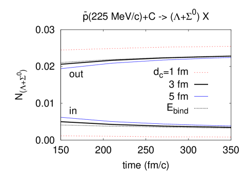
Figure 2: The number of $(\Lambda+\Sigma^{0})$ hyperons outside (out) and inside (in) the residual nucleus per annihilation event as a function of time for $\bar{p}$ annihilations at 225 MeV/c on ¹²C. The calculations are done for three different critical distances $d_{c}$ and for the criterion according to the hyperon binding energy. The results are weighted with the impact parameter of an incoming $\bar{p}$.

This is illustrated in Fig. 2 where we show the number of $(\Lambda+\Sigma^{0})$ hyperons outside and inside the residual nucleus per one annihilation event as a function of time for $\bar{p}$(225 MeV/c)+¹²C collisions for various choices of the critical distance. After $\sim 200$ fm/c the both numbers change very slowly indicating the presence of really captured $\Lambda$ hyperons inside the attractive potential well. For comparison, we also present the results for the bound and unbound hyperons in the same figure. In this case a hyperon $Y$ is considered to be bound (unbound) if $E_{Y}<m_{Y}$ ($E_{Y}>m_{Y}$), where $E_{Y}=\sqrt{({\bf p^{*}})^{2}+(m_{Y}^{*})^{2}}+V_{Y}^{0}$ is its single-particle energy. This criterion allows to identify the captured hyperons somewhat earlier. However, after 200 fm/c it is very close to the criterion according to $d_{c}=3$ fm.

Of course, the capture may only happen if a particle experiences the action of an attractive potential.

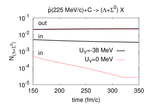
Figure 3: Same as in Fig. 2 but for calculations with and without $\Lambda$-potential at the fixed critical distance $d_{c}=3$ fm.

Fig. 3 compares the time dependence of the number of $\Lambda$’s inside and outside the nucleus for calculations with and without $\Lambda$-potential. As expected, in the calculations without $\Lambda$-potential, the number of hyperons inside the nucleus quickly drops with time indicating that there are no captured $\Lambda$’s in this case.

In the following, we always fix $d_{c}=3$ fm as in ref. Aichelin (1991) and calculate the time evolution until 200 fm/c. Our results for the number of free hyperons, i.e. those outside the residual nucleus, change only by $\sim 10\%$ if we further increase the evolution time (c.f. Fig. 2).

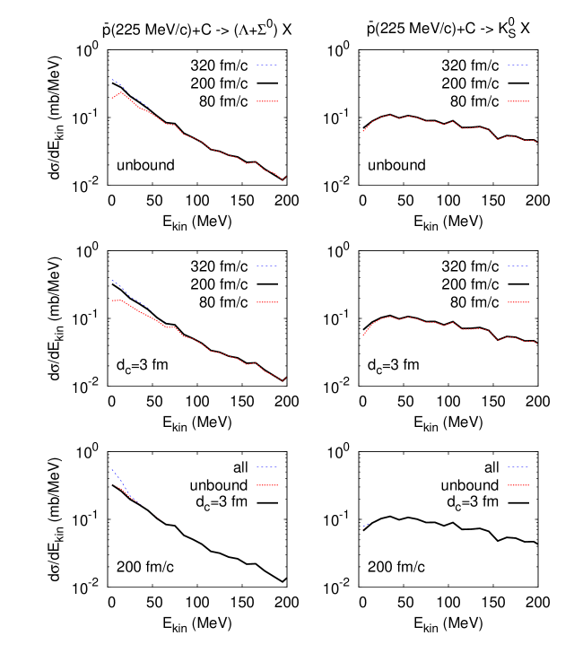
Figure 4: Kinetic energy spectra of $(\Lambda+\Sigma^{0})$ hyperons (left panels) and $K^{0}_{S}$ mesons (right panels). The spectra of free particles selected according to the two different criteria, $E_{i}>m_{i}$ ($i=Y,K$, upper panels) and $d_{c}=3$ fm (middle panels), are plotted at different times. Also the comparison of the spectra obtained with these two criteria with the spectrum of all particles, i.e., without any restrictions is shown at 200 fm/c (lower panels). The number of $K_{S}^{0}$ mesons has been determined from the numbers of $K^{0}$ and $\bar{K}^{0}$ as $N_{K_{S}^{0}}=\frac{1}{2}(N_{K^{0}}+N_{\bar{K}^{0}})$.

As demonstrated in Fig. 4, this change concerns only slow hyperons, while the yields of fast particles are practically stable. In particular, the kaon yields and spectra are not influenced by any further increase of the evolution time.

III.2 Annihilation at rest

We selected the ASTERIX@LEAR data Riedlberger et al. (1989) on charged pion, proton and $\Lambda$ production from $\bar{p}$ annihilation at rest on ¹⁴N. According to ref. Poth et al. (1978), the last observable transition in light antiprotonic atoms is $4\to 3$. Thus we assumed that the antiproton occupies mainly the $n=3,l=2$ level immediately before annihilation which we used as an input in our calculations (see Eq. (9)). We have checked, however, that our results are changed by only few percent if the quantum numbers $n=4,l=3$ are chosen for the antiproton wave function.

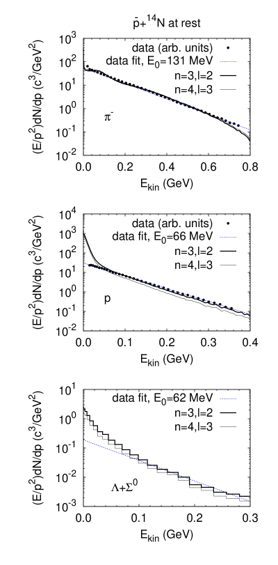
Figure 5: Kinetic energy spectra of negative pions, protons and $(\Lambda+\Sigma^{0})$ hyperons for the $\bar{p}$ annihilation at rest on ¹⁴N. The GiBUU calculations are performed for the n=3, l=2 and n=4, l=3 states of the antiproton. Experimental data and their fits according to the relativistic Maxwell-Boltzmann distribution of Eq. (19) are from ref. Riedlberger et al. (1989). The slope temperatures $E_{0}$ for the experimental spectra are also given on the plots.

Fig. 5 shows the $\pi^{-}$, $p$ and $\Lambda$ kinetic energy spectra in comparison with our calculations. In ref. Riedlberger et al. (1989), the measured spectra were fitted by the relativistic Maxwell-Boltzmann distribution

$$E\frac{dN}{p^{2}dp}=A\exp(-E/E_{0})~{},$$ (19)

with the normalization $A$ and the temperature $E_{0}$ being fit parameters. We observe that the high energy parts of calculated spectra — except for very high energy ($E_{\text{kin}}>0.6$ GeV) pion spectrum — agree with the data and with the Maxwell-Boltzmann formula (19) reasonably well. A slight underprediction of the high-energy pion spectrum can be traced back to the case of $\bar{p}p$ annihilation annihilation at rest (c.f. Fig. B.52 in ref. Buss et al. (2012)). More significant is the deviation from the data at small kinetic energies. We predict the strongly enhanced evaporative emission of the low-energetic particles, in-particular, $p$ and $\Lambda$, in contrast with the ASTERIX data. The enhanced emission of low-energy nucleons is also present in the INC calculations of ref. Cugnon and Vandermeulen (1985) for the $\bar{p}$ annihilations at rest on ⁹⁸Mo.

The calculated pion spectrum also has a clear two-component structure, which seems to be absent in the pion spectra measured by ASTERIX. The high energy pions ($E_{\rm kin}>300$ MeV or $p_{\rm lab}>400$ MeV/c) originate directly from $\bar{N}N$ annihilation almost without rescattering on nucleons. The low energy pions are mostly the products of the $\pi N\to\Delta\to\pi N$ processes. This structure is present in the CALLIOPE@LEAR data McGaughey et al. (1986) for the pion momentum spectra from 608 MeV/c antiproton annihilation on ¹²C and ²³⁸U which agree with the GiBUU calculations very well Larionov et al. (2009).

Although the radial distributions of annihilation points are somewhat different for annihilation at rest and low-energy annihilation in-flight, the angle-integrated momentum spectra of emitted particles are expected to change only a little Cugnon and Vandermeulen (1985). Therefore, we attribute the above discrepancies to the reduced acceptance of the ASTERIX spectrometer for the low-momentum particles, as also mentioned by the authors themselves in ref. Riedlberger et al. (1989).

III.3 Annihilation in-flight

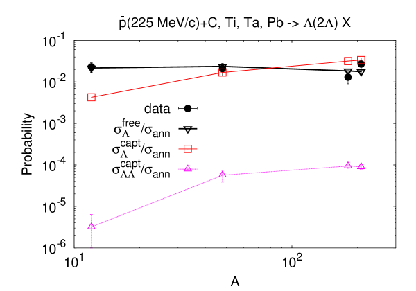
Figure 6: The probability of a free $\Lambda$ as well as one and two captured $\Lambda$’s production per annihilation event vs the target mass number for annihilations of $\bar{p}$ at $p_{\rm lab}=225$ MeV/c on ¹²C,⁴⁸Ti,¹⁸¹Ta and ²⁰⁸Pb. The experimental data for free $\Lambda$ are from Condo et al. (1984).

We start from the lowest beam momenta and consider the reactions $\bar{p}$(0-450 MeV/c)+¹²C,⁴⁸Ti,¹⁸¹Ta and ²⁰⁸Pb measured at BNL Condo et al. (1984). Figure 6 shows the calculated target mass dependence of the free $\Lambda$ production probability per annihilation event together with the data. Note, that the $\bar{p}$-annihilation cross section $\sigma_{\rm ann}\propto A^{2/3}$, i.e., it grows with the target mass number. However, we got rid of this enhancement by dividing out $\sigma_{\rm ann}$ from the $\Lambda$ production cross sections. We also present the calculated production probabilities of nuclear systems with one and two captured $\Lambda$ hyperons in the same reactions. In calculations, the beam momentum was fixed at 225 MeV/c. The free $\Lambda$ production probability is weakly sensitive to the target mass number and agrees with experiment. However, the probabilities of one and two captured $\Lambda$ production grow with the target mass number by almost one order of magnitude from the lightest (¹²C) to the heaviest (²⁰⁸Pb) target. This is expected since, in heavier targets, the produced hyperons are more efficiently decelerated by rescattering on nucleons. The detailed calculations of hyperfragment production in $\bar{p}$ annihilation on nuclei within the coupled GiBUU + statistical multifragmentation models are presented in Ref. Gaitanos et al. (2012).

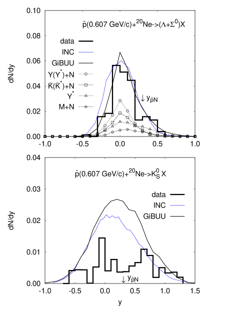
Figure 7: The summed rapidity distributions of $\Lambda$ and $\Sigma^{0}$ hyperons (upper panel) and the rapidity distribution of $K_{S}^{0}$ mesons (lower panel) produced in $\bar{p}$ annihilations on ²⁰Ne at 607 MeV/c — thin solid lines. The integrated distributions give the number of particles per annihilation event. The partial contributions to the hyperon rapidity spectrum (“M” means any nonstrange meson $\pi,\eta,\rho,\omega$) are depicted by lines with open symbols. The INC calculations from ref. Cugnon et al. (1990) are shown by dashed lines. The experimental data (histograms) are taken from ref. Balestra et al. (1987). The c.m. rapidity of an antiproton and a nucleon $y_{\bar{p}N}=0.305$ is shown by arrows.

Figure 7 shows the rapidity distributions of $\Lambda$ hyperons and $K_{S}^{0}$ mesons from $\bar{p}$+²⁰Ne collisions at 608 MeV/c in comparison to the data and to the INC calculations from Cugnon et al. (1990). As we observe, both models agree within $\sim 30\%$. The experimental $\Lambda$ rapidity distribution is rather well described, while the calculated $K_{S}^{0}$ spectra are clearly above the data. Since the direct channel of hyperon production, $\bar{p}p\to\bar{\Lambda}\Lambda$ ($p_{\rm lab}^{\rm thr}=1.439$ GeV/c), is closed at $p_{\rm lab}=608$ MeV/c, the hyperons can only be produced in strangeness exchange processes $\bar{K}(\bar{K}^{*})N\to Y(Y^{*})\pi$, in hyperon resonance formation reactions $\bar{K}N\to Y^{*}$, or in meson-nucleon collisions ($\omega N\to YK$ mostly). Our calculation produces somewhat more $K_{S}^{0}$’s than the INC calculation Cugnon et al. (1990) does. This is partly due to taking into account the target destruction by $\bar{p}$ annihilation in our calculations, which reduces the chances for an $\bar{K}$ to be absorbed. There is also another possible reason for the different results. Both models contain the $\bar{K}N$ elementary cross sections fitted to the experimental data. However, the important difference is that in GiBUU the $Y^{*}$ resonances have finite life times $\sim 1/\Gamma$ and, therefore, can escape out of the nucleus. This effectively reduces the $\bar{K}$ absorption since a $Y^{*}$ excited as the intermediate state of $\bar{K}N$ scattering, $\bar{K}N\to Y^{*}\to\bar{K}N$, “hides” an $\bar{K}$ from interactions with other nucleons.

The $(\Lambda+\Sigma^{0})$ rapidity spectrum shown in Fig. 7 is decomposed to its partial components according to various elementary production channels of $\Lambda$ or $\Sigma^{0}$. We see that the largest contribution is given by the hyperon rescattering on nucleons with flavour and/or charge exchange, in-particular, by the exothermic processes $\Sigma^{+}n\to\Lambda p$ and $\Sigma^{-}p\to\Lambda n$. The main channel of the hyperon production, however, is the strangeness exchange processes $\bar{K}(\bar{K}^{*})N\to Y(Y^{*})\pi$. The rescattering $\Lambda(\Sigma_{0})N\to\Lambda(\Sigma_{0})N$ somewhat distorts the shapes of these partial contributions by shifting the produced $\Lambda$’s($\Sigma^{0}$’s) towards smaller absolute values of rapidity (see also Fig. 9 below).

A more detailed information on the relative importance of various hyperon production channels is given in Table 2.

Table 2: Partial contributions of the different reactions to the multiplicities of $\Lambda$, $\Sigma$ $\bar{K}$ and $K$ per 1000 $\bar{p}$ absorption events on ²⁰Ne at 608 MeV/c. In the calculation of reaction rates we did not distinguish kaons from $K^{*}$’s and antikaons from $\bar{K}^{*}$’s. The negative numbers correspond to the absorption reaction channels for a given particle. Results of the INC calculations Cugnon et al. (1990) are given in brackets.

$\bar{B}B\to\Lambda K$	0 (0)	$\bar{B}B\to\Sigma K$	0 (0)	$\bar{B}B\to\bar{K}X$	57.7 (50.0)	$\bar{B}B\to KX$	57.7 (50.0)
$\pi B\to\Lambda K$	0.6 (1.4)	$\pi B\to\Sigma K$	0.6 (1.0)	$\Sigma M\to\bar{K}X$	0.2	$\phi\to K\bar{K}$	1.9
$\eta B\to\Lambda K$	0.2 (1.5)	$\eta B\to\Sigma K$	0.3 (0.4)	$Y^{*}M\to\bar{K}X$	0.5	$\pi B\to\Lambda K$	0.6 (1.4)
$\rho B\to\Lambda K$	0.9	$\rho B\to\Sigma K$	1.5	$\phi\to K\bar{K}$	1.9	$\eta B\to\Lambda K$	0.2 (1.5)
$\omega B\to\Lambda K$	1.5 (5.0)	$\omega B\to\Sigma K$	3.1 (4.0)	$MM\to K\bar{K}$	3.2	$\rho B\to\Lambda K$	0.9
$\bar{K}B\to\Lambda X$	8.4 (10.0)	$\bar{K}B\to\Sigma X$	10.7 (16.0)	$K\bar{K}\to MM$	-1.2	$\omega B\to\Lambda K$	1.5 (5.0)
$\Sigma B\to\Lambda X$	9.9 (10.0)	$\Sigma B\to\Lambda X$	-9.9 (-10.0)	$\bar{K}B\to\Lambda X$	-8.4 (-10.0)	$\pi B\to\Sigma K$	0.6 (1.0)
$Y^{*}B\to\Lambda X$	1.3	$Y^{*}B\to\Sigma X$	1.4	$\bar{K}B\to\Sigma X$	-10.7 (-16.0)	$\eta B\to\Sigma K$	0.3 (0.4)
$\Lambda B\to\Sigma X$	-0.9 (-0.9)	$\Lambda B\to\Sigma X$	0.9 (0.9)	$\bar{K}B\to Y^{*}$	-17.0	$\rho B\to\Sigma K$	1.5
$\Lambda M\to Y^{*}X$	-1.5	$\Sigma M\to Y^{*}X$	-1.5	$Y^{*}\to\bar{K}N$	6.4	$\omega B\to\Sigma K$	3.1 (4.0)
$Y^{*}\to\Lambda\pi(\eta)$	5.9	$Y^{*}\to\Sigma\pi$	7.6	$\bar{K}B\to Y^{*}\pi$	-2.7	$MM\to K\bar{K}$	3.2
$BB\to\Lambda X$	0.2	$\Sigma M\to\bar{K}X$	-0.2			$K\bar{K}\to MM$	-1.2
						$BB\to KX$	0.3
Sum $\Lambda$	26.5 (27.0)	Sum $\Sigma$	14.5 (12.3)	Sum $\bar{K}$	29.9 (24.0)	Sum $K$	70.6 (63.3)

As one can see by inspecting Table 2, $\sim 80\%$ of the total $Y$ and $Y^{*}$ production rate (without $Y$ and $Y^{*}$ absorption contributions) is caused by the $\bar{K}B\to YX$, $\bar{K}B\to Y^{*}$ and $\bar{K}B\to Y^{*}\pi$ secondary processes. Nevertheless, the associated production $MB\to YK$ constitutes the remaining $20\%$ and, therefore, is quite important as well. In contrast, 80% of the kaon and antikaon production rate is caused by the direct mechanism $\bar{B}B\to K\bar{K}X$. The INC calculation gives larger contributions of the antikaon absorption $\bar{K}B\to YX$ and associated production $MB\to YK$. At the same time, the hyperonic decays of $Y^{*}$ resonances present in GiBUU counterbalance the smaller $\Lambda$ and $\Sigma$ hyperon production by other channels. This leads to rather similar final results for the both models.

It is quite interesting to observe from Table 2 that the $\pi B\to YK$ channels make relatively small contributions to the $\Lambda$ and $\Sigma$ production rates with respect to the $\omega B\to YK$ channels even though there is an abundant pion production in $\bar{p}$ annihilation on nuclei. The reason is that in $\bar{p}$ annihilation at rest or at low $\bar{p}$ beam momentum most of pions are produced with momenta $\sim 0.2-0.4$ GeV/c (c.f. Fig. 2 in ref. Larionov et al. (2009), where the $\pi^{+}$ momentum spectrum is shown for $\bar{p}$+¹²C collisions at 608 MeV/c). This is well below the threshold pion momentum of 0.895 GeV/c for the $\pi N\to\Lambda K$ reaction on a nucleon at rest. On the other hand, an $\omega$ meson is produced in a rather large fraction ($\sim 20\%$) of $\bar{N}N$ annihilation events at rest (c.f. ref. Golubeva et al. (1992)). This favors the exothermic $\omega N\to YK$ reactions, which have a large cross section at low $\omega$ momentum. The situation is, however, different for the energetic $\bar{p}$-nucleus collisions (see Table 3 below).

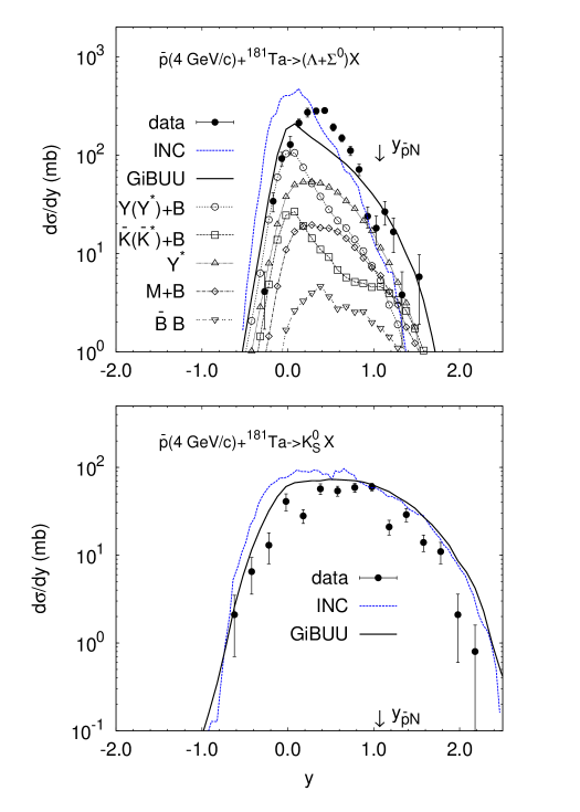
Figure 8: The summed rapidity distributions of $\Lambda$ and $\Sigma^{0}$ (upper panel) and the rapidity distribution of $K^{0}_{S}$ (lower panel) for the collisions $\bar{p}$(4 GeV/c)+¹⁸¹Ta are shown by solid lines. The partial contributions to the hyperon rapidity spectrum (“M” means any nonstrange meson $\pi,\eta,\rho,\omega$, “B” — any nonstrange baryon $N,\Delta,N^{*}$ etc.) are shown by various lines with open symbols. The INC calculations (dashed lines) are taken from ref. Cugnon et al. (1990). The experimental data (solid circles) are from ref. Miyano et al. (1988). The antiproton-nucleon c.m. rapidity $y_{\bar{p}N}=1.078$ is shown by vertical arrows.

At 4 GeV/c, the agreement of our calculations with the experimental $K_{S}^{0}$ spectrum becomes better, as one can see from Fig. 8. However, the ($\Lambda+\Sigma^{0}$) yield is now underpredicted at intermediate rapidities $y\simeq 0.5y_{\bar{p}N}$, where $y_{\bar{p}N}$ is the rapidity of an antiproton-nucleon c.m. system. From the spectrum decomposition into partial channels, which is also given in Fig. 8, we observe qualitatively the same picture as at lower beam momentum 607 MeV/c (Fig. 7 above). Some changes with respect to the lower beam momentum are, however, visible: The hyperon resonance $Y^{*}$ decays grow to the second place in importance. The relative contribution of nonstrange meson-baryon collisions is increased and becomes as important as that of strangeness-exchange reactions. Also a nonnegligible contribution of direct $\bar{B}B$ channels appears now.

The disagreement with the experimental rapidity spectrum of ($\Lambda+\Sigma^{0}$) hyperons at $y\simeq 0.5$ might be due to still underpredicted contribution of the $Y^{*}\to Y\pi$ decays. Indeed, this contribution has a broad maximum at $y\simeq 0.3$, i.e., close to the maximum of the measured rapidity spectrum. Since our calculations tend to overestimate the $K_{S}^{0}$ production, we can assume that the $\bar{K}N\to Y^{*}$ cross sections should be larger. In-particular, the total cross section $K^{-}n\to X$ (or the same cross section of the isospin-reflected channel $\bar{K}^{0}p\to X$) is underestimated at $\sqrt{s}<1.7$ GeV (see Fig. 2.15 in ref. Effenberger (1999)).

Another reason for the deviation with the experimental rapidity spectrum of ($\Lambda+\Sigma^{0}$) hyperons is related to rather uncertain $YN\to YN$ cross sections. Especially the $\Lambda N\to\Lambda N$ cross section is important, as has been noticed, first, by Gibbs and Kruk in ref. Gibbs and Kruk (1990). These authors have applied their INC code Strottman and Gibbs (1984); Gibbs and Kruk (1990) to the reaction $\bar{p}$(4 GeV/c)+¹⁸¹Ta and reproduced the measured $(\Lambda+\Sigma^{0})$ and $K_{S}^{0}$ rapidity spectra very well. They assigned a constant elastic hyperon-nucleon cross section of 14 mb, which is about two times less than the $\Lambda p$ elastic cross section at $p_{\rm lab}\simeq 0.5$ GeV/c (corresponding to the peak position $y\simeq 0.4$ of the measured $\Lambda$ rapidity spectrum, c.f. Fig. 8) in the parameterization of Cugnon et al. Cugnon et al. (1990). Since we have also applied the latter parameterization in the present calculations, this largely explains the shift of our $(\Lambda+\Sigma^{0})$ rapidity spectrum to smaller rapidities with respect to the measured spectrum. Fig. 9 demonstrates the sensitivity of our calculations to the hyperon-nucleon cross sections.

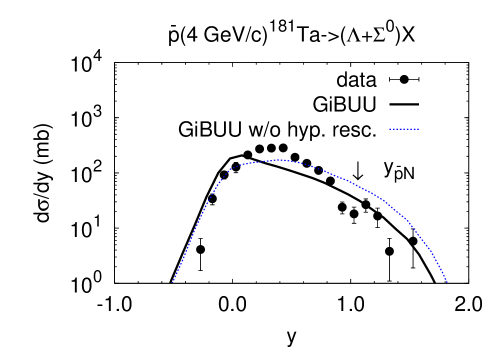
Figure 9: Rapidity distribution of $(\Lambda+\Sigma^{0})$ for antiproton collisions at 4 GeV/c with ¹⁸¹Ta calculated with (solid line) and without (dotted line) taking into account hyperon-nucleon rescattering. Experimental data are from Miyano et al. (1988).

The calculation without hyperon-nucleon rescattering produces the peak position of the calculated $(\Lambda+\Sigma^{0})$ rapidity spectrum close to the experimental one. However, the spectrum at large forward rapidities is now overestimated.

The stopping power of the nuclear medium with respect to the moving hyperon depends not only on the integrated elastic hyperon-nucleon cross section, but also on its angular dependence. For simplicity, we have chosen the hyperon-nucleon cross sections to be isotropic in the c.m. frame. This also contributes to the somewhat too large deceleration of the hyperons. On the other hand, the total yield of ($\Lambda+\Sigma^{0}$) hyperons can be enhanced with increased charge exchange $\Sigma^{-}p\to\Lambda n$ and $\Sigma^{+}n\to\Lambda p$ cross sections which are rather poorly known from experiment.

Detailed information on the various production rates at 4 GeV/c is collected in Table 3.

Table 3: The same as Table 2, but for reaction $\bar{p}$(4 GeV/c)+¹⁸¹Ta.

$\bar{B}B\to\Lambda X$	3.6 (13.0)	$\bar{B}B\to\Sigma X$	2.2 (0)	$\bar{B}B\to\bar{K}X$	109.9 (178.0)	$\bar{B}B\to KX$	110.1 (178.0)
$\pi B\to\Lambda K$	6.6 (30.0)	$\pi B\to\Sigma K$	10.1 (36.0)	$\Sigma M\to\bar{K}X$	1.1	$\phi\to K\bar{K}$	2.8
$\eta B\to\Lambda K$	1.2 (7.0)	$\eta B\to\Sigma K$	2.1 (4.0)	$Y^{*}M\to\bar{K}X$	3.8	$\pi B\to\Lambda K$	6.6 (30.0)
$\rho B\to\Lambda K$	2.5	$\rho B\to\Sigma K$	6.0	$\phi\to K\bar{K}$	2.8	$\eta B\to\Lambda K$	1.2 (7.0)
$\omega B\to\Lambda K$	2.0 (4.0)	$\omega B\to\Sigma K$	7.5 (8.0)	$MM\to K\bar{K}$	32.4	$\rho B\to\Lambda K$	2.5
$\bar{K}B\to\Lambda X$	20.1 (46.0)	$\bar{K}B\to\Sigma X$	13.4 (60.0)	$K\bar{K}\to MM$	-4.5	$\omega B\to\Lambda K$	2.0 (4.0)
$\Sigma B\to\Lambda X$	47.5 (76.0)	$\Sigma B\to\Lambda X$	-47.5 (-76.0)	$\bar{K}B\to\Lambda X$	-20.1 (-46.0)	$\pi B\to\Sigma K$	10.1 (36.0)
$Y^{*}B\to\Lambda X$	11.4	$\Sigma B\to Y^{*}X$	-1.3	$\bar{K}B\to\Sigma X$	-13.4 (-60.0)	$\eta B\to\Sigma K$	2.1 (4.0)
$\Lambda B\to\Sigma X$	-12.5 (-26.0)	$Y^{*}B\to\Sigma X$	15.0	$\bar{K}B\to Y^{*}$	-60.9	$\rho B\to\Sigma K$	6.0
$\Lambda B\to Y^{*}X$	-2.5	$\Lambda B\to\Sigma X$	12.5 (26.0)	$Y^{*}\to\bar{K}N$	22.4	$\omega B\to\Sigma K$	7.5 (8.0)
$\Lambda M\to Y^{*}X$	-10.9	$\Sigma M\to Y^{*}X$	-7.4	$\bar{K}B\to Y^{*}\pi$	-25.0	$MM\to K\bar{K}$	32.4
$Y^{*}\to\Lambda\pi(\eta)$	33.4	$Y^{*}\to\Sigma\pi$	27.2			$K\bar{K}\to MM$	-4.5
$BB\to\Lambda X$	2.4	$\Sigma M\to\bar{K}X$	-1.1			$\bar{Y}B\to KX$	3.8 (11.0)
		$BB\to\Sigma X$	1.2			$BB\to KX$	3.9
Sum $\Lambda$	104.8 (150.0)	Sum $\Sigma$	39.9 (58.0)	Sum $\bar{K}$	48.5 (72.0)	Sum $K$	186.5 (278.0)

One can see from Table 3 that with a relative contribution of $\sim 72\%$ the kaon absorption reactions $\bar{K}B\to YX$, $\bar{K}B\to Y^{*}$ and $\bar{K}B\to Y^{*}\pi$ are still dominating in the total $Y$ and $Y^{*}$ production rate, which is somewhat smaller relative contribution than in the case of $\bar{p}$(607 MeV/c)²⁰Ne. This is expected, since at higher $\bar{p}$ beam momenta more strangeness production channels open. The nonstrange meson-baryon collisions provide the second largest contribution of $\sim 23\%$ to the $Y$ and $Y^{*}$ production rate. The hyperon production in antibaryon-baryon collisions (including direct channel) and in baryon-baryon collisions contributes only $\sim 3\%$ and $2\%$, respectively, to the same rate. On the other hand, as before, in the case of $\bar{p}$(607 MeV/c)²⁰Ne, the antibaryon-baryon collisions dominate in the total $K$($\bar{K}$) production rate contributing $\sim 60\%$. It is interesting, that the meson-meson reactions $MM\to K\bar{K}$ are rather important and contribute $\sim 20\%$ to the $K$ and $\bar{K}$ production rates. This means that the $K\bar{K}$ pair production processes in mesonic cloud created after $\bar{p}$ annihilation should also be taken into account on equal footing with other secondary production channels. Note, however, that in GiBUU the two particles produced in the same two-body collision or resonance decay event are allowed to collide only after at least one of them collided with another particle not involved in this event. This is done in order to avoid multiple chain reactions between the correlated products of the same elementary event, which would otherwise lead to double counting in the production processes and, moreover, violate the molecular chaos assumption.

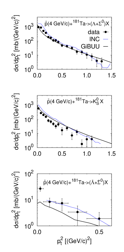
Figure 10: Inclusive transverse momentum spectra of ($\Lambda+\Sigma^{0}$), $K_{S}^{0}$ and ($\bar{\Lambda}+\bar{\Sigma}^{0}$) from collisions $\bar{p}$+¹⁸¹Ta at 4 GeV/c. The INC calculations from Cugnon et al. (1990) are also presented for comparison. The experimental data are taken from ref. Miyano et al. (1988).

Figure 10 shows the inclusive transverse momentum spectra of ($\Lambda+\Sigma^{0}$), $K_{S}^{0}$ and ($\bar{\Lambda}+\bar{\Sigma}^{0}$) from $\bar{p}$(4 GeV/c)+¹⁸¹Ta collisions. The ($\Lambda+\Sigma^{0}$) production at low $p_{t}$ is clearly enhanced due to large cross sections of the exothermic strangeness exchange processes $\bar{K}N\to Y\pi$ induced by slow antikaons. Moreover, the produced hyperons are decelerated by rescattering on nucleons. Our calculations reproduce the shapes of the experimental $p_{t}^{2}$-spectra rather well. There is a remarkable agreement for the absolute values of a ($\Lambda+\Sigma^{0}$) yield at high $p_{t}$. Again, the yield of $K_{S}^{0}$ is somewhat overestimated, while the yield of antihyperons is underestimated by our calculations.

In Table 4 we summarize the results of comparison of our calculations with INC calculations and with experimental data at 0.6 and 4 GeV/c. Both models overestimate the strange quark production and underestimate the ratio $\sigma_{\Lambda+\Sigma^{0}}/\sigma_{K_{S}^{0}}$.

Table 4: The cross sections of the ($\Lambda+\Sigma^{0}$) hyperon, $K_{S}^{0}$ meson and strange quark production (mb) in comparison with the INC results from Cugnon et al. (1990) and experimental data from Balestra et al. (1987); Miyano et al. (1988) for reactions $\bar{p}$(607 MeV/c)+²⁰Ne and $\bar{p}$(4 GeV/c)+¹⁸¹Ta. The “experimental” cross sections of the $s$-quark production are, actually, evaluated in Cugnon et al. (1990) based on some simple relations to the really measured cross sections.

system		$\sigma_{\Lambda+\Sigma^{0}}$	$\sigma_{K_{S}^{0}}$	$\sigma_{\Lambda+\Sigma^{0}}/\sigma_{K_{S}^{0}}$	$\sigma_{s}$
$\bar{p}$+20Ne	GiBUU	18.7	19.2	1.0	50.0
	INC	19.6	13.7	1.4	39.7
	exp	$12.3\pm 2.8$	$5.4\pm 1.1$	$2.3\pm 0.7$	16.9
$\bar{p}$+181Ta	GiBUU	154	121	1.3	387
	INC	275	142	1.9	454
	exp	$193\pm 13$	$82\pm 6$	$2.4\pm 0.3$	$277\pm 21$

To our knowledge, the latest measurement of neutral strange particle production from high-energy antiproton interactions with nuclei was performed at BNL using the Multiparticle Spectrometer (MPS) facility Ahmad et al. (1997). Fig. 11 shows the inclusive cross sections for $\Lambda$, $K_{S}^{0}$, $\bar{\Lambda}$ and strange quark production in collisions of antiprotons at 5, 7 and 9 GeV/c with carbon, copper and lead targets in comparison to the MPS data from Ahmad et al. (1997). Also the INC model Strottman and Gibbs (1984); Gibbs and Kruk (1990) results given in ref. Ahmad et al. (1997) are shown in Fig. 11. The strange quark (or $s\bar{s}$ pair) production cross section has been calculated consistently with ref. Ahmad et al. (1997), i.e. according to the approximate formula

$$\sigma_{s}=\frac{1}{2}(4\sigma_{K_{S}^{0}}+\sigma_{\Lambda}+\sigma_{\Sigma_{0}}+\sigma_{\bar{\Lambda}}+\sigma_{\bar{\Sigma}_{0}})~{},$$ (20)

where $\sigma_{K_{S}^{0}}=(\sigma_{K^{0}}+\sigma_{\bar{K}^{0}})/2$. There is a fair overall agreement of GiBUU calculations with data. In particular, $\Lambda$ and $\bar{\Lambda}$ production on the carbon target is described very well by GiBUU, while for the heavier targets we somewhat underpedict $\Lambda$ and $\bar{\Lambda}$ production. The $K_{S}^{0}$ production cross section on the carbon target is two times overpredicted by GiBUU. On heavier targets, the agreement with experiment on $K_{S}^{0}$ production becomes better, but the slope of the beam momentum dependence of the $K_{S}^{0}$-production cross section seems to be overpredicted. We note, that the data on the inclusive cross sections have been obtained by integration over rapidity region with good acceptance and extrapolated to the $4\pi$ solid angle using the INC calculations. This is partly responsible for a better agreement of the INC results with this experiment. Fig. 12 shows the rapidity distributions of $\Lambda$, $K_{S}^{0}$ and

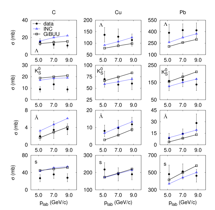
Figure 11: Inclusive cross section of $\Lambda$, $K_{S}^{0}$, $\bar{\Lambda}$ and strange quark (s) production for antiproton interactions at $p_{\text{lab}}=5.2$, 7.0 and 8.8 GeV/c with ¹²C, ⁶⁴Cu and ²⁰⁸Pb targets. The INC calculations and experimental data are from ref. Ahmad et al. (1997).

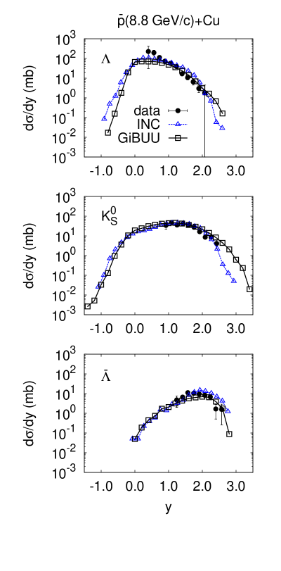
Figure 12: Rapidity distributions of $\Lambda$, $K_{S}^{0}$ and $\bar{\Lambda}$ from $\bar{p}$ interactions with ⁶⁴Cu at 8.8 GeV/c. The INC calculations and experimental data are from ref. Ahmad et al. (1997).

$\bar{\Lambda}$ from antiproton collisions with copper target at 9 GeV/c. As one observes, the GiBUU calculations agree with the data quite well, except the underprediction of $\Lambda$ yield at $y\simeq 0.5$. We also observe a rather close agreement of GiBUU and INC results, which means that the selected observables are, actually, not very sensitive to the model details, once the elementary cross sections are adjusted to the experimental input.

III.4 $S=-2$ hyperon production

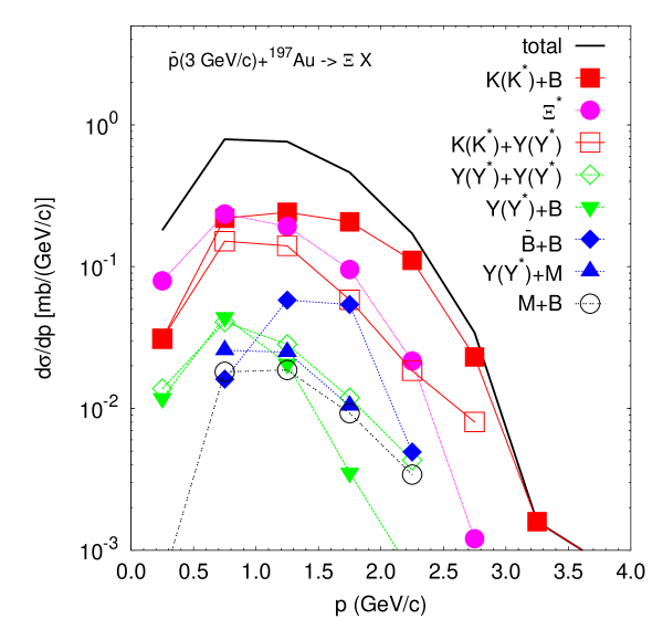
Figure 13: Inclusive momentum spectrum of $\Xi$ hyperons from $\bar{p}$(3 GeV/c)+¹⁹⁷Au collisions (the solid line). The partial contributions according to the parent particles of a $\Xi$ hyperon are depicted by various lines with symbols. In key notations, “M” denotes any nonstrange meson $\pi,\eta,\rho,\omega$, “B” — any nonstrange baryon $N,\Delta,N^{*}$ etc.. The symbol “$K(K^{*})$” denotes both kaon ($K^{*}$) and antikaon ($\bar{K}^{*}$).

Figure 13 shows the inclusive momentum spectrum of $\Xi$ hyperons from $\bar{p}$+¹⁹⁷Au collisions at 3 GeV/c together with the partial contributions from various $\Xi$ production channels. In performing this decomposition, we did not distinguish kaons from antikaons. As one can see from Fig. 13, the (anti)kaon-baryon collisions deliver the main contribution $\sim 35\%$ to the $\Xi$ production, mainly due to the double strangeness exchange channel $\bar{K}N\to K\Xi$. The decays $\Xi^{*}\to\Xi\pi$ — especially important at low transverse momenta of $\Xi$ — make the second largest contribution $\sim 26\%$ to the $\Xi$ production. It is interesting, that the (anti)kaon-hyperon collisions, which are collisions between the secondary particles, contribute also quite appreciably, $\sim 17\%$. Other reaction channels are of relatively minor importance for the inclusive $\Xi$ production. For example, the direct channel $\bar{N}N\to\bar{\Xi}\Xi$ contributes $\sim 6\%$ only; this channel is of primary importance for the planned PANDA experiment on the double-$\Lambda$ hypernuclei production at FAIR Pochodzalla (2005); Ferro et al. (2007).

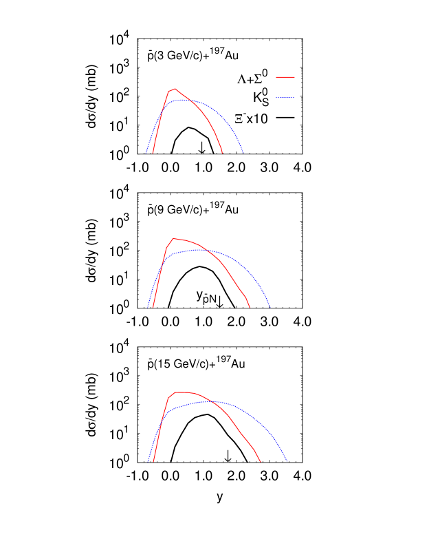
Figure 14: Inclusive rapidity spectra of $\Xi^{-}$, ($\Lambda+\Sigma^{0}$) and $K^{0}_{S}$ from $\bar{p}$+¹⁹⁷Au collisions at 3, 9 and 15 GeV/c. The spectra of $\Xi^{-}$ are multiplied by a factor of 10. The $\bar{p}N$ c.m. rapidity $y_{\bar{p}N}=0.940,~{}1.479$ and $1.733$ for $p_{\rm lab}=3,~{}9$ and $15$ GeV/c, respectively, is shown by vertical arrows.

Figure 14 shows the rapidity spectra of $\Xi^{-}$ hyperons together with the ($\Lambda+\Sigma^{0}$) and $K^{0}_{S}$ rapidity spectra from $\bar{p}$+¹⁹⁷Au collisions at 3, 9 and 15 GeV/c. The $\Xi^{-}$ spectra are about two orders of magnitude below those for the ($\Lambda+\Sigma^{0}$) and $K_{S}^{0}$ production. They are peaked at $y\simeq 0.5,~{}0.9$ and 1.2 for the beam momenta of 3, 9 and 15 GeV/c, respectively. However, the ($\Lambda+\Sigma^{0}$) spectra are always peaked near the target rapidity, $y=0$, even at the largest beam momentum. This is because the hyperon production is dominated by the $\bar{K}N\to Y\pi$ processes with slow antikaons. Moreover, at 3 GeV/c, also the $K^{0}_{S}$ spectrum has a broad maximum at the target rapidity.

The experimental fact that the ($\Lambda+\Sigma^{0}$) and $K^{0}_{S}$ rapidity spectra from $\bar{p}$+¹⁸¹Ta collisions at 4 GeV/c are peaked at nearly the same rapidities (c.f. Fig. 8) has been interpreted by Rafelski Rafelski (1988) as the manifestation of a common production source for strange particles, i.e. of an annihilation fireball with the baryon number $\simeq 10$. The large baryon number is due to absorbing nucleons by the propagating fireball. Rafelski assumed that the fireball undergoes the transition to the supercooled QGP state and then hadronizes. The rapidity spectra of $\Xi$ hyperons would also be peaked at the fireball rapidity if the fireball mechanism would dominate. In our model, a purely hadronic picture emerges instead, where the $\Xi$ production is dominated by the double strangeness exchange processes of $\bar{K}N\to K\Xi$ type. The latter are endothermic and require the momentum of incoming antikaon in the rest frame of a nucleon placed above the threshold value $p_{\rm thr}\simeq 1.05$ GeV/c corresponding to the $\bar{K}N$ c.m. rapidity rapidity of 0.55. This makes the $\Xi$ rapidity spectra shift to higher rapidities. In contrast, the $S=-1$ hyperon production is dominated by the exothermic strangeness exchange $\bar{K}N\to\pi Y$. The cross section of this process grows with decreasing antikaon momentum in the nucleon rest frame. This favors the isotropic production of slow hyperons in the target nucleus rest frame.

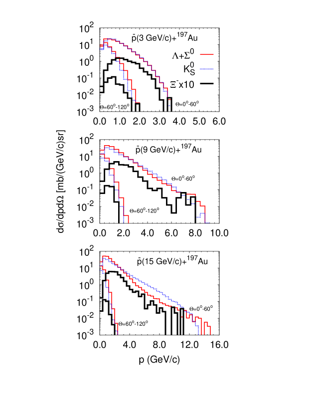
Figure 15: Inclusive laboratory momentum spectra of $\Xi^{-}$, ($\Lambda+\Sigma^{0}$) and $K^{0}_{S}$ from $\bar{p}$(3, 9, 15 GeV/c)+¹⁹⁷Au collisions in the two ranges of the polar angle: $\Theta=0^{o}-60^{o}$ and $\Theta=60^{o}-120^{o}$. The spectra of $\Xi^{-}$ are multiplied by a factor of 10.

Finally, Fig. 15 presents the laboratory momentum spectra of the different strange particles in the forward ($\Theta=0^{o}-60^{o}$) and transverse ($\Theta=60^{o}-120^{o}$) directions for $\bar{p}+^{197}$Au collisions at 3, 9 and 15 GeV/c. The spectra of ($\Lambda+\Sigma^{0}$) hyperons and $K^{0}_{S}$ are rather close to each other both in forward and transverse directions. It is, moreover, interesting that the high-momentum slopes are similar for all considered particles. However, the production of the low-momentum $\Xi^{-}$ hyperons is suppressed due to the dominating $\Xi$ production via the double strangeness exchange in $\bar{K}N\to K\Xi X$ processes.

IV Summary and conclusions

To summarize, we have studied the strange particle production in $\bar{p}$-induced reactions on nuclei by applying the GiBUU model. We have considered both at-rest and in-flight reactions and confronted our results with experimental data Riedlberger et al. (1989); Condo et al. (1984); Balestra et al. (1987); Miyano et al. (1988); Ahmad et al. (1997) on neutral strange particle yields and spectra. We have also compared our calculations with the earlier INC calculations of Cugnon-Deneye-Vandermeulen Cugnon et al. (1990) and Gibbs-Kruk Gibbs and Kruk (1990). Finally, the model predictions for the $\Xi$ hyperon production are given.

So far the main motivation for the experimental studies of strangeness production in antiproton-nucleus reactions has been to find the signatures of QGP production, which can be complementary to similar studies in high-energy heavy-ion collisions. Overall, our results are in a fair agreement with existing experimental data on $K^{0}_{S}$, ($\Lambda+\Sigma^{0}$) and ($\bar{\Lambda}+\bar{\Sigma}^{0}$) production for $\bar{p}$ annihilation on nuclei and with INC models. There seems to be, indeed, no striking disagreements with data on inclusive $\Lambda$, $K_{S}^{0}$ and $\bar{\Lambda}$ production at high beam momenta, which could point to the exotic mechanisms, as it has been already concluded in refs. Gibbs and Kruk (1990); Ahmad et al. (1997).

There are, however, some systematic deviations the origins of which remain to be better understood. The GiBUU and INC models are based on the same hadronic cascade picture but differ in several details like, e.g. the mean field potentials and the treatment of $Y^{*}$ resonances. There is a clear tendency to underestimate the $\Lambda/K^{0}_{S}$ ratio in our calculations. This tendency is present also in the results of INC calculations, although somewhat less pronounced. This problem might be caused by possible in-medium effects on the $\bar{K}N\to YX$ cross section. Poorly known hyperon-nucleon cross sections also strongly influence the observed hyperon spectra. The latter cross sections are also of more general interest, since they are related to the hyperon-nucleon interaction relevant in hypernuclear studies. To disentangle various possibilities, it would be very useful to measure the rapidity spectra of not only neutral strange particles, ($\Lambda+\Sigma^{0}$) and $K_{S}^{0}$, but also of the charged ones, $\Sigma^{\pm}$ and $K^{\pm}$.

The exotic mechanisms of strangeness production may, in-principle, manifest themselves more clearly in the $S=-2$ hyperon production. We have calculated the inclusive production of $\Xi$ hyperons from collisions $\bar{p}$+¹⁹⁷Au at 3-15 GeV/c. The $\Xi^{-}$ rapidity spectra are strongly shifted to forward rapidities in the laboratory system, since the $\Xi$ production via the dominating endothermic $\bar{K}N\to K\Xi$ channel requires a high-momentum initial antikaon. This is in a contrast to the strangeness production mechanism from a moving annihilation fireball proposed by Rafelski Rafelski (1988). Thus a simultaneous measurement of the single- and double-strange hyperon rapidity spectra may serve as a sensitive test for the hadronic and QGP scenarios of strangeness production in $\bar{p}$ annihilation on nuclei. The possibility for such measurements opens up in the planned PANDA experiment at FAIR The PANDA Collaboration et al. (2009).

Appendix A Strangeness production in $\bar{N}N$ annihilation at rest

In this Appendix we list the probabilities for the various channels with strangeness for $\bar{p}p$ and $\bar{p}n$ annihilation at rest (Tables 5 and 6, respectively). We also provide references on source papers. Footnotes explain how some of the probabilities have been obtained from experimental data. Many of the partial probabilities for the $\bar{p}p$ annihilation at rest can be also found in the data compilation Blüm et al. (1988).

Table 5: Probabilities of the different channels with strange mesons for $\bar{p}p$ annihilation at rest (in %).

Channel	Prob.	Ref.	Channel	Prob.	Ref.
$K^{+}K^{-}$ a)	0.091	Amsler et al. (1992); Doser et al. (1988)	$K^{*+}K^{-}\pi^{0}$	0.070	Barash et al. (1966)
$K^{0}\bar{K}^{0}$ a)	0.091	Amsler et al. (1992); Doser et al. (1988)	$K^{*-}K^{+}\pi^{0}$	0.070	Barash et al. (1966)
$K^{+}K^{*-}$	0.071	Soulliere (1987)	$\bar{K}^{*0}K^{0}\pi^{0}$ b)	0.070
$K^{-}K^{*+}$	0.071	Soulliere (1987)	$K^{*0}\bar{K}^{0}\pi^{0}$ b)	0.070
$K^{0}\bar{K}^{*0}$	0.060	Barash et al. (1965)	$K^{*0}K^{-}\pi^{+}$	0.085	Barash et al. (1966)
$\bar{K}^{0}K^{*0}$	0.060	Barash et al. (1965)	$\bar{K}^{*0}K^{+}\pi^{-}$	0.085	Barash et al. (1966)
$K^{*+}K^{*-}$	0.225	Barash et al. (1966)	$K^{0}\bar{K}^{0}\pi^{0}\pi^{0}$ 6)	0.035	Abele et al. (1997); Barash et al. (1966)
$K^{*0}\bar{K}^{*0}$	0.225	Barash et al. (1966)	$K^{+}K^{-}\pi^{0}\pi^{0}$ b)	0.035
$K^{0}\bar{K}^{0}\pi^{0}$ 1)	0.146	Barash et al. (1965)	$K^{0}\bar{K}^{0}\pi^{+}\pi^{-}\pi^{0}$ 7)	0.068	Barash et al. (1967); Reifenröther et al. (1991)
$K^{+}K^{-}\pi^{0}$ b)	0.146		$K^{+}K^{-}\pi^{+}\pi^{-}\pi^{0}$ b)	0.068
$K^{0}K^{-}\pi^{+}$ 2)	0.142	Barash et al. (1965)	$K^{0}K^{-}\pi^{-}\pi^{+}\pi^{+}$ 8)	0.059	Barash et al. (1967)
$\bar{K}^{0}K^{+}\pi^{-}$ 2)	0.142	Barash et al. (1965)	$\bar{K}^{0}K^{+}\pi^{+}\pi^{-}\pi^{-}$ 8)	0.059	Barash et al. (1967)
$K^{0}\bar{K}^{0}\eta$ 3)	0.050	Barash et al. (1967)	$K^{0}K^{-}\pi^{+}\pi^{0}\pi^{0}$ b)	0.042
$K^{+}K^{-}\eta$ b)	0.050		$\bar{K}^{0}K^{+}\pi^{-}\pi^{0}\pi^{0}$ b)	0.042
$K^{0}\bar{K}^{0}\omega$ 3,a)	0.232	Bizzari et al. (1971)	$K^{+}K^{-}\pi^{0}\pi^{0}\pi^{0}$ b)	0.012
$K^{+}K^{-}\omega$ a)	0.232	Bizzari et al. (1971)	$\bar{K}^{0}K^{0}\pi^{0}\pi^{0}\pi^{0}$ b)	0.012
$K^{0}\bar{K}^{0}\rho^{0}$ 4,a)	0.202	Amsler (1986); Heel et al. (1986); Barash et al. (1966); Reifenröther et al. (1991)	$\phi\pi^{+}\pi^{-}$	0.054	Reifenröther et al. (1991)
$K^{+}K^{-}\rho^{0}$ 4,a)	0.202	Amsler (1986); Heel et al. (1986); Barash et al. (1966); Reifenröther et al. (1991)	$\phi\pi^{0}\pi^{0}$ b)	0.011
$K^{0}K^{-}\rho^{+}$ 5)	0.234	Barash et al. (1966)	$\phi\rho^{0}$	0.034	Reifenröther et al. (1991)
$\bar{K}^{0}K^{+}\rho^{-}$ 5)	0.234	Barash et al. (1966)	$\phi\pi^{0}$	0.019	Reifenröther et al. (1991)
$K^{*+}\bar{K}^{0}\pi^{-}$	0.230	Barash et al. (1966)	$\phi\eta$	0.004	Reifenröther et al. (1991)
$K^{*-}K^{0}\pi^{+}$	0.230	Barash et al. (1966)	$\phi\omega$	0.030	Reifenröther et al. (1991)

¹⁾Nonresonance contribution obtained as $B_{K^{0}\bar{K}^{0}\pi^{0}}^{\rm nonres}=B_{K_{S}K_{S}\pi_{0}}+B_{K_{L}K_{L}\pi_{0}}=1.46\cdot 10^{-3}$.

²⁾Nonresonance contributions obtained as

$$B_{K^{0}K^{-}\pi^{+}}^{\rm nonres}=B_{\bar{K}^{0}K^{+}\pi^{-}}^{\rm nonres}=0.5\cdot(B_{K^{0}K^{\pm}\pi^{\mp}}-B_{K^{0}K^{*0},K^{*0}\to K^{\pm}\pi^{\mp}}-B_{K^{\pm}K^{*\mp},K^{*\mp}\to K^{0}\pi^{\mp}})$$

$$=0.5\cdot(4.25-0.85-0.57)\cdot 10^{-3}=1.42\cdot 10^{-3}~{}.$$

³⁾Obtained as $B_{K^{0}\bar{K}^{0}M}=B_{K_{S}K_{S}M}+B_{K_{L}K_{L}M}$, where $M=\eta,~{}\omega$.

⁴⁾Obtained as

$$B_{K^{0}\bar{K}^{0}\rho^{0}}=B_{K^{0}\bar{K}^{0}\pi^{+}\pi^{-}}-B_{K^{*\pm}K^{0}\pi^{\mp},K^{*\pm}\to K^{0}\pi^{\pm}}-B_{K^{*+}K^{*-},K^{*+}\to K^{0}\pi^{+},K^{*-}\to\bar{K}^{0}\pi^{-}}$$

$$-0.34\cdot(B_{\phi\pi^{+}\pi^{-}}+B_{\phi\rho^{0}})=(7.45-3.63-0.57-0.34\cdot(0.54+0.34))\cdot 10^{-3}=2.96\cdot 10^{-3}~{},$$

$$B_{K^{+}K^{-}\rho^{0}}=B_{K^{+}K^{-}\pi^{+}\pi^{-}}-B_{K^{*0}\bar{K}^{*0},K^{*0}\to K^{+}\pi^{-},\bar{K}^{*0}\to K^{-}\pi^{+}}-\frac{2}{3}B_{K^{*0}K^{\pm}\pi^{\mp}}-0.49\cdot(B_{\phi\pi^{+}\pi^{-}}+B_{\phi\rho^{0}})$$

$$=(3.6-1.0-\frac{2}{3}\cdot 1.7-0.49\cdot(0.54+0.34))\cdot 10^{-3}=1.07\cdot 10^{-3}~{}.$$

⁵⁾Obtained as

$$B_{K^{0}K^{\pm}\rho^{\mp}}=B_{K^{0}K^{\pm}\pi^{\mp}\pi^{0}}-B_{K^{*0}K^{\pm}\pi^{\mp},K^{*0}\to K^{0}\pi^{0}}-B_{K^{*\mp}K^{\pm}\pi^{0},K^{*\mp}\to K^{0}\pi^{\mp}}-B_{K^{*\pm}K^{0}\pi^{\mp},K^{*\pm}\to K^{\pm}\pi^{0}}$$

$$-B_{K^{*+}K^{*-},K^{*+}\to K^{0}\pi^{+}(K^{+}\pi^{0}),K^{*-}\to K^{-}\pi^{0}(\bar{K}^{0}\pi^{-})}-B_{K^{*0}\bar{K}^{*0},K^{*0}\to K^{0}\pi^{0}(K^{+}\pi^{-}),\bar{K}^{*0}\to K^{-}\pi^{+}(\bar{K}^{0}\pi^{0})}$$

$$-B_{\bar{K}^{*0}K^{0}\pi^{0},\bar{K}^{*0}\to K^{-}\pi^{+}}-B_{K^{*0}\bar{K}^{0}\pi^{0},K^{*0}\to K^{+}\pi^{-}}$$

$$=(10.38-0.57-0.97-1.04-0.77-1.43-\frac{2}{3}\cdot 1.4)\cdot 10^{-3}=4.67\cdot 10^{-3}~{}.$$

⁶⁾Nonresonance contribution obtained as

$$B_{K^{0}\bar{K}^{0}\pi^{0}\pi^{0}}^{\rm nonres}=B_{K^{0}\bar{K}^{0}\pi^{0}\pi^{0}}-\frac{1}{3}(B_{K^{*0}\bar{K}^{0}\pi^{0}}+B_{\bar{K}^{*0}K^{0}\pi^{0}})-\frac{1}{9}B_{K^{*0}\bar{K}^{*0}}-0.34B_{\phi\pi^{0}\pi^{0}}$$

$$=(1.1-\frac{1}{3}\cdot 1.4-\frac{1}{9}\cdot 2.25-0.34\cdot 0.11)\cdot 10^{-3}=0.35\cdot 10^{-3}~{},$$

assuming that $B_{K^{0}\bar{K}^{0}\pi^{0}\pi^{0}}=B_{K_{L}K_{S}\pi^{0}\pi^{0}}$ according to Abele et al. (1997).

⁷⁾Nonresonance contribution obtained as

$$B_{K^{0}\bar{K}^{0}\pi^{+}\pi^{-}\pi^{0}}^{\rm nonres}=B_{K^{0}\bar{K}^{0}\pi^{+}\pi^{-}\pi^{0}}-0.28\cdot B_{K^{0}\bar{K}^{0}\eta}-0.89\cdot B_{K^{0}\bar{K}^{0}\omega}-0.34\cdot(0.28\cdot B_{\phi\eta}+0.89\cdot B_{\phi\omega})$$

$$=(2.98-0.28\cdot 0.50-0.89\cdot 2.32-0.34\cdot(0.28\cdot 0.036+0.89\cdot 0.30))\cdot 10^{-3}=0.68\cdot 10^{-3}~{}.$$

⁸⁾Obtained as $B_{\bar{K}^{0}K^{+}\pi^{+}\pi^{-}\pi^{-}}=B_{K^{0}K^{-}\pi^{-}\pi^{+}\pi^{+}}=B_{K_{S}K^{\pm}\pi^{\pm}\pi^{\mp}\pi^{\mp}}$.

^a)Averaged with respect to the charged and neutral $K$ or $K^{*}$ production channels.

^b)Obtained by isospin relations from the branching ratio of another channel.

Table 6: Probabilities of the different channels with strange mesons for $\bar{p}n$ annihilation at rest (in %).

Channel	Prob.	Ref.	Channel	Prob.	Ref.
$K^{0}K^{-}$	0.147	Bettini et al. (1969a)	$\bar{K^{*0}}K^{0}\pi^{-}$ 7)	0.130	Bettini et al. (1969a)
$K^{0}K^{*-}$ 1)	0.067	Bettini et al. (1969b)	$K^{*+}K^{-}\pi^{-}$ 8)	0.154	Bettini et al. (1969a)
$K^{-}K^{*0}$ 1)	0.067	Bettini et al. (1969b)	$K^{*-}K^{+}\pi^{-}$ 8)	0.154	Bettini et al. (1969a)
$K^{*-}K^{*0}$ 2)	0.184	Bettini et al. (1969a)	$K^{0}K^{-}\pi^{0}\pi^{0}$ a)	0.043
$K^{0}K^{-}\pi^{0}$ 3)	0.316	Bettini et al. (1969b)	$\bar{K^{0}}K^{+}\pi^{-}\pi^{-}\pi^{0}$	0.016	Bettini et al. (1969a)
$K^{0}\bar{K^{0}}\pi^{-}$ 4)	0.432	Bettini et al. (1969b)	$\bar{K^{0}}K^{0}\pi^{-}\pi^{-}\pi^{+}$	0.075	Bettini et al. (1969a)
$K^{+}K^{-}\pi^{-}$ 5)	0.513	Bettini et al. (1969b)	$K^{-}K^{+}\pi^{-}\pi^{-}\pi^{+}$ a)	0.075
$K^{0}K^{-}\eta$ a)	0.070		$\bar{K^{0}}K^{0}\pi^{0}\pi^{0}\pi^{-}$ a)	0.052
$K^{0}K^{-}\omega$	0.350	Bettini et al. (1969a)	$K^{+}K^{-}\pi^{0}\pi^{0}\pi^{-}$ a)	0.052
$K^{0}K^{-}\rho^{0}$ 6)	0.150	Bettini et al. (1969a)	$K^{0}K^{-}\pi^{+}\pi^{-}\pi^{0}$ 9)	0.025	Bettini et al. (1969a)
$K^{0}\bar{K^{0}}\rho^{-}$ 7)	0.770	Bettini et al. (1969a)	$K^{0}K^{-}\pi^{0}\pi^{0}\pi^{0}$ a)	0.015
$K^{+}K^{-}\rho^{-}$ a)	0.770		$\phi\pi^{-}\pi^{0}$ a)	0.065
$K^{*-}K^{0}\pi^{0}$ 7)	0.245	Bettini et al. (1969a)	$\phi\rho^{-}$ a)	0.068
$K^{*0}K^{-}\pi^{0}$ a)	0.245		$\phi\pi^{-}$	0.088	Bettini et al. (1969b)
$K^{*0}\bar{K^{0}}\pi^{-}$ 7)	0.130	Bettini et al. (1969a)

¹⁾Obtained by averaging the transition rates into $K^{*}\bar{K}+\bar{K^{*}}K$ from ${}^{1}S_{0}~{}I=1$ and ${}^{3}S_{1}~{}I=1$ states as

$$B_{K^{*}\bar{K}+\bar{K^{*}}K}=0.5\cdot(2.0+24.6)\cdot 10^{-4}=13.3\cdot 10^{-4}~{},$$

$$B_{K^{0}K^{*-}}=B_{K^{-}K^{*0}}=0.5\cdot B_{K^{*}\bar{K}+\bar{K^{*}}K}=6.7\cdot 10^{-4}~{}.$$

²⁾Reconstructed from the partial contribution into the $\bar{K^{0}}K^{+}\pi^{-}\pi^{-}$ channel.

³⁾Nonresonance contribution calculated as

$$B_{K^{0}K^{-}\pi^{0}}^{\rm nonres}=B_{K^{0}K^{-}\pi^{0}}-B_{K^{0}K^{*-},K^{*-}\to K^{-}\pi^{0}}-B_{K^{-}K^{*0},K^{*0}\to K^{0}\pi^{0}}$$

$$=B_{K^{0}K^{-}\pi^{0}}-\frac{1}{3}\cdot B_{K^{0}K^{*-}+K^{-}K^{*0}}=(36.0-\frac{1}{3}\cdot 13.3)\cdot 10^{-4}=31.6\cdot 10^{-4}~{}.$$

⁴⁾Nonresonance contribution evaluated as

$$B_{K^{0}\bar{K^{0}}\pi^{-}}^{\rm nonres}=B_{K^{0}\bar{K^{0}}\pi^{-}}-B_{K^{0}K^{*-},K^{*-}\to\bar{K^{0}}\pi^{-}}-B_{\phi\pi^{-},\phi\to K_{L}^{0}K_{S}^{0}}$$

$$=(50.6-\frac{2}{3}\cdot 6.7-0.34\cdot 8.8)\cdot 10^{-4}=43.2\cdot 10^{-4}~{}.$$

⁵⁾Nonresonance contribution evaluated as

$$B_{K^{+}K^{-}\pi^{-}}^{\rm nonres}=B_{K^{+}K^{-}\pi^{-}}-B_{K^{-}K^{*0},K^{*0}\to K^{+}\pi^{-}}-B_{\phi\pi^{-},\phi\to K^{+}K^{-}}$$

$$=(60.0-\frac{2}{3}\cdot 6.7-0.49\cdot 8.8)\cdot 10^{-4}=51.3\cdot 10^{-4}~{}.$$

⁶⁾Reconstructed from the partial contribution to the $K^{0}K^{-}\pi^{-}\pi^{+}$ channel.

⁷⁾Reconstructed from the partial contribution to the $K^{0}_{S}K^{0}_{S}\pi^{-}\pi^{0}$ channel.

⁸⁾Reconstructed from the partial contribution to the $K^{0}K^{-}\pi^{+}\pi^{-}$ and $\bar{K^{0}}K^{+}\pi^{-}\pi^{-}$ channels.

⁹⁾Nonresonance contribution evaluated as

$$B_{K^{0}K^{-}\pi^{+}\pi^{-}\pi^{0}}^{\rm nonres}=B_{K^{0}K^{-}\pi^{+}\pi^{-}\pi^{0}}-B_{K^{0}K^{-}\omega,\omega\to\pi^{+}\pi^{-}\pi^{0}}$$

$$=(33.6-0.89\cdot 35.0)\cdot 10^{-4}=2.5\cdot 10^{-4}~{}.$$

^a)Obtained by isospin relations from the branching ratio of another channel.

Appendix B Elementary cross sections

In this Appendix we describe the cross sections of the hyperon production in $\bar{N}N$ collisions. Other partial cross sections of the $\bar{N}N$ collisions are described in Appendix B.2 of ref. Buss et al. (2012).

The $\bar{p}p\to\bar{\Lambda}\Lambda$ and $\bar{p}p\to\bar{\Lambda}\Sigma^{0}+(\mbox{c.c.})$ cross sections (in mb) are parameterized as a function of the invariant energy $\sqrt{s}$ (in GeV) by the following expressions:

$$\sigma_{\bar{p}p\to\bar{\Lambda}\Lambda}=\cases{0,&$\sqrt{s}<2.232$\cr 0.0357(\sqrt{s}-2.232)^{0.5}+9.005(\sqrt{s}-2.232)^{1.5},&$2.232<\sqrt{s}<2.252$\cr\mbox{max}(0.01,0.726(s/4.982-1)^{0.774}(4.982/s)^{3.350}),&$2.252<\sqrt{s}$}$$ (21)

$$\sigma_{\bar{p}p\to\bar{\Lambda}\Sigma^{0}+\mbox{c.c.}}=\cases{0~{},&~{}~{}~{}$\sqrt{s}<2.308$\cr 0.184(s/5.327-1)^{0.437}(5.327/s)^{1.850}~{},&~{}~{}~{}$2.308<\sqrt{s}$~{}.}$$ (22)

The functional form in (21) at lower energies is adopted from ref. Barnes et al. (1989), however, with slightly different numerical parameters. The parameterization used in (21) at higher energies and in (22) is taken from ref. Tsushima et al. (1999). The numerical parameters in (21) and (22) are obtained by the fit to the world data on the cross sections $\bar{p}p\to\bar{\Lambda}\Lambda$ and $\bar{p}p\to\bar{\Lambda}\Sigma^{0}+\mbox{c.c.}$ from Baldini et al. (1988).

For the $\bar{p}p\to\bar{\Xi}^{+}\Xi^{-}$ cross section only the value of $2$ $\mu$b at 3 GeV/c is known experimentally Baldini et al. (1988). Thus, we simply assume the constant cross section above threshold:

$$\sigma_{\bar{p}p\to\bar{\Xi}^{+}\Xi^{-}}=\sigma_{\bar{p}p\to\bar{\Xi}^{0}\Xi^{0}}=\cases{0~{}\mu\mbox{b},&$\sqrt{s}<2.630$ GeV\cr 2~{}\mu\mbox{b},&$2.630$ GeV $<\sqrt{s}$~{}.}$$ (23)

The cross sections involving $n,~{}\bar{n},~{}\Delta$ and $\bar{\Delta}$ in the initial state are obtained from the isospin relations as

$$\sigma_{\bar{n}n\to\bar{\Lambda}\Lambda} = \sigma_{\bar{p}p\to\bar{\Lambda}\Lambda}~{},$$ (24)

$$\sigma_{\bar{B}B\to\bar{\Lambda}\Sigma+\mbox{c.c.}} = 2\sigma_{0}\left\langle I^{\bar{B}}\,I_{z}^{\bar{B}};I^{B}\,I_{z}^{B}|1\,I_{z}^{\Sigma}\right\rangle^{2}~{},$$ (25)

$$\sigma_{\bar{B}B\to\bar{\Xi}\Xi} = \sigma_{1}\sum_{I=0,1}\,\left\langle I^{\bar{B}}\,I_{z}^{\bar{B}};I^{B}\,I_{z}^{B}|I\,(I_{z}^{\bar{B}}+I_{z}^{B})\right\rangle^{2}\left\langle\frac{1}{2}\,I_{z}^{\bar{\Xi}};\frac{1}{2}\,I_{z}^{\Xi}|I\,(I_{z}^{\bar{B}}+I_{z}^{B})\right\rangle^{2}$$ (26)

where $\sigma_{0}=\sigma_{\bar{p}p\to\bar{\Lambda}\Sigma^{0}+\mbox{c.c.}}$, $\sigma_{1}=2\sigma_{\bar{p}p\to\bar{\Xi}^{+}\Xi^{-}}$, $B$ stands for $N$ or $\Delta$, and only the combinations $\bar{N}N$, $\bar{\Delta}N$ and $\bar{N}\Delta$ of incoming particles are taken into account. Equations (25) and (26) can be simplified, which gives the following:

$$\sigma_{\bar{n}n\to\bar{\Lambda}\Sigma^{0}+\mbox{c.c.}} = \sigma_{0}~{},$$ (27)

$$\sigma_{\bar{p}n\to\bar{\Lambda}\Sigma^{-}+\Lambda\bar{\Sigma}^{-}} = 2\sigma_{0}~{},$$ (28)

$$\sigma_{\bar{\Delta}^{-}p\to\bar{\Lambda}\Sigma^{0}+\mbox{c.c.}}=\sigma_{\bar{\Delta}^{0}n\to\bar{\Lambda}\Sigma^{0}+\mbox{c.c.}} = \sigma_{0}~{},$$ (29)

$$\sigma_{\bar{\Delta}^{-}n\to\bar{\Lambda}\Sigma^{-}+\Lambda\bar{\Sigma}^{-}}=\sigma_{\bar{\Delta}^{0}p\to\bar{\Lambda}\Sigma^{+}+\Lambda\bar{\Sigma}^{+}} = \frac{1}{2}\sigma_{0}~{},$$ (30)

$$\sigma_{\bar{\Delta}^{--}p\to\bar{\Lambda}\Sigma^{-}+\Lambda\bar{\Sigma}^{-}}=\sigma_{\bar{\Delta}^{+}n\to\Lambda\bar{\Sigma}^{+}+\bar{\Lambda}\Sigma^{+}} = \frac{3}{2}\sigma_{0}~{}$$ (31)

$$\sigma_{\bar{n}n\to\Xi^{-}\bar{\Xi}^{+}+\Xi^{0}\bar{\Xi}^{0}}=\sigma_{\bar{p}n\to\Xi^{-}\bar{\Xi}^{0}} = \sigma_{1}~{},$$ (32)

$$\sigma_{\bar{\Delta}^{-}p\to\Xi^{-}\bar{\Xi}^{+}+\Xi^{0}\bar{\Xi}^{0}}=\sigma_{\bar{\Delta}^{0}n\to\Xi^{-}\bar{\Xi}^{+}+\Xi^{0}\bar{\Xi}^{0}} = \frac{1}{2}\sigma_{1}~{},$$ (33)

$$\sigma_{\bar{\Delta}^{-}n\to\Xi^{-}\bar{\Xi}^{0}}=\sigma_{\bar{\Delta}^{0}p\to\Xi^{0}\bar{\Xi}^{+}} = \frac{1}{4}\sigma_{1}~{},$$ (34)

$$\sigma_{\bar{\Delta}^{--}p\to\Xi^{-}\bar{\Xi}^{0}}=\sigma_{\bar{\Delta}^{+}n\to\Xi^{0}\bar{\Xi}^{+}} = \frac{3}{4}\sigma_{1}$$ (35)

The partial cross sections for the different outgoing channels shown with a “+” sign in (27) - (33) are equal to each other. The expressions for the charged conjugated reaction channels are obtained by replacing all particles by the corresponding antiparticles.

The angular differential cross sections for the $\bar{N}N\to\bar{\Lambda}\Lambda$ process at $\sqrt{s}>2.37$ GeV ($p_{\rm lab}>1.830$ GeV/c) and for $\bar{N}N\to\bar{\Lambda}\Sigma,\Lambda\bar{\Sigma}$ processes are chosen according to the phenomenological Regge-like fit of ref. Sadoulet (1969). At $\sqrt{s}<2.37$ GeV, we fitted the experimental angular distributions for the $\bar{N}N\to\bar{\Lambda}\Lambda$ scattering of refs. Barnes et al. (1987, 1989, 1991, 1996); Jayet et al. (1978) by the following expression:

$$\frac{d\sigma_{\bar{N}N\to\bar{\Lambda}\Lambda}}{dt}=[a_{0}+a_{1}\exp(a_{2}(t_{\rm min}-t))]~{}\mu\mbox{b/GeV}^{2}~{},$$ (36)

where $t_{\rm min}=-(p_{\bar{N}N}-p_{\bar{\Lambda}\Lambda})^{2}$ (in GeV²),

$$a_{0} = (19.1946+132202\epsilon^{2.5})/(1+42592\epsilon^{3.5})~{},$$ (37)

$$a_{1} = (277.044\epsilon^{0.25}-3145.39\epsilon+4993140\epsilon^{2.8})/(1+19075.7\epsilon^{3})~{},$$ (38)

$$a_{2} = \cases{67357.8\epsilon-257.692,&$\epsilon\leq 0.0033$\cr 4.66944\ln(1.49962\epsilon),&$0.0033<\epsilon$~{}.}$$ (39)

where $\epsilon=\sqrt{s}-2m_{\Lambda}$ (in GeV). For the $\bar{B}B\to\bar{Y}Y$ processes involving $\Delta$ or $\bar{\Delta}$ in the initial state and for the $\bar{B}B\to\bar{\Xi}\Xi$ processes we assume the isotropic angular differential cross sections in the c.m. frame.

References

- Condo et al. (1984) G. T. Condo, T. Handler, and H. O. Cohn, Phys. Rev. C29, 1531 (1984).
- Balestra et al. (1987) F. Balestra et al., Phys. Lett. B194, 192 (1987).
- Miyano et al. (1988) K. Miyano et al., Phys. Rev. C38, 2788 (1988).
- Ko and Yuan (1987) C. M. Ko and R. Yuan, Phys. Lett. B192, 31 (1987).
- Cugnon et al. (1990) J. Cugnon, P. Deneye, and J. Vandermeulen, Phys. Rev. C41, 1701 (1990).
- Cugnon and Vandermeulen (1984) J. Cugnon and J. Vandermeulen, Phys. Lett. B146, 16 (1984).
- Rafelski (1988) J. Rafelski, Phys. Lett. B207, 371 (1988).
- Ferro et al. (2007) F. Ferro, M. Agnello, F. Iazzi, and K. Szymańska, Nucl. Phys. A789, 209 (2007).
- Pochodzalla (2005) J. Pochodzalla, Nucl. Phys. A754, 430 (2005).
- The PANDA Collaboration et al. (2009) The PANDA Collaboration, M. F. M. Lutz, B. Pire, O. Scholten, and R. Timmermans, arXiv:0903.3905 (2009).
- Buss et al. (2012) O. Buss et al., arXiv:1106.1344, Phys. Rept. in press (2012).
- Ahmad et al. (1997) S. Ahmad, B. Bonner, J. Buchanan, P. Carter, C. Chan, et al., Nucl.Phys.Proc.Suppl. 56A, 118 (1997).
- Strottman and Gibbs (1984) D. Strottman and W. Gibbs, Phys.Lett. B149, 288 (1984).
- Gibbs and Kruk (1990) W. Gibbs and J. Kruk, Phys.Lett. B237, 317 (1990).
- Riedlberger et al. (1989) J. Riedlberger et al., Phys. Rev. C40, 2717 (1989).
- Larionov et al. (2008) A. B. Larionov, I. N. Mishustin, L. M. Satarov, and W. Greiner, Phys. Rev. C78, 014604 (2008).
- Larionov et al. (2010) A. B. Larionov, I. N. Mishustin, L. M. Satarov, and W. Greiner, Phys. Rev. C82, 024602 (2010), eprint 0912.1794.
- Larionov et al. (2009) A. B. Larionov, I. A. Pshenichnov, I. N. Mishustin, and W. Greiner, Phys. Rev. C80, 021601 (2009).
- Gaitanos et al. (2010) T. Gaitanos, A. B. Larionov, H. Lenske, and U. Mosel, Phys. Rev. C81, 054316 (2010), eprint 1003.4863.
- Lalazissis et al. (1997) G. A. Lalazissis, J. König, and P. Ring, Phys. Rev. C55, 540 (1997).
- Friedman and Gal (2007) E. Friedman and A. Gal, Phys. Rept. 452, 89 (2007).
- Larionov and Mosel (2005) A. B. Larionov and U. Mosel, Phys. Rev. C72, 014901 (2005).
- Iljinov et al. (1982) A. S. Iljinov, V. I. Nazaruk, and S. E. Chigrinov, Nucl. Phys. A382, 378 (1982).
- Cugnon and Vandermeulen (1985) J. Cugnon and J. Vandermeulen, Nucl. Phys. A445, 717 (1985).
- Bertsch and Das Gupta (1988) G. F. Bertsch and S. Das Gupta, Phys. Rept. 160, 189 (1988).
- (26) I. A. Pshenichnov, doctoral thesis, INR, Moscow, 1998.
- Golubeva et al. (1992) E. S. Golubeva, A. S. Iljinov, B. V. Krippa, and I. A. Pshenichnov, Nucl. Phys. A537, 393 (1992).
- Golubeva et al. (1994) E. S. Golubeva, A. S. Iljinov, and I. A. Pshenichnov, Phys. Atom. Nucl. 57, 1672 (1994).
- Sedlák and S̆imák (1988) J. Sedlák and V. S̆imák, Fiz. Elem. Chast. Atom. Yadra 19, 445 (1988).
- Pi (1992) H. Pi, Comput. Phys. Commun. 71, 173 (1992).
- Ochiai et al. (1984) F. Ochiai et al., Z. Phys. C23, 369 (1984).
- Baldini et al. (1988) A. Baldini, V. Flaminio, W. G. Moorhead, D. R. O. Morrison, and H. Schopper, Landolt-Börnstein, New Series, Springer Verlag Berlin, Germany 1/12B (1988).
- Sjostrand et al. (2006) T. Sjostrand, S. Mrenna, and P. Skands, JHEP 05, 026 (2006), eprint hep-ph/0603175.
- Gaitanos et al. (2012) T. Gaitanos, A. B. Larionov, H. Lenske, and U. Mosel, arXiv:1111.5748, Nucl. Phys. A in press (2012).
- Effenberger (1999) M. Effenberger, Ph.D. thesis, Justus-Liebig-Universität Gießen (1999), available online at http://theorie.physik.uni-giessen.de/.
- Tsushima et al. (1997) K. Tsushima, S. W. Huang, and A. Faessler, Austral. J. Phys. 50, 35 (1997), eprint nucl-th/9602005.
- Cugnon et al. (1989) J. Cugnon, P. Deneye, and J. Vandermeulen, Phys. Rev. C40, 1822 (1989).
- Aichelin (1991) J. Aichelin, Phys. Rept. 202, 233 (1991).
- Poth et al. (1978) H. Poth et al., Nucl. Phys. A294, 435 (1978).
- McGaughey et al. (1986) P. L. McGaughey et al., Phys. Rev. Lett. 56, 2156 (1986).
- Blüm et al. (1988) P. Blüm, G. Büche, and H. Koch, Kernforschungszentrum Karlsruhe, Primärbericht 14.02.01P29A (1988).
- Amsler et al. (1992) C. Amsler et al. (Crystal Barrel), Phys. Lett. B297, 214 (1992).
- Doser et al. (1988) M. Doser et al. (ASTERIX), Phys. Lett. B215, 792 (1988).
- Barash et al. (1966) N. Barash, L. Kirsch, D. Miller, and T. H. Tan, Phys. Rev. 145, 1095 (1966).
- Soulliere (1987) M. J. Soulliere (LEAR PS183) (1987), uMI-87-14884.
- Barash et al. (1965) N. Barash et al., Phys. Rev. 139, B1659 (1965).
- Abele et al. (1997) A. Abele et al. (Crystal Barrel), Phys. Lett. B415, 280 (1997).
- Barash et al. (1967) N. Barash, L. Kirsch, D. Miller, and T. H. Tan, Phys. Rev. 156, 1399 (1967).
- Reifenröther et al. (1991) J. Reifenröther et al. (ASTERIX), Phys. Lett. B267, 299 (1991).
- Bizzari et al. (1971) R. Bizzari, L. Montanet, S. Nilsson, C. D’ Andlau, and J. Cohen-Ganouna, Nucl. Phys. B27, 140 (1971).
- Amsler (1986) C. Amsler (1986), rapporteur’s talk given at the 8th European Symposium on Nucleon-Antinucleon Interactions, Thessaloniki, Greece, Sep 1-5, 1986, eprint CERN/EP-86-178.
- Heel et al. (1986) M. Heel et al. (1986), proceedings of the 8th European Symposium on Nucleon-Antinucleon Interactions, Thessaloniki, Greece, Sep 1-5, 1986, pp. 55-70.
- Bettini et al. (1969a) A. Bettini et al., Nuovo Cim. A62, 1038 (1969a).
- Bettini et al. (1969b) A. Bettini et al., Nuovo Cim. A63, 1199 (1969b).
- Barnes et al. (1989) P. D. Barnes et al., Phys. Lett. B229, 432 (1989).
- Tsushima et al. (1999) K. Tsushima, A. Sibirtsev, and A. W. Thomas, Phys. Rev. C59, 369 (1999).
- Sadoulet (1969) B. Sadoulet (1969), eprint CERN-HERA-69-2.
- Barnes et al. (1987) P. D. Barnes et al., Phys. Lett. B189, 249 (1987).
- Barnes et al. (1991) P. D. Barnes et al., Nucl. Phys. A526, 575 (1991).
- Barnes et al. (1996) P. D. Barnes et al., Phys. Rev. C54, 2831 (1996).
- Jayet et al. (1978) B. Jayet et al., Nuovo Cim. A45, 371 (1978).