Computing fluxes and chemical potential distributions in biochemical networks: energy balance analysis of the human red blood cell

Abstract

The analysis of non-equilibrium steady states of biochemical reaction networks relies on finding the configurations of fluxes and chemical potentials satisfying stoichiometric (mass balance) and thermodynamic (energy balance) constraints. Efficient methods to explore such states are crucial to predict reaction directionality, calculate physiologic ranges of variability, estimate correlations, and reconstruct the overall energy balance of the network from the underlying molecular processes. While different techniques for sampling the space generated by mass balance constraints are currently available, thermodynamics is generically harder to incorporate. Here we introduce a method to sample the free energy landscape of a reaction network at steady state. In its most general form, it allows to calculate distributions of fluxes and concentrations starting from trial functions that may contain prior biochemical information. We apply our method to the human red blood cell’s metabolic network, whose space of mass-balanced flux states has been sampled extensively in recent years. Specifically, we profile its thermodynamically feasible flux configurations, characterizing in detail how fluctuations of fluxes and potentials are correlated. Based on this, we derive the cell’s energy balance in terms of entropy production, chemical work done and thermodynamic efficiency.

I Introduction

The dynamics of a chemical reaction network is ruled by the underlying thermal fluctuations through the Arrhenius law that relates the rates of reactions to the activation energies and the strength of noise (the temperature). When non-equilibrium steady states (NESS) are reached, the net flow of reactions is constrained to proceed downhill in the free energy landscape [1, 2]. Many aspects involved in the analysis of biochemical networks (like the cellular metabolism of living organisms) at stationarity hinge on the explicit inclusion of thermodynamic constraints into the network model; among them, the assignment of reaction directions (and in turn the calculation of feasible flux configurations), the assessment of metabolite producibility, the prediction of metabolite concentrations and the estimation of chemical potentials.

Steady-state schemes used to predict flux values are mostly based on mass-balance constraints only, and the way in which thermodynamics is included could significantly impact their results. For Flux-Balance-Analysis (FBA) [3, 4], where mass-balanced flux configurations are collapsed into a single optimal solution that maximizes a pre-determined objective function [5, 6], the removal of thermodynamic inconsistencies by additional energetic constraints has been proven to be useful to estimate concentrations and reaction affinities besides fluxes [7, 8, 9, 10, 11]. In absence of clear optimization criteria or, more generally, to retrieve global information on the feasible network states allowed in given extracellular and intracellular conditions (e.g. physiologic ranges of variability), it is instead important to characterize the space of flux configurations compatible with mass- and energy-balance constraints in a statistically robust way, as allowed e.g. by Monte Carlo (for small networks [12]) or message-passing (for larger networks [13]) methods for mass-balance equations.

Here we propose a scalable technique to obtain refined information on the distribution of fluxes, chemical potentials and intracellular concentrations for non-equilibrium steady states, as well as predictions for correlations and reaction directions. The method is based on perceptron learning, extends the sampling procedure used in [14] to explore the space of flux states compatible with minimal stability constraints à la Von Neumann [15] and uses the stoichiometric matrix and the experimentally determined potentials in standard conditions of a set of metabolites as its basic input. In essence, it generates feasible configurations of fluxes and concentrations by exploiting the input information and a suitably chosen update dynamics to build-up correlations between chemical potentials and fluxes. We apply it to the control case of the model of the human red cell (hRBC) metabolism reconstructed in [12], for which we derive and analyze the viable state space and the emerging correlations. This ultimately allows to characterize the cell as a chemical engine. In particular, we shall appraise its chemical energy balance in the standard terms of entropy production, work done and thermodynamic efficiency.

II Background

A metabolic reaction network is defined by a matrix $\boldsymbol{\Xi}$ encoding the stoichiometric coefficients $\xi_{i}^{\mu}$ of the compounds $\mu=1,\ldots,M$ in the reaction $i=1,\ldots,N$. Conventionally, positive (resp. negative) stoichiometric indices characterize the products (resp. substrates) of the forward reaction. Intakes (resp. outtakes) are characterized as having only positive (resp. negative) stoichiometry. Neglecting molecular noise and dilution due to expanding cell volume, the concentration $c^{\mu}$ of metabolite $\mu$ evolves according to

$$\dot{c}^{\mu}=\sum_{i=1}^{N}\xi_{i}^{\mu}\nu_{i}(\mathbf{c},\mathbf{k},\ldots)\;,$$ (1)

where $\nu_{i}$ is the net flux of reaction $i$, which depends in principle on the concentration vector $\mathbf{c}$, on a vector of reaction constants $\mathbf{k}$, as well as on other factors like enzyme availability and kinetics, transport details, etc. The usual working hypothesis is to assume stationarity: in this case the flux vector $\boldsymbol{\nu}$ satisfies the $M$ linear mass-balance equations (MBE)

$$\boldsymbol{\Xi\nu}=\mathbf{0}\;.$$ (2)

Bounds of the type $\nu_{i}^{\text{min}}\leq\nu_{i}\leq\nu_{i}^{\text{max}}$ are also usually specified. These include both physical considerations, like an assignment of reversibility by thermodynamic arguments, and functional aspects, e.g. the fact that a certain reaction should operate above a given flux threshold in order to provide a physiological function. Cellular metabolic networks usually have $N>M$ so that the system (2) is underdetermined, leading to a solution space of dimension $D=N-\text{rank}(\boldsymbol{\Xi})$. Uniform sampling is computationally affordable only for small enough $D$ (a few tens), e.g. via Monte Carlo methods [12]. However if the interest is focused on finding flux configurations that are optimal with respect to specific biological functionalities (e.g. biomass production), the solutions of (2) can be further constrained to maximize an objective function. This is the standard framework of FBA, as implemented with considerable success to describe for example optimal bacterial growth in wild type and knock-out conditions [16, 17, 18].

In a different approach one leaves the solution space functionally unconstrained while studying the metabolite production profiles compatible with a given extracellular medium. For any choice of the environment (i.e. of the intakes, the outtakes being left unspecified), a metabolite $\mu$ is producible if there exists a flux vector $\boldsymbol{\nu}$ such that $\sum_{i}\xi_{i}^{\mu}\nu_{i}>0$ [19]. Feasible production profiles are then described by the solutions of

$$\boldsymbol{\Xi\nu}\geq\mathbf{0}\;.$$ (3)

The resulting vector $\mathbf{y}\equiv\boldsymbol{\Xi\nu}$ encodes the information on whether each metabolite is producible ($y^{\mu}>0$) or not ($y^{\mu}=0$) in a given feasible flux state. Producible metabolites might either be employed in other macromolecular processes or become cellular outtakes, so that “objective functions” can in this way emerge as statistically robust production profiles [20]. Eq. 3 is Von Neumann’s flux stability constraint (VNC) for production networks [21] and simply states that for each chemical species at stationarity the overall consumption cannot exceed the total supply. The inequality that distinguishes (3) from (2) allows for the efficient sampling of its solution space even for genome-scale networks of the size of E. coli, where $D$ is of the order of a few hundreds [14].

Going beyond the flux problem, the second law of thermodynamics dictates that in a NESS the reaction directions $s_{i}\equiv\text{sign}(\nu_{i})$ must be related to the chemical driving forces (affinities) $\Delta G_{i}$ by

$$s_{i}\Delta G_{i}\leq 0~{}~{}~{}~{}~{}\forall i\;,$$ (4)

where the equality only holds if $i$ is in equilibrium. The free energy changes $\Delta G_{i}$ can be written in terms of the chemical potentials $g^{\mu}$ (the Gibbs free energy per mole of the species $\mu$) as

$$\Delta G_{i}=\sum_{\mu=1}^{M}\xi_{i}^{\mu}g^{\mu}\;.$$ (5)

The existence of non-trivial states of chemical equilibrium (trivial states are the ones with $g^{\mu}=0$ for each $\mu$) implies $M>\text{rank}(\boldsymbol{\Xi})$. The thermodynamic constraints (26) are usually implemented a priori, by pre-assigning reaction reversibilities based on the estimation of chemical potentials in physiologic conditions [22, 23]. In other words, the flux of a reaction classified as irreversible in the forward direction should be sampled under the condition of being non-negative. In cases of mis-assignments, the flux problem can lead to inconsistent configurations [2]. Note that, in absence of prescribed flux bounds, given a vector $\mathbf{z}=\{z_{i}\}$ ($i=1,\ldots,N$) such that

$$\sum_{i\in R\setminus U}\xi_{i}^{\mu}z_{i}=0~{}~{}~{}~{}~{}\forall\mu\;,$$ (6)

where the sum extends over all reactions (set $R$) excluding uptakes (set $U$), for each solution $\boldsymbol{\nu}^{\star}=\{\nu_{i}^{\star}\}$ of the flux problem (2) or (3), the vector defined as $\boldsymbol{\nu}^{\star}+k\mathbf{z}$ is again a solution for any $k\in\mathbb{R}$. In essence, a thermodynamically consistent assignment of reaction directions reduces this degeneracy by bounding some degrees of freedom. A concrete example of this is discussed in Appendix A1. Our goal in this note is to devise a tool to obtain flux vectors $\boldsymbol{\nu}=\{\nu_{i}\}$ and chemical potential vectors $\mathbf{g}=\{g^{\mu}\}$ that are joint solutions of (3) (or (2)) and (26).

III Methods

We have considered two (non-equivalent) solution schemes. In Method (a), the flux and the chemical potential problems are decoupled: first, the former (i.e. Eq. (2) or (3)) is solved for $\boldsymbol{\nu}$ for a given reversibility assignment (e.g. based on physiological data), then (26) is solved for $\mathbf{g}$ using as an input the signs $s_{i}$ of the net fluxes that solve the flux problem. This procedure allows to remove thermodynamically inconsistent solutions of the flux problem and provides estimates for chemical potentials, but it doesn’t allow to predict reaction directionalities. Method (b) instead solves the mass balance and the energy balance problems jointly without any prior assumption on reversibility. We shall begin this section by outlining the two algorithms; then we shall briefly discuss the algorithmic setup and the cellular data we have analyzed (a detailed account of these issues is presented in Appendices A2 and A3.

III.1 Method (a) Decoupling the flux and the free energy problems

The solutions of the flux problems (2) and (3) (starting from a priori reversibility assignments) can be sampled respectively by Monte Carlo methods (for small networks, see e.g. [12]) and by the MinOver⁺ scheme (even for large systems, see e.g. [14, 24]). We assume to have obtained the resulting distributions for the net fluxes and hence a vector $\mathbf{s}=\{s_{i}\}$ of net reaction directions ($+1$ for forward, $-1$ for backward, $0$ for bidirectional). The free energy landscape reconstruction problem consists, given $\mathbf{s}$, in sampling vectors $\mathbf{g}$ that satisfy (26), namely such that

$$x_{i}\equiv-s_{i}\sum_{\mu=1}^{M}\xi_{i}^{\mu}g^{\mu}\geq 0~{}~{}~{}~{}~{}\forall i\;.$$ (7)

To approach it, we note that the problems (7) and (3) are formally equivalent. By analogy with [15], we can then employ the MinOver scheme originally designed to analyze perceptron learning [25] and later adapted to generate solutions of (3). Let $P_{0}(\mathbf{g})\equiv\prod_{\mu=1}^{M}P_{0}^{\mu}(g^{\mu})$ denote a trial probability distribution of chemical potentials that contains some a priori information on experimentally determined potentials and concentrations. For instance, $P_{0}^{\mu}$ could be a uniform distribution centered around the known experimental values of $g^{\mu}$ and of sufficiently large width to span several orders of magnitude in trial concentrations, or a flat unbiased uniform distribution. In essence, the algorithm is designed to modify $P_{0}$ by building up correlations between $g^{\mu}$’s, until a distribution matching the solution space of (7) is achieved. The steps are as follows.

1. Generate a chemical potential vector $\mathbf{g}=\{g^{\mu}\}$ from $P_{0}(\mathbf{g})$.

2. Compute $\mathbf{x}=\{x_{i}\}$ from (7) and $i_{0}=\text{arg }\min_{i}x_{i}$.

3. If $x_{i_{0}}\geq 0$ then $\mathbf{g}$ is a thermodynamically consistent chemical potential vector for $\mathbf{s}$; exit (or go to 1 to obtain a different solution).

4. If $x_{i_{0}}<0$, update $\mathbf{g}$ as

   $$g^{\mu}~{}\to~{}g^{\mu}-\alpha s_{i_{0}}\xi_{i_{0}}^{\mu}$$ (8)

   (where $\alpha>0$ is a constant), go to 2 and iterate until convergence.

As is generally true in MinOver schemes, the reinforcement term in (8) drives the gradual adjustment of potentials by ensuring that, at every iteration, the least satisfied constraint (labeled $i_{0}$) is improved. In particular, the chemical potentials of metabolites that are produced (resp. consumed) in reaction $i_{0}$ are decreased (resp. increased) at each time step until a state is achieved where all unidirectional fluxes descend in the free energy landscape. Note that even though the constraint (7) is absent if $s_{i}=0$, the above method still allows to retrieve information about the chemical potential of a metabolite involved in reversible processes (unless it is only involved in reversible processes, in which case its $g^{\mu}$ is never updated). Convergence to a solution (if any) is guaranteed for any $\alpha>0$, the proof being a minor modification of the one shown in [15], and the space of feasible chemical potentials can be sampled by re-starting the process from different chemical potential vectors belonging to $P_{0}(\mathbf{g})$. In this way, the final outcome is a set of correlated probability distributions for the $g^{\mu}$’s. Note that, at odds with the method proposed in [9], the final chemical potentials can exceed the bounds defined by $P_{0}(\mathbf{g})$. Details about the implementation of this scheme (e.g. the choice of $\alpha$) are described in Appendix A3.

III.2 Method (b) Joint solution of the flux and free energy problem

Method (b) aims at solving the flux and the free energy problems simultaneously without relying on a priori information on reaction reversibility (i.e. all are initially assumed to be bidirectional). Besides a trial distribution $P_{0}(\mathbf{g})$ for the chemical potentials, it uses the chemical potentials $g^{\mu}_{(ext)}$ of the metabolites subject to uptakes. We focus on the case where the flux problem is represented by the VNC (3). From a computational viewpoint, sampling the solution space of (3) is done more conveniently by introducing a parameter $\rho>0$ such that the system (3) is recovered for $\rho\to 1$ (see e.g. [15, 14]). In a fully reversible setting, the VNC takes a simple form by writing $\boldsymbol{\Xi}=\mathbf{A}-\mathbf{B}$ where $\mathbf{A}=\{a_{i}^{\mu}\}$ and $\mathbf{B}=\{b_{i}^{\mu}\}$ denote, respectively, the matrices of output and input stoichiometric coefficients, and by re-defining the flux variable $\nu_{i}$ as

$$\nu_{i}\equiv s_{i}\phi_{i}\;,\;\;\mbox{where}\;\;s_{i}\equiv\text{sign}(\nu_{i})\;\mbox{and}\;\phi_{i}\equiv|\nu_{i}|\;.$$ (9)

Introducing the shorthand

$$\xi_{i}^{\mu}(\rho,\nu_{i})=\theta(\nu_{i})(a_{i}^{\mu}-\rho b_{i}^{\mu})+\theta(-\nu_{i})(b_{i}^{\mu}-\rho a_{i}^{\mu})$$ (10)

one sees [26] that the solutions of (3) correspond to those of

$$y^{\mu}(\rho)=\sum_{i=1}^{N}\xi_{i}^{\mu}(\rho,\nu_{i})\phi_{i}\geq 0~{}~{}~{}~{}~{}\forall\mu\;,$$ (11)

for $\rho\to 1$. The algorithm proceeds as follows.

1. Initialize $\rho=\overline{\rho}<1$ (e.g. $\overline{\rho}=0$).

2. Generate a chemical potential vector $\mathbf{g}=\{g^{\mu}\}$ from $P_{0}(\mathbf{g})$.

3. Assign reaction directions

   1. For intracellular reactions: compute affinities as $\Delta G_{i}=\sum_{\mu}\xi_{i}^{\mu}g^{\mu}$, and assign directions as $s_{i}=-\text{sign}(\Delta G_{i})$

   2. For intakes: if $g^{\mu}<g^{\mu}_{(ext)}$ then $s_{i}=1$ (intake is active), otherwise $s_{i}=0$ (inactive).

4. Generate a vector $\boldsymbol{\phi}=\{\phi_{i}\}$ from a uniform distribution, e.g. in $[0,1]$. ($\phi_{i}$ is the absolute values of flux $\nu_{i}$, see (9).)

5. Compute $\mathbf{y}(\overline{\rho})=\{y^{\mu}(\overline{\rho})\}$ from (11) and $\mu_{0}=\text{arg }\min_{\mu}y^{\mu}(\overline{\rho})$.

6. If $y^{\mu_{0}}(\overline{\rho})\geq 0$, then the configuration $(\boldsymbol{\nu},\mathbf{g})$ with $\nu_{i}=s_{i}\phi_{i}$ is a thermodynamically feasible configuration of fluxes and chemical potentials for $\rho=\overline{\rho}$ ; go to 8.

7. If $y^{\mu_{0}}(\overline{\rho})<0$, then update $\boldsymbol{\phi}$ as

   $$\phi_{i}~{}\to~{}\phi_{i}^{\prime}=\phi_{i}+\beta\xi_{i}^{\mu_{0}}$$ (12)

   with $\beta>0$ a constant. If $\text{sign}(\phi_{i}^{\prime})<0$, then update $\mathbf{g}$ as

   $$g^{\mu}~{}\to~{}g^{\mu}+\alpha s_{i}\xi_{i}^{\mu}$$ (13)

   and re-assign directions as in step 3. Let $\{s_{i}^{\prime}\}$ denote the updated directions. Then

   • If $s_{i}^{\prime}=s_{i}$, then set $\phi_{i}=0$ and go to 5 (iterate until convergence)

   • If $s_{i}^{\prime}=-s_{i}$, then set $\phi_{i}=|\phi_{i}^{\prime}|$ and go to 5 (iterate until convergence to a solution)

8. If $\overline{\rho}\leq\rho_{max}=1-\epsilon$, update $\overline{\rho}$ as $\overline{\rho}\to\overline{\rho}+\delta$ with $\delta>0$ and go to $5$ and iterate until convergence

The idea behind this scheme is to mimic a relaxational dynamics into a thermodynamically stable steady state. Following initialization, in step 3 directions are assigned according to a chemical potential vector. This assignment satisfies (26) by definition and encodes information on the connected correlations among reaction affinities, i.e.

$$\langle\Delta G_{i}\Delta G_{j}\rangle_{c}=\sum_{\mu=1}^{M}\xi_{i}^{\mu}\xi_{j}^{\mu}(g^{\mu}-\langle g^{\mu}\rangle)^{2}\;,$$ (14)

$\langle g^{\mu}\rangle$ denoting the average of $g^{\mu}$ according to the trial function $P_{0}$. The algorithm then performs a MinOver scheme for fluxes, trying to find a feasible flux configuration compatible with this assignment. As the dynamics proceeds, some of the fluxes might display a preference to revert. In these cases, we let the chemical potential vector slowly evolve following the scheme of Method (a). If this provides a new set of directions agreeing with the inversion, the latter is accepted, otherwise the reaction is shut down and the process is iterated. Once a configuration of fluxes and chemical potentials that satisfy (26) and (11) at $\rho=\overline{\rho}$ is achieved, $\rho$ is increased until $\rho=1-\epsilon$ (with $\epsilon$ the desired precision, typically $10^{-3}$ or less). Results at $\rho=1$ can then easily be extrapolated, and different solutions at $\rho=1$ can be sampled by re-starting from step 1 with a different vector $\mathbf{g}$ from $P_{0}$. In this way, flux configurations evolve in a thermodynamically coherent fashion till they reach production feasibility. During evolution, the algorithm modifies the initial distribution of chemical potentials exploring states close to the initial conditions but with a dynamics that correlates them according to feasible flux directions. Details about the implementation of Method (b) are reported in Appendix A3.

III.3 The hRBC metabolic network

We shall apply our schemes to the cellular metabolic network of the hRBC, reconstructed in [12]. The detailed reconstruction as well as the auxiliary data employed for this study are exposed in Section S2. It consists of $35$ intracellular reactions among $39$ metabolites subject to $12$ uptakes. The network includes three pathways, namely glycolysis (reactions 1–13) and the pentose phosphate pathway (reactions 14–21), through which glucose is degraded to produce high-energy molecules needed to maintain osmotic pressure, transmembrane potential and redox state, plus a nucleotide salvage pathway (reactions 22–32). The functional part of the network lies in the three reactions (33–35) that are performing chemical work, namely: the ATPase pump, that maintains osmotic pressure and transmembrane potential by exchanging Na⁺ and K⁺ ions with the surrounding plasma; the NADHase pump, carrying out the reduction of oxidized heme groups; and the NADPHase pump, whose function is to reduce the glutathione (GSH) molecules that continuously get oxidized while acting against free radicals.

The main reason for focusing on this network lies in the fact that for this case it is possible to carry out a full comparison with previous results obtained by sampling the solution space of both (2) [12] and (3) [24], as well as with experimental estimates of concentration profiles and chemical potentials. The information on net reaction directions required for Method (a) has been extracted from these studies (see Section S3). As for the trial distribution of chemical potentials $P_{0}(\mathbf{g})=\prod_{\mu}P_{0}^{\mu}(g^{\mu})$ required by both Methods (a) and (b), we have considered two different cases (explained in detail in Section S3).

(i) Poor input information. By virtue of (26) a certain amount of a priori information on the $g^{\mu}$’s (to be incorporated in $P_{0}$) is required in order to reconstruct the entire free energy landscape. Case (i) reproduces a situation in which this prior knowledge roughly matches the necessary minimum. Specifically, the chemical potentials of $8$ metabolites, namely the four sources that are present in the hRBC network, i.e. glucose (GLC), lactate (LAC), NH₃ and CO₂, plus inosine monophosphate (IMP), adenine (ADE), NAD and NADP, is fixed in $P_{0}$ and the corresponding variables are not updated. For the other compounds we have chosen a $P_{0}^{\mu}$ that reproduces the overall statistics of chemical potentials: specifically, each $g^{\mu}$ (in units of KJ/mol) is selected independently and uniformly in $[0,2000]$ with probability $p=0.2$ and in $[-5000,0]$ with probability $1-p=0.8$.

(ii) Rich input information. In this case $P_{0}(\mathbf{g})$ includes knowledge on the chemical potential of metabolites whose intracellular concentrations $c^{\mu}$ are experimentally known (with errors), extracted from the formula $g^{\mu}=g_{0}^{\mu}+RT\log c^{\mu}$. However, contrary to case (i) no chemical potential is fixed with the exception of that H₂O, assuming water to be in a condensed phase. When we were unable to find reliable concentration estimates, the trial distribution of $\log c^{\mu}$ was taken to be uniform, centered in $-4$ and spanning four values symmetrically around the mean.

IV Results

IV.1 Method (a), poor input information

Results for the chemical potential landscape of the hRBC reconstructed by Method (a) from poor input information and from the reaction directions obtained in [12] and [24] for MBE and VNC respectively are shown in Fig. 1.

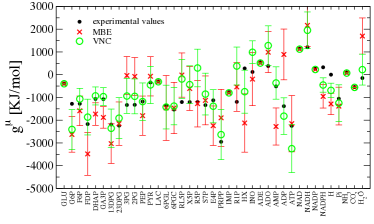
Figure 1: Chemical potentials of metabolites in the hRBC metabolic network computed by Method (a) with poor input information: experimental estimates (black markers) and values obtained for MBE (red markers) and VNC (green markers) direction assignments. The initial spread of chemical potentials encoded in $P_{0}$ (spanning either the $[0,2000]$ or the $[-5000,0]$ range) is not shown. The errors on the experimental estimates of the fixed chemical potentials fall within the size of the dots.

Both mass-balance conditions turn out to provide thermodynamically feasible configurations of reaction directions and in both cases one obtains a broad agreement between computed and experimentally measured chemical potentials. This shows that Method (a), apart from being able to verify the thermodynamic feasibility of a flux state, is able to retrieve information on the energy landscape. Keeping in mind that MBE represent tighter constraints on fluxes than VNC and that the networks used in [12] and [24] are not identical (specifically in uptakes), one sees that the directions extracted from (3) slightly outperform those resulting from (2) in predicting chemical potentials, while both fail to predict (via Method (a)) the $g^{\mu}$’s of key metabolites like NADH and NADPH. The magnitude of the error bars reflects the considerable initial uncertainty we have assumed in the input information, as prior knowledge in this case is the minimal needed to solve (26) unambiguously.

IV.2 Method (a), rich input information

A much refined prediction is obtained using a rich input information. Results are displayed in Fig. 2.

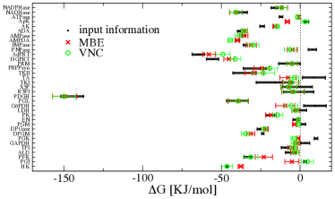
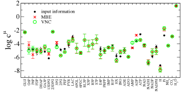
Figure 2: Predictions obtained for the hRBC network by Method (a) with rich input information. Top: free energy changes: input information with error (black markers) and values obtained for MBE (red markers) and VNC (green markers) direction assignments. Bottom: measured metabolite (log-)concentrations: input information with error (black markers) and values obtained for MBE (red markers) and VNC (green markers) direction assignments.

The computed affinities display significant changes with respect to the picture embedded in $P_{0}$. For instance, several of the initial bounds on affinities indicate that the free energy change in a reaction is positive (e.g. PGI, PGK, G6PDH, TA), due either to the actual experimental estimates for the affinities or to the initial uncertainty we place on concentrations. Such bounds are altered by MinOver in a direction compatible with physiologic assignments (see Table S2), suggesting that the implementation of Method (a) correlates the fluctuations of chemical potentials. At the same time, we observe that in some cases fluctuations of $g^{\mu}$ exceed the initial boxes defined by $P_{0}$. Since the resulting ranges are compatible with the intake configuration, they may provide an estimate of the statistical fluctuations from cell to cell. This also allows to obtain an estimate for the concentration range, including for metabolites whose level has not been experimentally probed (6PGL, RL5P, X5P, R5P, S7P). Our predictions for the levels of (1,3)-diphosphoglycerate ($(1,3)$-DPG), 2-phosphoglycerate (2PG) and phosphoenolpyruvate (PEP) differ from the experimental estimates. This is a consequence of the fact that we are forcing the phosphoglycerate kinase (PGK) and the glyceraldehyde phosphate dehydrogenase (GAPDH) reactions in the forward direction, in agreement with the steady state direction assignments for glycolysis, even if the experimental values would classify them as reversible. In addition, we obtain different levels of key metabolites like ATP and inorganic phosphate, while our predictions for ADP and AMP fail in the MBE and VNC conditions, respectively. This can be partially traced back to the difficulties inherent in assessing the potentials of highly exchanged metabolites [23]. On the other hand, the experimental estimates of these concentrations vary considerably across the literature (e.g. [27] vs [28]). Finally, a net intake of phosphate groups and a net outtake of CO₂ is predicted both for the MBE and the VNC states even if in physiological conditions the ratio of internal concentrations and the external levels in the blood would suggest otherwise (see Tables S1 and S3). This, together with a slight inconsistency in the pH level, seems to call for the inclusion in the network of the carbonic anhydrase (CA-I) reaction, as well as of a bicarbonate (HCO${}_{3}^{-}$) outtake. The former carries out the intracellular pH buffering by hydrating CO₂ into bicarbonate, while the latter releases HCO${}_{3}^{-}$ through the BAND3 membrane protein, which can cover up to 25% of the membrane surface [29]. So, even if in the standard biochemical state species that differ only by the hydration level are usually lumped together in the reactants list, we have chosen to treat carbon dioxide and bicarbonate as different metabolites in the implementation of Method (b).

IV.3 Method (b), rich input information

Results obtained by Method (b) (without a priori assumptions on reversibility) are displayed in Figs. 3 and 4.

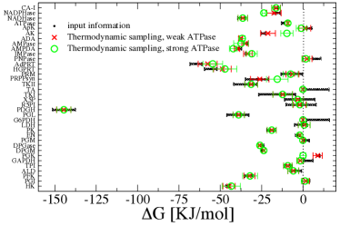
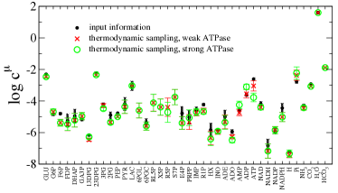
Figure 3: Predictions obtained for the hRBC network by Method (b) with rich input information. Top: free energy changes: input information with error (black markers) and values obtained for MBE (red markers) and VNC (green markers) direction assignments. Bottom: measured metabolite (log-)concentrations: input information with error (black markers) and values obtained for MBE (red markers) and VNC (green markers) direction assignments.

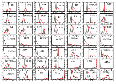
Figure 4: Marginal distributions of fluxes for the hRBC network obtained by Method (b) with rich input information under strong (red lines) and weak (black lines) ATPase flux. The reference unit for fluxes is fixed to the measured value of GLC uptake, namely $4\cdot 10^{-6}\text{mol/s}$.

Because the ATPase pump turns out to be weakly active across the solution space (as in [24]), we have performed a second set of calculations forcing a strong flux through it (comparable with the GLC uptake, as in[12]). In the former case, compared to the Monte Carlo sampling of [12] two more reactions are found to be effectively bidirectional in agreement with their standard assignment, i.e. PGK and lactate dehydrogenase (LDH). Note that when the former is operating backward, it activates a futile cycle with the Rapoport-Luebering shunt, a behavior that has been experimentally observed in acidic conditions [30]. When ATPase flux is large, instead, PGK is constrained in the forward direction. On the other hand, reverse LDH implies a LAC intake and a higher flux of NADHase. Simple biochemical arguments (see Section S5) suggest that the physiologically relevant scenario for hRBCs is that where the ATPase flux is much smaller than the GLC uptake. We shall henceforth focus on this case (corresponding results for strong ATPase flux are reported in Sec. S4).

The pairwise correlations among fluxes (Fig. 5) show that glycolysis and the pentose-phosphate pathway form tight modules that are weakly anti-correlated with each other, mostly through the reversible phosphoglucoisomerase (PGI) reaction.

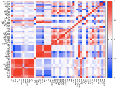
Figure 5: Pearson coefficients of the fluxes obtained by Method (b) with rich input information under weak ATPase flux.

The forward (resp. backward) direction of PGI indeed indicates that glucose is processed preferentially through glycolysis (resp. pentose phosphate pathway). Glycolysis can furthermore be broken down into two separated blocks with a weaker (positive) cross-correlation. The nucleotides salvage pathway forms instead a weakly correlated module. The network ultimately presents six bidirectional reactions (PGI, PGK, LDH, R5PI, ApK, LACe). Comparing Figs. 4 and 5 one sees that the directions of PGK, LDH and PGI govern the state of ATPase, NADHase and NADPHase, respectively. For instance, the negative (resp. positive) part of the LDH distribution corresponds to the high (resp. low) flux state of the NADHase pump (LDH and NADHase are strongly anticorrelated).

IV.4 Chemical potential correlations

We hinted above that the coupling of (3) and (26) generates non trivial correlations between the chemical potentials in feasible states in both Methods (a) and (b). A quantitative look at this aspect is reported in Fig. 6.

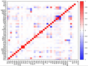
Figure 6: Pearson coefficients of the chemical potentials obtained by Method (b) with rich input information under weak ATPase flux.

Note that correlations were initially absent, since $P_{0}(\mathbf{g})$ is assumed to be a product of uncorrelated independent distributions. The algorithmic origin of such interdependecies can be understood considering that chemical potentials are updated dynamically through a series of reinforcement steps of the form $\alpha s_{i}\xi^{\mu}_{i}$. It follows that the $g^{\mu}$’s can ultimately be written as $g^{\mu}=g^{\mu}_{\text{tr}}+\alpha\sum_{i}k_{i}\xi^{\mu}_{i}$, where $g_{\text{tr}}^{\mu}$ is the trial chemical potential sampled from $P_{0}$ and $k_{i}$ is an index which is updated (increased or decreased by one according to the sign of the reaction) each time reaction $i$ tries to invert. The covariance between chemical potentials can thus be decomposed as

$$\langle g^{\mu}g^{\nu}\rangle_{c}=\delta_{\mu\nu}\sigma^{2}_{\mu}+\alpha\sum_{i=1}^{N}\xi_{i}^{\mu}\langle g_{\text{tr}}^{\nu}k_{i}\rangle_{c}+\alpha\sum_{i=1}^{N}\xi_{i}^{\nu}\langle g_{\text{tr}}^{\mu}k_{i}\rangle_{c}+\alpha^{2}\sum_{i,j}\xi_{i}^{\mu}\xi_{j}^{\nu}\langle k_{i}k_{j}\rangle_{c}$$ (15)

where $\langle.\rangle_{c}$ stands for the connected correlation, $\sigma_{\mu}^{2}$ is the variance of $P_{0}^{\mu}$, so that $\langle g_{\text{tr}}^{\mu}g_{\text{tr}}^{\nu}\rangle_{c}=\delta_{\mu\nu}\sigma^{2}_{\mu}$. Neglecting correlations between $k_{i}$ and $k_{j}$ for $i\neq j$ and between $g_{\text{tr}}^{\mu}$ and $k_{i}$ (for each $\mu$ and $i$) this reduces to

$$\langle g^{\mu}g^{\nu}\rangle_{c}\simeq\alpha^{2}\sum_{i=1}^{N}\xi_{i}^{\mu}\xi_{i}^{\nu}\sigma^{2}_{k_{i}}~{}~{}~{}~{}~{}(\mu\neq\nu)\;.$$ (16)

This simply tells us that the dynamics tends to correlate (resp. anti-correlate) metabolites typically appearing on the same (resp. opposite) side of the reaction equations (such as ADP and ATP).

In this respect, it is worthwhile to compute the amount of information gained (or lost) through the sampling algorithms essentially via the build-up of correlations. Note that indeed, since input distributions can be dynamically broadened, a loss of information is actually possible. The rationale behind this flexibility is that we are interested in estimating the ranges of variability of single cell states, which may exceed the uncertainty derived from experimental measures that are typically performed by averaging over a large number of cells. Now the information gain is related to the difference in entropy of the initial and final distributions, which is particularly simple to estimate assuming to be dealing with Gaussian distributions. Indeed the entropy of a Gaussian $Q(\mathbf{g})$ is given by [31]

$$S[Q(\textbf{g})]=\frac{1}{2}\text{tr}[\log(\textbf{K})]+\frac{M}{2}[1+\log(2\pi)]$$ (17)

where K is the covariance matrix of the $g^{\mu}$’s and $M$ is the dimensionality of the space, i.e. the number of metabolites. It follows that

$$I=-(S[P(\textbf{g})]-S[P_{0}(\textbf{g})])=\frac{1}{2}\sum_{\mu=1}^{M}[\log(\lambda^{\mu}_{0})-\log(\lambda^{\mu})]\;,$$ (18)

where $\lambda_{0}^{\mu}$ and $\lambda^{\mu}$ are respectively the eigenvalues of the covariance matrix for the initial and final distributions, is the information gain. Surprisingly, the information gain thus computed is found to be negative ($I\simeq-3.98$) for Method (a), and positive ($I\simeq 4.12$) for Method (b), indicating that the thermodynamic sampling algorithm allows for a refinement of the input information. The rank plot of eigenvalues (see Fig. S5) shows clearly that Method (a) is capable of extracting information only from the metabolites with largest $\mathbf{K}$ eigenvalues (associated with highly uncertain concentrations) and is generically outperformed by Method (b).

In order to spot key-metabolites whose concentration variability bears a strong influence on the global organization of fluxes, we can quantify the correlations between fluxes and concentrations emerging from Method (b) by computing the index

$$\chi_{i}^{\mu}=\frac{\left\langle(\nu_{i}-\left\langle\nu_{i}\right\rangle)(g^{\mu}-\left\langle g^{\mu}\right\rangle)\right\rangle}{\sqrt{\left\langle(\nu_{i}-\left\langle\nu_{i}\right\rangle)^{2}\right\rangle\left\langle(g^{\mu}-\left\langle g^{\mu}\right\rangle)^{2}\right\rangle}}\;~{},$$ (19)

which correlates the fluctuations in chemical potentials to those in fluxes. This matrix is shown in Fig. 7.

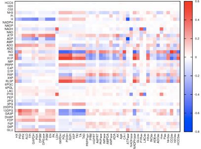
Figure 7: Correlations between chemical potentials and fluxes (see (19)) obtained by Method (b) with rich input information under weak ATPase flux.

High concentrations of (1,3)-DPG and GA3P appear to favor the glycolytic pathway over the pentose-phosphate pathway, whereas the nucleotide rescue pathways is activated by high levels of INO and R5P and low levels of HX and R1P, whose concentration is instead correlated with high flux through the pentose-phosphate group. Note that concentrations of metabolites only appearing in far from equilibrium reactions (like (2,3)-DPG) are seldom modified by the algorithm and thus appear to be particularly stable, as the corresponding $\chi_{i}^{\mu}$ are weakly dependent on fluxes.

IV.5 Chemical energy balance

The network nodes that are more tightly connected to the biological functionality of the haematids are the three $ase$ pumps: ATPase (that regulates the internal osmotic pressure and the transmembrane potential), NADHase (that reduces hemoglobin from its metastable state) and NADPHase (that maintains the redox state of the cell by reducing glutathione). Their respective work loads can be estimated from basic biochemical parameters.

The work carried out by the ATPase pump can be written as

$$W_{\text{ATP}}=-FV_{0}+RT\left[3\log\frac{c_{\text{Na}^{+}_{(ext)}}}{c_{\text{Na}^{+}_{(in)}}}+2\log\frac{c_{\text{K}^{+}_{(in)}}}{c_{\text{K}^{+}_{(ext)}}}\right]\;,$$ (20)

where $F\simeq 96~{}\text{KJ/(mol V)}$ is the Faraday constant and $V_{0}\simeq-12~{}\text{mV}$ is the transmembrane potential, while $c_{\text{Na}^{+}_{(ext)}}/c_{\text{Na}^{+}_{(in)}}\simeq 20$ and $c_{\text{K}^{+}_{(in)}}/c_{\text{K}^{+}_{(ext)}}\simeq 18$ are the ratios between external and internal levels of sodium and potassium ions. At $T=310\text{K}$, we obtain $W_{\text{ATP}}\simeq 50\text{ KJ/mol}$.

The work carried out by the NADHase pump, specifically by cytochrome b5 reductase, can instead be estimated from the standard values of the redox potential of the couple Fe${}^{2+}/$Fe³⁺ in the heme group of hemoglobin (namely $V_{1}\simeq 60\text{ mV}$ [28]) upon assuming normal levels of meta-hemoglobin ($2\%$ of the total). We obtain

$$W_{\text{NADH}}=-2FV_{1}+2RT\log\frac{c_{\text{Hb}}}{c_{\text{MetHb}}}\simeq 10\text{ KJ/mol}\;.$$ (21)

(The factor two comes from the fact that the reductase enzyme couples each NADHase with the reduction of two molecules of oxidized hemoglobin.)

Finally we can estimate the work done by the NADPHase pump, glutathione reductase, from the standard redox potential of the pair 2GSH/GSSG, i.e. $V_{2}\simeq-230mV$, and from their concentrations measured in human red cells, given respectively by $c_{\text{GSH}}\simeq 3.2\cdot 10^{-3}\text{ M}$, $c_{\text{GSSG}}\simeq 6.5\cdot 10^{-5}\text{ M}$ [28]. We find

$$W_{\text{NADPH}}=-FV_{2}+RT\log\frac{c_{\text{GSH}}^{2}}{c_{\text{GSSG}}}\simeq 55\text{ KJ/mol}.$$ (22)

The total amount of work per unit time performed by these three processes can now be written as

$$\dot{W}=\nu_{\text{ATPase}}W_{\text{ATP}}+\nu_{\text{NADHase}}W_{\text{NADH}}+\nu_{\text{NADPHase}}W_{\text{NADPH}}\;,$$ (23)

where $\nu_{\text{ATPase}}$ is the flux of ATPase (and similarly for the remaining pumps). At the same time, the entropy produced by the cell per unit time reads

$$T\dot{S}\equiv-\sum_{i\in R\setminus U}\nu_{i}\Delta G_{i}-\sum_{\mu\in U}u^{\mu}\cdot(g_{ext}^{\mu}-g^{\mu})-\dot{W}\;,$$ (24)

where the first sum coincides with the quadratic form defined by the stoichiometric matrix of intracellular reactions, i.e. $\sum_{i,\mu}\nu_{i}\xi_{i}^{\mu}g^{\mu}$, and the second is over cross-membrane transport processes (uptakes), with $u^{\mu}$ the uptake flux of metabolite $\mu$. In order to obtain a realistic description of the processes, after normalizing our computed fluxes with respect to the average value of the GLC uptake ($u\simeq 4\cdot 10^{-6}\text{ mol/(l s)}$ [32]), we scaled them by the cell volume ($V_{\text{hRBC}}\simeq 90\text{ fl}$). The naïve thermodynamic efficiency of the hRBC can finally be evaluated as

$$\eta=\frac{\dot{W}}{\dot{W}+T\dot{S}}$$ (25)

In Fig. 11 we display the distributions of $\dot{W}$, $T\dot{S}$, $\dot{U}=\dot{W}+T\dot{S}$ and $\eta$ obtained from Method (b) with weak and strong ATPase flux.

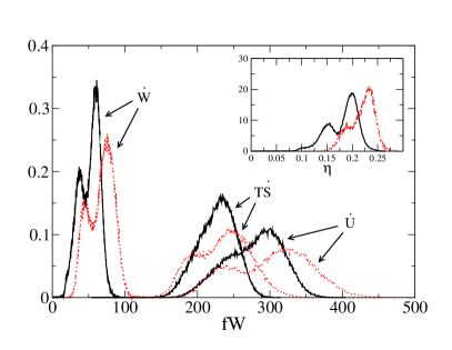
Figure 8: Distributions of work done ($\dot{W}$), entropy produced ($T\dot{S}$) and energy flow ($\dot{U}$) per unit time for the hRBC metabolism with strong (dotted line) and weak (straight line) ATPase flux. Inset: distribution of efficiency ($\eta$) in the same conditions.

The two peaks in the distributions mirror those appearing in the flux distributions of the NADH and NADPH pumps. Remarkably, the computed efficiency of the hRBC is not far from that corresponding to optimal microbial growth, which was estimated to be close to 24% [33]. Note that the work performed per unit time by the NADPHase pump dominates the sum (23). Therefore the two peaks appearing in the distribution of $\dot{W}$ mirror those appearing in the distribution of $\nu_{\text{NADPHase}}$.

V Conclusion

Constraint-based models of cellular metabolism are important tools to analyze and predict the chemical activity and response to perturbations of cells without relying on kinetic and transport details that are often unavailable. In such frameworks, assessing the metabolic capabilities of a cell requires the exploration of a high dimensional space representing flux and chemical potential configurations compatible with mass- and energy-balance constraints. The complexity of the ensuing problem can in some cases be reduced by applying reasonable (though necessarily ad hoc) optimality criteria. Most often, however, one needs to sample “physiological configurations” from the solution space starting from a priori biochemical knowledge that could be noisy. The methods proposed here are designed to retrieve distributions of fluxes and chemical potentials (or concentrations) essentially by exposing and building up correlations between variables. This is substantially different from other approaches (e.g. [10, 22]), where either the flux distributions compatible with given chemical potentials or the reverse are sought. Disposing of reliable prior biochemical information is obviously a limiting factor in our case as well. The advantage lies in the fact that working with correlations allows for a greater flexibility in treating the biochemical input data. Besides providing information on feasible physiological concentration ranges, flux distributions and reaction directionality, thermodynamic sampling can be employed to evaluate the responsiveness of fluxes to fluctuations in concentrations (or the reverse) and to assess the thermodynamic efficiency of a cell. In the case considered here (the hRBC, where a comparison with results obtained by sampling the solution space of mass-balance equations is possible), we have estimated $\eta\simeq 0.24$ assuming that the functional core of its metabolism lies in the three pumps (ATPase, NADHase, NADPHase). A similar calculation can be carried out on more complex genome-scale systems (e.g. E. coli) for a modest increase of computational costs (work in progress).

Appendix A Role of thermodynamic constraints: a simple example

In order to clarify how thermodynamic constraints translate into bounds on the degrees of freedom, consider the small module shown in Fig. 9. A priori, it admits $2^{5}=32$ different direction assignments, corresponding to the 8 possible states for the 3 internal fluxes $x$, $y$ and $z$, times the 4 possible states of the boundary fluxes $u$ and $v$.

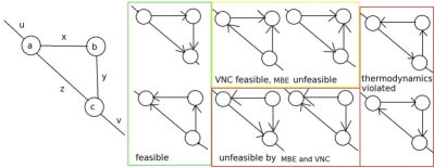
Figure 9: Network module with $3$ internal reactions, $x$, $y$ and $z$ between $3$ chemical species $a$, $b$ and $c$ and $2$ uptake fluxes $u$ and $v$. Unit stoichiometry is assumed.

Assuming unit stoichiometry, one easily sees that 6 of the 8 states allowed for $(x,y,z)$ are thermodynamically feasible, corresponding to the number of ways in which one can order the chemical potentials of metabolites $a$, $b$ and $c$. The excluded configurations present unfeasible cycles. Mass constraints further reduce the space of possible directions. Mass-balance equations (MBE) impose that each metabolite should be produced and consumed by at least one reaction, leaving only two feasible direction assignments. The softer Von Neumann conditions (VNC) instead force each metabolite to be produced at least by one reaction, leaving four possible states. Once the possible directions of the boundary fluxes $u$ and $v$ are considered, one ends up with two thermodynamically and stoichiometrically feasible configurations for MBE and eight for VNC (down from 32).

Now let us focus on a specific flux model (say MBE) and note that it enforces $u=v$, $x=y$ and $v=x+z$. This leaves two free parameters, e.g. $v$ and $x-z=\lambda$, and it is easy to show that the exclusion of unfeasible cycles implies $|\lambda|\leq u$. Similar though more lengthy arguments can be formulated for the Von Neumann flux model VNC.

Further examples are discussed e.g. in [7, 34].

Appendix B hRBC data

The hRBC metabolic network employed for this study is shown in Fig. 10.

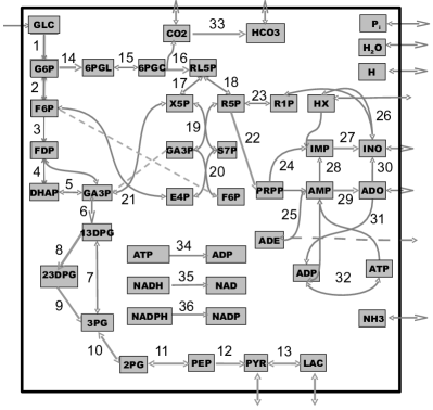
Figure 10: The hRBC network employed in this study.

It is formed by $40$ metabolites (listed in Table 1) interacting through $35$ intracellular reactions (listed in Table 2) and subject to $12$ (for Method (a)) or 13 (for Method (b)) uptakes. (Bicarbonate outtake was only accounted for in Method (b).) The network can be divided in three main pathways, namely glycolysis (reactions 1-13), the pentose phosphate pathway (reactions 14-21), and a nucleotide salvage pathway (reactions 22-32). The directions displayed correspond to the standard physiological assignment. The network coincides with the reconstruction presented in [12], except for the inclusion of bicarbonate (HCO${}_{3}^{-}$), of the carbonic anhydrase reaction (33) and of a bicarbonate uptake. Table 1 also provides the standard chemical potential for each metabolite and an estimate of the intracellular concentration (when available). Potentials are computed in the standard biochemical state, i.e. in acqueous solution at fixed temperature, pressure, ionic strength and pH and are available in [22], where they are calculated according to the prescriptions of [35, 36] at $T=298$ K, $P=1$ atm, pH $=7.6$ and ionic strenght I $=0.15$ M. The physiological conditions of the hRBC are known to be slightly different ($T=310$ K, pH $=7.2$), but such differences do not affect significantly the results of our procedures. The estimated intracellular concentration ranges are obtained from measurements in different settings. It is worth to notice that the experimental errors on such values of concentrations reflect an essential uncertainty rather than statistical fluctuations from cell to cell, since standard measurements of concentrations are usually carried out averaging over many ($10^{2}-10^{8}$) cells.

Abbr.	Compound name	$g_{0}$ [KJ/mol]	$c$ [M]
GLC∗	Glucose	$-387$	$5\pm 1\cdot 10^{-3}$ [27]
G6P	Glucose-6-phosphate	$-1281$	$4\pm 1\cdot 10^{-5}$ [27]
F6P	Fructose-6-phosphate	$-1278$	$1.3\pm 0.5\cdot 10^{-5}$ [27]
FDP	Fructose-1,6-diphosphate	$-2171$	$2.7\pm 1\cdot 10^{-6}$ [27]
DHAP	Dihydorxyacetone phosphate	$-1070$	$1.7\pm 0.1\cdot 10^{-5}$ [39]
GA3P	Glyceraldehyde-3-phosphate	$-1078$	$5.7\pm 1\cdot 10^{-6}$ [39]
13DPG	1,3-Diphosphoglycerate	$-2191$	$1\pm 0.5\cdot 10^{-6}$ [40]
23DPG	2,3-Diphosphoglycerate	$-2240$	$4\pm 3\cdot 10^{-3}$ [40]
3PG	3-Phosphoglycerate	$-1332$	$4\pm 2\cdot 10^{-5}$ [39]
2PG	2-Phosphoglycerate	$-1326$	$1.4\pm 0.5\cdot 10^{-5}$ [39]
PEP	Phosphoenolpyruvate	$-1181$	$1.7\pm 0.2\cdot 10^{-5}$ [27]
PYR∗	Pyruvate	$-341$	$8\pm 6\cdot 10^{-5}$ [39]
LAC∗	Lactate	$-297$	$1.4\pm 0.5\cdot 10^{-3}$ [27]
6PGL	6-Phosphogluco-lactone	$-1352$
6PGC	6-Phosphogluconate	$-1353$	$5\pm 2\cdot 10^{-6}$ [41]
RL5P	Ribulose-5-phosphate	$-1201$
X5P	Xylusose-5-phosphate	$-1203$
R5P	Ribose-5-phosphate	$-1202$
S7P	Sedoheptulose-7-phosphate	$-1336$
E4P	Erythrose-4-phosphate	$-1125$	$5\pm 2\cdot 10^{-5}$ [42]
PRPP	5-Phosphoribosyl-1-pyrophosphate	$-2949$	$5\pm 1\cdot 10^{-5}$ [38]
IMP	Inosine monophosphate	$-774$	$3\pm 1\cdot 10^{-5}$ [43, 44]
R1P	Ribose-1-phosphate	$-1194$	$6\pm 5\cdot 10^{-6}$
HX∗	Hypoxanthine	$274$	$2\pm 1\cdot 10^{-6}$ [38]
INO∗	Inosine	$119$	$1.3\pm 0.5\cdot 10^{-6}$ [38]
ADE∗	Adenine	$538$	$1.3\pm 0.7\cdot 10^{-5}$ [38]
ADO∗	Adenosine	$378$	$1.3\pm 0.3\cdot 10^{-6}$ [38]
AMP	Adenosine monophosphate	$-514$	$8\pm 1\cdot 10^{-4}$ [28]
ADP	Adenosine diphosphate	$-1384$	$1.0\pm 0.1\cdot 10^{-3}$ [28]
ATP	Adenosine triphosphate	$-2250$	$7.9\pm 0.1\cdot 10^{-3}$ [28]
NAD	Nicotinamide adenine dinucleotide	$1145$	$7\pm 2\cdot 10^{-5}$[39]
NADH	Nicotinamide adenine dinucleotide(R)	$1209$	around $10^{-7}$ (ext)
NADP	Nicotinamide adenine dinucleotide phosphate	$260$	$1.4\pm 0.5\cdot 10^{-6}$ [45]
NADPH	Nicotinamide adenine dinucleotide phosphate (R)	$325$	$4\pm 2\cdot 10^{-5}$ [45]
H∗	Hydrogen ion	$0$	$10^{-7.2}$ [46]
Pi∗	Inorganic phosphate	$-1055$	$1.0\pm 0.5\cdot 10^{-3}$ [28]
NH${}_{3}^{*}$	Ammonia	$96$	$5\pm 1\cdot 10^{-5}$ [47]
CO${}_{2}^{*}$	Carbon dioxide	$-543$	$1.2\pm 0.5\cdot 10^{-3}$ [48]
H2O∗	Water	$-149$	solvent
HCO${}_{3}^{*}$	Bicarbonate	$-710$	$1.6\pm 0.1\cdot 10^{-2}$ [48]

Table 1: Metabolites included in the human red blood cell metabolic network used in this study. $g_{0}$ represents the standard chemical potential of the metabolite, while $c$ denotes an indicative value for the experimentally estimated intracellular concentration, when available. Compounds marked by an asterisk are subject to uptakes. All data were searched through the Bionumbers database [38]; pointers to explicit references are given when available.

Nr	Abbr	Enzyme	reaction
1	HK	Hexokinase	$GLC+ATP\to G6P+ADP+H$
2	PGI	Phosphoglucoisomerase	$G6P\leftrightarrow F6P$
3	PFK	Phosphofructokinase	$F6P+ATP\to FDP+ADP+H$
4	ALD	Aldolase	$FDP\leftrightarrow GA3P+DHAP$
5	TPI	Triose phosphate isomerase	$DHAP\leftrightarrow GA3P$
6	GAPDH	GLyceraldehyde phosphate dhydrogenase	$GA3P+NAD+Pi\leftrightarrow 13DPG+NADH+H$
7	PGK	Phosphoglycerate kinase	$13DPG+ADP\leftrightarrow 3PG+ATP$
8	DPGM	Diphosphoglyceromutase	$13DPG\to 23DPG+H$
9	DPGase	Diphosphoglycerate phosphatase	$23DPG+H_{2}O\to 3PG+Pi$
10	PGM	Phosphoglyceromutase	$3PG\leftrightarrow 2PG$
11	EN	Enolase	$2PG\leftrightarrow PEP+H_{2}O$
12	PK	Pyruvate kinase	$PEP+ADP+H\to PYR+ATP$
13	LDH	Lactate dehydrogenase	$PYR+NADH+H\leftrightarrow LAC+NAD$
14	G6PDH	Glucose-6-phosphate dehydrogenase	$G6P+NADP\to 6PGL+NADPH+H$
15	PGL	6-phosphoglyconolactonase	$6PGL+H_{2}O\leftrightarrow 6PGC+H$
16	PDGH	6-phosphoglycoconate dehydrogenase	$6PGC+NADP\to RL5P+NADPH+CO_{2}$
17	R5PI	Ribose-5-phosphate isomerase	$RL5P\leftrightarrow R5P$
18	X5P	Xylulose-5-phosphate epimerase	$RL5P\leftrightarrow X5P$
19	TKI	Transketolase I	$X5P+R5P\leftrightarrow S7P+GA3P$
20	TA	Transaldolase	$GA3P+S7P\leftrightarrow E4P+F6P$
21	TKII	Transketolase	$X5P+E4P\leftrightarrow F6P+GA3P$
22	PRPPsyn	Phosphoribosyl pyrophosphate synthetase	$R5P+ATP\to PRPP+AMP$
23	PRM	Phosphoribomutase	$R1P\leftrightarrow R5P$
24	HGPRT	Hypoxanthine guanine phosphoryl transferase	$PRPP+HX+H_{2}O\to IMP+2Pi$
25	AdPRT	Adenine phosphoribosyl transferase	$PRPP+ADE+H_{2}O\to AMP+2Pi$
26	PNPase	Purine nucleoside phosphorylase	$INO+Pi\leftrightarrow HX+R1P$
27	IMPase	Inosine monophosphatase	$IMP+H_{2}O\to INO+Pi+H$
28	AMPDA	Adenosine monophosphate deaminase	$AMP+H_{2}O\to IMP+NH_{3}$
29	AMPase	Adenosine monophosphate phosphohydrolase	$AMP+H_{2}O\to ADO+Pi+H$
30	ADA	Adenosine deaminase	$ADO+H_{2}O\to INO+NH_{3}$
31	AK	Adenosine kinase	$ADO+ATP\to ADP+AMP$
32	ApK	Adenylate kinase	$2ADP\leftrightarrow ATP+AMP$
33	CA-I	Carbonic anhydrase	$CO_{2}+H_{2}O\leftrightarrow HCO_{3}+H$
34	ATPase	Sodium-Potassium ionic pump	$ATP+H_{2}O\to ADP+Pi$
35	NADHase	Cytochrome-b5 reductase	$NADH\to NAD+H$
36	NADPHase	Glutathion reductase	$NADPH\to NADP+H$

Table 2: Intracellular reactions included in the human red blood cell metabolic network used in this study.

Finally, in Table 3 we report the reference values for blood tests [37] of the level of metabolites of interest in serum.

Compound	Range (M)
GLC	$4-6\cdot 10^{-3}$
PYR	$3-10\cdot 10^{-5}$
LAC	$0.5-2.2\cdot 10^{-3}$
H+	$10^{-7.3}-10^{-7.45}$
Pi	$0.8-1.5\cdot 10^{-3}$
NH3	$1-6\cdot 10^{-5}$
CO2	$2-3\cdot 10^{-2}$
HCO${}_{3}^{-}$	$1.8-2.3\cdot 10^{-2}$

Table 3: Estimated concentration levels in blood serum.

Appendix C Details on the implementation of Methods (a) and (b)

Here we discuss in some detail four aspects connected to the implementation of Methods (a) and (b), namely

• the minimal amount of input information on chemical potentials (to be included in $P_{0}(\mathbf{g})$) needed to reconstruct the free energy landscape via Method (a);

• the form of the input information on chemical potentials (i.e. of $P_{0}(\mathbf{g})$) in the poor versus rich input information scenarios;

• the form of the input information on reaction directions sampled from MBE and VNC, required by Method (a) only;

• the choice of the “learning parameters” $\alpha$ and $\beta$ that appear, respectively, in both methods and in Method (b) only, that characterize the size of the update step in, respectively, chemical potentials and fluxes.

C.1 Minimal input information on chemical potentials

To begin with, let us note that the thermodynamic constraint

$$-\text{sign}(\nu_{i})\sum_{\mu=1}^{N}\xi_{i}^{\mu}g^{\mu}\geq 0$$ (26)

imposes that the chemical potential of metabolites that are sources (resp. sinks) of the network should be known, since the constraints (26) do not bound the corresponding $g^{\mu}$’s from above (resp. below). Clearly, then, computing the landscape of chemical potentials is feasible only if $P_{0}(\mathbf{g})$ carries some prior information on the $g^{\mu}$’s.

Besides network ‘leaves’, one easily sees that certain intracellular potentials should be known as well. Consider a chemical potential vector $\mathbf{g}_{\star}=\{g^{\mu}_{\star}\}$ that satisfies (26) and note that $\mathbf{g}_{\star}+k\boldsymbol{\lambda}$ is again a solution for $k\in\mathbb{R}$ provided $\boldsymbol{\lambda}=\{\lambda^{\mu}\}$ is such that $\sum_{\mu=1}^{M}\lambda^{\mu}\xi_{i}^{\mu}=0$ for each $i$. This degeneracy is related to the existence of equilibrium states and needs to be lifted. Ideally this can be achieved by fixing the chemical potentials of at least one of the metabolites with $\lambda^{\mu}\neq 0$ for each vector $\boldsymbol{\lambda}$ of the type described above. Note that such vectors include (but are not limited to) the conserved metabolic pools defined in [49]. A conserved pool is a group $P$ of metabolites described by a vector $\boldsymbol{\ell}=\{\ell^{\mu}\}$ with $\ell^{\mu}>0$ if $\mu\in P$, and zero otherwise, such that, for each $i$, $\sum_{\mu=1}^{M}\ell^{\mu}\xi_{i}^{\mu}=0$. From a physical viewpoint, each such pool corresponds to a conservation law for the aggregate concentration of the corresponding metabolites and the existence of one pool suffices to force $y^{\mu}=0$ for each $\mu\in P$ in the VNC scenario (in other words, metabolites belonging to conserved pools can not be producible) [50]. The simplest way to rule out equilibrium solutions is to clamp the chemical potential of a group $P^{\prime}$ of metabolites (including network sources and sinks) such that the problem

$$\sum_{\mu=1}^{M}\lambda^{\mu}\xi_{i}^{\mu}=\sum_{\mu\notin P^{\prime}}\lambda^{\mu}\xi_{i}^{\mu}+\sum_{\mu\in P^{\prime}}\lambda^{\mu}\xi_{i}^{\mu}=0~{}~{}~{}~{}~{}\forall i$$ (27)

admits no solution. From a geometrical perspective, the minimal number of metabolites whose chemical potentials needs to be constrained is that for which the number of independent equations in the above system exceeds the number of variables.

C.2 Poor versus rich input information

In the case of the hRBC, there are four source/sink nodes, namely glucose (GLC), lactate (LAC), ammonia (NH₃) and carbon dioxide (CO₂), whereas a basis for the left kernel of the stoichiometric matrix $\boldsymbol{\Xi}$ (excluding uptakes) turns out to be composed by seven vectors: $3$ conserved pools, namely the pairs (NAD, NADH) and (NADP, NADPH) and the larger pool formed by (HX, INO, IMP, ADE, ADO, AMP, ADP, ATP), plus $4$ other vectors whose components are related in a non-intuitive way to the balance of global quantities like the number of carbon atoms and phosphate groups. Analyzing (27), however, one finds that by clamping four metabolites (besides leaves) no equilibrium solution can exist.

In the poor input information scenario, we have therefore constructed $P_{0}(\mathbf{g})$ by fixing the chemical potentials of GLC, LAC, NH₃ and CO₂ as well as of inosine monophosphate (IMP), adenine (ADE), NAD, and NADP to remove the degeneracy associated to the presence of equilibrium solutions (different choices for these do not alter results). For these metabolites, $P_{0}^{\mu}(g^{\mu})=\delta(g^{\mu}-g^{\mu}_{\text{exp}})$, where $g^{\mu}_{\text{exp}}$ is the chemical potential obtained from experimental data. For the other compounds we have chosen a $P_{0}^{\mu}$ that reproduces the overall statistics of chemical potentials. In particular, each $g^{\mu}$ (in units of KJ/mol) is selected independently and uniformly in $[0,2000]$ with probability $p=0.2$ and in $[-5000,0]$ with probability $1-p=0.8$.

In the rich input information scenario, $P(\mathbf{g})$ was constructed as follows. The chemical potential of metabolites whose intracellular concentrations are known experimentally were extracted from the formula $g^{\mu}=g_{0}^{\mu}+RT\log c^{\mu}$. Here $g_{0}^{\mu}$ is the free energy of formation of the metabolite $\mu$ in the standard biochemical state. These values are accurately known for metabolites in the hRBC metabolic network (see Table 1). The concentrations $c^{\mu}$ are instead taken to be uniformly and independently distributed random variables with average values and box sizes according to the experimental estimates reported in Table 1. The concentrations of metabolites for which we were unable to find reliable experimental estimates are assumed to be uniformly and independently distributed random variables centered around $10^{-4}$ M and spanning four orders of magnitude symmetrically around the mean. Note that in this case no metabolite has a clamped chemical potential and the algorithm can modify the trial distributions of all metabolites.

In both scenarios, the chemical potential of water is treated as a boundary condition, i.e. it is kept fixed since we assume that water is in a condensed phase.

C.3 Input information for Method (a) on directions sampled from MBE and VNC

In [12] and [24], the hRBC network is assumed to operate under the MBE and VNC scenarios, respectively, in both cases starting from prior assignments for reaction directions. The implementation of Method (a) makes use of the reaction directions obtained in these studies. In summary:

• according to MBE, the net flux of all reactions is in the forward direction, except PGI, R5PI and ApK, (which are found to operate bidirectionally);

• according to VNC, the net flux of all reactions is in the forward direction, except R5PI (which is found to be operating bidirectionally), and PGI and ApK (which are found to operate in the backward direction).

For comparison the thermodynamic sampling Method (b) (which doesn’t require a priori reversibility assumptions) provides solutions in which the net flux of all reactions is in the forward direction, except PGI, PGK, LDH, R5PI and ApK (which are found to operate bidirectionally). Note that reverse PGK activates a futile cycle with the Rapoport-Luebering shunt. This behavior has been experimentally observed in acidic conditions [30].

It should be noted however that the network used here presents an additional intracellular reaction (CA-I), an additional metabolite (HCO${}_{3}^{-}$) and an additional uptake with respect to the networks studied above. Furthermore, the reconstructions employed in [12] and [24] have slight but important differences in the structure of uptakes.

C.4 Setting the learning rates

Both Methods (a) and (b) rely on learning rates (denoted as $\alpha$ for Method (a) and $\alpha$ and $\beta$ for Method (b)) that fix the size of the adjustment to be applied to chemical potentials ($\alpha$) and fluxes ($\beta$) at each iteration step.

For the implementation of Method (a) presented here, we set $\alpha$ to the (iteration-dependent) value $-2x_{i_{0}}/\sum_{\mu}(\xi_{i_{0}}^{\mu})^{2}$. One easily sees that if we let all the chemical potentials evolve during the sampling, this value of $\alpha$ has the net effect of reverting $x_{i_{0}}$ at each iteration while keeping the norm $\sum_{\mu}(g_{\mu})^{2}$, that defines the unit of the energy scale, constant. Note however that some of the chemical potentials must be kept fixed during the sampling (specifically those belonging to the set of compounds for which a priori information is required). In this case, the expression for $\alpha$ given above guarantees that the elementary step of the algorithm is proportional to the amount by which the constraint is violated. We found empirically that for this choice the convergence time decreases by a factor of about $10$ with respect to the case in which a constant $\alpha$ is employed.

In the implementation of Method (b) we chose the value $-2y_{\mu_{0}}/\sum(\xi_{i}^{\mu_{0}}(\rho))^{2}$ for $\beta$ (for the same reasons as above), while keeping a constant learning rate for chemical potentials ($\alpha=0.001$). This was motivated by the need to try to keep a “timescale” separation between the dynamics of fluxes and that of chemical potentials, with the latter preferentially slower than the former. In essence, this emphasizes the role of correlations in building up the solutions while potentially limiting the exploration of states to regions in the space of chemical potentials that are not too far from the initial states.

Finally, we remark that the solution space spanned by the completely reversible Von Neumann constraints may lack convexity for $\rho<1$ [26]. This leads to a certain rejection rate of solutions (roughly 10%), which represents a negligible additional cost in computations.

Appendix D Further results from Method (b)

Fig. 11 shows the flux-flux correlations computed from Method (b) assuming strong flux through the ATPase pump.

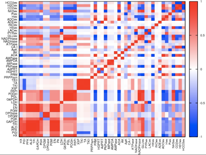
Figure 11: Pearson coefficients of the fluxes obtained by Method (b) with rich input information with strong ATPase flux.

Compared to the case where ATPase flux is weak, one notices that glycolysis is split in two separate but correlated modules, formed respectively by the first six and the last three reactions (in agreement with [12]). Similarly, the pentose phosphate pathway is split in two tight modules, while the nucleotides salvage pathway no longer forms a compact group. Note that the role of PGK and PGI as switches for the ATPase and NADPHase pumps is much less pronounced in this case.

The average production profile computed by Method (b) is displayed in Fig. 12.

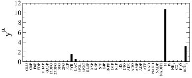
Figure 12: Average production profile obtained by jointly sampling fluxes and chemical potentials with ATPase ionic pump active. Note that fluxes are measured in units of GLC uptake.

One sees that all intracellular metabolites are mass-balanced except PYR, LAC, H⁺ and HCO${}_{3}^{-}$. This means that VNC solutions predict a slow steady growth of their concentration. However all of these are subject to outtakes, therefore the final state of the cell is globally mass balanced (i.e. the solutions of thermodynamically-constraint VNC would coincide with those of thermodynamically-constraint MBE on the same system).

The rank plot of the eigenvalues of the chemical potential correlation matrix $\mathbf{K}$ computed from Methods (a) and (b) is reported in Fig. 13.

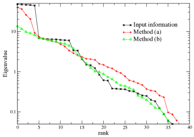
Figure 13: Rank plot of the eigenvalues of the correlation matrix of chemical potentials for $P_{0}(\mathbf{g})$ (black), and for the distributions obtained via Methods (a) (red) and (b) (green), for rich input information. Note that the $y$-scale is logarithmic.

One clearly sees that Method (b) outperforms Method (a) in gaining information over the trial distribution $P_{0}(\mathbf{g})$. Note in particular that Method (a) typically loses information on metabolites with small variability range in the trial distribution (corresponding to the smallest eigenvalues of $\mathbf{K}$).

Finally, Table 4 displays a summary of the chemical energy balance of the hRBC metabolism.

State	$T\dot{S}$(fW)	$\dot{W}$(fW)	$\dot{U}$(fW)	$\eta$
average eff., weak ATPase flux	226	51	278	0.18
average eff., strong ATPase flux	235	67	302	0.22
maximal eff., weak ATPase flux	256	92	348	0.264
maximal eff., strong ATPase flux	268	112	381	0.295

Table 4: Summary of the energy balance of the human red blood cell metabolic network

Appendix E Approximate energy balance analysis.

One of the results emerging from the sampling of fluxes and chemical potentials is that the overall flux through the nucleotide rescue pathway is about one order of magnitude lower than that going through glycolysis and/or pentose phosphate pathway. This is in agreement with previous results based on MBE and VNC without explicit thermodynamic constraints [24] and the known experimental values (see Table 5).

Reaction	Flux [M/s]
HK	$4.3\pm 0.7\cdot 10^{-6}$ [32]
GSSGR	$5\pm 1\cdot 10^{-5}$ [32]
RLS	$1.4\cdot 10^{-7}$ [51]
AMPcat	$3\cdot 10^{-9}$ [51]

Table 5: Measured fluxes in the red blood cell. GSSGR stands for glutathione reductase; RLS for Rapoport-Luebering shunt; AMPcat is AMP catalysis.

It is interesting to notice that in order to maintain the $ase$ pumps the activation of glycolysis and pentose phosphate pathway is sufficient. To see this, we can work out the stationary state of the network in absence of the nucleotide salvage pathway, i.e. for a reduced network consisting of 13 (glycolysis) + 8 (PPP) + 3 (pumps) = 24 intracellular reactions and 5 uptakes (GLC, PYR, LAC H₂O and HCO₃). The mass balance equations reveal that only four of the above reactions are linearly independent: we choose $u_{\text{GLC}}$, $u_{\text{LAC}}$ (glucose and lactate uptake), $\nu_{\text{G6PDH}}$ and $\nu_{\text{RLS}}$ (RLS stands for Rapoport-Luebering shunt). All fluxes can be written in terms of these. In particular, the quantities of interest in the energy balance take the form

$$\dot{U}=u_{\text{GLC}}(g^{\text{GLC}}_{(ext)}-2g^{\text{PYR}}_{(ext)})+u_{\text{LAC}}(g^{\text{LAC}}_{(ext)}-g^{\text{PYR}}_{(ext)})+\\ +\nu_{\text{G6PDH}}(1/3g^{\text{PYR}}_{(ext)}+2g^{\text{H${}_{2}$O}}_{(ext)}-g^{\text{HCO${}_{3}$}}_{(ext)})$$ (28)

for the energy flow and

$$\nu_{\text{ATPase}}=2u_{\text{GLC}}-\nu_{\text{G6PDH}}/3-\nu_{\text{RLS}}$$ (29)

$$\nu_{\text{NADHase}}=2u_{\text{GLC}}-\nu_{\text{G6PDH}}+u_{\text{LAC}}$$ (30)

$$\nu_{\text{NAPDHase}}=\nu_{\text{GSSGR}}=2\nu_{\text{G6PDH}}$$ (31)

for the fluxes through the pumps. Now under flux balance $u_{\text{GLC}}=\nu_{\text{HK}}$. Hence from the values in Table 5 we can estimate $\nu_{\text{ATPase}}\simeq 3\cdot 10^{-7}$ M/s, i.e. one order of magnitude smaller than the glucose uptake as in [24] and in agreement with our thermodynamic sampling without constraints on the ATP ionic pump.

References

- [1] T de Donder, L’Affinitè (Gauthier-Villars, Paris, 1927)
- [2] DA Beard and H Qian. Relationship between thermodynamic driving force and one-way fluxes in reversible chemical reactions. PLoS ONE 2 e144 (2007)
- [3] KJ Kauffman, P Prakash and JS Edwards. Advances in flux-balance analysis. Curr. Opin. Biotechnol. 14 491 (2003)
- [4] JD Orth, I Thiele and BØ Palsson. What is flux balance analysis? Nature Biotechnology 28 245 (2010)
- [5] R Schütz, L Kuepfer and U Sauer. Systematic evaluation of objective functions for predicting intracellular fluxes in Escherichia coli. Mol. Sys. Biol. 3 119 (2007)
- [6] AM Feist and BØ Palsson. The biomass objective function. Curr. Opin. Microbiol. 13 344 (2010)
- [7] D Beard, S Liang and H Qian. Energy balance for analysis of complex metabolic networks. Biophys. J. 83 79 (2002)
- [8] D Beard, E Babson, E Curtis and H Qian. Thermodynamic constraints for biochemical networks. J. Theor. Biology 228 327 (2004)
- [9] A Kümmel, S Panke and M Heinemann. Putative regulatory sites unraveled by network-embedded thermodynamic analysis of metabolome data. Mol. Sys. Biology 2 2006.0034 (2006)
- [10] A Hoppe, S Hoffmann and HG Holzhütter. Including metabolite concentrations into flux-balance analysis: thermodynamic realizability as a constraint on flux distributions in metabolic networks. BMC Systems Biology 1 23 (2007)
- [11] CS Henry, LJ Broadbelt and V Hatzimanikatis. Thermodynamics-based metabolic flux analysis. Biophys. J. 92 1792 (2007)
- [12] ND Price, J Schellenberger and BØ Palsson. Uniform sampling of steady-state flux spaces: means to design experiments and to interpret enzymopathies. Biophys. J. 87 2172 (2004)
- [13] A Braunstein, R Mulet and A Pagnani. Estimating the size of the solution space of metabolic networks. BMC Bioinformatics 9 240 (2008)
- [14] C Martelli, A De Martino, E Marinari, M Marsili and I Perez Castillo. Identifying essential genes in Escherichia coli from a metabolic optimization principle. Proc. Nat. Acad. Sci. USA 106 2607 (2009)
- [15] A De Martino, C Martelli, R Monasson and I Perez Castillo. Von Neumann’s expanding model on random graphs. J. Stat. Mech. [JSTAT] P05012 (2007)
- [16] RU Ibarra, JS Edwards and BØ Palsson. Escherichia coli K-12 undergoes adaptive evolution to achieve in silico predicted optimal growth. Nature 420 186 (2002)
- [17] D Segrè, D Vitkup and GM Church. Analysis of optimality in natural and perturbed metabolic networks. Proc. Natl. Acad. Sci. USA 99 15112 (2002)
- [18] T Shlomi, O Berkman and E Ruppin. Regulatory on/off minimization of metabolic flux changes after genetic perturbations. Proc. Natl. Acad. Sci. USA 102 7695 (2005)
- [19] M Imielinski, C Belta, H Rubin and A Halasz. Systematic analysis of conservation relations in E.coli genome-scale metabolic network reveals novel growth media. Biophys. J. 90 2659 (2006)
- [20] A De Martino and E Marinari. The solution space of metabolic networks: producibility, robustness and fluctuations. J. Phys. Conf. Ser. 233 012019 (2010)
- [21] J. Von Neumann. A model of general economic equilibrium. The Review of Economic Studies 13 1 (1945)
- [22] A Kümmel, S Panke and M Heinermann. Systematic assignment of thermodynamic constraints in metabolic network models. BMC Bionformatics 7 512 (2006)
- [23] RMT Fleming, I Thiele and HP Nasheuer. Quantitative assignment of reaction directionality in constraint-based models of metabolism: application to Escherichia coli. Biophys. Chem. 145 47 (2009)
- [24] A De Martino, D Granata, E Marinari, C Martelli and V Van Kerrebroeck. Optimal fluxes, reaction replaceability, and response to enzymopathies in the human red blood cell. J. Biomed. Biotechol. 2010 415148 (2010)
- [25] W Krauth and M Mézard. Learning algorithms with optimal stability in neural networks. J. Phys. A: Math. Gen. 20 L745 (1987)
- [26] A De Martino, M Figliuzzi and M Marsili. One way to grow, many ways to shrink: the reversible Von Neumann expanding model. J.Stat.Mech. [JSTAT] P07032 (2010)
- [27] E Beutler, Red cell metabolism: a manual of biochemical methods (Grune and Stratton, New York, 1984)
- [28] DL Nelson and MM Cox, Lehninger principles of biochemistry (WH Freeman & Co., New York, 2003)
- [29] NM Burton and LJ Bruce. Modelling the structure of the red cell membrane. Biochem Cell Biol. 89 200 (2011)
- [30] JA Black, KM Acott and L Bufton. A futile cycle in erythrocyte glycolysis. Biochim. Biophys. Acta 810 246 (1985)
- [31] N Misra, H Singh and E Demchuk. Estimation of the entropy of a multivariate normal distribution. J. Multivariate Analysis 92 324 (2005)
- [32] DR Thorburn and PW Kuchel (1985). Regulation of the human-erythrocyte hexose-monophosphate shunt under conditions of oxidative stress. A study using NMR spectroscopy, a kinetic isotope effect, a reconstituted system and computer simulation. Eur. J. Biochemistry 150 371 (1985)
- [33] HV Westerhoff, KJ Hellingwerf and K Van Dam. Thermodynamic efficiency of microbial growth is low, but optimal for maximal growth rate. Proc. Nat. Acad. Sci. USA 80 305 (1983)
- [34] D Beard and H Qian, Biophysical chemistry (Cambridge University Press, Cambridge UK, 2008)
- [35] RA Alberty, A Cornish-Bowden, RN Goldberg, GG Hammes, K Tipton and HV Westerhoff. Recommendations for terminology and databases for biochemical thermodynamics. Biophys. Chem. 155 89 (2011)
- [36] R Alberty, Thermodynamics of biochemical reactions (John Wiley and sons, Hoboken, NJ, 2003)
- [37] en.wikipedia.org/wiki/Reference_ranges_for_blood_tests
- [38] http://bionumbers.hms.harvard.edu/
- [39] G Jacobasch, S Minakami et al. Glycolysis of the erythrocyte. In Cellular and molecular biology of erythrocytes (Urban and Schwarzenberg, Munich, 1974)
- [40] R. Garrett and CM Grisham. Biochemistry (Thomson Brooks/Cole, Belmont, CA, 2005)
- [41] HN Kirkman and GF Gaetani. Regulation of glucose-6-phosphate dehydrogenase in human erythrocytes. J. Biol. Chem. 261 4033 (1986)
- [42] M Magnani, V Stocchi et al. Regulatory properties of rabbit red blood cell hexokinase at conditions close to physiological. Biochimica ett Biophysica Acta 804 145 (1984)
- [43] A Tomoda, K Yagawa et al. Accumulation of inosine 5’-monophosphate in human erythrocytes incubated with inosine. Biomedica Biochimica Acta 46 S280 (1987)
- [44] T Geisbuhler, RA Altschuld et al. Adenine nucleotide metabolism and compartmentalization in isolated adult rat heart cells. Circulation Research 54 536 (1984)
- [45] A Omachi, CB Scott et al. Pyridine nucleotides in human erythrocytes in different metabolic states. Biochimica Et Biophysica Acta 184 139 (1969)
- [46] A Petersen, JP Jacobsen et al. P-31 NMR measurements of intracellular pH in erythrocytes. Scandinavian J. of Clinical and Laboratory Investigation 46 153 (1986)
- [47] HO Conn. Studies on the origin and significance of blood ammonia: the distribution of ammonia in whole blood plasma and erythrocytes of a man. Yale J. Biomed. 39 38 (1966)
- [48] RW McGilvery, Biochemistry, a functional approach (Philadelphia, W.B. Saunders Company, 1979)
- [49] I Famili and BØ Palsson. The convex basis of the left null space of the stoichiometric matrix leads to the definition of metabolically meaningful pools. Biophys. J. 85 16 (2003)
- [50] A De Martino, C Martelli and F Massucci. On the role of conserved moieties in shaping the robustness and production capabilities of reaction networks. Europhys. Lett. 85 38007 (2009)
- [51] I Rapoport, S Rapoport, D Maretzki and R Elsner. The breakdown of adenine nucleotides in glucose-depleted human red cells. Acta Biologica et Medica Germanica 38 1419 (1979)