Nonlinear superposition of direct and inverse cascades in two-dimensional turbulence forced at large and small scales

Abstract

We inquire about the properties of $2d$ Navier-Stokes turbulence simultaneously forced at small and large scales. The background motivation comes by observational results on atmospheric turbulence. We show that the velocity field is amenable to the sum of two auxiliary velocity fields forced at large and small scale and exhibiting a direct-enstrophy and an inverse-energy cascade, respectively. Remarkably, the two auxiliary fields reconcile universal properties of fluxes with positive statistical correlation in the inertial range.

Turbulence represents a tantalizing nonequilibrium system characterized by cascade processes which, as typical in statistical physics, strongly depends on space dimensionality. In $d\!\!=\!\!3$, kinetic energy, injected at large scales, goes toward smaller ones with positive and constant flux ($\approx\!$ energy-injection rate $\epsilon$), until is dissipated by molecular diffusion Frisch1995 . Between the injection and dissipative scales, the energy spectrum behaves as a power-law $E(k)\!\approx\!\epsilon^{2/3}k^{-{5}/{3}}\!\!$. In $d\!=\!\!2$, ideal (inviscid and unforced) fluids preserve both energy $\!\prec\!v^{2}\!\succ\!\!/2$ and square vorticity (enstrophy) $\!\prec\!\omega^{2}\!\succ\!/2$ ($\omega\!\!=\!\!\bm{\nabla}\!\times\!\bm{v}$). On this basis, Kraichnan Kraichnan1967 predicted that sustaining the flow at a single scale $\ell_{f}\,(\sim\!k^{-1}_{f})$, with energy (enstrophy) injection rate $\epsilon$ ($\eta\!=\!\epsilon k_{f}^{2}$), generates a double cascade of enstrophy downscale ($<\!\ell_{f}$) and of energy upscale ($>\!\ell_{f}$). He also predicted two power laws for the energy spectrum: $E(k)\!\approx\!\eta^{2/3}k^{-3}$ (but for log-corrections Kraichnan1971 ) in the direct enstrophy cascade range; $E(k)\!\approx\!\epsilon^{2/3}k^{-{5}/{3}}$ for the inverse energy cascade. The direct cascade, with a positive enstrophy flux ($\!\approx\!\eta$), ends at the dissipative scale. Whilst, in an unbounded domain, the inverse cascade proceeds undisturbed, with a negative energy flux ($\approx\!\!-\epsilon$), unless large-scale friction stops it at a scale $\!\gg\!\ell_{f}$ Boffetta2000 . For a recent numerical study of the dual cascade see Boffetta2010 .

In $3d$-layers, as the atmosphere, both $3d$ and $2d$-phenomenology can be relevant depending on the aspect ratio, the injection and observation scales Smith1996 ; Celani2010 ; Xia2011 . Aircraft measurements Nastrom1984 ; Lindborg1999 of atmospheric-winds revealed that horizontal energy spectra at the troposphere end (at $\approx\!10$Km altitude) display two power-laws: $\!E(k)\!\propto\!k^{-{5}/{3}}\!$ at wave-numbers in the mesoscales ($\approx\!\!10\!-\!500$Km); $E(k)\!\propto\!k^{-3}$ at synoptic scales ($\approx\!\!500\!-\!3,000$Km). Though, $2d$ phenomenology should dominate at scales larger than the troposphere thickness VallisBook , measured spectra display the steeper and shallower power-laws in reverse order with respect to Kraichnan’s scenario. To complicate the picture, the energy flux seems to be positive at $10\!-\!100$Km Cho2001 , suggesting a $3d$-like direct energy cascade, though the involved scales may be too large.

In the $2d$-framework, on which we focus here, several explanations for the observed spectra have been proposed. Interpreting the synoptic $-3$ spectrum as an enstrophy cascade, forced by instabilities of the horizontal motion at the planetary scale ($\!\sim\!\!10^{4}$Km) VallisBook , the $-5/3$ mesoscales spectrum may result: from a $2d$-inverse energy cascade forced by convection driven by thermal gradients in the troposphere Gage1979 ; FolkmarLarsen1982 ; Lilly1989 ; or, less likely Gage1986 ; Lindborg1999 , from gravity waves Dewan1979 ; Vanzandt1982 . Interpreting the $-5/3$ spectrum as a convection-driven $2d$-inverse energy cascade, the steeper synoptical spectrum may result from large-scale coherent structures due to forcing Xia2008 or to energy condensation at the planetary scale Smith1994 ; Xia2008 . Interestingly, such coherent motions may mask the inverse cascade inducing a positive energy-flux Xia2008 , which could explain observations Cho2001 . Other proposed mechanisms (not discussed here) consider $3d$ or quasi-$2d$ scenarios accounting for stratification and other effects Lindborg2006 ; Kitamura2006 ; Tulloch2006 .

In this Letter we focus on $2d$ turbulence forced at two, well separated, scales with the aim of understanding the interplay of oppositely directed cascades in the same range of scales. We thus consider the $2d$ incompressible Navier-Stokes equation, which for the vorticity $\omega$ reads

$$\partial_{t}\omega\!+\!\bm{v}\cdot\bm{\nabla}\omega\!=\!-\nu_{p}(-\Delta)^{p}\omega\!-\!\alpha_{q}(-\Delta)^{-q}\omega\!+\!f_{{}_{L}}\!+\!f_{\ell}\,,$$ (1)

$\bm{v}\!\!=\!\!\bm{\nabla}^{\perp}\psi\!\!=\!(\partial_{y}\psi,\!-\partial_{x}\psi)$ is the velocity, and $\psi$ the stream function ($\Delta\psi\!\!=\!\!-\omega$). The hyperviscous (hypofriction) term removes enstrophy (energy) at small (large) scales generalizing standard dissipation $p\!=\!1$ (Ekman friction $q\!=\!0$). In direct numerical simulations (DNS), such generalizations provide for extended inertial ranges. We use $p\!=\!8$ and $q\!=\!1$; tests with different values have been also performed. The forcings $f_{{}_{L}}$ and $f_{\ell}$ act at separate scales $L\!\!\gg\!\!\ell$, injecting energy at scale $\ell$ and enstrophy at scale $L$, at independent rates $\epsilon$ and $\eta$, respectively. We used two independent random, zero-mean Gaussian processes restricted to a narrow band in Fourier space $k\in[k_{i1},k_{i2}]$ (with $i\!=\!\ell,L$) centered at $k_{L}\!\sim\!1/L$ and $k_{\ell}\!\sim\!1/\ell$, with correlation $\prec\!\!\hat{f}_{i}(\bm{k},t)\hat{f}_{j}(\bm{k}^{\prime},t)\!\!\succ\!=\!F_{i}\delta_{ij}\delta(t\!-\!t^{\prime})\delta(\bm{k}\!+\!\bm{k}^{\prime})\Theta(k\!-\!k_{i1})\Theta(k_{i2}\!-\!k)$, $\Theta$ being the Heaviside step function. In the sequel, we ignore the behavior at scales larger (smaller) than $L$ ($\ell$) as damped by hypofriction (dissipation).

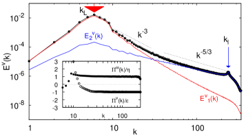
Figure 1: (color online) Average energy spectrum $E_{v}(k)$ (symbols). $E^{v}_{1,2}(k)$ labels the energy spectra associated with the auxiliary velocities $\bm{v}_{1,2}$ and suggests a direct (inverse) cascade for $\bm{v}_{1}$ ($\bm{v}_{2}$), see text. Arrows mark the forcing bands at $k_{L}\!\approx\!7$ and $k_{\ell}\!\approx\!240$. Dotted lines show the slopes $-3$ and $-5/3$. Inset: energy $\Pi^{v}(k)$ and enstrophy $\Pi^{\omega}(k)$ fluxes normalized by their average values ($\epsilon$ and $\eta$, resp.). DNS of Eqs. (1-3) were done with a standard $2/3$-dealiased, pseudospectal method with $1024^{2}$ collocation points.

In Ref. Gage1986 , to explain the observed universality of atmospheric spectra, it was conjectured that the two sources may not be independent. However, large and small scale excitations originate from different physical processes VallisBook characterized by separate timescales (small-scale convection being faster), bearing their independence. Within the independent-source model, spectral universality can be ascribed to that of the inverse-cascade Boffetta2000 . In FolkmarLarsen1982 ; Gage1986 it was also hypothesized that oppositely directed cascades could not coexist without a sink between the forcing scales. Lilly Lilly1989 , using closure theories, showed that there is no need of such sink. Maltrud and Vallis Maltrud1991 made, as far as we know, the unique numerical study of Eq. (1), providing evidence of two overlapping cascades. This is confirmed by Fig. 1 which shows that the energy spectrum $E_{v}(k)$ displays the basic features of the atmospheric one. Moreover, enstrophy $\Pi^{\omega}(k)$ and energy $\Pi^{v}(k)$ fluxes are constant with opposite signs ($\Pi^{\omega}(k)>0$ and $\Pi^{v}(k)<0$) meaning that direct enstrophy and inverse energy cascades superimpose, apparently undisturbed, in the same range $[k_{L}:k_{\ell}]$. We show below that, remarkably, the superposition is realized maintaining non-trivial correlations between the degrees of freedom associated with the two cascades.

To scrutinize this superposition we propose a decomposition able to disentangle the two cascades, by evolving in parallel with Eq. (1) two auxiliary equations

$${}\partial_{t}\omega_{{}_{L}}+\bm{v}\cdot\bm{\nabla}\omega_{{}_{L}}\!\!=-\nu_{p}(-\Delta)^{p}\omega_{{}_{L}}\!\!-\alpha_{q}(-\Delta)^{-q}\omega_{{}_{L}}\!\!+f_{{}_{L}}$$ (2)

$${}\partial_{t}\omega_{\ell}\,+\bm{v}\cdot\bm{\nabla}\omega_{\ell}\!=-\nu_{p}(-\Delta)^{p}\omega_{\ell}-\alpha_{q}(-\Delta)^{-q}\omega_{\ell}\!+f_{\ell}\,,$$ (3)

where $\bm{v}$ is the same as in Eq. (1). Since $f_{L}$ and $f_{\ell}$ in (2-3) are the same realizations of the forcings in (1), $\omega_{{{}_{L}},\ell}$ are two “active” pseudo-scalar fields Celani2002 , such that $\omega\!=\!\omega_{{}_{L}}\!+\!\omega_{\ell}$ and $\bm{v}\!=\!\bm{v}_{{}_{L}}\!+\!\bm{v}_{\ell}$ nota1 , with $\bm{v}_{{{}_{L}},\ell}\!=\!\bm{\nabla}^{\perp}\psi_{{{}_{L}},\ell}$ ($\Delta\psi_{{{}_{L}},\ell}=-\omega_{{}_{L},\ell}$) incompressible. In the sequel, we adopt the notation $\bm{v}\!\equiv\!\bm{v}_{0}$, $\omega\!\equiv\!\omega_{0}$, $\bm{v}_{{{}_{L}},\ell}\!\equiv\!\bm{v}_{1,2}$ and $\omega_{{{}_{L}},\ell}\!\equiv\!\omega_{1,2}$.

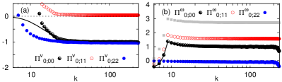
Figure 2: (color online) Dynamical fluxes of (a) energy $\Pi^{v}_{0;jj}(k)$ and (b) enstrophy $\Pi^{\omega}_{0;jj}(k)$ (defined in nota2 ). Grey symbols in (b) refer to passive scalar flux $\Pi^{\theta}$, see text (Cfr. Eq.(10)). The solid curves show energy and enstrophy fluxes obtained by integrating (2) with $f_{L}=0$ (a) or $f_{\ell}=0$ (b), their superposition to $\Pi^{v}_{0;00}$ and $\Pi^{\omega}_{0;00}$, resp. further demonstrates the cascades overlap when both forcings are present. Notice that $\Pi^{v}_{0;22}\approx\Pi^{v}_{0;00}<0$ and $\Pi^{v}_{0;11}\approx 0$ making evident that $\bm{v}_{2}$ are the degrees of freedom associated with the inverse cascade. Similar considerations apply to vorticity, though $\Pi^{\omega}_{0;11}>\Pi^{\omega}_{0;00}$, which will be discussed later in relation to Fig. 4.

The behavior of the energy spectra (Fig. 1) and the fluxes (Fig. 2) associated with the auxiliary fields suggest the identification of the components $\bm{v}_{1,2}$ as the carriers of the degrees of freedom mainly associated with, respectively, the direct and the inverse cascade. This observation can be substantiated by means of the Kármán-Howarth-Monin (KHM) equation Frisch1995 $(\partial_{t}+\alpha_{q}(-\Delta)^{-q})C_{jk}(\bm{r},t)+\mathcal{E}_{jk}(\bm{r},t)-F_{jk}(\bm{r},t)=\frac{1}{2}\partial_{\alpha}\mathcal{S}_{0jk}^{\alpha\beta\beta}(\bm{r},t)$ (as customary, we assumed translation, rotation and parity invariance). The KHM equation links the $3^{rd}$ order structure-tensor,

$$\mathcal{S}_{ijk}^{\alpha_{i}\alpha_{j}\alpha_{k}}(\bm{r})=\prec\!\!\delta v_{i}^{\alpha_{i}}(\bm{r})\delta v_{j}^{\alpha_{j}}(\bm{r})\delta v_{k}^{\alpha_{k}}(\bm{r})\!\!\succ$$ (4)

($\delta\bm{v}_{i}(\bm{r})\!\equiv\!\bm{v}_{i}(\bm{r},t)-\bm{v}_{i}(\bm{0},t)$), to the correlation functions of velocities ($C_{jk}(\bm{r},t)\!=\prec\!\!\bm{v}_{j}(\bm{r},t)\cdot\bm{v}_{k}(\bm{0},t)\!\!\succ$) and forcings ($F_{jk}(\bm{r})\!=\prec\!\!f_{j}(\bm{r},t)f_{k}(\bm{0},t)\!\!\succ$) and to the dissipative terms $\mathcal{E}_{jk}(\bm{r},t)=2\nu_{p}\prec\!\nabla_{\alpha}^{p}v^{\beta}_{j}(\bm{r},t)\nabla_{\alpha}^{p}v^{\beta}_{k}(\bm{0},t)\!\succ$. Kraichnan’s theory is equivalent to the following three hypotheses Be99 : existence of steady state for Galilean invariant statistical indicators; smoothness at finite viscosity; absence of velocity dissipative anomaly. Using these hypotheses, a careful analysis along the lines of Be99 ; Lindborg1999 ; Mazzino2007 justifies in the range $\ell\ll r\ll L$, the expansion

$$\mathcal{S}_{ijk}^{\alpha_{i}\alpha_{j}\alpha_{k}}(\bm{r})={\mbox{$\sum_{n=0,1}$}}r^{2\,n}P_{ijk}\left\{r^{\alpha_{i}}A_{\left\{i[jk]:n\right\}}\delta^{\alpha_{j}\alpha_{k}}\right\}$$ (5)

$$-\,{\scriptstyle\frac{2}{3}}\,P_{ijk}\left\{A_{\left\{i[jk]:n\right\}}\right\}\,r^{\alpha_{i}}r^{\alpha_{j}}r^{\alpha_{k}}+o(r^{3})\,,$$

with shorthand notation for summation over cyclic permutations, $P_{ijk}\left\{O_{ijk}\right\}\!\equiv\!O_{ijk}\!+\!O_{jki}\!+\!O_{kij}$ for any $O$. Eq. (5) holds true strictly for $i=0$ in the ideal limit of infinite volume at vanishing hypofriction $(\alpha_{q}=0)$, with, furthermore, the explicit prediction for the coefficients:

$${}A_{\left\{0[jk]:0\right\}}+P_{0jk}\left\{A_{\left\{0[jk]:0\right\}}\right\}=2\,\epsilon\,(\delta_{j0}+\delta_{j2})(\delta_{k0}+\delta_{k2})$$ (6)

$${}A_{\left\{0[jk]:1\right\}}+{\scriptstyle\frac{1}{3}}P_{0jk}\left\{\!A_{\left\{0[jk]:1\right\}}\!\right\}={\scriptstyle\frac{1}{4}}\eta\,(\delta_{j0}+\delta_{j1})(\delta_{k0}+\delta_{k1}).$$ (7)

Out of the ideal limit, the constants $A_{\left\{i[jk]:n\right\}}=A_{\left\{i[kj]:n\right\}}$ depend on the full statistics of the solution of Eqs. (1-3). Moreover, for $i=1,2$, no dynamical constraints can be imposed to fix the constants $A_{\left\{i[jk]:\{0,1\}\right\}}$, however the expansion (5) can still be justified using parity invariance and the incompressibility of the fields $\bm{v}_{i}$. The quantities $\mathcal{S}_{0jk}$ are thus associated with dynamical fluxes, while $\mathcal{S}_{1jk}$ and $\mathcal{S}_{2jk}$ only provide statistical information, and will be dubbed “statistical” fluxes. Eqs. (5-7) recover the $3^{rd}$-order longitudinal structure function derived in Ref. Lindborg1999 :

$${}S_{000}^{L}(r)\!\equiv\!r_{\alpha_{1}}r_{\alpha_{2}}r_{\alpha_{3}}\mathcal{S}_{000}^{\alpha_{1}\alpha_{2}\alpha_{3}}(r)/r^{3}={\scriptstyle\frac{3}{2}}\epsilon\,r+{\scriptstyle\frac{1}{8}}\eta\,r^{3}\,,$$ (8)

which is numerically very well satisfied (Fig. 3a). Interestingly, other quantities deviate from the ideal limit prediction (e.g $S_{012}^{{L}}(r)\!=\!0$ is not reproduced by data, see Fig. 3a). As discussed below, similar issues are present for $3^{rd}$-order quantities associated with $\omega_{i}$ ($i=0,1,2$). The deviations from ideal-limit predictions should be ascribed to the finiteness of the simulation domain, where the presence of hypofriction stymies the derivation of neat relations such as (7). The $A_{\left\{\dots:1\right\}}$’s become coupled to the infra-red component of the kinetic energy hinting at a more non-local and less universal behavior of the enstrophy cascade. This fact relates to non-trivial correlations existing between the degrees of freedom associated with the two cascades. The importance of such correlations can be quantified by comparing the “statistical” fluxes $\Pi^{v,\omega}_{1;jj}(k)$ and $\Pi^{v,\omega}_{2;jj}(k)$ (with $j=0,1,2$), defined in nota2 , with the “dynamical” fluxes $\Pi^{v,\omega}_{0;jj}$’s (for $j=0,1,2)$. As shown in Fig. 4, two phenomena stand out.

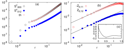
Figure 3: (color online) $3^{rd}$ structure functions: (a) for velocity $S_{000}^{L}(r)$ compared with the prediction (8) (solid red line) and $S_{012}^{L}(r)$; (b) for vorticity $-Z_{0;11}(r)\!\equiv\!-\bm{r}\cdot\mathcal{Z}_{0;11}(\bm{r})/r$ and $Z_{0;12}(r)$, the black lines show linear behavior in $r$. The negative linear behavior of $Z_{0;11}(r)$ links to the direct cascade of $\prec\!\omega_{1}^{2}\!\succ$; (c) $\mathcal{C}^{\omega}_{12}(r)=\prec\!\omega_{1}(0)\omega_{2}(\bm{r})\!\succ$ vs $r$. The behaviors of $Z_{0;12}(r)$ (which should vanish in the ideal limit) and of $\mathcal{C}^{\omega}_{12}(r)$ are evidences of the sensitivity of directly cascading degrees of freedom to the hypofriction, see text (Cfr. Eq. (Nonlinear superposition of direct and inverse cascades in two-dimensional turbulence forced at large and small scales)).

Whilst $\Pi^{v}_{0;00}\simeq\Pi^{v}_{0;22}<0$ (Fig. 2a) validates the identification of $\bm{v}_{2}$ as the degrees of freedom associated with the inverse cascade, the left panels of Fig. 4 show that $\Pi^{v}_{1;00}<\!0$ ($\Pi^{v}_{1;22}<\!0$) with intensity comparable to that of $\Pi^{v}_{2;00}$ ($\Pi^{v}_{2;22}$) and thus indicates that $\bm{v}_{1}$ contributes to the inverse cascade of the total field $\bm{v}_{0}$. This may appear, at first glance, surprising in consideration of the observed absence of flux of kinetic energy of $\bm{v}_{1}$ ($\Pi^{v}_{i;11}\simeq\!0$ for any $i$). The non-intuitive and, possibly, non-universal behavior of the statistical energy fluxes $\Pi^{v}_{i;jj}$ ($i\!=\!1,2$) is, however, a consequence of their dependence on the full statistics. Similar considerations apply to enstrophy fluxes, with the roles of $\bm{v}_{1}$ and $\bm{v}_{2}$ exchanged (Fig. 4 right).

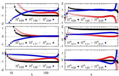
Figure 4: (color online) Fluxes of energy and enstrophy defined in nota2 : (Left) energy fluxes $\Pi^{v}_{i;jj}$ of $\bm{v}_{j}$ ($j=0,1,2$ from top to bottom) due to the transport by $\bm{v}_{i}$ ($i=0$ black semifilled circles, $i=1$ red empty circles, $i=2$ blue filled circles); (Right) Enstrophy fluxes $\Pi^{\omega}_{i;jj}$: panels, symbols and colors follow the same convention of Left panel.

The second phenomenon appertains to the relative intensity of enstrophy fluxes. The ideal-limit energy-balance predictions (6-7) suggest $\Pi_{0;00}^{\omega}\simeq\Pi_{0;11}^{\omega}\,>\,0$ with $\Pi_{0;22}^{\omega}\simeq 0$. The right panels of Fig. 4 confirm the latter prediction coherently with the interpretation of $\bm{v}_{2}$ as the carrier of the inverse cascade degrees of freedom. They also show that the “dynamical” enstrophy flux $\Pi_{0;11}^{\omega}$ is significantly enhanced with respect to $\Pi_{0;00}^{\omega}$ (see also Fig. 2b). The phenomenon can be regarded as a consequence of the alleged fact that the main contribution to $\bm{v}_{1}$ comes from the degrees of freedom of $\bm{v}_{0}$ undergoing the direct cascade and of the stronger sensitivity of this latter to non-local effects. In order to substantiate the claim we inspected the equations governing the correlation functions $\mathcal{C}^{\omega}_{ij}(\bm{r})=\prec\!\!\omega_{i}(0)\omega_{j}(\bm{r})\!\!\succ$. From the energy balance in the presence of hypofriction together with the assumption of inverse cascading $\bm{v}_{2}$ (i.e. $\Pi^{\omega}_{0;22}\sim 0$ with $\alpha_{q}\,(-\Delta)^{q}\mathcal{C}^{\omega}_{22}(\bm{0})=F_{\ell}=\prec\!f_{\ell}^{2}\!\succ$) we derived that

$${}\Pi^{\omega}_{0;11}-\Pi^{\omega}_{0;00}={\scriptstyle\frac{1}{2}}\alpha_{q}\,(-\Delta)^{q}(\mathcal{C}^{\omega}_{00}-\mathcal{C}^{\omega}_{11})(\bm{0})-F_{\ell}$$

$${\hskip 8.5359pt}+O(k\,L)^{\gamma}\simeq\alpha_{q}\,(-\Delta)^{q}\mathcal{C}^{\omega}_{12}(\bm{0})+O(k\,L)^{\gamma}$$ (9)

for some $\gamma>\!0$, as enstrophy is bounded Be99 . Eq. (Nonlinear superposition of direct and inverse cascades in two-dimensional turbulence forced at large and small scales) evinces the non-local nature of the enstrophy transfer. Its positive value implies that the correlation $\mathcal{C}^{\omega}_{12}(r)$ must be also positive in the inertial range, as confirmed in Fig. 3c. In terms of the vorticity structure functions $\bm{\mathcal{Z}}_{i;jk}(\bm{r})\equiv\prec\!\delta\bm{v}_{i}(r)\delta\omega_{j}(\bm{r})\delta\omega_{k}(\bm{r})\!\succ$, Eq. (Nonlinear superposition of direct and inverse cascades in two-dimensional turbulence forced at large and small scales) translates into $Z_{0;12}(r)=\bm{r}\cdot\bm{\mathcal{Z}}_{0;12}(r)/r>0$ with linear dependence on $r$ (as shown in Fig. 3b), while it should be $0$ in the ideal limit. To further elucidate the enhancement of $\Pi^{\omega}_{0;11}$ with respect to $\Pi^{\omega}_{0;00}$, it is instructive to liken the ultra-violet behavior of the vorticity $\omega_{1}$ to that of a passive scalar $\theta$ evolving in the same velocity field, as in Ref. Boffetta2002 :

$$\partial_{t}\theta+\bm{v}\cdot\bm{\nabla}\theta\!\!=-\nu_{p}(-\Delta)^{p}\theta\!\!-\alpha_{q}(-\Delta)^{-q}\theta\!\!+f^{\prime}_{{}_{L}}$$ (10)

Here, the large-scale forcing $f^{\prime}_{{}_{L}}$ has the same statistics of that used in (2) but with independent realizations, making $\theta$ a passive scalar Celani2002 . Flow incompressibility brings about a scalar energy $\prec\!\theta^{2}\!\succ\!\!/2$ cascade to smaller scales, and similarly to (Nonlinear superposition of direct and inverse cascades in two-dimensional turbulence forced at large and small scales), by energy balance, we have

$${}\Pi^{\theta}\!-\!\Pi_{0;00}^{\omega}\simeq\alpha_{q}(-\partial_{\bm{x}}^{-2})^{q}(\mathcal{C}_{00}^{\omega}-\mathcal{C}^{\theta})(\bm{0})/2+O(k\,L)^{\gamma^{\prime}}$$ (11)

for some positive $\gamma^{\prime}$, where $\mathcal{C}^{\theta}(\bm{r})=\prec\!\theta(\bm{r},t)\theta(\bm{0},t)\!\succ$. We expect the difference in (11) to be positive as the infra-red content of $\mathcal{C}_{00}^{\omega}$ is “fattened” by the inverse energy transfer at $k<k_{L}$. As shown in Fig. 2b, the comparison between the passive scalar energy flux, $\Pi^{\theta}$, with the enstrophy flux, $\Pi^{\omega}_{0;00}$ validates this prediction. The inference is that the same phenomenon underlies the positive sign of (Nonlinear superposition of direct and inverse cascades in two-dimensional turbulence forced at large and small scales).

Summarizing, we showed that 2d-turbulence sustained by a large and a small scale forcing gives rise in between the sources to an inertial range where a direct and an inverse cascade co-exist and overlap. We also showed that there exists a natural decomposition of the Navier–Stokes field compartmentalizing the degrees of freedom associated with the direct and inverse cascade in two auxiliary velocity fields, obtained considering a single large and small scale source, respectively. Although these auxiliary fields satisfy energy balance relations as if they were independent, actually they are not and exhibit non-trivial correlations pinpointed by the inspection of third order statistics of “statistical” objects, evading the energy balance relations. In contrast to the settings used here, realistic forcings in the atmosphere should be time-correlated, with the large-scale excitation being slower than the small-scale one. Provided the forcings are independent with separate spatial and temporal scale the picture presented here should remain essentially unaltered. However, a slow large-scale forcing may induce coherent motions that, as argued in Ref. Xia2008 , can change the sign of the (total) energy flux and thus mask the inverse cascade process, which may explain observations Cho2001 .

We conclude with a theoretical remark. The decomposition in terms of auxiliary velocity fields here proposed can be straightforwardly generalized to $2d$ Navier-Stokes equations with an energy input distributed over different scales. In this perspective, the cascade overlap of the two sources model, here investigated, evinces the physical mechanism for why Kraichnan theory applies also in the presence of power-law sources and, consequently, for the inability of renormalization group approach to correctly predict Navier-Stokes energy spectra Mazzino2007 , even in what may seem a priori a perturbative regime.

References

• (1) U. Frisch, Turbulence: the legacy of AN Kolmogorov (Cambridge University Press, 1995)
• (2) R. H. Kraichnan, Phys. Fluids 10, 1417 (1967)
• (3) R. Kraichnan, J. Fluid Mech. 47, 525 (1971)
• (4) G. Boffetta, A. Celani, and M. Vergassola, Phys. Rev. E 61, 29 (2000)
• (5) G. Boffetta and S. Musacchio, Phys. Rev. E 82, 016307 (2010)
• (6) L. Smith, J. Chasnov, and F. Waleffe, Phys. Rev. Lett. 77, 2467 (1996)
• (7) A. Celani, S. Musacchio, and D. Vincenzi, Phys. Rev. Lett. 104, 184506 (2010)
• (8) H. Xia, D. Byrne, G. Falkovich, and M. Shats, Nature Phys. 7, 321 (2011)
• (9) G. Nastrom, K. Gage, and W. Jasperson, Nature 310, 36 (1984)
• (10) E. Lindborg, J. Fluid Mech. 388, 259 (1999)
• (11) G. Vallis, Atmospheric and oceanic fluid dynamics: fundamentals and large-scale circulation (Cambridge University Press, 2006)
• (12) J. Y. N. Cho and E. Lindborg, J. Geophys. Res 106, 223 (2001)
• (13) K. Gage, J. Atmos. Sci. 36, 1950 (1979)
• (14) M. Folkmar Larsen, M. Kelley, and K. Gage, J. Atmos. Sci. 39, 1035 (1982)
• (15) D. Lilly, J. Atmos. Sci. 46, 2026 (1989)
• (16) K. Gage and G. Nastrom, J. Atmos. Sci. 43, 729 (1986)
• (17) E. Dewan, Science 204, 832 (1979)
• (18) T. VanZandt, Geophys. Res. Lett. 9, 575 (1982)
• (19) H. Xia, H. Punzmann, G. Falkovich, and M. Shats, Phys. Rev. Lett. 101, 194504 (2008)
• (20) L. Smith and V. Yakhot, J. Fluid Mech. 274, 115 (1994)
• (21) E. Lindborg, J. Fluid Mech. 550, 207 (2006)
• (22) Y. Kitamura and Y. Matsuda, Geophys. Res. Lett. 33, L05809 (2006)
• (23) R. Tulloch and K. Smith, Proc. Natl. Acad. Sci. 103, 14690 (2006)
• (24) M. Maltrud and G. Vallis, J. Fluid Mech. 228, 321 (1991)
• (25) A. Celani, M. Cencini, A. Mazzino, and M. Vergassola, Phys. Rev. Lett. 89, 234502 (2002); New J. Phys. 6, 72 (2004).
• (26) In simulations it is enough to integrate Eqs.(1) and (2) and obtain $\omega_{\ell}$ by subtraction.
• (27) Πi;jjv(k)=\ilimits@q>kd2q(2\tmspace+.1667emπ)2\ilimits@2𝑑𝒓\tmspace+.1667emeı𝒒𝒓\tmspace+.1667emα𝒮ijjαββ(𝒓)subscriptsuperscriptΠ𝑣𝑖𝑗𝑗𝑘subscript\ilimits@𝑞𝑘superscript𝑑2𝑞superscript2\tmspace.1667𝑒𝑚𝜋2subscript\ilimits@superscript2differential-d𝒓\tmspace.1667𝑒𝑚superscript𝑒italic-ı𝒒𝒓\tmspace.1667𝑒𝑚subscript𝛼superscriptsubscript𝒮𝑖𝑗𝑗𝛼𝛽𝛽𝒓\Pi^{v}_{i;jj}(k)=\intop\ilimits@_{q>k}\frac{d^{2}q}{(2\tmspace+{.1667em}\pi)^{2}}\intop\ilimits@_{\mathbb{R}^{2}}d\bm{r}\tmspace+{.1667em}e^{-\imath\bm{q}\cdot\bm{r}}\tmspace+{.1667em}\nabla_{\alpha}\mathcal{S}_{ijj}^{\alpha\beta\beta}(\bm{r}), and Πi;jjω(k)=\ilimits@q>kd2q(2\tmspace+.1667emπ)2\ilimits@2𝑑𝒓x\tmspace+.1667emeı𝒒𝒓\tmspace+.1667emα(Δ)𝒮ijjαββ(𝒓)subscriptsuperscriptΠ𝜔𝑖𝑗𝑗𝑘subscript\ilimits@𝑞𝑘superscript𝑑2𝑞superscript2\tmspace.1667𝑒𝑚𝜋2subscript\ilimits@superscript2differential-d𝒓𝑥\tmspace.1667𝑒𝑚superscript𝑒italic-ı𝒒𝒓\tmspace.1667𝑒𝑚subscript𝛼Δsuperscriptsubscript𝒮𝑖𝑗𝑗𝛼𝛽𝛽𝒓\Pi^{\omega}_{i;jj}(k)=\intop\ilimits@_{q>k}\frac{d^{2}q}{(2\tmspace+{.1667em}\pi)^{2}}\intop\ilimits@_{\mathbb{R}^{2}}d\bm{r}x\tmspace+{.1667em}e^{-\imath\bm{q}\cdot\bm{r}}\tmspace+{.1667em}\nabla_{\alpha}(-\Delta)\mathcal{S}_{ijj}^{\alpha\beta\beta}(\bm{r}), with Einstein convention on repeated Greek indexes. Note that, by construction, $\Pi^{v,\omega}_{1;jj}\!+\!\Pi^{v,\omega}_{2;jj}\!\!=\!\Pi^{v,\omega}_{0;jj}$ for any $j$
• (28) D. Bernard, Phys. Rev. E 60, 6184 (1999); Europhys. Lett. 50, 333 (2000)
• (29) G. Boffetta, A. Celani, S. Musacchio, and M. Vergassola, Phys. Rev. E 66, 026304 (2002)
• (30) A. Mazzino, P. Muratore-Ginanneschi, and S. Musacchio, Phys. Rev. Lett. 99, 144502 (2007); JSTAT, P10012 (2009).