Measuring the Fourth Generation $b\to s$ Quadrangle at the LHC

Abstract

We show that simultaneous precision measurements of the $CP$-violating phase in time-dependent $B_{s}\to J/\psi\phi$ study and the $B_{s}\to\mu^{+}\mu^{-}$ rate, together with measuring $m_{t^{\prime}}$ by direct search at the LHC, would determine $V_{t^{\prime}s}^{*}V_{t^{\prime}b}$ and therefore the $b\to s$ quadrangle in the four-generation standard model. The forward–backward asymmetry in $B\to K^{*}\ell^{+}\ell^{-}$ provides further discrimination.

PACS numbers

14.65.Jk 12.15.Hh 11.30.Er 13.20.He

I INTRODUCTION

Much like the completion of the three-generation “$b\to d$ triangle” in 2001 by the B factories, we may be at the dawn of measuring the “$b\to s$ quadrangle” at the LHC, if a fourth generation of quarks should exist.

Measurement of the time-dependent $CP$-violating (CPV) phase $\sin 2\beta/\phi_{1}$ in $B_{d}\to J/\psi K^{0}$ decays by the BaBar and Belle experiments confirmed PDG the Kobayashi–Maskawa Kobayashi:1973fv mechanism of the standard model with three generations of quarks (SM3). Here, $\sin 2\beta=\sin 2\phi_{1}\equiv\sin 2\Phi_{B_{d}}$ is the CPV phase of the $\bar{B}_{d}\to B_{d}$ mixing amplitude. With the continuous run of the Large Hadron Collider (LHC) throughout 2011-2012, the LHCb experiment will measure $\sin 2\Phi_{B_{s}}$, the CPV phase of $\bar{B}_{s}\to B_{s}$ mixing, via time-dependent study of $B_{s}\to J/\psi\phi$ and similar decays. We point out that, together with the measurement of $B_{s}\to\mu^{+}\mu^{-}$ rate, which is accessible not only by LHCb, but by the CMS experiment (and eventually, ATLAS) as well, combined with the direct search program of fourth-generation quarks, one may determine the Cabibbo–Kobayashi–Maskawa (CKM) mixing matrix element Kobayashi:1973fv ; Cabibbo:1963yz ; Glashow:1970gm product $V_{t^{\prime}s}V_{t^{\prime}b}^{*}$, thereby complete the SM4 quadrangle of

$$V_{us}V_{ub}^{*}+V_{cs}V_{cb}^{*}+V_{ts}V_{tb}^{*}+V_{t^{\prime}s}V_{t^{\prime}b}^{*}=0.$$ (1)

Much progress has been made in summer 2011 on the above, so let us retrace how we reached the present.

Interest in the fourth generation renewed with the “$B\to K\pi$ direct CPV (DCPV) difference” puzzle: DCPV in $B^{+}\to K^{+}\pi^{0}$ and $B^{0}\to K^{+}\pi^{-}$ appeared opposite in sign BelleNature ; PDG , even though they proceed by the same spectator diagrams. The effect could be due to HNS the nondecoupling of the heavy SM4 $t^{\prime}$ quark in the $bsZ$ penguin, which brings in a new CPV phase in $V_{t^{\prime}s}^{*}V_{t^{\prime}b}$. But hadronic effects make the $B\to K\pi$ DCPV measurements less amenable to interpretation.

However, an SM4 effect in the $b\to s$ $Z$-penguin loop should give a correlated effect in the $b\bar{s}\to s\bar{b}$ box diagram, making $\sin 2\Phi_{B_{s}}$ large and negative HNS ; Hou:2005yb , in contrast with $-0.04$ in SM3. After the 2006 measurement PDG of $B_{s}$ mixing, i.e., $\Delta m_{B_{s}}$, by the CDF experiment at the Tevatron, the “prediction” was strengthened Hou:2006mx to “$\sin 2\Phi_{B_{s}}=-0.5$ to $-0.7$ for $m_{t^{\prime}}=300$ GeV.” Interestingly, by 2008, both the CDF and D0 experiments reported PDG hints for negative $\sin 2\Phi_{B_{s}}$ (called respectively $-\sin 2\beta_{s}$ and $\sin\phi_{s}$). Although weakening in 2010, the measurement LHCb10 by LHCb using just the 2010 data of 36 pb^-1 showed a $\sin\phi_{s}$ that deviated from SM3 by $1.2\sigma$, i.e., in same direction as CDF and D0! So, there was much anticipation for LHCb to unveil their result with 10 times the data. To one’s surprise, however, analyzing 0.34 fb^-1 data, the LHCb experiment found Raven

$$\phi_{s}\equiv 2\Phi_{B_{s}}=0.03\pm 0.16\pm 0.07,\ \ \ {\rm(LHCb\ 0.34\ fb}^{-1})$$ (2)

which is consistent with zero (hence SM3). In fact, $B_{s}\to J/\psi\phi$ alone gave $0.13\pm 0.18\pm 0.07$, while Eq. (2) is the combined result with $B_{s}\to J/\psi f_{0}(980)$.

There was another development that aroused the interest in the fourth generation in the past few years, namely the realization Kribs:2007nz ; Holdom:2009rf in 2007 that electroweak precision tests did not firmly rule out a fourth generation, but rather indicated that the $t^{\prime}$, $b^{\prime}$ quarks be heavy, split in mass — but not by too much — while the Higgs mass bound would loosen. The direct search for $t^{\prime}$ and $b^{\prime}$ at the Tevatron had in any case been ongoing. At the LHC, the limit Chatrchyan:2011em of $m_{b^{\prime}}>361$ GeV (95% C.L.) was reached with 2010 data alone, and became 495 (450) GeV for $b^{\prime}$ ($t^{\prime}$) by DeRoeck summer 2011. We are already at the doorstep of the unitarity bound (UB) of 500–550 GeV Chanowitz:1978uj .

It is difficult to enhance $B_{s}\to\mu^{+}\mu^{-}$ in SM4 by more than a factor of 2, because it is constrained by $B\to X_{s}\ell^{+}\ell^{-}$, which is consistent with SM3 in rate. Hence, this mode appeared less relevant for SM4, until recently. Based on 2010 data, the competitive limit Aaij:2011rj by LHCb was already within 20 times the SM3 expectation of $3.2\times 10^{-9}$ Buras:2010pi . Since 2010, the progress is significant, both at the Tevatron and the LHC (see Note Added), and a measurement of $B_{s}\to\mu^{+}\mu^{-}$ at the SM3 level now seems possible with 2011-2012 LHC data. With the signal of two charged tracks from a displaced vertex, the CMS experiment has demonstrated its competitiveness, in part due to an advantage in luminosity. The combined result comboBsmumu of LHCb and CMS gives

$${\cal B}(B_{s}\to\mu^{+}\mu^{-})<11\times 10^{-9},\ \ {\rm(LHCb+CMS,\,2011)}$$ (3)

at 95% CL, which is only 3.5 times the SM3 level.

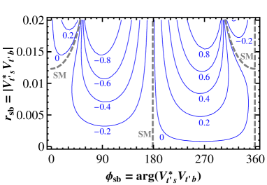
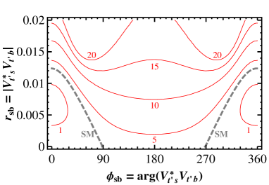
Figure 1: Contours of (a) $\sin 2\Phi_{B_{s}}$, (b) $10^{9}\times{\cal B}(B_{s}\to\mu^{+}\mu^{-})$ in $\arg V_{t^{\prime}s}^{*}V_{t^{\prime}b}$–$|V_{t^{\prime}s}^{*}V_{t^{\prime}b}|$ plane for $m_{t^{\prime}}=550$ GeV.

While $B_{s}\to\mu^{+}\mu^{-}$ has been considered in recent SM4 studies Buras:2010pi ; Soni:2010xh ; Eberhardt:2010bm ; Golowich:2011cx , what we point out is that, together with the measurements of $\sin 2\Phi_{B_{s}}$ and $m_{t^{\prime}}$, the CKM element product $V_{t^{\prime}s}^{*}V_{t^{\prime}b}$ can be determined. Since $V_{us}^{*}V_{ub}$ and $V_{cs}^{*}V_{cb}$ are known from tree processes, a measurement of $V_{t^{\prime}s}^{*}V_{t^{\prime}b}$ would already complete the $b\to s$ quadrangle of Eq. (1), assuming that one has only SM4 and no other new physics. This quadrangle could be relevant for Hou:2008xd the baryon asymmetry of our Universe (BAU). We will discuss the issue of the Higgs boson at the end.

II Impact of $\sin 2\Phi_{B_{s}}$ and $B_{s}\to\mu^{+}\mu^{-}$

The $\bar{B}_{s}$–$B_{s}$ mixing amplitude is well-known,

$$M_{12}^{s} = \frac{G_{F}^{2}M_{W}^{2}}{12\pi^{2}}m_{B_{s}}f_{B_{s}}^{2}\hat{B}_{B_{s}}\eta_{B}\Bigl{[}\left(\lambda_{t}^{\rm\scriptsize SM}\right)^{2}S_{0}(t,t)$$ (4)

$$\ \ \ \ \ \ \ \;\;+2\lambda_{t}^{\rm\scriptsize SM}\lambda_{t^{\prime}}\Delta S_{0}^{(1)}+\lambda_{t^{\prime}}^{2}\Delta S_{0}^{(2)}\Bigr{]},$$

where $\lambda_{q}\equiv V_{qs}^{*}V_{qb}$ hence $-\lambda_{t}^{\rm\scriptsize SM}=\lambda_{c}+\lambda_{u}$, and we have approximated by factoring out a common short distance QCD factor $\eta_{B}$. With $S_{0}$ and $\Delta S_{0}^{(i)}$ as defined in Ref. Hou:2006mx , Eq. (4) manifestly respects the Glashow-Iliopoulos-Maiani (GIM) mechanism Glashow:1970gm .

The mass difference $\Delta m_{B_{s}}\equiv 2|M_{12}^{s}|$ depends on the hadronic parameter $f_{B_{s}}^{2}\hat{B}_{B_{s}}$, hence it is not useful for extracting short distance information. However, defining $\Delta_{12}^{s}=[\;\ldots\;]$ in Eq. (4), the CPV phase

$$2\Phi_{B_{s}}\equiv\arg M_{12}^{s}=\arg\Delta_{12}^{s},$$ (5)

depends only on $m_{t^{\prime}}$ and $\lambda_{t^{\prime}}=V_{t^{\prime}s}^{*}V_{t^{\prime}b}$. Note that $\lambda_{t}^{\rm\scriptsize SM}\cong-0.04-V_{us}^{*}V_{ub}$, and we will take the current best fit value for $V_{us}^{*}V_{ub}$ from PDG PDG . Note that $V_{us}^{*}V_{ub}$ can be directly measured via tree processes at LHCb.

We plot, in Fig. 1(a), the contours for $\sin 2\Phi_{B_{s}}$ in the $\phi_{sb}\equiv\arg V_{t^{\prime}s}^{*}V_{t^{\prime}b}$, $r_{sb}\equiv|V_{t^{\prime}s}^{*}V_{t^{\prime}b}|$ plane for $m_{t^{\prime}}=550$ GeV. This $m_{t^{\prime}}$ value is chosen because 500 GeV is almost ruled out, while going beyond 550 GeV, one is no longer sure of the numerical accuracy of Eq. (4). That is, above the UB, the perturbative computation of the functions $\Delta S_{0}^{(i)}$ would no longer be valid. However, some form like Eq. (4) should continue to hold even above the UB. We have checked that our results do not change qualitatively if we straightforwardly apply $m_{t^{\prime}}=650$ GeV.

At first sight, the $B_{s}\to\mu^{+}\mu^{-}$ decay rate is also proportional to $f_{B_{s}}^{2}$, bringing in large hadronic uncertainties. However, this can largely be mitigated Buras:2003td by taking the ratio with $\Delta m_{B_{s}}/\Delta m_{B_{s}}|^{\rm exp}$, namely

$$\mathcal{B}(B_{s}\to\bar{\mu}\mu)=C\frac{\tau_{B_{s}}\eta_{Y}^{2}}{\hat{B}_{B_{s}}\eta_{B}}\frac{|\lambda_{t}^{\rm\scriptsize SM}Y_{0}(x_{t})+\lambda_{t^{\prime}}\Delta Y_{0}|^{2}}{|\Delta_{12}^{s}|/\Delta m_{B_{s}}|^{\rm exp}},$$ (6)

where $C=3g_{W}^{4}m_{\mu}^{2}/2^{7}\pi^{3}M_{W}^{2}$, and $\eta_{Y}=\eta_{Y}(x_{t})=\eta_{Y}(x_{t^{\prime}})$ is taken. Hadronic dependence is now only in the better-known “bag parameter,” $\hat{B}_{B_{s}}$. Furthermore, stronger $t^{\prime}$ dependence is brought in through the short distance function $|\Delta_{12}^{s}|$ that enters $\Delta m_{B_{s}}$. We plot the contours for ${\cal B}(B_{s}\to\mu^{+}\mu^{-})$ in the $\phi_{sb}$–$r_{sb}$ plane for $m_{t^{\prime}}=550$ in Fig. 1(b).

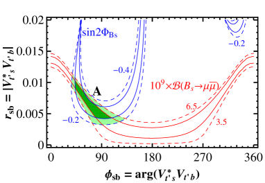
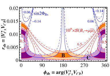
Figure 2: Overlap region for (a) $\sin 2\Phi_{B_{s}}=-0.3\pm 0.1$ and $10^{9}\times{\cal B}(B_{s}\to\mu^{+}\mu^{-})=5.0\pm 1.5$ (Case A), where solid line is for half the error; (b) $\sin 2\Phi_{B_{s}}=-0.04\pm 0.1$, but $10^{9}\times{\cal B}(B_{s}\to\mu^{+}\mu^{-})=5.0\pm 1.5$ (Case B) or $2.0\pm 1.5$ (Case C).

To anticipate the progress with full 2011 data, and towards 2012, we project possible values for $\sin 2\Phi_{B_{s}}$ and ${\cal B}(B_{s}\to\mu^{+}\mu^{-})$. The LHCb result of Eq. (2) is at some odds with earlier results. A study Hou:2010mm of high mass $m_{t^{\prime}}=500$ GeV case considering all relevant data, as compared with $m_{t^{\prime}}=300$ GeV (now ruled out) case studied earlier Hou:2005yb , suggested a smaller $\sin 2\Phi_{B_{s}}$ value of order $-0.3$. This value is still within 2$\sigma$ of Eq. (2). Given the surprise shift from a hint of a large and negative central value prior to 2011, the next update could possibly shift back. Thus, we shall take two possible values

$$\sin 2\Phi_{B_{s}}=-0.3\pm 0.1;\ -0.04\pm 0.1\ \ ({\rm LHCb}>1\;{\rm fb}^{-1})$$ (7)

where the first is more aggressive but reflects the past trend, while the second follows Eq. (2).

An enhanced $\sin 2\Phi_{B_{s}}$ implies the same for $B_{s}\to\mu^{+}\mu^{-}$, so we should entertain the possibility that ${\cal B}(B_{s}\to\mu^{+}\mu^{-})$ is larger than the SM3 value of $3.2\times 10^{-9}$. On the other hand, given that $\sin 2\Phi_{B_{s}}$ is now suitably consistent with SM3, one should consider not only the possibility that ${\cal B}(B_{s}\to\mu^{+}\mu^{-})$ is consistent with SM3, but entertain even the possibility that ${\cal B}(B_{s}\to\mu^{+}\mu^{-})$ might be found to be less than the SM3 expectation. Following the reasoning of Ref. Akeroyd:2011kd for how the luminosity, hence errors, might scale for the combination of LHCb and CMS results, we adopt the two values of

$$10^{9}\,{\cal B}(B_{s}\to\mu^{+}\mu^{-})=5.0\pm 1.5;\ 2.0\pm 1.5\ \ \,({\rm 2012})$$ (8)

to project into 2012. We have chosen two adjacent regions of somewhat enhanced vs somewhat suppressed $B_{s}\to\mu^{+}\mu^{-}$, which contains the SM3 case in intersection. In the following, we will illustrate with the errors as in Eqs. (7) and (8), as well as half the error, anticipating further progress with data.

We illustrate in Fig. 2(a) for $m_{t^{\prime}}=550$ GeV the overlap of the contours for $\sin 2\Phi_{B_{s}}$ and ${\cal B}(B_{s}\to\mu^{+}\mu^{-})$ when both take larger than SM3 values in Eqs. (7) and (8). We denote this as Case A. The light shaded overlap region correspond to the 1$\sigma$ range in Eqs. (7) and (8). Reducing errors by half, one gets the dark shaded area by the overlap of the two sets of solid contours. Roughly speaking, the overlap region extends from $(r_{sb},\;\phi_{sb})\sim(0.011,40^{\circ})$ to $(0.004,130^{\circ})$.

Figure 2(b) shows the cases when $\sin 2\Phi_{B_{s}}=-0.04\pm 0.10$ in Eq. (7), but ${\cal B}(B_{s}\to\mu^{+}\mu^{-})$ is either higher (Case B) or lower (Case C) than SM3 expectations in Eq. (8). The shadings are the same as Fig. 2(a). The two values in Eq. (8) complement each other, as can be seen from Fig. 2(b). Taken together, Cases B+C complement Case A of Fig. 2(a), where both $\sin 2\Phi_{B_{s}}$ and ${\cal B}(B_{s}\to\mu^{+}\mu^{-})$ are on the high side. A remaining Case D is the small region chipped off from Fig. 2(a) that lies between Case A and Cases B+C. We do not discuss this case further, as it can be inferred from Cases A–C.

Inspecting the overlap regions for Cases B and C, both allow large $r_{sb}$ solutions for $|\phi_{sb}|\lesssim 40^{\circ}$, with $r_{sb}$ ranging around 0.013 (0.011) for Case B (C). There is, however, a low $r_{sb}\lesssim 0.004$ overlap region for all $\phi_{sb}$, with Cases B and C complementing each other, with Case B ranging between $90^{\circ}$ to $270^{\circ}$. When $r_{sb}$ is small, in general $\sin 2\Phi_{B_{s}}$ would become close to the SM3 value and become small. The full domain of $\phi_{sb}$ is allowed, which in turn has different implications for ${\cal B}(B_{s}\to\mu^{+}\mu^{-})$. Note that the contour line of ${\cal B}(B_{s}\to\mu^{+}\mu^{-})=3.5\times 10^{-9}$ is very close to the SM3 contour of $3.2\times 10^{-9}$ (the dashed curves in Fig. 1(b)). Thus, to the left of $90^{\circ}$ (and to the right of $270^{\circ}$) for low $r_{sb}$, ${\cal B}(B_{s}\to\mu^{+}\mu^{-})$ is suppressed compared to SM3 (compare Fig. 1(b)), which is precisely Case C. This is a case that still might emerge at the LHC, even when $\sin 2\Phi_{B_{s}}$ is found consistent with SM3. The small $\sin 2\Phi_{B_{s}}$ value can of course turn out to deviate from SM3 when very high precision is reached.

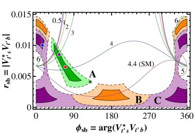
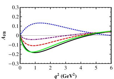
Figure 3: (a) Contours of zero crossing $s_{0}\equiv q^{2}|_{A_{\rm FB}=0}$ in the $\arg V_{t^{\prime}s}^{*}V_{t^{\prime}b}$–$|V_{t^{\prime}s}^{*}V_{t^{\prime}b}|$ plane, overlayed with the overlap regions of Fig. 2 (for $m_{t^{\prime}}=$ 550 GeV); (b) Differential $dA_{\rm FB}/dq^{2}$ vs $q^{2}\equiv m_{\mu^{+}\mu^{-}}^{2}$, where curves from top to bottom (the black solid curve is for SM3) correspond to sample points in overlap regions in (a), indicated by small ellipses, from larger to smaller $r_{sb}$, as explained further in text.

III Utility of $A_{\rm FB}(B^{0}\to K^{*0}\mu^{+}\mu^{-})$

We have focused so far on $\sin 2\Phi_{B_{s}}$ and ${\cal B}(B_{s}\to\mu^{+}\mu^{-})$, the two $B$ physics trump cards in the quest for new physics at the LHC. But a third measurable can be done well by LHCb: the forward-backward asymmetry in $B^{0}\to K^{*0}\mu^{+}\mu^{-}$. Earlier measurements PDG by the B factories, and by CDF, found no indication of a zero crossing. However, the summer 2011 result Patel of LHCb once again turned out in support of SM3. This has implications on the overlap regions of Fig. 2.

The zero crossing point $s_{0}\equiv q^{2}|_{A_{\rm FB}=0}$ is insensitive to form factors, hence an important probe of possible new physics. It has been found generally Buras:2010pi ; Soni:2010xh that, once other flavor and CPV data are taken into account, the variation in $s_{0}$ for SM4 probably cannot be distinguished from SM3 within experimental resolution. But to investigate the power of LHC data alone, we plot in Fig. 3(a) the contours of constant $s_{0}$ in the $\phi_{sb}$–$r_{sb}$ plane for $m_{t^{\prime}}=550$, overlaid with the overlap regions of Fig. 2. We will now show that the consistency of the summer 2011 $A_{\rm FB}(B\to K^{*}\mu^{+}\mu^{-})$ result of LHCb Patel with SM3 rules out the low $\phi_{sb}$, high $r_{sb}$ region, as well as the upper tip of allowed region for Case A.

We take sample points from the overlap regions, illustrated as small ellipses in Fig. 3(a), and plot the corresponding $dA_{\rm FB}/dq^{2}$ vs $q^{2}\equiv m_{\mu^{+}\mu^{-}}^{2}$ in Fig. 3(b), where the black solid curve is for SM3. For the more interesting Case A, i.e., $\sin 2\Phi_{B_{s}}=-0.3\pm 0.1$ and ${\cal B}(B_{s}\to\mu^{+}\mu^{-})=(5.0\pm 1.5)\times 10^{-9}$ both enhanced over SM3 values, we take

$$V_{t^{\prime}s}^{*}V_{t^{\prime}b}\equiv r_{sb}\,e^{i\phi_{sb}}\simeq 0.0065\,e^{i70^{\circ}},$$ (9)

which lies near the center of the allowed region for Case A (third small ellipse from left in Fig. 3(a)), and is close to the $s_{0}\simeq 4$ GeV² contour. This is plotted as the red dashed curve in Fig. 3(b), where we have used the form factor model of Ref. Ball:2004rg within QCD factorization framework. Indeed, the zero crossing lies lower than the black solid SM3 curve, with $A_{\rm FB}$ weaker than SM3 below the zero crossing. But away from the zero crossing point, form factor model dependence would set in, hence we deem the vicinity of this region in $\phi_{sb}$–$r_{sb}$ as allowed by $A_{\rm FB}$. If one moves to the lower right tip of Case A, one moves closer to $s_{0}\simeq 4.4$ GeV² contour of Fig. 3(a), hence $A_{\rm FB}$ would be even harder to distinguish from SM3. This is illustrated by the green (light grey) solid curve in Fig. 3(b) for the sample point of $V_{t^{\prime}s}^{*}V_{t^{\prime}b}=0.004\,e^{i130^{\circ}}$ (see Fig. 3(a)), which is indeed hard to distinguish from the SM3 curve. In fact, it is easily checked that for all points with $r_{sb}\lesssim 0.004$, $A_{\rm FB}$ would appear SM3-like.

The opposite is true for large $r_{sb}$ case. Within Case A, let us take the sample point of $V_{t^{\prime}s}^{*}V_{t^{\prime}b}=0.0085\,e^{i55^{\circ}}$, which roughly sits on the $s_{0}\simeq 3$ GeV² contour of Fig. 3(a) (second small ellipse from left), and is in the upper, darker shaded region for Case A. This point is plotted as the purple dotdashed line in Fig. 3(b), with indeed $s_{0}\simeq 3$ GeV². But now the $A_{\rm FB}$ value is so low for all $q^{2}<6$ GeV², LHCb could probably tell it apart, even with form factor uncertainties. However, low $A_{\rm FB}$ values would make the precise determination of $s_{0}$ harder. As an extreme case, we take $V_{t^{\prime}s}^{*}V_{t^{\prime}b}=0.01\,e^{i15^{\circ}}$ (first small ellipse from left in Fig. 3(a)), which is plotted as the blue dotted curve in Fig. 3(b). This $\phi_{sb}$–$r_{sb}$ combination falls on the $s_{0}\simeq 6$ GeV² contour in Fig. 3(a), as we can see also from the $dA_{\rm FB}/dq^{2}$ plot. However, $A_{\rm FB}$ now has the wrong sign as compared with data, hence this region is ruled out. This in fact applies to the whole region to the left of, roughly (to be determined fully by experiment) the $s_{0}\simeq 0.5$ GeV² contour. Together with the previous point that $s_{0}\simeq 3$ GeV² probably would involve $A_{\rm FB}$ values that are too small, practically all $r_{sb}\gtrsim 0.008$ regions are ruled out, or disfavored, by $A_{\rm FB}$ measurement.

A little further explanation can shed light on the $A_{\rm FB}$ behavior. The differential $dA_{\rm FB}/dq^{2}$ is proportional to the strength of the Wilson coefficient $C_{10}$, while the $B_{s}\to\mu^{+}\mu^{-}$ amplitude is proportional to $C_{10}$. The point of convergence of the $s_{0}$ contours in Fig. 3(a) for $\phi_{sb}=0$ corresponds to the vanishing point for ${\cal B}(B_{s}\to\mu^{+}\mu^{-})$. $C_{10}$ crosses through zero at this point, and has opposite sign above and below. This explains the sign of the blue dotted curve in Fig. 3(b). There is a second convergence point for the $s_{0}$ contours in Fig. 3(a), and one could see ellipse shaped contours, e.g. for $s_{0}=5$ GeV². This is because $dA_{\rm FB}/dq^{2}$ is a quadratic function of $r_{sb}\,e^{i\phi_{sb}}$. One has similar behavior that the upper part of the $s_{0}=5$ GeV² ellipse give the wrong sign for $A_{\rm FB}$.

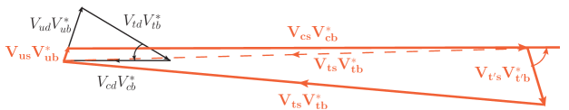
Figure 4: The $b\to d$ and $b\to s$ triangles of SM3, and the $b\to s$ quadrangle of SM4, with $V_{t^{\prime}s}V_{t^{\prime}b}^{*}$ taken from Eq. (9).

IV Implications and Discussion

We would like to give some interpretation of the impact of this possible future extraction of $\phi_{sb}$ and $r_{sb}$. We illustrate with the relatively aggressive value of Eq. (9), which corresponds to $\sin 2\Phi_{B_{s}}=-0.3\pm 0.1$ and ${\cal B}(B_{s}\to\mu^{+}\mu^{-})=(5.0\pm 1.5)\times 10^{-9}$ both enhanced over SM3 values, and $m_{t^{\prime}}=550$ GeV. We note that Eq. (9) is consistent with the finding of Ref. Hou:2010mm , but if it emerged in 2012, the information would be purely from these two measurements from the LHC, rather than from “global” considerations Buras:2010pi ; Soni:2010xh ; Eberhardt:2010bm ; Hou:2010mm .

A measurement like Eq. (9) would complete the unitarity quadrangle of Eq. (1), assuming, of course that one only established SM4 but no further new physics. Let us start by drawing the familiar SM3 $b\to d$ triangle, $V_{ud}V_{ub}^{*}+V_{cd}V_{cb}^{*}+V_{td}V_{tb}^{*}=0$, in Fig. 4. By standard convention PDG , $-V_{cd}V_{cb}^{*}$ is real and positive, $V_{ud}V_{ub}^{*}$ points above the real axis, while $V_{td}V_{tb}^{*}$ points from $V_{ud}V_{ub}^{*}$ to $-V_{cd}V_{cb}^{*}$, giving the familiar apex angle $\beta/\phi_{1}$, as indicated. Switching from $b\to d$ to $b\to s$, $V_{us}V_{ub}^{*}$ shrinks by $|V_{us}/V_{ud}|\simeq 0.23$ in length, but it is in the same direction as $V_{ud}V_{ub}^{*}$. The real and positive $V_{cs}V_{cb}^{*}$ extends parallel to the real axis from $V_{us}V_{ub}^{*}$ (most presentations by the experiments misrepresent this), but it is $|V_{cs}/V_{cd}|\simeq 1/0.22$ times longer than $-V_{cd}V_{cb}^{*}$. If $V_{t^{\prime}s}V_{t^{\prime}b}^{*}=0$, then $V_{ts}V_{tb}^{*}$ brings one straight back to the origin (dashed line in Fig. 4), i.e. $V_{us}V_{ub}^{*}+V_{cs}V_{cb}^{*}\equiv-V_{ts}V_{tb}^{*}|^{\rm SM3}$: one has a rather squashed SM3 $b\to s$ triangle with tiny $\Phi_{B_{s}}|^{\rm SM}$, but the same area as the $b\to d$ triangle.

But with $V_{t^{\prime}s}V_{t^{\prime}b}^{*}$ finite as in Eq. (9), $V_{ts}V_{tb}^{*}$ would now differ from $V_{ts}V_{tb}^{*}|^{\rm SM3}$, and carry a larger CPV phase itself. The quadrangle of Eq. (1), as shown in Fig. 4, would be larger in area than the $b\to d$ or $b\to s$ triangles in SM3 by a factor $|V_{t^{\prime}s}V_{t^{\prime}b}^{*}|/|V_{us}V_{ub}^{*}|\sim 0.0065/0.00088\simeq 7$, as the strength of phase angle is similar.

Equation (9) corresponds to $\sin 2\Phi_{B_{s}}$ that is $\sim 2\sigma$ away from the current LHCb central value of Eq. (2), and may not be realized. Equation (2) prefers a small $\sin 2\Phi_{B_{s}}$ value. With the large $r_{sb}$ possibilities ruled out by $A_{\rm FB}$ as discussed, one is left with $r_{sb}\equiv|V_{t^{\prime}s}V_{t^{\prime}b}^{*}|\lesssim 0.004$, with $\phi_{sb}$ practically unconstrained at present. One can picture this in Fig. 4 by reducing the length of $|V_{t^{\prime}s}V_{t^{\prime}b}^{*}|$ by 60%, and with the full 360^∘ $\phi_{sb}$ area allowed. This would probably need more data than 2011-2012 to measure.

The LHCb result Raven for $B_{s}\to J/\psi\phi$ alone gave a positive central value of $\sin\phi_{s}=0.13$. If this situation is borne out, we note from Fig. 2(b) that the branch for small and positive $\phi_{sb}$ is ruled out by $A_{\rm FB}$. But, depending on what ${\cal B}(B_{s}\to\mu^{+}\mu^{-})$ value turns up, there is a strip of allowed domain for $\phi_{sb}\in(200^{\circ},\ 330^{\circ})$. Following roughly the $\sin 2\Phi_{B_{s}}=+0.06$ dashed line on the righthand side of Fig. 2(b), the region above Case B and C (see also Fig. 3(a)) would be inferred. Larger $r_{sb}$ values for $\phi_{sb}\simeq 320^{\circ}$–$330^{\circ}$ would again be ruled out by $A_{\rm FB}$, but otherwise $A_{\rm FB}$ for this region would be quite consistent with SM3. The $b\to s$ quadrangle could again be easily drawn, with $r_{sb}$ typically in 0.004 to 0.005 range.

We note here a curiosity. In Fig. 1(a), the dashed curves correspond to SM3 contours, in the presence of $t^{\prime}$. Comparing with Fig. 3, the upper left and right curves are ruled out by $A_{\rm FB}$. The two vertical dashed lines in Fig. 1(a) corresponds to $V_{t^{\prime}s}V_{t^{\prime}b}^{*}$ being “parallel” to $V_{ts}V_{tb}^{*}|^{\rm SM3}$. The quadrangle of Eq. (1) would then become degenerate with SM3 hence have the same area.

We now offer a few points for further discussion.

The importance of measuring the SM4 $b\to s$ quadrangle cannot be overemphasized. It not only reflects possible new physics discoveries in $\sin 2\Phi_{B_{s}}$ and $B_{s}\to\mu^{+}\mu^{-}$, but interpreting via Fig. 4 may relate Hou:2008xd the measurement to BAU. Following the steps of Ref. Huet:1994jb , assuming a first-order phase transition, the generated BAU seems to be in the right ballpark HKK11 . Of course, Ref. Huet:1994jb may not apply to heavy $m_{t^{\prime}}$, but the nontrivial step of extending the computation into strong Yukawa coupling may address the other questionable assumption of order of phase transition. The problem is too important to be brushed aside just because of current inadequacies. We have also checked HHX11 that the neutron electric dipole moment could get enhanced to $10^{-31}$ $e\,$cm order, but it seems safely below the $10^{-28}$ $e\,$cm reach of the new generation of experiments, even with hadronic enhancement. As for the same-sign dilepton asymmetry uncovered by D0, although SM4 can give large and negative $\sin 2\Phi_{B_{s}}$, it cannot affect $b\to c\bar{c}s$ decay, and here we await the cross-check by LHCb.

A recent “global fit” (in contrast to others Buras:2010pi ; Soni:2010xh ; Eberhardt:2010bm ; Hou:2010mm ) of SM4 parameters found a rather small $|V_{t^{\prime}s}^{*}V_{t^{\prime}b}|<10^{-3}$ Alok:2010zj . This could be due to two inputs: allowing the central value of 1.04 (which violates unitarity) for $|V_{cs}|$, with an error of 0.06, may have inadvertently overconstrained $|V_{t^{\prime}s}|$; holding to the 2% lattice error for $\xi\equiv f_{B_{s}}^{2}\hat{B}_{B_{s}}/f_{B_{d}}^{2}\hat{B}_{B_{d}}$ (with $\Delta m_{B_{s}}/\Delta m_{B_{d}}$ precisely measured) in their fit, but not allowing the larger values of Eqs. (7) and (8) as possible future input, may be too strong a bias. We should add that the authors of Ref. Alok:2010zj did not include the hints for sizable $\sin 2\Phi_{B_{s}}$ into their fits. In any event, looking at Table III of Ref. Alok:2010zj , it seems unreasonable that $|V_{t^{\prime}s}^{*}V_{t^{\prime}b}|<10^{-3}$, while $|V_{t^{\prime}d}^{*}V_{t^{\prime}b}|>10^{-3}$ is allowed, especially when we are just entering the era for major progress in $b\to s$ measurements. A small $|V_{t^{\prime}s}^{*}V_{t^{\prime}b}|$ is certainly possible, but the three measurements stressed in this work would soon dominate the determination.

Why do we retain the SM3 $b\to d$ triangle, even when we extend to the SM4 $b\to s$ quadrangle? This point was addressed in the semiglobal analysis of Ref. Hou:2005yb . When considering kaon constraints on $V_{t^{\prime}d}^{*}V_{t^{\prime}s}$, a CKM unitarity approach showed that $V_{t^{\prime}d}V_{t^{\prime}b}^{*}$ and $V_{td}V_{tb}^{*}$ are relatively colinear with $V_{td}V_{tb}^{*}|^{\rm SM3}$, and cannot be easily distinguished by the $\sin 2\phi_{1}/\beta$ measurement. This, in fact, predated the subsequent realization of some tension in $B_{d}$ mixing and/or $\epsilon_{K}$ Lunghi:2008aa , and would require Super B factory and kaon studies to disentangle.

We have used $m_{t^{\prime}}=550$ GeV, which is at the unitarity bound, for our discussion. This value can be uncovered by direct search by 2012. If, however, the $t^{\prime}$ and $b^{\prime}$ quarks are above the UB, i.e $m_{t^{\prime}}\gtrsim 550$ GeV, then the 14 TeV run would be necessary. However, with the Yukawa coupling turned nonperturbative, the phenomenology may change Enkhbat:2011vp . On the other hand, we would definitely learn in the next two years whether $\sin 2\Phi_{B_{s}}$ and $B_{s}\to\mu^{+}\mu^{-}$ are beyond SM3 expectations.

Finally, we should mentioned that if a Higgs boson with SM3-like cross section and properties emerge at the LHC, indications of which could appear by end of 2011, SM4 alone would be in great difficulty Djouadi . One would have to extend beyond simple SM4, even if SM-like $t^{\prime}$ and $b^{\prime}$ quarks are found. On the other hand, the standard Higgs of SM3 itself, with mass below 600 GeV or so, might get ruled out by 2012. If such is the case, then we might enter the heavy–Higgs, heavy–quark world of SM4 Enkhbat:2011vp . We are in exciting times indeed.

V Conclusion

In conclusion, although once again SM3 seems to hold sway, whether time-dependent CPV in $B_{s}\to J/\psi\phi$ is considerably stronger than SM3 expectations will be conclusively settled with the full 2011–2012 data at LHCb, while one could discover that $B_{s}\to\mu^{+}\mu^{-}$ is mildly enhanced. If such is the case, we have shown that the fourth generation $b\to s$ unitarity quadrangle would become measured, which could have a bearing on the matter-antimatter asymmetry of the Universe. The main thrusts in this quest at the LHC are $\sin 2\Phi_{B_{s}}$, ${\cal B}(B_{s}\to\mu^{+}\mu^{-})$ and $A_{\rm FB}(B^{0}\to K^{*0}\mu^{+}\mu^{-})$.

Acknowledgement. WSH thanks the National Science Council for an Academic Summit grant, NSC 100-2745-M-002-002-ASP, while MK and FX are supported under the NTU grant 10R40044 and the Laurel program.

Note Added. Immediately after submission of our work, we learned that CDF measured CDFmumu11 ${\cal B}(B_{s}\to\mu^{+}\mu^{-})=(18^{+11}_{\;-9})\times 10^{-9}$, which was countered by lower values from LHCb LHCb-mumu11 and CMS CMSmumu11 within a week. The subsequent rapid unfolding of the LHCb results of $A_{\rm FB}(B^{0}\to K^{*0}\mu^{+}\mu^{-})$ at EPS-HEP 2011, and $\sin\phi_{s}$ at LP 2011 was both exhilarating and somewhat disappointing, and resulted in major revision of this paper.

References

- (1) K. Nakamura et al. [Particle Data Group], J. Phys. G 37, 075021 (2010).
- (2) M. Kobayashi and T. Maskawa, Prog. Theor. Phys. 49, 652 (1973).
- (3) N. Cabibbo, Phys. Rev. Lett. 10, 531 (1963).
- (4) S.L. Glashow, J. Iliopoulos and L. Maiani, Phys. Rev. D 2, 1285 (1970).
- (5) S.-W. Lin et al. [Belle Collaboration], Nature 452, 332 (2008).
- (6) W.-S. Hou, M. Nagashima and A. Soddu, Phys. Rev. Lett. 95, 141601 (2005).
- (7) W.-S. Hou, M. Nagashima and A. Soddu, Phys. Rev. D 72, 115007 (2005).
- (8) W.-S. Hou, M. Nagashima and A. Soddu, Phys. Rev. D 76, 016004 (2007).
- (9) The LHCb Collaboration, LHCb-CONF-2011-006.
- (10) Plenary talk by G. Raven at Lepton Photon Symposium, August 2011, Mumbai, India.
- (11) G.D. Kribs et al., Phys. Rev. D 76, 075016 (2007); H.-J. He, N. Polonsky and S.-f. Su, Phys. Rev. D 64, 053004 (2001); V.A. Novikov, L.B. Okun, A.N. Rozanov and M.I. Vysotsky, JETP Lett. 76, 127 (2002) [Pisma Zh. Eksp. Teor. Fiz. 76, 158 (2002)].
- (12) For a recent brief review on the fourth generation, see B. Holdom et al. PMC Phys. A 3, 4 (2009).
- (13) S. Chatrchyan et al. [CMS Collaboration], Phys. Lett. B 701, 204 (2011).
- (14) Plenary talk by A. De Roeck at Lepton Photon Symposium, August 2011, Mumbai, India.
- (15) M.S. Chanowitz, M.A. Furman and I. Hinchliffe, Phys. Lett. B 78, 285 (1978).
- (16) R. Aaij et al. [LHCb Collaboration], Phys. Lett. B 699, 330 (2011).
- (17) A.J. Buras et al., JHEP 1009, 106 (2010).
- (18) The combined summer 2011 limit of LHCb and CMS on can be found in the documents LHCb-CONF-2011-043 and CMS PAS BPH-11-019.
- (19) A. Soni et al., Phys. Rev. D 82, 033009 (2010).
- (20) O. Eberhardt, A. Lenz and J. Rohrwild, Phys. Rev. D 82, 095006 (2010).
- (21) E. Golowich et al., Phys. Rev. D 83, 114017 (2011).
- (22) W.-S. Hou, Chin. J. Phys. 47, 134 (2009).
- (23) A.J. Buras, Phys. Lett. B 566, 115 (2003).
- (24) W.-S. Hou and C.-Y. Ma, Phys. Rev. D 82, 036002 (2010).
- (25) A.G. Akeroyd, F. Mahmoudi and D.M. Santos, arXiv:1108.3018.
- (26) Talk by M. Patel at EPS-HEP Conference, July 2011, Grenoble, France.
- (27) P. Ball and R. Zwicky, Phys. Rev. D 71 (2005) 014029; M. Beneke, T. Feldmann and D. Seidel, Nucl. Phys. B 612 (2001) 25.
- (28) P. Huet and E. Sather, Phys. Rev. D 51, 379 (1995).
- (29) W.-S. Hou, Y. Kikukawa and M. Kohda, unpublished.
- (30) J. Hisano, W.-S. Hou and F. Xu, arXiv:1107.3642 [Phys. Rev. D (to be published)].
- (31) A.K. Alok, A. Dighe and D. London, Phys. Rev. D 83, 073008 (2011).
- (32) E. Lunghi and A. Soni, Phys. Lett. B 666, 162 (2008); A.J. Buras and D. Guadagnoli, Phys. Rev. D 78, 033005 (2008).
- (33) See, for example, the discussion by T. Enkhbat, W.-S. Hou and H. Yokoya, arXiv:1109.3382.
- (34) Plenary talk by A. Djouadi at Lepton Photon Symposium, August 2011, Mumbai, India.
- (35) T. Aaltonen et al. [CDF Collaboration], Phys. Rev. Lett. 107, 191801 (2011).
- (36) Talk by J. Serrano at EPS-HEP Conference, July 2011, Grenoble, France.
- (37) S. Chatrchyan et al. [CMS Collaboration], Phys. Rev. Lett. 107, 191802 (2011).