BSVM  

A Banded Support Vector Machine

Author:

Gautam V. Pendse
gpendse@mclean.harvard.edu

P.A.I.N Group, Brain Imaging Center
McLean Hospital, Harvard Medical School

Abstract

We describe a novel binary classification technique called Banded SVM (B-SVM). In the standard C-SVM formulation of Cortes and Vapnik (1995), the decision rule is encouraged to lie in the interval $[1,\infty]$. The new B-SVM objective function contains a penalty term that encourages the decision rule to lie in a user specified range $[\rho_{1},\rho_{2}]$. In addition to the standard set of support vectors (SVs) near the class boundaries, B-SVM results in a second set of SVs in the interior of each class.

Notation

• Scalars and functions will be denoted in a non-bold font (e.g., $\beta_{0},C,g$). Vectors and vector functions will be denoted in a bold font using lower case letters (e.g., $\boldsymbol{x},\boldsymbol{\beta},\boldsymbol{h}$). Matrices will be denoted in bold font using upper case letters (e.g., $\boldsymbol{B},\boldsymbol{H}$). The transpose of a matrix $\boldsymbol{A}$ will be denoted by $\boldsymbol{A^{T}}$ and its inverse will be denoted by $\boldsymbol{A^{-1}}$. $\boldsymbol{I_{p}}$ will denote the $p\times p$ identity matrix and $\mathbf{0}$ will denote a vector or matrix of all zeros whose size should be clear from context.

• $|x|$ will denote the absolute value of $x$ and $\mathcal{I}(x>a)$ is an indicator function that returns $1$ if $x>a$ and $0$ otherwise.

• The $j$th component of vector $\boldsymbol{t}$ will be denoted by $t_{j}$. The element $(i,j)$ of matrix $\boldsymbol{G}$ will be denoted by $G(i,j)$ or $G_{ij}$. The 2-norm of a $p\times 1$ vector $\boldsymbol{x}$ will be denoted by $||\boldsymbol{x}||_{2}=+\sqrt{\sum_{i=1}^{p}x_{i}^{2}}$. Probability distribution of a random vector $\boldsymbol{x}$ will be denoted by $\mathbf{P}_{\boldsymbol{x}}(\boldsymbol{x})$. $\mathbf{E}\left[f(\boldsymbol{s},\boldsymbol{\eta})\right]$ denotes the expectation of $f(\boldsymbol{s},\boldsymbol{\eta})$ with respect to both random variables $\boldsymbol{s}$ and $\boldsymbol{\eta}$.

1 Introduction

We consider the standard binary classification problem. Suppose $y_{i}$ is the class membership label ($+1$ for class $+1$ and $-1$ for class $-1$) associated with a feature vector $\boldsymbol{x_{i}}$. Given $n$ such $(\boldsymbol{x_{i}},y_{i})$ pairs, we would like to learn a linear decision rule $g(\boldsymbol{x})$ that can be used to accurately predict the class label $y$ associated with feature vector $\boldsymbol{x}$.

In C-SVM (Vapnik and Lerner, 1963; Boser et al., 1992; Cortes and Vapnik, 1995), one can think of the linear decision rule $g$ as a means of measuring membership in a particular class. Given a feature vector $\boldsymbol{x}$, C-SVM encourages the function $g(\boldsymbol{x})$ to be positive if $\boldsymbol{x}\in$ class $+1$ and negative if $\boldsymbol{x}\in$ class $-1$.

We motivate the development of B-SVM in the following way. Suppose that vector $\boldsymbol{x}$ comes from an arbitrary probability distribution $\mathbf{P}_{\boldsymbol{x}}(\boldsymbol{x})$ with mean $\mathbf{E}[\boldsymbol{x}]=\boldsymbol{\mu}$ and finite co-variance $\mbox{Cov}[\boldsymbol{x}]=\boldsymbol{\Sigma}$. Consider the linear decision rule $g(\boldsymbol{x})=\boldsymbol{\beta}^{T}\boldsymbol{x}+\beta_{0}$. It is easy to see that $g(\boldsymbol{x})$ has mean $\mathbf{E}[g(\boldsymbol{x})]=\boldsymbol{\beta}^{T}\boldsymbol{\mu}+\beta_{0}$ and covariance $\mbox{Cov}[g(\boldsymbol{x})]=\boldsymbol{\beta}^{T}\boldsymbol{\Sigma}\boldsymbol{\beta}$. By Chebyshev’s inequality, there exists a high probability band around $\mathbf{E}[g(\boldsymbol{x})]$ where $g(\boldsymbol{x})$ is expected to lie when $\boldsymbol{x}$ comes from $\mathbf{P}_{\boldsymbol{x}}(\boldsymbol{x})$.

Hence, for every probability distribution of vectors $\boldsymbol{x}$ from class $+1$ and class $-1$ with finite co-variance, $g(\boldsymbol{x})$ is expected to lie in a certain high probability band. In B-SVM, we choose $g(\boldsymbol{x})$ to encourage:

• $y\,g(\boldsymbol{x})>0\,\,\,$ 🖘  same condition as C-SVM

• $y\,g(\boldsymbol{x})\in\mbox{certain high probability {{band}}}\,\,\,$ 🖘  new B-SVM condition

Both of the above conditions can be satisfied if we encourage:

$$\boxed{y\,g(\boldsymbol{x})\in[\rho_{1},\rho_{2}]\mbox{ with }\rho_{2}>\rho_{1}>0}$$ (1.1)

Since non-linear decision rules in C-SVM are simply linear decision rules operating in a high dimensional space via the kernel trick (Boser et al., 1992), the B-SVM band formation argument holds for non-linear decision rules as well.

2 Problem setup

As per standard SVM terminology, assume that we are given $n$ data-label pairs $(\boldsymbol{x_{i}},y_{i})$ where $\boldsymbol{x_{i}}$ are $m\times 1$ vectors and the data labels $y_{i}\in\{-1,1\}$. First, we consider only the linear case and afterwards transform to the general case via the kernel trick. Let $m\times 1$ vector $\boldsymbol{\beta}$ and scalar $\beta_{0}$ be parameters of a linear decision rule $g(\boldsymbol{x})=\boldsymbol{\beta}^{T}\boldsymbol{x}+\beta_{0}=0$ separating class $+1$ and $-1$ such that $g(\boldsymbol{x})>0$ if $\boldsymbol{x}$ belongs to class $+1$ and vice versa.

2.1 C-SVM objective function

The C-SVM objective function (Cortes and Vapnik, 1995) to be minimized can be written as:

$$f_{CSVM}(\boldsymbol{\beta},\beta_{0})=\frac{1}{2}||\boldsymbol{\beta}||^{2}_{2}+C\sum_{i=1}^{n}[1-y_{i}(\boldsymbol{\beta}^{T}\boldsymbol{x_{i}}+\beta_{0})]_{+}$$ (2.1)

where $[t]_{+}$ is the positive part of $t$:

$$[t]_{+}=\begin{cases}0&\text{if $t\leq 0$},\\ t&\text{if $t>0$}.\end{cases}$$ (2.2)

and $C$ governs the regularity of the solution. The C-SVM objective function penalizes signed decisions $y_{i}(\boldsymbol{\beta}^{T}\boldsymbol{x_{i}}+\beta_{0})$ whenever their value is below 1. This is the only penalty in C-SVM.

2.2 B-SVM objective function

We present below the novel B-SVM objective function that we wish to minimize:

$$f_{BSVM}(\boldsymbol{\beta},\beta_{0})=\frac{1}{2}||\boldsymbol{\beta}||^{2}_{2}\,+\,\underbracket{C_{1}\sum_{i=1}^{n}[\rho_{1}-y_{i}(\boldsymbol{\beta}^{T}\boldsymbol{x_{i}}+\beta_{0})]_{+}}_{\mbox{{\color[rgb]{1,0,0}C-SVM like penalty}}}\,+\,\underbracket{C_{2}\sum_{i=1}^{n}[y_{i}(\boldsymbol{\beta}^{T}\boldsymbol{x_{i}}+\beta_{0})-\rho_{2}]_{+}}_{\mbox{{\color[rgb]{1,0,0}novel B-SVM penalty}}}$$ (2.3)

where $\rho_{2}>\rho_{1}>0$ are margin parameters specified by the user and $C_{1}$ and $C_{2}$ are regularization constants. This objective function has two penalty terms:

• The first penalty term is similar to C-SVM. It penalizes signed decisions $y_{i}(\boldsymbol{\beta}^{T}\boldsymbol{x_{i}}+\beta_{0})$ whenever their values are below $\rho_{1}$ (as opposed to 1 in C-SVM).

• The second penalty term is novel. It penalizes signed decisions $y_{i}(\boldsymbol{\beta}^{T}\boldsymbol{x_{i}}+\beta_{0})$ when their values are above $\rho_{2}$.

The net effect of these penalty terms is to encourage $y_{i}(\boldsymbol{\beta}^{T}\boldsymbol{x_{i}}+\beta_{0})$ to lie in the interval $[\rho_{1},\rho_{2}]$. Please see Figure 1 for a sketch of the two penalty terms in B-SVM.

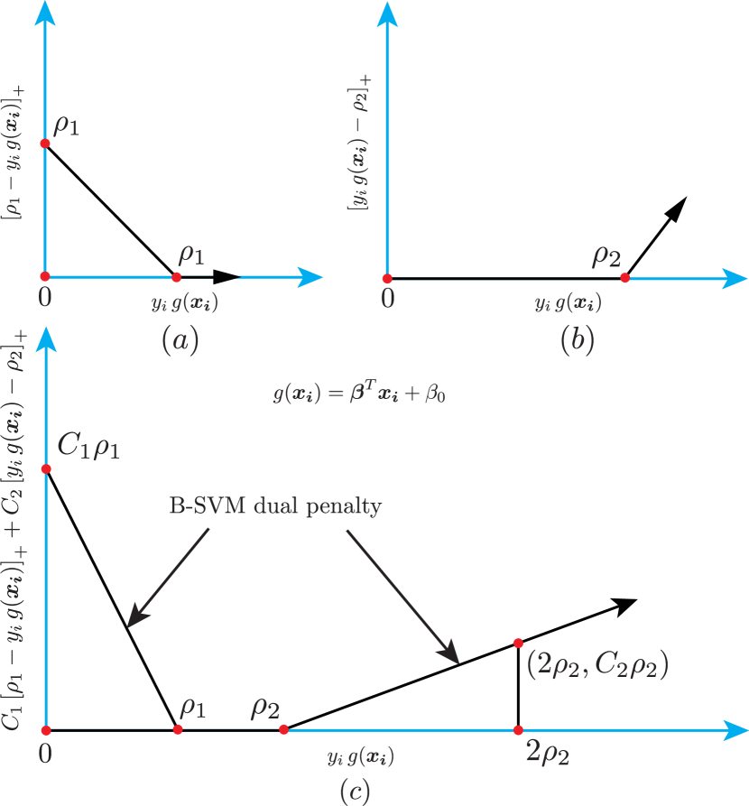
Figure 1: (a) Standard C-SVM like penalty function penalizes $y_{i}(\boldsymbol{\beta}^{T}\boldsymbol{x_{i}}+\beta_{0})<\rho_{1}$. In B-SVM, $\rho_{1}$ replaces the constant $1$ from C-SVM. (b) Novel B-SVM penalty function. This function penalizes $y_{i}(\boldsymbol{\beta}^{T}\boldsymbol{x_{i}}+\beta_{0})>\rho_{2}$. (c) Total penalty function for B-SVM. If $y_{i}(\boldsymbol{\beta}^{T}\boldsymbol{x_{i}}+\beta_{0})\in[\rho_{1},\rho_{2}]$ then the total penalty is $0$. Choosing $C_{2}<C_{1}$ will impose a milder penalty for values of $y_{i}(\boldsymbol{\beta}^{T}\boldsymbol{x_{i}}+\beta_{0})>\rho_{2}$.

3 Solving the B-SVM problem

We derive the B-SVM dual problem in order to maximize a lower bound on the B-SVM primal objective function in equation 2.3. This dual problem will be simpler to solve compared to the primal form 2.3. We proceed as follows:

• As shown in 3.2, the primal problem in 2.3 can be modified into a strictly convex objective function with linear inequality constraints using slack variables.

• Consequently, strong duality holds and the maximum value of the B-SVM dual objective function is equal to the minimum value of the B-SVM primal objective function in 2.3.

For more details on convex duality, please see Nocedal and Wright (2006).

3.1 The B-SVM dual problem

We introduce slack variables:

$$\xi_{i} =[\rho_{1}-y_{i}(\boldsymbol{\beta}^{T}\boldsymbol{x_{i}}+\beta_{0})]_{+}$$ (3.1)

$$\eta_{i} =[y_{i}(\boldsymbol{\beta}^{T}\boldsymbol{x_{i}}+\beta_{0})-\rho_{2}]_{+}$$

into the primal objective function in 2.3. The modified optimization problem can be written as:

$$\min_{\boldsymbol{\beta},\beta_{0},\boldsymbol{\xi},\boldsymbol{\eta}}f_{BSVM}(\boldsymbol{\beta},\beta_{0},\boldsymbol{\xi},\boldsymbol{\eta}) =\frac{1}{2}||\boldsymbol{\beta}||^{2}_{2}+C_{1}\sum_{i=1}^{n}\xi_{i}+C_{2}\sum_{i=1}^{n}\eta_{i}$$ (3.2)

$$\xi_{i} \geq 0 \mu_{i}$$ Lagrange multiplier

$$\eta_{i} \geq 0 \psi_{i}$$ Lagrange multiplier

$$\xi_{i} \geq\rho_{1}-y_{i}(\boldsymbol{\beta}^{T}\boldsymbol{x_{i}}+\beta_{0}) \alpha_{i}$$ Lagrange multiplier

$$\eta_{i} \geq-\rho_{2}+y_{i}(\boldsymbol{\beta}^{T}\boldsymbol{x_{i}}+\beta_{0}) \theta_{i}$$ Lagrange multiplier

After introducing Lagrange multipliers for each inequality constraint as shown in 3.2, the Lagrangian function for problem 3.2 can be written as:

$$L(\boldsymbol{\beta},\beta_{0},\boldsymbol{\xi},\boldsymbol{\eta},\boldsymbol{\alpha},\boldsymbol{\theta},\boldsymbol{\mu},\boldsymbol{\psi})=\frac{1}{2}||\boldsymbol{\beta}||^{2}_{2}\,+\, C_{1}\sum_{i=1}^{n}\xi_{i}+C_{2}\sum_{i=1}^{n}\eta_{i}-\sum_{i=1}^{n}\alpha_{i}\{\xi_{i}-\rho_{1}+y_{i}(\boldsymbol{\beta}^{T}\boldsymbol{x_{i}}+\beta_{0})\}$$ (3.3)

$$-\sum_{i=1}^{n}\theta_{i}\{\eta_{i}+\rho_{2}-y_{i}(\boldsymbol{\beta}^{T}\boldsymbol{x_{i}}+\beta_{0})\}-\sum_{i=1}^{n}\mu_{i}\xi_{i}-\sum_{i=1}^{n}\psi_{i}\eta_{i}$$

where

$$\alpha_{i},\theta_{i},\mu_{i},\psi_{i}\geq 0$$ (3.4)

Next, we solve for primal variables $\boldsymbol{\beta},\beta_{0},\boldsymbol{\xi},\boldsymbol{\eta}$ in terms of the dual variables $\boldsymbol{\alpha},\boldsymbol{\theta},\boldsymbol{\mu},\boldsymbol{\psi}$ by minimizing $L(\boldsymbol{\beta},\beta_{0},\boldsymbol{\xi},\boldsymbol{\eta},\boldsymbol{\alpha},\boldsymbol{\theta},\boldsymbol{\mu},\boldsymbol{\psi})$ with respect to the primal variables. Since the Lagrangian in 3.3 is a convex function of the primal variables, its unique global minimum can be obtained using the first order Karush Kuhn Tucker (KKT) conditions given in 3.5 - 3.8:

$$\frac{\partial L}{\partial\boldsymbol{\beta}}=\boldsymbol{\beta}-\sum_{i=1}^{n}\alpha_{i}y_{i}\boldsymbol{x_{i}}+\sum_{i=1}^{n}\theta_{i}y_{i}\boldsymbol{x_{i}}=0$$ (3.5)

$$\frac{\partial L}{\partial\beta_{0}}=-\sum_{i=1}^{n}\alpha_{i}y_{i}+\sum_{i=1}^{n}\theta_{i}y_{i}=0$$ (3.6)

$$\frac{\partial L}{\partial\xi_{l}}=C_{1}-\alpha_{l}-\mu_{l}=0$$ (3.7)

$$\frac{\partial L}{\partial\eta_{l}}=C_{2}-\theta_{l}-\psi_{l}=0$$ (3.8)

From 3.5, the vector $\boldsymbol{\beta}$ is given by:

$$\boldsymbol{\beta}=\sum_{i=1}^{n}(\alpha_{i}-\theta_{i})\,y_{i}\,\boldsymbol{x_{i}}$$ (3.9)

From 3.6, vectors $\boldsymbol{\alpha}$ and $\boldsymbol{\theta}$ satisfy the equality constraint:

$$\sum_{i=1}^{n}(\alpha_{i}-\theta_{i})\,y_{i}=0$$ (3.10)

Combining 3.7, 3.8 and 3.4, the elements of $\boldsymbol{\alpha}$ must satisfy:

$$0\leq\alpha_{i}\leq C_{1}$$ (3.11)

and elements of $\boldsymbol{\theta}$ satisfy:

$$0\leq\theta_{i}\leq C_{2}$$ (3.12)

Let $\boldsymbol{B}$ be a $n\times n$ matrix with entries:

$$B_{ij}=y_{i}y_{j}\,\boldsymbol{x_{i}}^{T}\boldsymbol{x_{j}}$$ (3.13)

and $\boldsymbol{e}_{n}$ be a $n\times 1$ vector of $n$ ones (in MATLAB notation: $\boldsymbol{e}_{n}$ = ones(n,1)). Substituting $\boldsymbol{\beta}$ from 3.9 in 3.3 and noting the constraints 3.7, 3.8 and 3.10, we get the B-SVM dual problem:

$$\max_{\boldsymbol{\alpha},\boldsymbol{\theta}}L_{D}(\boldsymbol{\alpha},\boldsymbol{\theta}) =\rho_{1}\,\boldsymbol{e}^{T}_{n}\boldsymbol{\alpha}-\rho_{2}\,\boldsymbol{e}^{T}_{n}\boldsymbol{\theta}-\frac{1}{2}(\boldsymbol{\alpha}-\boldsymbol{\theta})^{T}\boldsymbol{B}(\boldsymbol{\alpha}-\boldsymbol{\theta})$$ (3.14)

$$\boldsymbol{0}\leq\boldsymbol{\alpha}\leq C_{1}\,\boldsymbol{e}_{n}$$

$$\boldsymbol{0}\leq\boldsymbol{\theta}\leq C_{2}\,\boldsymbol{e}_{n}$$

$$(\boldsymbol{\alpha}-\boldsymbol{\theta})^{T}\boldsymbol{y}=0$$

If $C_{2}=0$ and $\rho_{1}=1$ then 3.12 implies $\boldsymbol{\theta}=\boldsymbol{0}$ and hence we recover the standard C-SVM dual problem.

3.2 Kernelifying B-SVM

Let $\boldsymbol{h}$ be a non-linear vector function that takes inputs $\boldsymbol{x_{i}}$ into a high dimensional space. Then we recover kernel B-SVM by doing linear B-SVM on the data-label pairs $(\boldsymbol{h}(\boldsymbol{x_{i}}),y_{i})$ instead of the original pairs $(\boldsymbol{x_{i}},y_{i})$. In practice, we do not need $\boldsymbol{h}(\boldsymbol{x})$ explicitly but only the dot products through a kernel matrix $\boldsymbol{K}$ with elements:

$$K_{ij}=K(\boldsymbol{x_{i}},\boldsymbol{x_{j}})=\boldsymbol{h}(\boldsymbol{x_{i}})^{T}\boldsymbol{h}(\boldsymbol{x_{j}})$$ (3.15)

This is the so-called kernel trick. From 3.13, elements of matrix $\boldsymbol{B}$ for transformed feature vectors $\boldsymbol{h}(\boldsymbol{x})$ are given by:

$$B_{ij}=y_{i}y_{j}\,\boldsymbol{h}(\boldsymbol{x_{i}})^{T}\boldsymbol{h}(\boldsymbol{x_{j}})=y_{i}y_{j}\,K_{ij}=y_{i}y_{j}\,K(\boldsymbol{x_{i}},\boldsymbol{x_{j}})$$ (3.16)

For a new point $\boldsymbol{x}$, the decision rule is then given by:

$$g(\boldsymbol{x})=\boldsymbol{\beta}^{T}\boldsymbol{h}(\boldsymbol{x})+\beta_{0}$$ (3.17)

and $\boldsymbol{x}$ is classified into class $+1$ if $g(\boldsymbol{x})>0$ and into class $-1$ if $g(\boldsymbol{x})<0$. From 3.9, for the transformed feature vectors $\boldsymbol{h}(\boldsymbol{x_{i}})$, we have:

$$\boldsymbol{\beta}=\sum_{i=1}^{n}(\alpha_{i}-\theta_{i})\,y_{i}\,\boldsymbol{h}(\boldsymbol{\boldsymbol{x_{i}}})$$ (3.18)

Using the kernel trick, calculation of $g(\boldsymbol{x})$ does not need $\boldsymbol{h}(\boldsymbol{x})$ explicitly as we can write:

$$\boxed{g(\boldsymbol{x})=\boldsymbol{\beta}^{T}\boldsymbol{h}(\boldsymbol{x})+\beta_{0}=\sum_{i=1}^{n}(\alpha_{i}-\theta_{i})\,y_{i}\,K(\boldsymbol{x_{i}},\boldsymbol{x})+\beta_{0}}$$ (3.19)

Proposition 3.1.

The B-SVM dual objective function $L_{D}(\boldsymbol{\alpha},\boldsymbol{\theta})$ in 3.14 is a concave function of $\boldsymbol{\alpha}$ and $\boldsymbol{\theta}$.

Proof.

Since $\boldsymbol{B}$ is symmetric, the Hessian of $L_{D}$ with respect to the vector $(\boldsymbol{\alpha},\boldsymbol{\theta})$ is given by:

$$\boldsymbol{H}=\begin{pmatrix}-\boldsymbol{B}&\boldsymbol{B}\\ \boldsymbol{B}&-\boldsymbol{B}\end{pmatrix}$$ (3.20)

If $\boldsymbol{c}$ and $\boldsymbol{d}$ are arbitrary $n\times 1$ vectors,

$$\begin{pmatrix}\boldsymbol{c}^{T}&\boldsymbol{d}^{T}\end{pmatrix}\boldsymbol{H}\begin{pmatrix}\boldsymbol{c}\\ \boldsymbol{d}\end{pmatrix}=\boldsymbol{c}^{T}(-\boldsymbol{B}\boldsymbol{c}+\boldsymbol{B}\boldsymbol{d})+\boldsymbol{d}^{T}(\boldsymbol{B}\boldsymbol{c}-\boldsymbol{B}\boldsymbol{d})=-(\boldsymbol{c}-\boldsymbol{d})^{T}\boldsymbol{B}\,(\boldsymbol{c}-\boldsymbol{d})$$ (3.21)

From 3.16,

$$(\boldsymbol{c}-\boldsymbol{d})^{T}\boldsymbol{B}\,(\boldsymbol{c}-\boldsymbol{d})=\sum_{i=1}^{n}\sum_{j=1}^{n}(\boldsymbol{c}-\boldsymbol{d})_{i}\{y_{i}y_{j}\boldsymbol{K}(\boldsymbol{x_{i}},\boldsymbol{x_{j}})\}(\boldsymbol{c}-\boldsymbol{d})_{j}=\sum_{i=1}^{n}\sum_{j=1}^{n}\{(\boldsymbol{c}-\boldsymbol{d})_{i}y_{i}\}\boldsymbol{K}(\boldsymbol{x_{i}},\boldsymbol{x_{j}})\{(\boldsymbol{c}-\boldsymbol{d})_{j}y_{j}\}$$ (3.22)

If $\odot$ is an element-wise multiplication operator then:

$$(\boldsymbol{c}-\boldsymbol{d})^{T}\boldsymbol{B}\,(\boldsymbol{c}-\boldsymbol{d})=\{(\boldsymbol{c}-\boldsymbol{d})\odot\boldsymbol{y}\}^{T}\boldsymbol{K}\{(\boldsymbol{c}-\boldsymbol{d})\odot\boldsymbol{y}\}\geq 0$$ (3.23)

where the last inequality holds since $\boldsymbol{K}$ is a kernel matrix which is positive definite by 3.15. Therefore, from 3.21 and 3.23:

$$\begin{pmatrix}\boldsymbol{c}^{T}&\boldsymbol{d}^{T}\end{pmatrix}\boldsymbol{H}\begin{pmatrix}\boldsymbol{c}\\ \boldsymbol{d}\end{pmatrix}\leq 0$$ (3.24)

for all vectors $\boldsymbol{c}$ and $\boldsymbol{d}$. Thus $L_{D}(\boldsymbol{\alpha},\boldsymbol{\theta})$ is a concave function of $(\boldsymbol{\alpha},\boldsymbol{\theta})$. ∎∎

It immediately follows that problem 3.14 attempts to maximize a concave function under linear constraints and thus has a unique solution (Nocedal and Wright, 2006).

3.3 Calculation of dual variables

Dual variables $\boldsymbol{\alpha}$, $\boldsymbol{\theta}$, $\boldsymbol{\mu}$, $\boldsymbol{\psi}$ can be calculated as follows:

• Calculation of $\boldsymbol{\alpha}$, $\boldsymbol{\theta}$ requires the solution of a concave maximization problem 3.14 where the elements of $\boldsymbol{B}$ are chosen using a suitable kernel $\boldsymbol{K}(\boldsymbol{x_{i}},\boldsymbol{x_{j}})$. This can be accomplished using an sequential minimal optimization (SMO) type active set technique (Platt, 1998) or a projected conjugate gradient (PCG) technique (Nocedal and Wright, 2006).

• Once $\boldsymbol{\alpha}$ and $\boldsymbol{\theta}$ are known, equations 3.7 and 3.8 give $\boldsymbol{\mu}=C_{1}\boldsymbol{e}_{n}-\boldsymbol{\alpha}$ and $\boldsymbol{\psi}=C_{2}\boldsymbol{e}_{n}-\boldsymbol{\theta}$.

3.4 Calculation of primal variables

Primal variables $\boldsymbol{\beta}$, $\boldsymbol{\beta_{0}}$, $\boldsymbol{\xi}$, $\boldsymbol{\eta}$ can be calculated as follows:

• $\boldsymbol{\beta}$ is given by equation 3.18.

• Calculation of $\boldsymbol{\beta_{0}}$, $\boldsymbol{\xi}$, $\boldsymbol{\eta}$ is accomplished by considering the inequality constraints and the KKT complementarity constraints for the problem 3.2:

  $$\xi_{i}\geq 0,\eta_{i}\geq 0$$ (3.25)

  $$\xi_{i}\geq\rho_{1}-y_{i}\left(\boldsymbol{\beta}^{T}\boldsymbol{h}(\boldsymbol{x_{i}})+\beta_{0}\right)$$

  $$\eta_{i}\geq-\rho_{2}+y_{i}\left(\boldsymbol{\beta}^{T}\boldsymbol{h}(\boldsymbol{x_{i}})+\beta_{0}\right)$$

  $$\alpha_{i}\{\xi_{i}-\rho_{1}+y_{i}\left(\boldsymbol{\beta}^{T}\boldsymbol{h}(\boldsymbol{x_{i}})+\beta_{0}\right)\}=0$$

  $$\theta_{i}\{\eta_{i}+\rho_{2}-y_{i}\left(\boldsymbol{\beta}^{T}\boldsymbol{h}(\boldsymbol{x_{i}})+\beta_{0}\right)\}=0$$

  $$\mu_{i}\xi_{i}=(C_{1}-\alpha_{i})\xi_{i}=0$$

  $$\psi_{i}\eta_{i}=(C_{2}-\theta_{i})\eta_{i}=0$$

  Given the positivity constraints 3.4 and the bound constraints 3.11 and 3.12, we consider the following cases:

  • If $\alpha_{i}<C_{1}$ then $\xi_{i}=0$ and similarly if $\theta_{i}<C_{2}$ then $\eta_{i}=0$.

  • If $0<\alpha_{i}<C_{1}$ then we have $\xi_{i}=0$ and $\{\xi_{i}-\rho_{1}+y_{i}(\beta^{T}x_{i}+\beta_{0})\}=0$ which can be used to solve for $\beta_{0}$.

  • If $0<\theta_{i}<C_{2}$ then we have $\eta_{i}=0$ and $\{\eta_{i}+\rho_{2}-y_{i}\left(\boldsymbol{\beta}^{T}\boldsymbol{h}(\boldsymbol{x_{i}})+\beta_{0}\right)\}=0$ which can be used to solve for $\beta_{0}$.

  • Similar to C-SVM, for stability purposes we can average the estimate of $\beta_{0}$ over all points where $0<\alpha_{i}<C_{1}$ and $0<\theta_{i}<C_{2}$.

  • We can calculate $\xi_{i}$ for those points for which $\alpha_{i}=C_{1}$ using $\xi_{i}=\rho_{1}-y_{i}\left(\boldsymbol{\beta}^{T}\boldsymbol{h}(\boldsymbol{x_{i}})+\beta_{0}\right)$.

  • Similarly, if $\theta_{i}=C_{2}$ then $\eta_{i}=y_{i}\left(\boldsymbol{\beta}^{T}\boldsymbol{h}(\boldsymbol{x_{i}})+\beta_{0}\right)-\rho_{2}$.

4 Toy data

In order to illustrate the differences between C-SVM and B-SVM we generated artificial data in 2 dimensions as follows:

• Class $1$ consisted of 5 bivariate Normal clusters centered at $(0,0)$, $(\frac{1}{\sqrt{2}},\frac{1}{\sqrt{2}})$, $(\frac{-1}{\sqrt{2}},\frac{1}{\sqrt{2}})$, $(\frac{-1}{\sqrt{2}},\frac{-1}{\sqrt{2}})$ and $(\frac{1}{\sqrt{2}},\frac{-1}{\sqrt{2}})$ and covariance $\sigma^{2}_{1}\boldsymbol{I}_{2}$ with $\sigma_{1}=0.2$.

• Class $-1$ consisted of 4 bivariate Normal clusters centered at $(1,0)$, $(0,1)$, $(-1,0)$ and $(0,-1)$ with covariacne $\sigma^{2}_{2}\boldsymbol{I}_{2}$ with $\sigma_{2}=0.2$.

A radial basis function (RBF) kernel was chosen for computations. For the RBF kernel, the elements of $\boldsymbol{K}$ are given by:

$$K(\boldsymbol{x_{i}},\boldsymbol{x_{j}})=K_{ij}=\mbox{exp}\left\{-\gamma\left(\boldsymbol{x_{i}}-\boldsymbol{x_{j}}\right)^{T}\left(\boldsymbol{x_{i}}-\boldsymbol{x_{j}}\right)\right\}$$ (4.1)

Our parameter settings were as follows:

• For both C-SVM and B-SVM we used the same kernel parameter $\gamma=1$.

• For C-SVM was used $C=10$.

• For B-SVM we chose $\rho_{1}=1$ and $C_{1}=10$ (same as $C$ for C-SVM). Thus the parameters of the common penalty term $C_{1}\sum_{i=1}^{n}[\rho_{1}-y_{i}(\boldsymbol{\beta}^{T}\boldsymbol{h}(\boldsymbol{x_{i}})+\beta_{0})]_{+}$ are chosen to be identical for C-SVM and B-SVM.

• The parameters of the second penalty term for B-SVM were chosen as $C_{2}=100$ and $\rho_{2}=1.5$. Thus B-SVM will encourage $g(\boldsymbol{x})$ to lie in the interval $[\rho_{1},\rho_{2}]=[1,1.5]$.

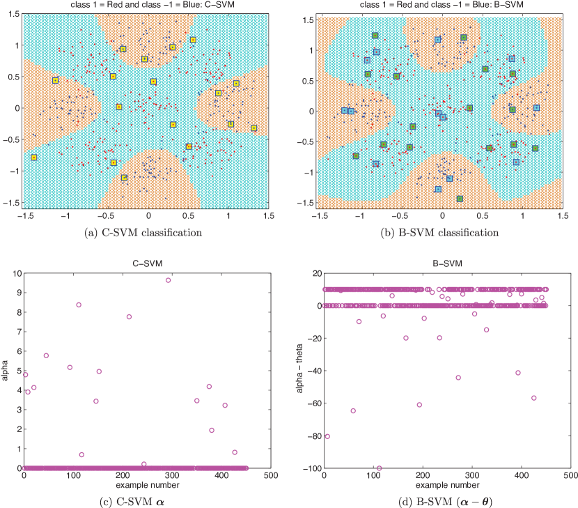
Figure 2: Figure shows classification obtained for example data using (a) C-SVM and (b) B-SVM. Red and Blue points (.) correspond to class $+1$ and $-1$ respectively. Cyan and Orange x-marks (x) show the C-SVM and B-SVM decision rules evaluated at various points. Class $1$ membership is indicated in Cyan and class $-1$ membership is indicated in Orange. The yellow squares in (a) correspond to support points for which $0<\alpha_{i}<C$. The cyan squares in (b) correspond to support points for which $0<\theta_{i}<C_{2}$ and the green squares correspond to support points for which $0<\alpha_{i}<C_{1}$. The sparsity of solution is controlled by $\boldsymbol{\alpha}$ in the case of C-SVM and $(\boldsymbol{\alpha}-\boldsymbol{\theta})$ in the case of B-SVM (c) Shows $\alpha_{i}$ values for C-SVM. (d) Shows $(\alpha_{i}-\theta_{i})$ values for B-SVM.

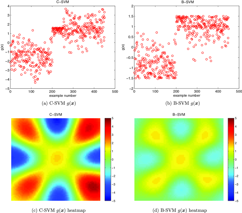
Figure 3: Figure shows decision rule $g(\boldsymbol{x})$ for C-SVM (a) and B-SVM (b). Note that in B-SVM the second penalty term $C_{2}\sum_{i=1}^{n}[y_{i}(\boldsymbol{\beta}^{T}\boldsymbol{h}(\boldsymbol{x_{i}})+\beta_{0})-\rho_{2}]_{+}$ results in most of the $g(\boldsymbol{x})$ values in the interval $[\rho_{1},\rho_{2}]=[1,1.5]$. (c) Heat map of the decision rule $g(\boldsymbol{x})$ for C-SVM (d) Heat map of the decision rule $g(\boldsymbol{x})$ for B-SVM. In C-SVM the values of decision rule $g(\boldsymbol{x})$ are unbalanced in Class $1$. The central cluster located at $(0,0)$ in Class $1$ gets much smaller $g(\boldsymbol{x})$ values in C-SVM than the rest of the Class $1$. In B-SVM however, all clusters in Class $1$ including the one centered at $(0,0)$ get similar $g(\boldsymbol{x})$ values. This is a result of the second penalty term in the B-SVM objective function.

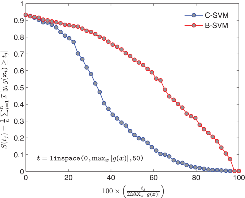
Figure 4: Figure shows the fraction of points classified correctly by both C-SVM (blue curve) and B-SVM (red curve) as a function of the decision rule threshold. The $x$-axis shows the decision rule threshold as a percentage of the maximum absolute value of the decision function $g(\boldsymbol{x})$ over all training points. The $y$-axis shows the overall classification accuracy or sensitivity of C-SVM and B-SVM.

Both C-SVM and B-SVM were fitted to the toy data described above. The following differences in the two solutions are noteworthy:

4.1 $\alpha$-SVs and $\theta$-SVs

The B-SVM dual problem 3.14 contains two variables $\boldsymbol{\alpha}$ and $\boldsymbol{\theta}$. Both $\alpha_{i}$ and $\theta_{i}$ are positive and satisfy the bound constraints given in 3.14. Therefore, similar to C-SVM, we define 2 types of support vectors (SVs) in B-SVM:

• Points $i$ for which $\theta_{i}>0$ are called the $\theta$-SVs     🖘  new SVs that arise in B-SVM

• Points $i$ for which $\alpha_{i}>0$ are called the $\alpha$-SVs     🖘  standard C-SVM like SVs

Figures 2(a) and 2(b) show the C-SVM and B-SVM induced classification respectively for this example problem. Figure 2(b) shows $\alpha$-SVs for which $0<\alpha_{i}<C_{1}$ and $\theta$-SVs for which $0<\theta_{i}<C_{2}$. It is clear from 3.19 that the sparsity of a B-SVM decision rule depends on the quantities $(\alpha_{i}-\theta_{i})$. Figures 2(c) and 2(d) show a plot of $\alpha_{i}$ for C-SVM and $(\alpha_{i}-\theta_{i})$ for B-SVM respectively.

4.2 Bounded decision rule

Figures 3(a) and 3(b) show the decision rule values $g(\boldsymbol{x})$ over all training points for C-SVM and B-SVM. Recall that C-SVM does not enforce an upper limit on $g(\boldsymbol{x})$ whereas B-SVM attempts to encourage $g(\boldsymbol{x})$ to lie in $[\rho_{1},\rho_{2}]$. It can be seen in Figure 3(b) that B-SVM was successful in limiting the absolute value of $g(\boldsymbol{x})$ to be $<\rho_{2}=1.5$ with $C_{2}=100$. Figures 3(c) and 3(d) show a heat map of the decision rule for C-SVM and B-SVM respectively evaluated over a 2-D grid containing the training points. It can be seen that:

• The C-SVM decision rule values are unbalanced in class $+1$ as the central cluster in class $+1$ gets lower $g(\boldsymbol{x})$ values compared to other clusters in class $+1$.

• The decision rule values are balanced in class $+1$ for B-SVM.

4.3 Sensitivity curve

We calculate the quantity:

$$S(t)=\frac{1}{n}\sum_{i=1}^{n}\mathcal{I}\left[y_{i}\,g(\boldsymbol{x_{i}})\geq t\right]$$ (4.2)

which is simply the fraction of correctly classified points (or sensitivity) using decision rule $g(\boldsymbol{x})$ at threshold $t$. To illustrate the variation in sensitivity of C-SVM and B-SVM decision rules:

• For both C-SVM and B-SVM, we divide the range of $g(\boldsymbol{x})$ into $50$ equally spaced points as follows (in MATLAB notation):

  $$\boldsymbol{t}=\verb+linspace(0,+\mbox{max}_{\boldsymbol{x}}\,|g(\boldsymbol{x})|\verb+,50)+$$ (4.3)

• Then we plot $100\times\left(\frac{t_{j}}{\mbox{max}_{\boldsymbol{x}}\,|g(\boldsymbol{x})|}\right)$ versus $S(t_{j})$.

Figure 4 shows this sensitivity curve. It can be seen that for the same percentage threshold on the decision rule range:

• B-SVM has higher classification accuracy (or is more sensitive) than C-SVM.

• This effect is because of the balanced nature of decision rule values in B-SVM compared to C-SVM (see Figure 3(c) and 3(d)).

5 Discussion and conclusions

In this work, we considered the binary classification problem when the feature vectors in individual classes have finite co-variance. We showed that B-SVM is a natural generalization to C-SVM in this situation. It turns out that the B-SVM dual maximization problem 3.14 retains the concavity property of its C-SVM counterpart and C-SVM turns out to be a special case of B-SVM when $C_{2}=0$. Two types of SVs arise in B-SVM, the $\alpha$-SVs which are similar to the standard SVs in C-SVM and $\theta$-SVs which arise due to the novel B-SVM objective function penalty 2.3. The B-SVM decision rule is more balanced than the C-SVM decision rule since it assigns $g(\boldsymbol{x})$ values that are comparable in magnitude to different sub-classes (or clusters) of class $+1$ and class $-1$. In addition, B-SVM retains higher classification accuracy compared to C-SVM as the decision rule threshold is varied from $0$ to $\mbox{max}_{\boldsymbol{x}}\,|g(\boldsymbol{x})|$. For a training set of size $n$, B-SVM results in a dual optimization problem of size $2n$ compared to a C-SVM dual problem of size $n$. Hence it is computationally more expensive to solve a B-SVM problem.

In summary, B-SVM can be used to enforce balanced decision rules in binary classification. It is anticipated that the C-SVM leave one out error bounds for the bias free case given in Jaakkola and Haussler (1999) will continue to hold in a similar form for bias free B-SVM as well.

References

- Boser et al. [1992] B. E. Boser, I. M. Guyon, and V. N. Vapnik. A training algorithm for optimal margin classifiers. In Proceedings of the fifth annual workshop on Computational learning theory, COLT ’92, pages 144–152, 1992.
- Cortes and Vapnik [1995] C. Cortes and V. Vapnik. Support-vector networks. Machine Learning, 20:273–297, 1995.
- Jaakkola and Haussler [1999] T. S. Jaakkola and D. Haussler. Probabilistic kernel regression models. In Proceedings of the 1999 Conference on AI and Statistics, 1999.
- Nocedal and Wright [2006] J. Nocedal and S. J Wright. Numerical Optimization, 2nd Edition. New York-Springer, 2006.
- Platt [1998] J. C. Platt. Fast training of support vector machines using sequential minimal optimization. In B. Schoelkopf, C. Burges, and A. Smola, editors, Advances in Kernel Methods - Support Vector Learning. MIT Press, 1998.
- Vapnik and Lerner [1963] V. Vapnik and A. Lerner. Pattern recognition using generalized portrait method. Automation and Remote Control, 24:774–780, 1963.