Blending Bayesian and frequentist methods according to the precision of prior information with an application to hypothesis testing
 

Abstract

The following zero-sum game between nature and a statistician blends Bayesian methods with frequentist methods such as p-values and confidence intervals. Nature chooses a posterior distribution consistent with a set of possible priors. At the same time, the statistician selects a parameter distribution for inference with the goal of maximizing the minimum Kullback-Leibler information gained over a confidence distribution or other benchmark distribution. An application to testing a simple null hypothesis leads the statistician to report a posterior probability of the hypothesis that is informed by both Bayesian and frequentist methodology, each weighted according how well the prior is known.

As is generally acknowledged, the Bayesian approach is ideal given knowledge of a prior distribution that can be interpreted in terms of relative frequencies. On the other hand, frequentist methods such as confidence intervals and p-values have the advantage that they perform well without knowledge of such a distribution of the parameters. Since neither the Bayesian approach nor the frequentist approach is entirely satisfactory in situations involving partial knowledge of the prior distribution, the proposed procedure reduces to a Bayesian method given complete knowledge of the prior, to a frequentist method given complete ignorance about the prior, and to a blend between the two methods given partial knowledge of the prior. The blended approach resembles the Bayesian method rather than the frequentist method to the precise extent that the prior is known.

The problem of testing a point null hypothesis illustrates the proposed framework. The blended probability that the null hypothesis is true is equal to the p-value or a lower bound of an unknown Bayesian posterior probability, whichever is greater. Thus, given total ignorance represented by a lower bound of 0, the p-value is used instead of any Bayesian posterior probability. At the opposite extreme of a known prior, the p-value is ignored. In the intermediate case, the possible Bayesian posterior probability that is closest to the p-value is used for inference. Thus, both the Bayesian method and the frequentist method influence the inferences made.

David R. Bickel

Ottawa Institute of Systems Biology
Department of Biochemistry, Microbiology, and Immunology
University of Ottawa; 451 Smyth Road; Ottawa, Ontario, K1H 8M5

Keywords: blended inference; confidence distribution; confidence posterior; hybrid inference; maximum entropy; maxmin expected utility; minimum cross entropy; minimum divergence; minimum information for discrimination; minimum relative entropy; observed confidence level; robust Bayesian analysis

1 Introduction

1.1 Motivation

Various compromises between Bayesian and frequentist approaches to statistical inference represent first attempts to combining attractive aspects of each approach (Good, 1983). While the more recent the hybrid inference approach of Yuan (2009) succeeded in leveraging Bayesian point estimators with maximum likelihood estimates, reducing to the former or the latter in the presence or absence of a reliably estimated prior on all parameters, how to extend the theory beyond point estimation is not yet clear. Further, hybrid inference in its current form does not cover the case of a parameter of interest that has a partially known prior. Since such partial knowledge of a prior occurs in many scientific inference situations, it calls for a theoretical framework for method development that appropriately blends Bayesian and frequentist methods.

Ideally, blended inference would meet these criteria:

1. Complete knowledge of the prior. If the prior is known, the corresponding posterior is used for inference. Among statisticians, this principle is almost universally acknowledged. However, it is rarely the case of the prior is known for all practical purposes.

2. Negligible knowledge of the prior. If there is no reliable knowledge of a prior, inference is based on methods that do not require such knowledge. This principle motivates not only the development of confidence intervals and p-values but also Bayesian posteriors derived from improper and data-dependent priors. Accordingly, blended inference must allow the use of such methods when applicable.

3. Continuum between extremes. Inference relies on the prior to the extent that it is known while relying on the other methods to the extent that it is not known. Thus, there is a gradation of methodology between the above two extremes. The premise of this paper is that this intermediate scenario calls for a careful balance between pure Bayesian methods on one hand and impure Bayesian or non-Bayesian methods on the other hand.

Instead of framing the knowledge of a prior in terms of confidence intervals, as in pure empirical Bayes approaches, it will be framed more generally herein in terms of a set of plausible priors, as in interval probability (Weichselberger, 2000; Augustin, 2002, 2004) and robust Bayesian (Berger, 1984) approaches. Whereas the concept of an unknown prior cannot arise in strict Bayesian statistics, it does arise in robust Bayesian statistics when the levels of belief of an intelligent agent have not been fully assessed (Berger, 1984). Unknown priors also occur in many more objective contexts involving purely frequentist interpretations of probability in terms of variability in the observable world rather than the uncertainty in the mind of an agent. For example, frequency-based priors are routinely estimated under random effects and empirical Bayes models; see, e.g., Efron (2010). (Remark 1 comments further on interpretations of probability and relaxes the convenient assumption of a true prior.)

With respect to the problem at hand, the most relevant robust Bayesian approaches are the minimax Bayes risk (“$\Gamma$-minimax”) practice of minimizing the maximum Bayes risk (Robbins, 1951; Berger, 1985; Vidakovic, 2000) and the maxmin expected utility (“conditional $\Gamma$-minimax”) practice of maximizing the minimum posterior expected payoff or, equivalently, minimizing the maximum posterior expected loss (Gilboa and Schmeidler, 1989; DasGupta and Studden, 1989; Vidakovic, 2000; Augustin, 2002, 2004). Augustin (2004) reviews both methods in terms of interval probabilities that need not be subjective. With typical loss functions, the former method meets the above criteria for classical minimax alternatives to Bayesian methods but does not apply to other attractive alternatives. For example, several confidence intervals, p-values, and objective-Bayes posteriors routinely used in biostatistics are not minimax optimal. (Fraser and Reid (1990) and Fraser (2004) argued that requiring the optimality of frequentist procedures can lead to trade-offs between hypothetical samples that potentially mislead scientists or yield pathological procedures.) Optimality in the classical sense is not required of the alternative procedures under the framework outlined below, which can be understood in terms of maxmin expected utility with a payoff function that incorporates the alternative procedures to be used as a benchmark for the Bayesian posteriors.

1.2 Heuristic overview

To define a general theory of blended inference that meets a formal statement of the three criteria, Section 2 introduces a variation of a zero-sum game of Topsøe (1979), Harremoës and Topsøe (2001), and Topsøe (2007). (The discrete version of the game also appeared in Pfaffelhuber (1977), and Grünwald and Philip Dawid (2004) interpreted it as a special case of the maxmin expected utility problem.) The “nature” opponent selects a prior consistent with the available knowledge as the “statistician” player selects a posterior distribution with the aim of maximizing the minimum information gained relative to one or more alternative methods. Such benchmark methods may be confidence interval procedures, frequentist hypothesis tests, or other techniques that are not necessarily Bayesian.

From that theory, Section 3 derives a widely applicable framework for testing hypotheses. For concreteness, the motivating results are heuristically summarized here. Consider the problem of testing $H_{0}:\theta_{\ast}=0$, the hypothesis that a real-valued parameter $\theta_{\ast}$ of interest is equal to the point 0 on the real line $\mathbb{R}$. The observed data vector $x$ is modeled as a realization of a random variable denoted by $X$. Let $p\left(x\right)$ denote the p-value resulting from a statistical test.

It has long been recognized that the p-value for a simple (point) null hypothesis is often smaller than Bayesian posterior probabilities of the hypothesis (Lindley, 1957; Berger and Sellke, 1987). Suppose $\theta_{\ast}$ has an unknown prior distribution according to which the prior probability of $H_{0}$ is $\pi_{0}$. While $\pi_{0}$ is unknown, it is assumed to be no less than some known lower bound denoted by $\underline{\pi}_{0}$.

Following the methodology of Berger et al. (1994), Sellke et al. (2001) found a generally applicable lower bound on the Bayes factor. As Section 3.1 will explain, that bound immediately leads to

$$\underline{\Pr}\left(H_{0}|p\left(X\right)=p\left(x\right)\right)=\left(1-\left(\frac{1-\underline{\pi}_{0}}{\underline{\pi}_{0}ep\left(x\right)\log p\left(x\right)}\right)\right)^{-1}$$ (1)

as a lower bound on the unknown posterior probability of the null hypothesis for $p\left(x\right)<1/e$ and to $\underline{\pi}_{0}$ as a lower bound on the probability if $p\left(x\right)\geq 1/e$.

In addition to $\Pr\left(H_{0}|p\left(X\right)=p\left(x\right)\right),$ the unknown Bayesian posterior probability of $H_{0}$, there is a frequentist posterior probability of $H_{0}$ that will guide selection of a posterior probability for inference based on $\pi_{0}\geq\underline{\pi}_{0}$ and other constraints summarized by $\Pr\left(H_{0}|p\left(X\right)=p\left(x\right)\right)\geq\underline{\Pr}\left(H_{0}|p\left(X\right)=p\left(x\right)\right)$. While it is incorrect to interpret the p-value $p\left(x\right)$ as a Bayesian probability, it will be seen in Section 3.2 that $p\left(x\right)$ is a confidence posterior probability that $H_{0}$ is true.

With the confidence posterior as the benchmark, the solution to the optimization problem described above gives the blended posterior probability that the null hypothesis is true. It is simply the maximum of the p-value and the lower bound on the Bayesian posterior probability:

$$\Pr\left(H_{0};p\left(x\right)\right)=p\left(x\right)\vee\underline{\Pr}\left(H_{0}|p\left(X\right)=p\left(x\right)\right).$$ (2)

By plotting $\Pr\left(H_{0};p\left(x\right)\right)$ as a function of $p\left(x\right)$ and $\underline{\pi}_{0}$, Figures 1 and 2 illustrate each of the above criteria for blended inference:

1. Complete knowledge of the prior. In this example, the prior is only known when $\underline{\pi}_{0}=1$, in which case

   $$\Pr\left(H_{0};p\left(x\right)\right)=\underline{\Pr}\left(H_{0}|p\left(X\right)=p\left(x\right)\right)=1$$

   for all $p\left(x\right)$. Thus, the p-value is ignored in the presence of a known prior.

2. Negligible knowledge of the prior. There is no knowledge of the prior when $\underline{\pi}_{0}=0$ and negligible knowledge when $\underline{\pi}_{0}$ is so low that $\underline{\Pr}\left(H_{0}|p\left(X\right)=p\left(x\right)\right)\leq p\left(x\right)$. In such cases, $\Pr\left(H_{0};p\left(x\right)\right)=p\left(x\right)$, and the Bayesian posteriors are ignored.

3. Continuum between extremes. When $\underline{\pi}_{0}$ is of intermediate value in the sense that $\underline{\Pr}\left(H_{0}|p\left(X\right)=p\left(x\right)\right)$ is exclusively between $p\left(x\right)$ and 1,

   $$\Pr\left(H_{0};p\left(x\right)\right)=\underline{\Pr}\left(H_{0}|p\left(X\right)=p\left(x\right)\right)<1.$$

   Consequently, $\Pr\left(H_{0};p\left(x\right)\right)$ increases gradually from $p\left(x\right)$ to 1 as $\underline{\pi}_{0}$ increases (Figures 1 and 2). In this case, the blended posterior lies in the set of allowed Bayesian posteriors but is on the boundary of that set that is the closest to the p-value. Thus, both the p-value and the Bayesian posteriors influence the blended posterior and thus the inferences made on its basis.

The plotted parameter distribution will be presented in Section 3.3 as a widely applicable blended posterior.

Finally, Section 4 offers additional details and generalizations in a series of remarks.

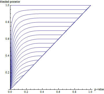
Figure 1: Blended posterior probability that the null hypothesis is true versus the p-value. The curves correspond to lower bounds of prior probabilities ranging in 5% increments from 0% on the bottom to 100% on the top.

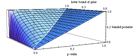
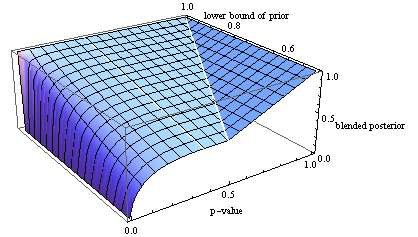
Figure 2: Blended posterior probability that the null hypothesis is true versus the p-value and the lower bound of the prior probability that the null hypothesis is true. The top plot displays the full domain, half of which is shown in the bottom plot.

2 General theory

2.1 Preliminary notation and definitions

Denote the observed data set, typically a vector or matrix of observations, by $x$, a member of a set $\mathcal{X}$ that is endowed with a $\sigma$-algebra $\mathfrak{X}$. The value of $x$ determines two sets of posterior distributions that can be blended for inference about the value of a target parameter. Much of the following notation is needed to transform general Bayesian posteriors and confidence posteriors or other benchmark posteriors such that they are defined on the same measurable space, that of the target parameter. (A confidence posterior, to be defined in Section 3.2.1, is a parameter distribution from which confidence intervals and p-values may be extracted. As such, it facilitates blending typical frequentist procedures with Bayesian procedures.)

2.1.1 Bayesian posteriors

With some measurable space $\left(\dot{\Theta}_{\ast},\dot{\mathcal{A}}_{\ast}\right)$ for parameter values in $\dot{\Theta}_{\ast}$, let $\mathcal{P}_{\ast}^{\operatorname{prior}}$ denote a set of probability distributions on $\left(\mathcal{X}\times\dot{\Theta}_{\ast},\mathfrak{X}\otimes\dot{\mathcal{A}}_{\ast}\right)$. Any distribution in $\mathcal{P}_{\ast}^{\operatorname{prior}}$ is called a prior (distribution), understood in the broad sense of a model that includes the possible likelihood functions as well as the parameter distribution. It encodes the constraints and other information available about the parameter before observing $x$.

On the other hand, any distribution of a parameter is called a posterior (distribution) if it depends on $x$. For some $P_{\ast}^{\operatorname{prior}}\in\mathcal{P}_{\ast}^{\operatorname{prior}}$, an example of a posterior distribution on $\left(\dot{\Theta}_{\ast},\dot{\mathcal{A}}_{\ast}\right)$ is $\dot{P}_{\ast}=P_{\ast}^{\operatorname{prior}}\left(\bullet|X=x\right)$, where $X$ is a random variable of a distribution on $\left(\mathcal{X},\mathfrak{X}\right)$ that is determined by $P_{\ast}^{\operatorname{prior}}$. $\dot{P}_{\ast}$ is called a Bayesian posterior (distribution) since it is equal to a conditional distribution of the parameter given $X=x$. Adapting an apt term from Topsøe (2007), the set $\dot{\mathcal{P}}_{\ast}=\left\{P_{\ast}^{\operatorname{prior}}\left(\bullet|X=x\right):P_{\ast}^{\operatorname{prior}}\in\mathcal{P}_{\ast}^{\operatorname{prior}}\right\}$ of Bayesian posteriors on $\left(\dot{\Theta}_{\ast},\dot{\mathcal{A}}_{\ast}\right)$ may be considered the “knowledge base.” For a set $\dot{\Theta}$, if $\dot{\tau}:\dot{\Theta}_{\ast}\rightarrow\Theta$ is an $\dot{\mathcal{A}}_{\ast}$-measurable map and if $\dot{\theta}_{\ast}$ has distribution $\dot{P}_{\ast}\in\dot{\mathcal{P}}_{\ast}$, then $\dot{\theta}=\dot{\tau}\left(\dot{\theta}_{\ast}\right)$, referred to as an inferential target of $\dot{P}_{\ast}$, has induced probability space $\left(\Theta,\mathcal{A},\dot{P}\right)$. The set

$$\dot{\mathcal{P}}=\left\{\dot{P}:\dot{\tau}\left(\dot{\theta}_{\ast}\right)\sim\dot{P},\dot{\theta}_{\ast}\sim\dot{P}_{\ast}\in\dot{\mathcal{P}}_{\ast}\right\}$$

of all distributions thereby induced and the set $\mathcal{P}$ of all probability distributions on $\left(\Theta,\mathcal{A}\right)$ are related by $\dot{\mathcal{P}}\subseteq\mathcal{P}$.

Example 1.

In the hypothesis test of Section 1.2, $\dot{\theta}=0$ if the null hypothesis that $\dot{\theta}_{\ast}=0$ is true and $\dot{\theta}=1$ if the alternative hypothesis that $\dot{\theta}_{\ast}\neq 0$ is true, where $\dot{\theta}_{\ast}$ and $\dot{\theta}$ are random variables with distributions respectively defined on the Borel space $\left(\mathbb{R},\mathcal{B}\left(\mathbb{R}\right)\right)$ and the discrete space $\left(\left\{0,1\right\},2^{\left\{0,1\right\}}\right)$, where $2^{\left\{0,1\right\}}$ is the power set of $\left\{0,1\right\}$. Thus, in this case, $\dot{\tau}$ is the indicator function $1_{\left(-\infty,0\right)\cup\left(0,\infty\right)}:\mathbb{R}\rightarrow\left\{0,1\right\}$, yielding $\dot{\theta}=1_{\left(-\infty,0\right)\cup\left(0,\infty\right)}\left(\dot{\theta}_{\ast}\right)$. Section 3 considers this example in more detail.

A function that transforms a set of parameter distributions to a single parameter distribution on the same measurable space is called an inference process (Paris, 1994; Paris and Vencovská, 1997). The resulting distribution is known as a “representation” (Augustin, 2002) or “reduction” (Bickel, 2011a) of the set. Perhaps the best known inference process for a discrete parameter set $\Theta$ is that of the maximum entropy principle, which would select a member of $\dot{\mathcal{P}}$ such that it has higher entropy than any other member of the set (see Remark 2). This paper will propose a wide class of inference processes such that each transforms $\dot{\mathcal{P}}$ to a member of $\mathcal{P}$ on the basis the following concept of a benchmark distribution on $\left(\Theta,\mathcal{A}\right)$.

2.1.2 Benchmark posteriors

For the convenience of the reader, the same Latin and Greek letters will be used for the set of posteriors that will represent a gold standard or benchmark method of inference as for the Bayesian posteriors of Section 2.1.1, with the double-dot $\ddot{\bullet}$ replacing the single-dot $\dot{\bullet}$. Let $\ddot{\mathcal{P}}_{\ast}$ represent a set of posterior distributions on some measurable space $\left(\ddot{\Theta}_{\ast},\ddot{\mathcal{A}}_{\ast}\right)$, and let $\ddot{\mathfrak{P}}_{\ast}$ represent a set of such sets. For instance, considering any $\ddot{P}_{\ast}$ in $\ddot{\mathcal{P}}_{\ast}$, $\ddot{P}_{\ast}$ may be a confidence posterior (a fiducial-like distribution to be defined precisely in Section 3.2), a generalized fiducial posterior of Hannig (2009), or even a Bayesian posterior based on an improper prior. (In the first case, nested confidence intervals with inexact coverage rates generate a set $\ddot{\mathcal{P}}_{\ast}$ of multiple confidence posteriors rather than the single confidence posterior that is generated by exact confidence intervals (Bickel, 2011a).) Suppose there exists a function $\boldsymbol{\ddot{\tau}}:\ddot{\mathfrak{P}}_{\ast}\rightarrow\Theta$ such that $\ddot{P}$, the probability distribution of $\boldsymbol{\ddot{\tau}}\left(\ddot{\mathcal{P}}_{\ast}\right)$, is defined on $\left(\Theta,\mathcal{A}\right)$. $\ddot{P}$ is called the benchmark posterior (distribution), and $\ddot{\theta}=\boldsymbol{\ddot{\tau}}\left(\ddot{\mathcal{P}}_{\ast}\right)$ is the inferential target of $\ddot{\mathcal{P}}_{\ast}$. It follows that $\ddot{P}$ is in $\mathcal{P}$ but not necessarily in $\dot{\mathcal{P}}$.

Example 2.

Consider a model in which the full parameter $\dot{\theta}_{\ast}\in\dot{\Theta}_{\ast}$ consists of an interest parameter $\dot{\theta}$ and a nuisance parameter $\dot{\lambda}$. The measurable space of $\dot{\theta}_{\ast}=\left\langle\dot{\theta},\dot{\lambda}\right\rangle$ is denoted by $\left(\dot{\Theta}_{\ast},\dot{\mathcal{A}}_{\ast}\right)$, and that of $\dot{\theta}$ by $\left(\Theta,\mathcal{A}\right)$. Suppose that a set of Bayesian posteriors is available for $\dot{\theta}_{\ast}$ but that nested confidence intervals are only available for an unknown parameter $\theta\in\Theta$. It follows that a confidence posterior $\ddot{P}$ is available on $\left(\Theta,\mathcal{A}\right)$ but not on $\left(\dot{\Theta}_{\ast},\dot{\mathcal{A}}_{\ast}\right)$. Then the framework of this section can be applied by using the function $\dot{\tau}$ such that $\theta=\dot{\tau}\left(\dot{\theta}_{\ast}\right)$ in order to project the Bayesian posteriors onto $\left(\Theta,\mathcal{A}\right)$, the measurable space on which $\ddot{P}$ is defined. In this case, since there is only one possible benchmark posterior, the function $\boldsymbol{\ddot{\tau}}$ need not be explicitly constructed.

The function $\boldsymbol{\ddot{\tau}}$ allows consideration of a set of possible benchmark posteriors by transforming it to a single benchmark posterior defined on $\left(\Theta,\mathcal{A}\right)$, the same measurable space as the above Bayesian posteriors of $\dot{\theta}$. Since that function is unusual, two ways to compose it will now be explained.

Example 3.

Consider the inference process $\ddot{\Pi}:\ddot{\mathfrak{P}}_{\ast}\rightarrow\mathcal{P}_{\ast}$, where $\mathcal{P}_{\ast}$ is the set of all probability distributions on $\left(\ddot{\Theta}_{\ast},\ddot{\mathcal{A}}_{\ast}\right)$. Define the random variable $\ddot{\theta}_{\ast}$ to have distribution $\ddot{\Pi}\left(\ddot{\mathcal{P}}_{\ast}\right)\left(\bullet\right)=\ddot{\Pi}\left(\ddot{\mathcal{P}}_{\ast}\right)$. If $\ddot{\tau}:\ddot{\Theta}_{\ast}\rightarrow\Theta$ is an $\ddot{\mathcal{A}}_{\ast}$-measurable function, then $\ddot{\theta}=\ddot{\tau}\left(\ddot{\theta}_{\ast}\right)$ is the inferential target of $\ddot{\mathcal{P}}_{\ast}$. Further, the distribution $\ddot{P}$ of $\ddot{\theta}$ is the benchmark posterior.

Example 4.

Whereas Example 3 applied an inference process before a parameter transformation, this example reverses the order by first applying $\ddot{\tau}$. Let $\ddot{\mathcal{P}}$ denote the subset of $\mathcal{P}$ consisting of all distributions of the parameters transformed by $\ddot{\tau}$:

$$\ddot{\mathcal{P}}=\left\{P:\ddot{\tau}\left(\ddot{\theta}_{\ast}\right)\sim P,\ddot{\theta}_{\ast}\sim\ddot{P}_{\ast}\in\ddot{\mathcal{P}}_{\ast}\right\}.$$

Then an inference process transforms $\ddot{\mathcal{P}}$ to the benchmark posterior $\ddot{P}$, which in turn is the distribution of $\ddot{\theta}$, the inferential target of $\ddot{\mathcal{P}}_{\ast}$.

2.2 Blended inference

In terms of Radon-Nikodym differentiation, the information divergence of $P$ with respect to $Q$ on $\left(\Theta,\mathcal{A}\right)$ is

$$I\left(P||Q\right)=\int dP\log\left(\frac{dP}{dQ}\right)$$ (3)

if $P\ll Q$ and $I\left(P||Q\right)=\infty$ otherwise. $I\left(P||Q\right)$ is also known as cross/relative entropy, $I$-divergence, information for discrimination, and Kullback-Leibler divergence. Other measures of information may also be used (Remark 3). For any posteriors $\dot{P}\in\dot{\mathcal{P}}$ and $Q\in\mathcal{P}$, the inferential gain $I\left(\dot{P}||\ddot{P}\rightsquigarrow Q\right)$ of $Q$ relative to $\ddot{P}$ given $\dot{P}$ is the amount of information gained by making inferences on the basis of $Q$ instead of the benchmark posterior $\ddot{P}$:

$$I\left(\dot{P}||\ddot{P}\rightsquigarrow Q\right)=I\left(\dot{P}||\ddot{P}\right)-I\left(\dot{P}||Q\right).$$

Let $\dot{\mathcal{P}}\left(\ddot{P}\right)$ denote the largest subset of $\dot{\mathcal{P}}$ such that the information divergence of any of its members with respect to $\ddot{P}$ is finite. That is,

$$\dot{\mathcal{P}}\left(\ddot{P}\right)=\left\{\dot{P}\in\dot{\mathcal{P}}:I\left(\dot{P}||\ddot{P}\right)<\infty\right\},$$ (4)

which is nonempty by assumption. (The assumption is not necessary under the generalization described in Remark 4.)

The blended posterior (distribution) $\hat{P}$ is the probability distribution on $\left(\Theta,\mathcal{A}\right)$ that maximizes the inferential gain relative to the benchmark posterior given the worst-case posterior restricted by the constraints that defined $\dot{\mathcal{P}}$ and $\dot{\mathcal{P}}\left(\ddot{P}\right)$:

$$\inf_{\dot{P}\in\dot{\mathcal{P}}\left(\ddot{P}\right)}I\left(\dot{P}||\ddot{P}\rightsquigarrow\hat{P}\right)=\sup_{Q\in\mathcal{P}}\inf_{\dot{P}\in\dot{\mathcal{P}}\left(\ddot{P}\right)}I\left(\dot{P}||\ddot{P}\rightsquigarrow Q\right),$$ (5)

where the supremum and infinum over any set including an indeterminate number are $\infty$ and $-\infty$, respectively (Topsøe, 2007). Inferences based on $\hat{P}$ are blended in the sense that they depend on both $\dot{\mathcal{P}}$ and $\ddot{P}$ in the ways to be specified in Section 2.3.

The main result of Theorem 2 of Topsøe (2007) gives a simply stated solution of the optimality problem of equation (5) under broad conditions.

Proposition 1.

If $I\left(\dot{P}||\ddot{P}\right)<\infty$ for some $\dot{P}\in\dot{\mathcal{P}}$ and if $\dot{\mathcal{P}}\left(\ddot{P}\right)$ is convex, then the blended posterior $\hat{P}$ is the probability distribution in $\dot{\mathcal{P}}$ that minimizes the information divergence with respect to the benchmark posterior:

$$I\left(\hat{P}||\ddot{P}\right)=\inf_{\dot{P}\in\dot{\mathcal{P}}\left(\ddot{P}\right)}I\left(\dot{P}||\ddot{P}\right).$$ (6)

Proof.

Topsøe (2007) proved the result from inequalities of information theory given the additional stated condition of his Theorem 2 that $I\left(\dot{P}||\ddot{P}\right)<\infty$ for all $\dot{P}\in\dot{\mathcal{P}}\left(\ddot{P}\right)$. (See Remark 4.) The condition that $I\left(\dot{P}||\ddot{P}\right)<\infty$ for some $\dot{P}\in\dot{\mathcal{P}}$ and the above definition of $\dot{\mathcal{P}}\left(\ddot{P}\right)$ ensure that the condition is met. ∎

Alternatively, the minimization of information divergence may define $\hat{P}$ rather than result from its definition in terms of the game (Remark 5).

2.3 Properties of blended inference

The desiderata of Section 1 for blended inference can now be formalized. A posterior distribution $\tilde{P}\left(\bullet;\dot{\mathcal{P}},\ddot{P}\right)$ on $\left(\Theta,\mathcal{A}\right)$ is said to blend the set $\dot{\mathcal{P}}$ of Bayesian posteriors with the benchmark posterior $\ddot{P}$ for inference about the parameter in $\Theta$ provided that $\tilde{P}\left(\bullet;\dot{\mathcal{P}},\ddot{P}\right)$ satisfies the following criteria under the conditions of Proposition 1:

1. Complete knowledge of the prior. If $\dot{\mathcal{P}}$ has a single member $\dot{P}$, then $\tilde{P}\left(\bullet;\dot{\mathcal{P}},\ddot{P}\right)=\dot{P}$.

2. Negligible knowledge of the prior. If $\ddot{P}\in\dot{\mathcal{P}}$ and if $\dot{\mathcal{P}}$ has at least two members, then $\tilde{P}\left(\bullet;\dot{\mathcal{P}},\ddot{P}\right)=\ddot{P}$.

3. Continuum between extremes. For any $D\geq 0$ and any $\mathcal{P}^{\star}\subseteq\mathcal{P}$ such that

   $$\sup_{P\in\mathcal{P}^{\star},\dot{P}\in\dot{\mathcal{P}}\left(\ddot{P}\right)}\left|I\left(P||\ddot{P}\right)-I\left(\dot{P}||\ddot{P}\right)\right|\leq D$$ (7)

   and such that $\dot{\mathcal{P}}\left(\ddot{P}\right)\cup\mathcal{P}^{\star}$ is convex,

   $$\left|I\left(\tilde{P}\left(\bullet;\dot{\mathcal{P}}\cup\mathcal{P}^{\star},\ddot{P}\right)||\ddot{P}\right)-I\left(\tilde{P}\left(\bullet;\dot{\mathcal{P}},\ddot{P}\right)||\ddot{P}\right)\right|\leq D.$$ (8)

Theorem 1.

The blended posterior $\hat{P}$ blends the set $\dot{\mathcal{P}}$ of Bayesian posteriors with the benchmark posterior $\ddot{P}$ for inference about the parameter in $\Theta$.

Proof.

Since the criteria are only required under the conditions of Proposition 1, it will suffice to prove that the criteria follow from equation (6). If $\dot{\mathcal{P}}$ has a single member $\dot{P}$, then equation (6) implies that $\hat{P}=\dot{P}$, thereby ensuring Criterion 1. Similarly, if $\ddot{P}\in\dot{\mathcal{P}}$, then equation (6) implies that $\hat{P}=\ddot{P}$, thus proving that Criterion 2 is met. Assume, contrary to Criterion 3, that there exist a $D\geq 0$ and a $\mathcal{P}^{\star}\subseteq\mathcal{P}$ such that $\dot{\mathcal{P}}\left(\ddot{P}\right)\cup\mathcal{P}^{\star}$ is convex, equation (7) is true, and equation (8) is false with $\tilde{P}\left(\bullet;\dot{\mathcal{P}}\cup\mathcal{P}^{\star},\ddot{P}\right)$ and $\tilde{P}\left(\bullet;\dot{\mathcal{P}},\ddot{P}\right)$ equal to the blended posteriors respectively using $\dot{\mathcal{P}}\cup\mathcal{P}^{\star}$ and $\dot{\mathcal{P}}$ as the sets of Bayesian posteriors. Then equation (6) can be written as

$$I\left(\tilde{P}\left(\bullet;\dot{\mathcal{P}}\cup\mathcal{P}^{\star},\ddot{P}\right)||\ddot{P}\right)=\inf_{\dot{P}\in\dot{\mathcal{P}}\left(\ddot{P}\right)\cup\mathcal{P}^{\star}}I\left(\dot{P}||\ddot{P}\right);$$

$$I\left(\tilde{P}\left(\bullet;\dot{\mathcal{P}},\ddot{P}\right)||\ddot{P}\right)=\inf_{\dot{P}\in\dot{\mathcal{P}}\left(\ddot{P}\right)}I\left(\dot{P}||\ddot{P}\right).$$

Hence, with $a\wedge b$ signifying the minimum of $a$ and $b$,

$$\left|I\left(\tilde{P}\left(\bullet;\dot{\mathcal{P}}\cup\mathcal{P}^{\star},\ddot{P}\right)||\ddot{P}\right)-I\left(\tilde{P}\left(\bullet;\dot{\mathcal{P}},\ddot{P}\right)||\ddot{P}\right)\right|=$$

$$\inf_{\dot{P}\in\dot{\mathcal{P}}\left(\ddot{P}\right)}I\left(\dot{P}||\ddot{P}\right)-\inf_{\dot{P}\in\dot{\mathcal{P}}\left(\ddot{P}\right)}I\left(\dot{P}||\ddot{P}\right)\wedge\inf_{P\in\mathcal{P}^{\star}}I\left(P||\ddot{P}\right),$$

which cannot exceed $\inf_{\dot{P}\in\dot{\mathcal{P}}\left(\ddot{P}\right)}I\left(\dot{P}||\ddot{P}\right)-\inf_{P\in\mathcal{P}^{\star}}I\left(P||\ddot{P}\right)$ and thus, according to equation (7), cannot exceed $D$. Therefore, the above assumption that equation (8) is false is contradicted, thereby establishing satisfaction of Criterion 3. ∎

Example 5.

Suppose the set of possible priors consists of a single frequency-matching prior, i.e., a prior that leads to 95% posterior credible intervals that are equal to 95% confidence intervals, etc. If the benchmark posterior is the confidence posterior that yields the same confidence intervals, then it is the Bayesian posterior distribution corresponding to the prior. In that case, the blended distribution is equal to that Bayesian/confidence posterior. Thus, the first condition of blended inference applies. The second condition would instead apply if the set of possible priors contained at least one other prior in addition to the frequency-matching prior.

Criterion 3 is much stronger than the heuristic idea of continuity introduced in Section 1.1. Its use of information divergence can be generalized to other measures of divergence (Remark 3).

3 Blended hypothesis testing

A fertile field of application for the theory of Section 2 is that of testing hypotheses, as outlined in Section 1.2. Building on Example 1, this section provides methodology for a wide class of models used in hypothesis testing.

3.1 A bound on the Bayesian posterior

Defining that class in terms of the concepts of Section 2.1.1 requires additional notation. For a continuous sample space $\mathcal{X}$ and a function $p:\mathcal{X}\rightarrow\left[0,1\right]$ such that $p\left(X\right)\sim\operatorname{U}\left(0,1\right)$ under a null hypothesis, each $p\left(x\right)$ for any $x\in\mathcal{X}$ will be called a p-value. Using some dominating measure, let $f_{0}$ and $f_{1}$ denote probability density functions of $p\left(X\right)$ under the null hypothesis $\left(\dot{\theta}=0\right)$ and under the alternative hypothesis $\left(\dot{\theta}=1\right)$, respectively. For the observed $x$, the likelihood ratio $f_{0}\left(p\left(x\right)\right)/f_{1}\left(p\left(x\right)\right)$ is called the Bayes factor since, for a prior distribution $P_{\ast}^{\operatorname{prior}}$, Bayes’s theorem gives

$$\frac{\varphi\left(p\left(x\right)\right)}{1-\varphi\left(p\left(x\right)\right)}=\frac{P_{\ast}^{\operatorname{prior}}\left(\dot{\theta}=0\right)}{P_{\ast}^{\operatorname{prior}}\left(\dot{\theta}=1\right)}\frac{f_{0}\left(p\left(x\right)\right)}{f_{1}\left(p\left(x\right)\right)},$$ (9)

where $\varphi\left(p\left(x\right)\right)=P_{\ast}^{\operatorname{prior}}\left(\dot{\theta}=0|p\left(X\right)=p\left(x\right)\right)$. Here, as $\varphi\left(p\left(x\right)\right)$ is a local false discovery rate (LFDR), the letter $\varphi$ abbreviates “false” (Efron, 2010; Bickel, 2011c). In a parametric setting, $f_{1}\left(p\left(x\right)\right)$ would be the likelihood integrated over the prior distribution conditional on the alternative hypothesis.

Let $\kappa:\mathcal{X}\rightarrow\mathbb{R}$ denote the function defined by the transformation $\kappa\left(x\right)=-\log p\left(x\right)$ for all $x\in\mathcal{X}$. Then a probability density of $\kappa\left(X\right)$ under the null hypothesis is the standard exponential density $g_{0}\left(\kappa\left(x\right)\right)=e^{-\kappa\left(x\right)}$. Assume that, under the alternative hypothesis $\left(\dot{\theta}=1\right)$, $\kappa\left(X\right)$ admits a density function $g_{1}$ with respect to the same dominating measure as $g_{0}$. It follows that $g_{0}\left(\kappa\left(x\right)\right)/g_{1}\left(\kappa\left(x\right)\right)=f_{0}\left(p\left(x\right)\right)/f_{1}\left(p\left(x\right)\right)$. The hazard rate $h_{1}\left(\kappa\left(x\right)\right)$ under the alternative is defined by $h_{1}\left(\kappa\left(x\right)\right)=g_{1}\left(\kappa\left(x\right)\right)/\int_{\kappa\left(x\right)}^{\infty}g_{1}\left(k\right)dk$ for all $x\in\mathcal{X}$, and $h_{1}:\left(0,\infty\right)\rightarrow\left[0,\infty\right)$ is called the hazard rate function.

Sellke et al. (2001) obtained the following lower bound $\underline{b}\left(p\left(x\right)\right)$ of the Bayes factor $b\left(x\right)$.

Lemma 1.

If $h_{1}$ is nonincreasing, then, for all $x\in\mathcal{X}$,

$$b\left(p\left(x\right)\right)=\frac{f_{0}\left(p\left(x\right)\right)}{f_{1}\left(p\left(x\right)\right)}\geq\underline{b}\left(p\left(x\right)\right)=\begin{cases}-ep\left(x\right)\log p\left(x\right)&\text{if }p\left(x\right)<1/e;\\ 1&\text{if }p\left(x\right)\geq 1/e.\end{cases}$$ (10)

The condition on the hazard rate defines a wide class of models that is useful for testing simple null hypotheses. A broad subclass will now be defined by imposing constraints on $\pi_{0}=P_{\ast}^{\operatorname{prior}}\left(\dot{\theta}=0\right),$ the prior probability that the null hypothesis is true, in addition to the hazard rate condition. Specifically, $\pi_{0}$ is known to have $\underline{\pi}_{0}\in\left[0,1\right]$ as a lower bound. Thus, rearranging equation (9) as

$$\varphi\left(p\left(x\right)\right)=\left(1+\left(\frac{1-\pi_{0}}{\pi_{0}b_{0}\left(p\left(x\right)\right)}\right)\right)^{-1},$$

a lower bound on $\varphi\left(p\left(x\right)\right)$ is

$$\underline{\Pr}\left(H_{0}|p\left(X\right)=p\left(x\right)\right)=\underline{\varphi}\left(p\left(x\right)\right)=\left(1+\left(\frac{1-\underline{\pi}_{0}}{\underline{\pi}_{0}\underline{b}\left(p\left(x\right)\right)}\right)\right)^{-1},$$

leading to equation (1).

Let $\mathcal{P}$ consist of all probability distributions on $\left(\Theta,\mathcal{A}\right)=\left(\left\{0,1\right\},2^{\left\{0,1\right\}}\right)$. The subset $\dot{\mathcal{P}}$ consists of all $\dot{P}\in\mathcal{P}$ such that $\dot{P}\left(\dot{\theta}=0\right)\geq\underline{\varphi}\left(p\left(x\right)\right)$.

3.2 A confidence benchmark posterior

3.2.1 Confidence posterior theory

The following parametric framework facilitates the application of Section 2.1.2 to hypothesis testing. The observation $x$ is an outcome of the random variable $\ddot{X}$ of probability space $\left(\mathcal{X},\mathfrak{X},P_{\theta_{\ast},\lambda_{\ast}}\right)$, where the interest parameter $\theta_{\ast}\in\ddot{\Theta}_{\ast}$ and a nuisance parameter $\lambda_{\ast}$ (in some set $\ddot{\Lambda}_{\ast}$) are unknown. Let $S:\ddot{\Theta}_{\ast}\times\mathcal{X}\rightarrow\left[0,1\right]$ and $t:\mathcal{X}\times\ddot{\Theta}_{\ast}\rightarrow\mathbb{R}$ denote functions such that $S\left(\bullet;x\right)$ is a distribution function, $S\left(\theta_{\ast};X\right)\sim\operatorname{U}\left(0,1\right)$, and

$$S\left(\theta_{\ast};x\right)=P_{\theta_{\ast},\lambda_{\ast}}\left(t\left(\ddot{X};\theta_{\ast}\right)\geq t\left(x;\theta_{\ast}\right)\right)$$

for all $x\in\mathcal{X}$, $\theta_{\ast}\in\ddot{\Theta}_{\ast}$, and $\lambda_{\ast}\in\ddot{\Lambda}_{\ast}$. $S$ is known as a significance function, and $t$ as a pivot or test statistic. It follows that $p\left(x\right)=S\left(0;x\right)$ is a p-value for testing the hypothesis that $\theta_{\ast}=0$ and that $\left[S^{-1}\left(\alpha;X\right),S^{-1}\left(\beta;X\right)\right]$ is a $\left(\beta-\alpha\right)100\%$ confidence interval for $\theta_{\ast}$ given any $\alpha\in\left[0,1\right]$ and $\beta\in\left[\alpha,1\right]$. Thus, whether a significance function is found from p-values over a set of simple null hypotheses or instead from a set of nested confidence intervals, it contains the information needed to derive either (Schweder and Hjort, 2002; Singh et al., 2007; Bickel, 2011a, b).

Let $\ddot{\theta}_{\ast}$ denote the random variable of the probability measure $\ddot{P}_{\ast}$ that has $S\left(\bullet;x\right)$ as its distribution function. In other words, $\ddot{P}_{\ast}\left(\ddot{\theta}_{\ast}\leq\theta_{\ast}\right)=S\left(\theta_{\ast};x\right)$ for all $\theta_{\ast}\in\ddot{\Theta}_{\ast}$. $\ddot{P}_{\ast}$ is called a confidence posterior (distribution) since it equates the frequentist coverage rate of a confidence interval with the probability that the parameter lies in the fixed, observed confidence interval:

$$\beta-\alpha = P_{\theta_{\ast},\lambda_{\ast}}\left(\theta_{\ast}\in\left[S^{-1}\left(\alpha;X\right),S^{-1}\left(\beta;X\right)\right]\right)$$

$$= \ddot{P}_{\ast}\left(\ddot{\theta}_{\ast}\in\left[S^{-1}\left(\alpha;x\right),S^{-1}\left(\beta;x\right)\right]\right)$$

for all $x\in\mathcal{X}$, $\theta_{\ast}\in\ddot{\Theta}_{\ast}$, and $\lambda_{\ast}\in\ddot{\Lambda}_{\ast}$. The term “confidence posterior”  (Bickel, 2011a, b) is preferred here over the usual term “confidence distribution” (Schweder and Hjort, 2002) to emphasize its use as an alternative to Bayesian posterior distributions. Polansky (2007), Singh et al. (2007), and Bickel (2011a) provide generalizations to vector parameters of interest. Extensions based on multiple comparison procedures are sketched in Remark 6.

3.2.2 A confidence posterior for testing

For the application to two-sided testing of a simple null hypothesis, let $\theta_{\ast}=\left|\theta_{\ast\ast}\right|$, the absolute value of a real parameter $\theta_{\ast\ast}$ of interest, leading to $\ddot{\Theta}_{\ast}=\left[0,\infty\right)$. Then $p\left(x\right)=S\left(0;x\right)$ is equivalent to a two-tailed p-value for testing the hypothesis that $\theta_{\ast\ast}=0$. Since $\ddot{P}_{\ast}\left(\ddot{\theta}_{\ast}\leq 0\right)=S\left(0;x\right)$ and since $\ddot{P}_{\ast}\left(\ddot{\theta}_{\ast}\leq 0\right)=\ddot{P}_{\ast}\left(\ddot{\theta}_{\ast}=0\right)$, it follows that $p\left(x\right)=\ddot{P}_{\ast}\left(\ddot{\theta}_{\ast}=0\right)$, i.e., the p-value is equal to the probability that the mull hypothesis is true.

If $\ddot{P}_{\ast}$ is the only confidence posterior under consideration, then $\ddot{\mathcal{P}}_{\ast}=\left\{\ddot{P}_{\ast}\right\}$, and there is no need for an inference process. Following the terminology of Example 3, $\ddot{\tau}:\ddot{\Theta}_{\ast}\rightarrow\Theta$ is defined by $\ddot{\tau}\left(\ddot{\theta}_{\ast}\right)=1_{\left(0,\infty\right)}\left(\ddot{\theta}_{\ast}\right)$. By implication, $\ddot{\theta}=0$ if $\ddot{\theta}_{\ast}=0$ and $\ddot{\theta}=1$ if $\ddot{\theta}_{\ast}>0$. Thus, $p\left(x\right)=\ddot{P}_{\ast}\left(\ddot{\theta}_{\ast}=0\right)$ ensures that $\ddot{P}\left(\ddot{\theta}=0\right)=p\left(x\right)$, which in turn implies $\ddot{P}\left(\ddot{\theta}=1\right)=1-p\left(x\right)$.

Example 6.

In the various $t$-tests, $\theta_{\ast}$ is the mean of $X$ or a difference in means, and the statistic $t\left(X;0\right)$ is the absolute value of a statistic with a Student $t$ distribution of known degrees of freedom. The above formalism then gives the usual two-sided p-value from a $t$-test as $\ddot{P}\left(\ddot{\theta}=0\right)$ and $p\left(x\right)$. Specials cases of this $\ddot{P}$ have been presented as fiducial distributions (van Berkum et al. (1996);Bickel, 2011d).

3.3 A blended posterior for testing

This subsection blends the above set $\dot{\mathcal{P}}$ of Bayesian posteriors with the above confidence posterior $\ddot{P}$ as prescribed by Section 2.2. Gathering the results of Sections 3.1 and 3.2,

$$\dot{\mathcal{P}}=\left\{\dot{P}\in\mathcal{P}:\dot{P}\left(\dot{\theta}=0\right)\geq\underline{\varphi}\left(p\left(x\right)\right)\right\};$$

$$\ddot{P}\left(\ddot{\theta}=0\right)=p\left(x\right)=1-\ddot{P}\left(\ddot{\theta}=1\right).$$

Equation (4) then implies that

$$\dot{\mathcal{P}}\left(\ddot{P}\right)=\left\{\dot{P}\in\mathcal{P}:\underline{\varphi}\left(p\left(x\right)\right)\leq\dot{P}\left(\dot{\theta}=0\right)<1\right\},$$

in which the first inequality is strict if and only if $\underline{\varphi}\left(p\left(x\right)\right)=0$ and the second inequality is strict unless $p\left(x\right)=1$. Since $\dot{\mathcal{P}}\left(\ddot{P}\right)$ is convex, Proposition 1 yields

$$\hat{P}\left(\theta=0\right)=\begin{cases}\underline{\varphi}\left(p\left(x\right)\right)&\text{if }p\left(x\right)<\underline{\varphi}\left(p\left(x\right)\right)\\ p\left(x\right)&\text{if }p\left(x\right)\geq\underline{\varphi}\left(p\left(x\right)\right)\end{cases},$$ (11)

where $\theta$ is the random variable of distribution $\hat{P}$. With the identities $\underline{\varphi}\left(p\left(x\right)\right)=\underline{\Pr}\left(H_{0}|p\left(X\right)=p\left(x\right)\right)$ and $\hat{P}\left(\theta=0\right)=\Pr\left(H_{0};p\left(x\right)\right)$ and with the establishment of equation (1) by Section 3.1, equation (11) verifies the claim of equation (2) made in Section 1.2.

4 Remarks

Remark 1.

As mentioned in Section 1.1, the use of Bayes’s theorem with proper priors need not involve subjective interpretations of probability. The set of posteriors may be determined by interval constraints on the corresponding priors without any requirement that they model levels of belief (Weichselberger, 2000; Augustin, 2002, 2004). However, subjective applications of blended inference are also possible. While the framework was developed with an unknown prior in mind, the concept of imprecise or indeterminate probability (Walley, 1991) could take the place of the set in which an unknown prior lies. By allowing the partial order of agent preferences, imprecise probability theories need not assume the existence of any true prior (Walley, 1991; Coletti and Scozzafava, 2002). As often happens, the same mathematical framework is subject to very different philosophical interpretations.

Remark 2.

Technically, the principle of maximum entropy (Paris, 1994; Paris and Vencovská, 1997) mentioned in Section 2.1.1 could be used if $\Theta$ is finite or countable infinite. However, unlike the proposed methodology, that practice is equivalent to making the benchmark posterior $\ddot{P}$ depend on the function $\dot{\tau}$ that maps a parameter space to $\Theta$ rather than on a method of data analysis that is coherent in the sense that its posterior depends on the data rather than on the hypothesis. If blending with such a method is not desired, one may average the Bayesian posteriors with respect to some measure that is not a function of $\Theta$. For example, averaging with respect to the Lebesgue measure, as Bickel (2011a) did with confidence posteriors, leads to $\left(1+\underline{\varphi}\left(p\left(x\right)\right)\right)/2$ as the posterior probability of the null hypothesis under the assumptions of Section 3.1. Remark 5 discusses a more tenable version of the maximum entropy principle for blended inference.

Remark 3.

Using definitions of divergence that include information divergence (3) as a special case, Grünwald and Philip Dawid (2004) and Topsøe (2004) generalized variations of Proposition 1. The theory of blended inference extends accordingly.

Remark 4.

A generalization of Section 2 in a different direction from that of Remark 3 replaces each “$\inf_{\dot{P}\in\dot{\mathcal{P}}\left(\ddot{P}\right)}$” of equation (5) with “$\inf_{\dot{P}\in\dot{\mathcal{P}}}$.” For that optimization problem, Theorem 2 of Topsøe (2007) has the condition that $\dot{P}\in\dot{\mathcal{P}}\implies I\left(\dot{P}||\ddot{P}\right)<\infty$ in addition to the convexity of $\dot{\mathcal{P}}$ that Proposition 1 of the present paper requires. Thus, in that formulation, the blended posterior $\hat{P}$ need not satisfy equation (6) even if $\dot{\mathcal{P}}$ is convex.

Remark 5.

A posterior distribution $\hat{P}$ that is defined by

$$I\left(\hat{P}||\ddot{P}\right)=\inf_{\dot{P}\in\dot{\mathcal{P}}}I\left(\dot{P}||\ddot{P}\right)$$ (12)

satisfies the desiderata of Section 2.3 whether or not the conditions of Proposition 1 hold. While certain axiomatic systems (e.g., Csiszár, 1991) lead to this generalization of the principle of maximum entropy (Remark 2), the optimization problem of equation (5) seems more compelling in this context and defines $\hat{P}$ even when no distribution satisfying equation (12) exists.

Remark 6.

In the presence of multiple comparisons, the confidence posteriors of Section 3.2.1 may be adjusted to control a family-wise error rate or false coverage rate (Benjamini and Yekutieli, 2005), if desired. Either error rate would then take the place of the conventional confidence level as the confidence posterior probability.

References

- Augustin (2002) Augustin, T., 2002. Expected utility within a generalized concept of probability - a comprehensive framework for decision making under ambiguity. Statistical Papers 43 (1), 5–22.
- Augustin (2004) Augustin, T., 2004. Optimal decisions under complex uncertainty - basic notions and a general algorithm for data-based decision making with partial prior knowledge described by interval probability. Zeitschrift fur Angewandte Mathematik und Mechanik 84 (10-11), 678–687.
- Benjamini and Yekutieli (2005) Benjamini, Y., Yekutieli, D., 2005. False discovery rate-adjusted multiple confidence intervals for selected parameters. Journal of the American Statistical Association 100 (469), 71–81.
- Berger et al. (1994) Berger, J., Brown, L., Wolpert, R., 1994. A unified conditional frequentist and Bayesian test for fixed and sequential simple hypothesis-testing. Annals of Statistics 22 (4), 1787–1807.
- Berger (1984) Berger, J. O., 1984. Robustness of Bayesian analyses. Studies in Bayesian econometrics. North-Holland.
- Berger (1985) Berger, J. O., 1985. Statistical Decision Theory and Bayesian Analysis. Springer, New York.
- Berger and Sellke (1987) Berger, J. O., Sellke, T., 1987. Testing a point null hypothesis: The irreconcilability of p values and evidence. Journal of the American Statistical Association 82 (397), 112–122.
- Bickel (2011a) Bickel, D. R., 2011a. Coherent frequentism: A decision theory based on confidence sets. To appear in Communications in Statistics - Theory and Methods (accepted 22 November 2010); 2009 preprint available from arXiv:0907.0139.
- Bickel (2011b) Bickel, D. R., 2011b. Estimating the null distribution to adjust observed confidence levels for genome-scale screening. Biometrics 67, 363–370.
- Bickel (2011c) Bickel, D. R., 2011c. Simple estimators of false discovery rates given as few as one or two p-values without strong parametric assumptions. Technical Report, Ottawa Institute of Systems Biology, arXiv:1106.4490.
- Bickel (2011d) Bickel, D. R., 2011d. Small-scale inference: Empirical Bayes and confidence methods for as few as a single comparison. Technical Report, Ottawa Institute of Systems Biology, arXiv:1104.0341.
- Coletti and Scozzafava (2002) Coletti, C., Scozzafava, R., 2002. Probabilistic Logic in a Coherent Setting. Kluwer, Amsterdam.
- Csiszár (1991) Csiszár, I., 1991. Why least squares and maximum entropy? an axiomatic approach to inference for linear inverse problems. Ann. Stat. 19 (4), 2032–2066.
- DasGupta and Studden (1989) DasGupta, A., Studden, W., 1989. Frequentist behavior of robust Bayes estimates of normal means. Statist. Dec. 7, 333–361.
- Efron (2010) Efron, B., 2010. Large-Scale Inference: Empirical Bayes Methods for Estimation, Testing, and Prediction. Cambridge University Press.
- Fraser (2004) Fraser, D. A. S., 2004. Ancillaries and conditional inference. Statistical Science 19 (2), 333–351.
- Fraser and Reid (1990) Fraser, D. A. S., Reid, N., 1990. Discussion: An ancillarity paradox which appears in multiple linear regression. The Annals of Statistics 18 (2), 503–507.
- Gilboa and Schmeidler (1989) Gilboa, I., Schmeidler, D., 1989. Maxmin expected utility with non-unique prior. Journal of Mathematical Economics 18 (2), 141–153.
- Good (1983) Good, I., 1983. Good Thinking: the Foundations of Probability and Its Applications. G - Reference, Information and Interdisciplinary Subjects Series. University of Minnesota Press.
- Grünwald and Philip Dawid (2004) Grünwald, P., Philip Dawid, A., 2004. Game theory, maximum entropy, minimum discrepancy and robust Bayesian decision theory. Annals of Statistics 32 (4), 1367–1433.
- Hannig (2009) Hannig, J., 2009. On generalized fiducial inference. Statistica Sinica 19, 491–544.
- Harremoës and Topsøe (2001) Harremoës, P., Topsøe, F., 2001. Maximum entropy fundamentals. Entropy 3 (3), 191–226.
- Lindley (1957) Lindley, D. V., 1957. A statistical paradox. Biometrika 44 (1/2), pp. 187–192.
- Paris and Vencovská (1997) Paris, J., Vencovská, A., 1997. In defense of the maximum entropy inference process. International Journal of Approximate Reasoning 17 (1), 77 – 103.
- Paris (1994) Paris, J. B., 1994. The Uncertain Reasoner’s Companion: A Mathematical Perspective. Cambridge University Press, New York.
- Pfaffelhuber (1977) Pfaffelhuber, E., 1977. Minimax Information Gain and Minimum Discrimination Principle. In: Csiszár, I., Elias, P. (Eds.), Topics in Information Theory. Vol. 16 of Colloquia Mathematica Societatis János Bolyai. János Bolyai Mathematical Society and North-Holland, pp. 493–519.
- Polansky (2007) Polansky, A. M., 2007. Observed Confidence Levels: Theory and Application. Chapman and Hall, New York.
- Robbins (1951) Robbins, H., 1951. Asymptotically subminimax solutions of compound statistical decision problems. Proc. Second Berkeley Symp. Math. Statist. Probab. 1, 131–148.
- Schweder and Hjort (2002) Schweder, T., Hjort, N. L., 2002. Confidence and likelihood. Scandinavian Journal of Statistics 29 (2), 309–332.
- Sellke et al. (2001) Sellke, T., Bayarri, M. J., Berger, J. O., 2001. Calibration of p values for testing precise null hypotheses. American Statistician 55 (1), 62–71.
- Singh et al. (2007) Singh, K., Xie, M., Strawderman, W. E., 2007. Confidence distribution (CD) – distribution estimator of a parameter. IMS Lecture Notes Monograph Series 2007 54, 132–150.
- Topsøe (1979) Topsøe, F., 1979. INFORMATION THEORETICAL OPTIMIZATION TECHNIQUES. KYBERNETIKA 15 (1), 8–27.
- Topsøe (2004) Topsøe, F., 2004. Entropy and equilibrium via games of complexity. PHYSICA A-STATISTICAL MECHANICS AND ITS APPLICATIONS 340 (1-3), 11–31.
- Topsøe (2007) Topsøe, F., 2007. Information theory at the service of science. In: Tóth, G. F., Katona, G. O. H., Lovász, L., Pálfy, P. P., Recski, A., Stipsicz, A., Szász, D., Miklós, D., Csiszár, I., Katona, G. O. H., Tardos, G., Wiener, G. (Eds.), Entropy, Search, Complexity. Vol. 16 of Bolyai Society Mathematical Studies. Springer Berlin Heidelberg, pp. 179–207.
- van Berkum et al. (1996) van Berkum, E., Linssen, H., Overdijk, D., 1996. Inference rules and inferential distributions. Journal of Statistical Planning and Inference 49 (3), 305–317.
- Vidakovic (2000) Vidakovic, B., 2000. Gamma-minimax: A paradigm for conservative robust Bayesians. Robust Bayesian Analysis. Springer, New York, pp. 241–260.
- Walley (1991) Walley, P., 1991. Statistical Reasoning with Imprecise Probabilities. Chapman and Hall, London.
- Weichselberger (2000) Weichselberger, K., 2000. The theory of interval-probability as a unifying concept for uncertainty. International Journal of Approximate Reasoning 24 (2-3), 149–170.
- Yuan (2009) Yuan, B., 2009. Bayesian frequentist hybrid inference. Annals of Statistics 37, 2458–2501.