Chebyshev Blossom in Müntz Spaces: Toward Shaping with Young Diagrams

Abstract

The notion of blossom in extended Chebyshev spaces offers adequate generalizations and extra-utilities to the tools for free-form design schemes. Unfortunately, such advantages are often overshadowed by the complexity of the resulting algorithms. In this work, we show that for the case of Müntz spaces with integer exponents, the notion of Chebyshev blossom leads to elegant algorithms whose complexities are embedded in the combinatorics of Schur functions. We express the blossom and the pseudo-affinity property in Müntz spaces in term of Schur functions. We derive an explicit expression of the Chebyshev-Bernstein basis via an inductive argument on nested Müntz spaces. We also reveal a simple algorithm for the dimension elevation process. Free-form design schemes in Müntz spaces with Young diagrams as shape parameter will be discussed.

1 Introduction

Representing a polynomial on an interval by its Bézier points is a common practice in the field of computer aided geometric design [5]. Namely, a polynomial $F$ of degree $n$, can be written as

$$F(t)=\sum_{i=0}^{n}B_{i}^{n}(t)P_{i};\qquad t\in[a,b]$$

where $B_{i}^{n}(t)=\binom{n}{i}\alpha(t)^{i}\beta(t)^{n-i},i=0,...,n$ is the Bernstein basis in the space $\mathcal{P}_{n}$ of polynomials of degree $n$ with respect to the interval $[a,b]$, $\alpha(t)$ and $\beta(t)$ are the barycentric coordinates of the point $t$ with respect to the interval $[a,b]$, i.e., $\alpha(t)=(t-a)/(b-a)$ and $\beta(t)=(b-t)/(b-a)$. Important features of this representation are that the piecewise linear interpolant of the Bézier points $(P_{0},P_{1},...,P_{n})$ reflects, to a certain extent, the shape of the polynomial curve and that the end-segments $[P_{0},P_{1}]$ and $[P_{n-1},P_{n}]$ are tangents to the curve at the point $F(a)$ and $F(b)$ respectively. Furthermore, the curve lies in the convex hull of the control polygon and the de Casteljau algorithm leads to an efficient method for the evaluation of the polynomial from its control points. The total positivity of the Bernstein basis gives rise to many shape preserving properties. For example, the diminishing variation property [1] ensures that the number of times an arbitrary hyperplane crosses the curve is no more than the number of times that hyperplane crosses the control polygon. The notion of blossom introduced by Ramshaw [14] offers an elegant and unifying approach to the understanding of the many aspects of the theory of Bézier curves. The fundamental idea of blossoming is that for any polynomial function $F$ of degree $n$ there exists a unique function $f(u_{1},u_{2},...,u_{n})$ that is $n$-affine (i.e., $f$ is a polynomial of degree less than or equal to $1$ with respect to each separate variable), symmetric (i.e., $f(u_{1},u_{2},...,u_{n})=f(u_{\sigma(1)},u_{\sigma(2)},...,u_{\sigma(n)})$ for any permutation $\sigma$ on $\{1,2,...,n\}$) and satisfies $f(t,t,...,t)=F(t)$ for every $t\in\mathbb{R}$. The function $f$ is called the blossom or polar form of $F$. The control points of the polynomial $F$ with respect to the interval $[a,b]$ are then expressed in term of the blossom as $P_{i}=f(a^{n-i},b^{i})$ for $i=0,...,n$. The multi-affinity of the blossom leads in a very natural way to the de Casteljau algorithm. Moreover, the blossom of a polynomial has a simple expression, namely if the polynomial $F$ is expressed in the monomial basis as $F(t)=\sum_{i=0}^{n}a_{i}t^{i}$ then its blossom is given by

$$f(u_{1},u_{2},...,u_{n})=\sum_{i=0}^{n}\frac{a_{i}}{\binom{n}{k}}e_{k}(u_{1},u_{2},...,u_{n}),$$

where $e_{k}(u_{1},u_{2},...,u_{n})$ is the $k$th elementary symmetric function in the variables $u_{1},...,u_{n}$. The concept of blossoming was extended by Pottmann [13] to include any linear space $E=span\left(1,\phi_{1},\phi_{2},...,\phi_{n}\right)$ such that $span\left(\phi_{1}^{\prime},\phi_{2}^{\prime},...,\phi_{n}^{\prime}\right)$ is an extended Chebyshev space of order $n$ on an interval. The proposed extension bears striking similarities to the polynomial framework and in which notions of control points, de Casteljau algorithm and generalized Bernstein basis can be defined. Moreover, the emergence of the interval of interest as a shape parameter makes this extension fundamental in free-form curve design. However, while the expression of the blossom in the space of polynomials is simple, the expression of the blossom in a generic extended Chebyshev space is much more complicated in general. Thereby, leading to more complicated subdivision schemes. The main objective of this paper is to show that at least for the case of Müntz spaces with integer exponents, the notion of blossoming provides us with an elegant theory in which the resulting algorithms could be understood and made easy once we invoke the notion of Schur functions. The paper is organized as follows : In the second section, we review the basic properties of Chebyshev blossoming [8, 9]. Emphasis will be given to the notions that will be needed within this work, such as the definition of Chebyshev blossom, the pseudo-affinity property, characterizations of Chebyshev-Bernstein basis and the process of dimension elevation. In section 3, we review the fundamentals of Chen iterated integrals. Introducing Chen iterated integral has a twofold aims. Firstly it will allow us to give an interesting determinantal expression of the Chebyshev blossom of Chebyshev functions defined in terms of the so-called weight functions [12], thereby, allowing the main result of the section to be used in different contexts than the one of Müntz spaces. Second, the determinantal expression will provide us, in section 5, with the Chebyshev blossom of Müntz spaces with integer exponents without resorting to solving linear systems. The relevant properties of Schur functions will be recalled in section 4. In section 5, we give the expression of the Chebyshev blossom of Müntz spaces with integer exponents in terms of Schur functions. The main result of this section is essentially the same as in [10, 11] in which a different convention was adopted and the connection with Schur functions seems to not to have been noticed. Several fundamental examples that will guide us throughout this work will be given. Using the Dodgson condensation formula, an expression of the pseudo-affinity property in terms of Schur functions will be given in Section 6. Such expression will be fundamental, through section7, in deriving an explicit expression of the Chebyshev-Bernstein basis in any Müntz space with integer exponents. Note that there is only a single case in which an explicit expression of Chebyshev-Bernstein basis is known, namely the space $span\{1,t^{k+1},t^{k+1},t^{k+2},...,t^{k+n}\}$ where $k$ is a positive integer [11]. Our strategy for deriving such an explicit expression consists of two steps. First, we show that, although the de Casteljau algorithm is not able to provide us with meaningful expressions of the Chebyshev-Bernstein basis, it will allow us to gain extra information on the derivatives of these bases. Then, the explicit expression will be obtained via a dimension elevation process and some combinatorial manipulations on nested Müntz spaces. The Chebyshev-Bernstein bases can be defined without resorting to the notion of Chebyshev blossom. Therefore, this section shows, in particular, the importance of the notion of Chebyshev blossom in solving this specific problem. In section 8, we give a simple algorithm for the dimension elevation process. The idea of using Young diagrams as shape parameter for free-from design and for the problem of continuity of composite Chebyshev-Bézier curves will be discussed. Expression for the derivative of the Chebyshev-Bernstein basis will also be given.

2 Chebyshev blossom and Chebyshev-Bernstein basis

In this section, we review the basic properties of Chebyshev blossoming and provide the relevant informations that will be used within this work. We will mainly follow the terminology and the notations of the excellent report [8]. Although, there is optimal smoothness conditions on Chebyshev functions in order to define the Chebyshev blossom, we will assume here, for simplicity, that all the functions that we encounter are infinitely differentiable. Chebyshev blossom: Let $I$ denote a non-empty real interval, and let $\phi=(\phi_{1},\phi_{2},...,\phi_{n})^{T}$ be a $C^{\infty}$ function from the interval $I$ into $\mathbb{R}^{n}$ (the space $\mathbb{R}^{n}$ is viewed as an $n$-dimensional affine space). Let us assume that the linear space $D\mathcal{E}(\phi)=span(\phi_{1}^{\prime},\phi_{2}^{\prime},...,\phi_{n}^{\prime})$ is an $n-$dimensional extended Chebyshev space on $I$, i.e., each non-zero element of this space vanishes (counting multiplicities) at most $n-1$ times on $I$. In this case, we say that the function $\phi$ is a Chebyshev function of order $n$ on $I$. The linear space $\mathcal{E}(\phi)=span(1,\phi_{1},\phi_{2},...,\phi_{n})$ is an $(n+1)$-dimensional extended Chebyshev space that we call the Chebyshev space associated with the Chebyshev function $\phi$. If for any real number $t$ in $I$, we denote by $Osc_{i}\phi(t)$ the osculating flat of order $i$ of the function $\phi$ at the point $t$, i.e.,

$$Osc_{i}\phi(t)=\{\phi(t)+\alpha_{1}\phi^{\prime}(t)+...+\alpha_{i}\phi^{(i)}(t)\quad|\quad\alpha_{1},...,\alpha_{i}\in\mathbb{R}\},$$

then the assumption that $\phi$ is a Chebyshev function of order $n$ imply that for all $t\in I$ and for all $i=0,...,n$, the osculating flat $Osc_{i}\phi(t)$ is an $i$-affine dimensional space [8]. Moreover, it can be shown that for all distinct points $\tau_{1},...,\tau_{r}$ in the interval $I$ and all positive integers $\mu_{1},...,\mu_{r}$ such that $\sum_{k=1}^{r}\mu_{k}=m\leq n$, we have

$$dim\cap_{k=1}^{r}Osc_{n-\mu_{k}}\phi(\tau_{k})=n-m.$$ (1)

In particular, if in equation (1) we have $m=n$, then the intersection consists of a single point in $\mathbb{R}^{n}$, which we label as $\varphi(\tau_{1}^{\mu_{1}},\tau_{2}^{\mu_{2}},...,\tau_{r}^{\mu_{r}})$, i.e.,

$$\varphi(\tau_{1}^{\mu_{1}},\tau_{2}^{\mu_{2}},...,\tau_{r}^{\mu_{r}})=\cap_{k=1}^{r}Osc_{n-\mu_{k}}\varphi(\tau_{k}).$$

The previous construction provides us with a function $\varphi=(\varphi_{1},\varphi_{2},...,\varphi_{n})^{T}$ from $I^{n}$ into $\mathbb{R}^{n}$ with the following straightforward properties: The function $\varphi$ is symmetric in its arguments and its restriction to the diagonal of $I^{n}$ is equal to $\phi$ i.e., $\varphi(t,t,...,t)=\phi(t)$. The function $\varphi$ is called the Chebyshev blossom of the function $\phi$. Note that the definition of the Chebyhev blossom imply in particular that if we are given $n$ pairwise distinct real numbers $u_{i},i=1,...,n$ in the interval $I$, then the Chebyshev blossom value $X=\varphi(u_{1},...,u_{n})$ is given by the solution of the linear system

$$\det\left(X-\phi(u_{i}),\phi^{\prime}(u_{i}),...,\phi^{(n-1)}(u_{i})\right)=0,\quad i=1,...,n.$$ (2)

The pseudo-affinity property: Another fundamental property of Chebyshev blossom is the notion of pseudo-affinity. Let assume given $(n-1)$ real numbers $T=(u_{1},u_{2},...,u_{n-1})=(\tau_{1}^{\mu_{1}},\tau_{2}^{\mu_{2}},...,\tau_{r}^{\mu_{r}})$ ($\mu_{1}+...+\mu_{r}=n-1$) in the interval $I$. According to equation (1), the affine space

$$L=\cap_{k=1}^{r}Osc_{n-\mu_{i}}\phi(\tau_{i})$$

is an affine line. Therefore, for any $t$ in the interval $I$, the point

$$\varphi(u_{1},...,u_{n-1},t)$$

belongs to the line $L$. In other word, there exists a function $\alpha$ such that for any distinct numbers $a$ and $b$ in the interval $I$, and for any $t\in I$, we have

$$\varphi(u_{1},...,u_{n-1},t)=\left(1-\alpha(t)\right)\varphi(u_{1},...,u_{n-1},a)+\alpha(t)\varphi(u_{1},...,u_{n-1},b).$$ (3)

Moreover, it is shown in [8] that the function $\alpha$ is a $C^{\infty}$ strictly monotonic function from the interval $I$ to $\mathbb{R}$ satisfying $\alpha(a)=0$ and $\alpha(b)=0$. The function $\alpha$ will be called the pseudo-affinity factor associated with the Chebyshev space $\mathcal{E}(\phi)$. In general, the function $\alpha$ depends on the interval $[a,b]$, the real numbers $u_{i},i=1,...,n-1$ as well as the parameter $t$. To stress this dependence, we will often write the pseudo-affinity factor as $\alpha(u_{1},...,u_{n-1};a,b,t)$. Chebyshev-Bernstein Basis: Given two real numbers $a$ and $b$ in the interval $I$ ($a<b$), and denote by $\Pi_{k}$, $k=0,...,n$, the $(n+1)$ points defined as

$$\Pi_{i}=\varphi(a^{n-i},b^{i}).$$

The points $\Pi_{i}$ are affinely independent in $\mathbb{R}^{n}$ [8]. Therefore, there exist $(n+1)$ functions $B^{n}_{k},k=0,...,n$ such that for any $t\in I$

$$\phi(t)=\sum_{k=0}^{n}B^{n}_{k}(t)\Pi_{i}\quad\textnormal{and}\quad\sum_{k=0}^{n}B^{n}_{k}(t)=1.$$

The functions $B^{n}_{0},...,B^{n}_{k},...,B^{n}_{n}$ form a basis of the Chebyshev space $\mathcal{E}(\phi)$, called the Chebyshev-Bernstein basis of the space $\mathcal{E}(\phi)$ with respect to the interval $[a,b]$. In this work, we will use the following characterization of the Chebyshev-Bernstein basis [9]:

Theorem 1.

The Chebyshev-Bernstein basis $(B^{n}_{0},...,B^{n}_{k},...,B^{n}_{n})$ with respect to the interval $[a,b]\subset I$, is the unique normalized basis of the space $\mathcal{E}(\phi)$ such that for $k=0,...,n$, $B^{n}_{k}$ vanishes $k$ times at $a$ and $n-k$ times at $b$.

$\mathcal{E}(\phi)$-functions and its blossom: A function $F$ from the interval $I$ into $\mathbb{R}^{m}$, $m\leq n$ is called a $\mathcal{E}(\phi)$-function if all its components belong to the space $\mathcal{E}(\phi)$ i.e., there exists an affine map $h$ on $\mathbb{R}^{n}$ such that $F=h\circ\phi$. The Chebyshev blossom of $F$ is then defined as the affine image of the Chebyshev blossom of $\phi$ under the map $h$, i.e., $f=h\circ\varphi$. We define the Chebyshev-Bézier points with respect to an interval $[a,b]\subset I$ of a $\mathcal{E}(\phi)$-function $F$ by

$$P_{i}=f(a^{n-i},b^{i}),\quad i=0,...,n.$$

As the Chebyshev blossom $f$ of the function $F$ inherits the pseudo-affinity property (3), the value $F(t)$ can be computed as an affine combination of the points $P_{i},i=0,...,n$, leading to the so-called de Casteljau algorithm. Note, also that the function $F$ can be written as

$$F(t)=\sum_{k=0}^{n}B^{n}_{k}(t)P_{i},\quad t\in I,$$

where $(B^{n}_{0},...,B^{n}_{k},...,B^{n}_{n})$ is the Chebyshev-Bernstein basis of the space $\mathcal{E}(\phi)$ with respect to the interval $[a,b]$. Dimension elevation process: Consider another Chebyshev function $\psi$ of order $n+1$ on the same interval $I$ and such that $\mathcal{E}(\phi)\subset\mathcal{E}(\psi)$. Let $F$ be $\mathcal{E}(\phi)$-function and denote by $P_{i},i=0,...,n$ its Chebyshev-Bézier points with respect to the interval $[a,b]$. The function $F$ can also be viewed as an $\mathcal{E}(\psi)$-function and then having different Chebyshev-Bézier points $\tilde{P}_{i},i=0,...,n+1$ with respect to the interval $[a,b]$. From the definition of the Chebyshev blossom we necessarily have $\tilde{P}_{0}=P_{0}$ and $\tilde{P}_{n+1}=P_{n}$. Moreover, it can be shown [8] that there exist real numbers $\xi_{i}\in]0,1[,i=1,...,n$ such that

$$\tilde{P}_{i}=(1-\xi_{i})P_{i-1}+\xi_{i}P_{i},\quad i=1,...,n.$$ (4)

3 Chen Iterated Integrals and Chebyshev Blossom

In this section, we give an expression of the Chebyshev blossom of Chebyshev functions defined in term of the so-called weight functions. The notion of Chen iterated integrals [4] and their properties reveal to be fundamental in deriving such expression. Due to the simplicity of the proofs of the properties of Chen iterated integrals and for the sake of completeness, we will include such proofs in this section.

Chen iterated integral: Let $\omega_{1},\omega_{2},...,\omega_{n}$ be $C^{\infty}$ functions on a non-empty real interval $I$. Let $a$ and $b$ two real numbers in $I$. The Chen iterated integral is defined iteratively as follows :

$$L_{w_{1}}^{[a,b]}=\int_{a}^{b}{\omega_{1}(t)}dt,$$

and for $p=2,...,n$, we define

$$L_{\omega_{1}\omega_{2}...\omega_{p}}^{[a,b]}=\int_{a}^{b}\omega_{1}(t)L_{\omega_{2}...\omega_{p}}^{[a,t]}dt.$$

Therefore, the Chen iterated integral can be written as

$$L_{\omega_{1}\omega_{2}...\omega_{n}}^{[a,b]}=\int_{a}^{b}\omega_{1}(t_{1})\int_{a}^{t_{1}}\omega_{2}(t_{2})\int_{a}^{t_{2}}....\int_{a}^{t_{n-1}}\omega_{n}(t_{n})\hskip 2.84544ptdt_{n}dt_{n-1}...dt_{1},$$

or if $a\leq b$ as

$$L_{\omega_{1}\omega_{2}...\omega_{n}}^{[a,b]}=\int_{\Delta_{n}}\omega_{1}(t_{1})\omega_{2}(t_{2})...\omega_{n}(t_{n})dt_{1}...dt_{n},$$ (5)

where $\Delta_{n}$ is the $n$-simplex in $\mathbb{R}^{n}$

$$\Delta_{n}=\{(t_{1},t_{2},...,t_{n})\in\mathbb{R}^{n}\quad|\quad b>t_{1}>t_{2}>...>t_{n}>a\}.$$

Chen iterated integrals have the following properties [3, 4]

Proposition 1.

For any real numbers $a,b$ and $c$ in the interval $I$, we have

$$L_{\omega_{1}\omega_{2}...\omega_{n}}^{[a,b]}=(-1)^{n}L_{\omega_{n}\omega_{2}...\omega_{1}}^{[b,a]}$$ (6)

and

$$L_{\omega_{1}\omega_{2}...\omega_{n}}^{[a,b]}=\sum_{i=0}^{n}L_{\omega_{1}\omega_{2}...\omega_{i}}^{[c,b]}L_{\omega_{i+1}\omega_{i+2}...\omega_{n}}^{[a,c]}$$ (7)

with the convention that $L^{[x,y]}_{\omega_{1}\omega_{2}...\omega_{r}}=1$ if $r=0$ or $r>n$.

Proof.

To prove (6), we can proceed as follows. We first remark that

$$\begin{split}L_{\omega_{1}\omega_{2}...\omega_{n}}^{[a,b]}&=\int_{a}^{b}\omega_{1}(t_{1})\int_{a}^{t_{1}}\omega_{2}(t_{2})\int_{a}^{t_{2}}....\int_{a}^{t_{n-1}}\omega_{n}(t_{n})\hskip 2.84544ptdt_{n}dt_{n-1}...dt_{1}\\ &=\int_{a}^{b}\omega_{n}(t_{n})\int_{t_{n}}^{b}\omega_{n-1}(t_{n-1})\int_{t_{n-2}}^{b}....\int_{t_{2}}^{b}\omega_{1}(t_{1})\hskip 2.84544ptdt_{1}dt_{2}...dt_{n}.\end{split}$$

Then, we switch the limit of integration at each level starting from $\omega_{1}$. Equation (7) can be proven by induction on the number of weight functions $\omega_{i}$. The equality is obvious for $n=1$. Let us assume the equality to be true for the $(n-1)$ weight functions $\omega_{2},...,\omega_{n}$. Replacing $b$ in (7) by a variable $t$ and differentiating both sides of the equation with respect to $t$ shows, by the induction hypothesis, that there exists a constant $K$ such that

$$L_{\omega_{1}\omega_{2}...\omega_{n}}^{[a,t]}=\sum_{i=0}^{n}L_{\omega_{1}\omega_{2}...\omega_{i}}^{[c,t]}L_{\omega_{i+1}\omega_{i+2}...\omega_{n}}^{[a,c]}+K.$$ (8)

Taking $t=c$ in the last equation, shows that the constant $K=0$. ∎

If we take $a=b$ in (7), and taking into account (6), we arrive, after renaming the variables, to the following

Corollary 1.

For any $a$ and $b$ in the interval $I$, we have

$$\sum_{i=1}^{n}(-1)^{i-1}L_{\omega_{1}...\omega_{i}}^{[a,b]}L_{\omega_{n}...\omega_{i+1}}^{[a,b]}=L_{\omega_{n}\omega_{n-1}...\omega_{1}}^{[a,b]}.$$ (9)

Remark 1.

Probably the most imporant property of Chen iterated integrals is the so-called shuffle product of two Chen iterated integrals [3, 4]. In our present context of Chebyshev blossom in Müntz spaces, such property is not needed. However, in a future contribution we will exhibit it importance for Chebyshev blossom of Chebyshev functions defined in terms of weight functions.

A determinant formulas: Let $\omega_{1},\omega_{2},...,\omega_{n}$ be $C^{\infty}$ functions on a real interval $[a,b]$. Denote by $I^{[a,b]}(\omega_{1},\omega_{2},...,\omega_{n})=(a_{ij})_{1\leq i,j\leq n}$ the square matrix of order $n$ given by

$$a_{ii}=L_{\omega_{i}}^{[a,b]},\quad a_{i,i+1}=1,\quad i=1,...,n,$$

and

$$a_{i,j}=0\quad\textnormal{if}\quad j>i+1,\quad a_{i,j}=L_{\omega_{j}\omega_{j+1}...\omega_{i}}^{[a,b]}\quad\textnormal{if}\quad j<i.$$

The matrix $I^{[a,b]}(\omega_{1},\omega_{2},...,\omega_{n})$ has the form

$$\begin{pmatrix}L_{\omega_{1}}^{[a,b]}&1&0&0&\dots&0\\ L_{\omega_{1}\omega_{2}}^{[a,b]}&L_{\omega_{2}}^{[a,b]}&1&0&0\dots&0\\ L_{\omega_{1}\omega_{2}\omega_{3}}^{[a,b]}&L_{\omega_{2}\omega_{3}}^{[a,b]}&L_{\omega_{3}}^{[a,b]}&1&0\dots&0\\ [2]{5}\\ L_{\omega_{1}\omega_{2}...\omega_{n}}^{[a,b]}&L_{\omega_{2}...\omega_{n}}^{[a,b]}&L_{\omega_{3}...\omega_{n}}^{[a,b]}&\dots&L_{\omega_{n-1}...\omega_{n}}^{[a,b]}&L_{\omega_{n}}^{[a,b]}\end{pmatrix}$$ (10)

Proposition 2.

The determinant of the matrix $I^{[a,b]}(\omega_{1},\omega_{2},...,\omega_{n})$ is given by

$$\det(I^{[a,b]}(\omega_{1},\omega_{2},...,\omega_{n}))=L_{\omega_{n}\omega_{n-1}...\omega_{1}}^{[a,b]}.$$ (11)

Proof.

We proceed by induction on $n$. For $n=2$, we have

$$\det(I^{[a,b]}(\omega_{1},\omega_{2}))=L_{\omega_{1}}^{[a,b]}L_{\omega_{2}}^{[a,b]}-L_{\omega_{1}\omega_{2}}^{[a,b]}.$$

Equation (9) for $n=2$, gives

$$L_{\omega_{2}\omega_{1}}^{[a,b]}=L_{\omega_{1}}^{[a,b]}L_{\omega_{2}}^{[a,b]}-L_{\omega_{1}\omega_{2}}^{[a,b]},$$

thereby, showing (11) for $n=2$. Let us assume (11) to be true for all $m<n$. Now, by expanding the determinant $I^{[a,b]}(\omega_{1},\omega_{2},...,\omega_{n})$ down the first column, we shall obtain

$$\det(I^{[a,b]}(\omega_{1},\omega_{2},...,\omega_{n}))=\sum_{i=1}^{n}(-1)^{i-1}L_{\omega_{1}\omega_{2}...\omega_{i}}^{[a,b]}\det(I^{[a,b]}(\omega_{i+1},\omega_{i+2},...,\omega_{n}).$$

By the inductive hypothesis, we then have

$$\det(I^{[a,b]}(\omega_{1},\omega_{2},...,\omega_{n}))=\sum_{i=1}^{n}(-1)^{i-1}L_{\omega_{1}\omega_{2}...\omega_{i}}^{[a,b]}L_{\omega_{n}\omega_{n-1}...\omega_{i+1}}^{[a,b]}.$$

Applying again Corollary 1 leads to the desired result. ∎

Chen iterated integral and Chebyshev blossom: Let $\omega_{1},...,\omega_{n}$ be $C^{\infty}$ functions non-vanishing on a real interval $I$ and defined on an interval $J\supset I$. Let $a$ be a fixed real number in the interval $J$, then it is well known [12] that the function

$$\phi(t)=(L_{\omega_{1}}^{[a,t]},L_{\omega_{1}\omega_{2}}^{[a,t]},...,L_{\omega_{1}\omega_{2}...\omega_{n}}^{[a,t]})^{T}$$ (12)

is a Chebyshev function of order $n$ on the interval $I$. In the following, we show that the Wronskian of $\phi$ has an interesting expression in terms of Chen interated integrals, more precisely, we have

Proposition 3.

For any real number $t$ in the interval $I$, the Chebyshev function $\phi$ in (12) satisfies

$$\det(\phi(t),\phi^{\prime}(t),....,\phi^{n-1}(t))=\omega_{1}^{n-1}(t)\omega_{2}^{n-2}(t)...\omega_{n-1}(t)L_{\omega_{n}\omega_{n-1}...\omega_{1}}^{[a,t]}.$$

Proof.

We first notice that

$$\phi^{\prime}(t)=\omega_{1}(t)\left(1,L_{\omega_{2}}^{[a,t]},L_{\omega_{2}\omega_{3}}^{[a,t]},...,L_{\omega_{2}\omega_{3}...\omega_{n}}^{[a,t]}\right)^{T}.$$

Moreover, by a simple inductive argument, it can be shown that for $2\leq k\leq n-1$, there exist differentiable functions $\rho_{i,k}$ such that

$$\phi^{(k)}(t)=\sum_{i=1}^{k-1}\rho_{i,k}(t)\phi^{(i)}(t)+\omega_{1}(t)\omega_{2}(t)...\omega_{k}(t)\Psi_{k}(t),$$

where $\Psi_{k}(t)$ is given by

$$\Psi_{k}(t)=(\overbrace{0,0,...,0}^{k-1},1,L^{[a,t]}_{\omega_{k+1}},L^{[a,t]}_{\omega_{k+1}\omega_{k+2}},...L^{[a,t]}_{\omega_{k+1}\omega_{k+2}...\omega_{n}})^{T}.$$

By noticing that for $k=2,...n-1$, $\Psi_{k}(t)$ is the $(k+1)$th column vector of the matrix $I^{[a,t]}(\omega_{1},\omega_{2},...,\omega_{n})$ defined in (10), while the first and the second column of $I^{[a,t]}(\omega_{1},\omega_{2},...,\omega_{n})$ are $\phi(t)$ and $\phi^{\prime}(t)/\omega_{1}(t)$ respectively, we conclude that

$$\det(\phi(t),\phi^{\prime}(t),....,\phi^{n-1}(t))=\omega_{1}^{n-1}(t)\omega_{2}^{n-2}(t)...\omega_{n-1}(t)\det(I^{[a,t]}(\omega_{1},\omega_{2},...,\omega_{n})).$$

The proof then results from Proposition 2. ∎

Let us define the following set of functions $\Phi_{i},$ $i=1,...,n$ by

$$\Phi_{1}(t)=\left(L_{\omega_{1}\omega_{2}}^{[a,t]},L_{\omega_{1}\omega_{2}\omega_{3}}^{[a,t]},...,L_{\omega_{1}\omega_{2}...\omega_{n}}^{[a,t]}\right)^{T},$$

and for $i=2,...,n-1$

$$\Phi_{i}(t)=\left(L_{\omega_{1}}^{[a,t]},...,L_{\omega_{1}\omega_{2}...\omega_{i-1}}^{[a,t]},L_{\omega_{1}\omega_{2}...\omega_{i+1}}^{[a,t]},L_{\omega_{1}\omega_{2}...\omega_{n}}^{[a,t]}\right)^{T},$$

and

$$\Phi_{n}(t)=\left(L_{\omega_{1}}^{[a,t]},L_{\omega_{1}\omega_{2}}^{[a,t]},...,L_{\omega_{1}\omega_{2}...\omega_{n-1}}^{[a,t]}\right)^{T}.$$

We have

Proposition 4.

For $i=1,...,n-1$, we have

$$\det\left(\Phi_{i}^{\prime}(t),...,\Phi_{i}^{(n-1)}(t)\right)=\omega_{1}^{n-1}(t)...\omega_{n-1}(t)L^{[a,t]}_{\omega_{n}...\omega_{i+1}},$$

and

$$\det\left(\Phi_{n}^{\prime}(t),...,\Phi_{n}^{(n-1)}(t)\right)=\omega_{1}^{n-1}(t)...\omega_{n-1}(t).$$

Proof.

We will show the proposition by induction on the index $i$. Let us start with the determinant formula for $\Phi_{1}$. We have $\Phi_{1}^{\prime}(t)=\omega_{1}(t)\Omega_{1}(t)$, where the function $\Omega_{1}$ is given by

$$\Omega_{1}(t)=(L_{\omega_{2}}^{[a,t]},L_{\omega_{2}\omega_{3}}^{[a,t]},...,L_{\omega_{2}\omega_{3}...\omega_{n}}^{[a,t]})^{T}.$$

Therefore, we have

$$\det\left(\Phi_{1}^{\prime}(t),...,\Phi_{1}^{(n-1)}(t)\right)=\omega_{1}^{n-1}(t)\det(\Omega_{1}(t),\Omega_{1}^{\prime}(t),...,\Omega_{1}^{(n-2)}).$$

Applying Proposition 3 to the Chebyshev function $\Omega_{1}$ gives

$$\det(\Omega_{1}(t),\Omega_{1}^{\prime}(t),...,\Omega_{1}^{(n-2)})=\omega_{2}^{n-2}(t)...\omega_{n-1}(t)L_{\omega_{n}\omega_{n-1}...\omega_{2}}^{[a,t]}.$$

Therefore, we have shown the proposition for $\Phi_{1}$. Let us assume the proposition to be true for any $j$ such that $1\leq j<i$. We have $\Phi_{i}^{\prime}(t)=\omega_{1}(t)\Omega_{i}(t)$, where $\Omega_{i}$ is given by

$$\Omega_{i}(t)=(1,L_{\omega_{2}}^{[a,t]},...L_{\omega_{2}...\omega_{i-1}}^{[a,t]},L_{\omega_{2}....\omega_{i+1}}^{[a,t]},...,L_{\omega_{2}....\omega_{n}}^{[a,t]})^{T}.$$

Therefore, we have

$$\det\left(\Phi_{i}^{\prime}(t),...,\Phi_{i}^{(n-1)}(t)\right)=\omega_{1}^{n-1}(t)\det\left(\Omega_{i}(t),\Omega_{i}^{\prime}(t),...,\Omega_{i}^{(n-2)}\right).$$ (13)

Expanding the determinant $\det(\Omega_{i}(t),\Omega_{i}^{\prime}(t),...,\Omega_{i}^{(n-2)})$ down the first row, shows that $\det(\Omega_{i}(t),\Omega_{i}^{\prime}(t),...,\Omega_{i}^{(n-2)})=\det(\rho_{1}^{\prime}(t),...,\rho_{1}^{(n-2)}(t))$ where $\rho_{1}$ is given by

$$\rho_{1}(t)=(L_{\omega_{2}}^{[a,t]},...L_{\omega_{2}...\omega_{i-1}}^{[a,t]},L_{\omega_{2}....\omega_{i+1}}^{[a,t]},...,L_{\omega_{2}....\omega_{n}}^{[a,t]})^{T}.$$

By the induction hypothesis, we have

$$\det(\rho_{1}^{\prime}(t),...,\rho_{1}^{(n-2)}(t))=\omega_{2}^{n-2}(t)...\omega_{n-1}(t)L^{[a,t]}_{\omega_{n}...\omega_{i+1}}.$$

Inserting the result of the last equation into (13) leads to the desired result. ∎

Let $\phi$ be the Chebyshev function of order $n$ on an interval $I$ defined in (12). Let us denote by $\phi^{*}(t)$ the function

$$\phi^{*}(t)=\left(\phi^{*}_{1}(t),\phi^{*}_{2}(t),...,\phi^{*}_{n+1}(t)\right)^{T}=\left(L^{[a,t]}_{\omega_{n}...\omega_{1}},L^{[a,t]}_{\omega_{n}...\omega_{2}},L^{[a,t]}_{\omega_{n}},1\right)^{T}.$$

Using the notation

$$D(f_{1},...,f_{n};x_{1},...,x_{n})=\det\left(f_{j}(x_{k})\right);\quad 1\leq j,k\leq n,$$

we have the following expression of the Chebyshev blossom of the function $\phi$

Theorem 2.

For any pairwise distinct real numbers $u_{1},...,u_{n}$ in the interval $I$, the Chebyshev blossom of the function $\phi$ is given by $\varphi=(\varphi_{1},...,\varphi_{n})^{T}$, where $\varphi_{i}$ is given by

$$\varphi_{i}(u_{1},...,u_{n})=\frac{D(\phi^{*}_{1},...,\phi^{*}_{i},\phi^{*}_{i+2},...,\phi^{*}_{n+1};u_{1},...,u_{n})}{D(\phi^{*}_{2},\phi^{*}_{3},...,\phi^{*}_{n+1};u_{1},...,u_{n})}.$$ (14)

Proof.

From (2), a point $X=(X_{1},...,X_{n})^{T}$ in $\mathbb{R}^{n}$ belongs to the intersection of the osculating flats of order $n-1$ at the points $\phi(u_{i})$ if and only if $X$ satisfies the linear system

$$\det(X,\phi^{\prime}(u_{i}),...,\phi^{(n-1)}(u_{i})=\det(\phi(u_{i}),\phi^{\prime}(u_{i}),...,\phi^{(n-1)}(u_{i}))\quad i=1,2,...,n.$$

Using Proposition 3 and Proposition 4, the last linear system can be rewritten as

$$\sum_{j=1}^{n-1}(-1)^{j-1}L^{[a,u_{i}]}_{\omega_{n},...,\omega_{j+1}}X_{j}+(-1)^{(n-1)}X_{n}=L^{[a,u_{i}]}_{\omega_{n},...,\omega_{1}}\quad i=1,...,n.$$

Therefore, the statement of the theorem is nothing but the Cramer rule for solving linear systems. ∎

If in Theorem 2 some of the real numbers $u_{i}$ coincident, then we can compute the Chebyshev blossom from (14) by a straightforward iterative application of the l’Hôpital’s rule.

4 Young Diagrams and Schur Functions

In this section, we fix notations and review some basic concepts in the theory of Schur functions. We will follow the standard Macdonald’s notations [7] Schur functions: A sequence of non-increasing non-negative integers

$$(\lambda_{1},\lambda_{2},...,\lambda_{i},...),\quad\lambda_{1}\geq\lambda_{2}\geq...\geq\lambda_{i}\geq...$$ (15)

containing only finitely many non-zero terms is called a partition. The total number of non-zero components, $l(\lambda)$, is called the length of the partition $\lambda$. We will always ignore the difference between two partitions that differ only in the number of their trailing zeros. The non-zero $\lambda_{i}$ of the partition in (15) will be called the parts of $\lambda$. The weight $|\lambda|$ of a partition $\lambda$ is defined as the sum its parts i.e., $|\lambda|=\sum_{i=1}^{\infty}\lambda_{i}$. We will find it sometimes convenient to write a partition by the common notation that indicate the number of times each integer appears as a part in the partition, for example we write the partition $\lambda=(4,4,4,3,3,1)$ as $\lambda=(4^{3},3^{2},1)$. Given a partition $\lambda$, the Schur symmetric function $S_{\lambda}(u_{1},...,u_{n})$, where $n\geq l(\lambda)$ is an element of the ring $\mathbb{Z}[u_{1},...,u_{n}]$ defined as the ratio of two determinants

$$S_{\lambda}(u_{1},...,u_{n})=\frac{\det(u_{i}^{\lambda_{j}+n-j})_{{1\leq i,j\leq n}}}{\det(u_{i}^{n-j})_{{1\leq i,j\leq n}}}.$$ (16)

The denominator on the right-hand side of (16) is the Vandermonde determinant, equal to the product

$$V(u_{1},...,u_{n})=\prod_{1\leq i<j\leq n}(u_{i}-u_{j}).$$

We will adopt the convention that $S_{\lambda}(u_{1},...,u_{n})\equiv 0$ if $l(\lambda)>n$. From the definition, the Schur function associated with the empty partition $\lambda=(0,...,0,..)$ is $S_{\lambda}(u_{1},...,u_{n})\equiv 1$. For the partition $\lambda=(r)$, the Schur function $S_{\lambda}$ is the complete symmetric function $h_{r}$ i.e.,

$$S_{(r)}(u_{1},u_{2},...,u_{n})=h_{r}(u_{1},...,u_{n})=\sum_{i_{1}\leq i_{2}\leq...\leq i_{r}}u_{i_{1}}u_{i_{2}}...u_{i_{r}},$$

while for the partition $\lambda=(1^{r})$ with $r\leq n$, the Schur function $S_{(1^{r})}$ is given by the elementary symmetric function $e_{r}$ i.e,

$$S_{(1^{r})}(u_{1},u_{2},...,u_{n})=e_{r}(u_{1},...,u_{n})=\sum_{i_{1}<i_{2}<...<i_{r}}u_{i_{1}}u_{i_{2}}...u_{i_{r}}.$$

A direct consequence of the definition is the following

$$S_{(\lambda_{1}+1,\lambda_{2}+1,...,\lambda_{n}+1)}(u_{1},...,u_{n})=u_{1}u_{2}...u_{n}S_{(\lambda_{1},\lambda_{2},...,\lambda_{n})}(u_{1},...,u_{n}).$$ (17)

The Schur function $S_{\lambda}$ can be expressed in terms of the complete symmetric functions through the Jacobi-Trudi formula

$$S_{\lambda}=\det\left(h_{\lambda_{i}-i+j}\right)_{1\leq i,j\leq n},$$ (18)

where we assume that $h_{m}\equiv 0$ if $m<0$. The conjugate, $\lambda^{\prime}$, of a partition $\lambda$ is the partition whose Young diagram is the transpose of the Young diagram of $\lambda$, equivalently $\lambda^{\prime}_{i}=Card\{j|\lambda_{j}\geq i\}.$ Using the conjugate partition, the Schur function can be expressed in term of the elementary symmetric functions through the Nägelsbach-Kostka formula

$$S_{\lambda}=\det\left(e_{\lambda_{i}^{\prime}-i+j}\right)_{1\leq i,j\leq n},$$ (19)

where we assume that $e_{m}\equiv 0$ if $m<0$. Throughout this work, we will use the notation

$$S_{\lambda}(u_{1}^{m_{1}},u_{2}^{m_{2}},...,u_{k}^{m_{k}}),$$

to mean the evaluation of the Schur function in which the argument $u_{1}$ is repeated $m_{1}$ times, the argument $u_{2}$ is repeated $m_{2}$ times and so on. Combinatorial definition of Schur functions: The Young diagram of a partition $\lambda$ is a sequence of $l(\lambda)$ left-justified row of boxes, with the number of boxes in the $i$th row being $\lambda_{i}$ for each $i$. A box $x=(i,j)$ in the diagram of $\lambda$ is the box in row $i$ from the top and column $j$ from the left. For example the Young diagram of the partition $\lambda=(5,4,2)$ and the coordinate of its boxes are

$$\lambda=(5,4,2)\qquad{\vbox{\vbox{\offinterlineskip \moveright 0.0pt\vbox{ \hrule height=0.3pt\hbox{\vrule height=15.52005pt,width=0.3pt,depth=3.87993pt\hbox to19.4pt{\hfil$\mbox{\small{(1,1)}}$\hfil}\vrule height=15.52005pt,width=0.3pt,depth=3.87993pt\hbox to19.4pt{\hfil$\mbox{\small{(1,2)}}$\hfil}\vrule height=15.52005pt,width=0.3pt,depth=3.87993pt\hbox to19.4pt{\hfil$\mbox{\small{(1,3)}}$\hfil}\vrule height=15.52005pt,width=0.3pt,depth=3.87993pt\hbox to19.4pt{\hfil$\mbox{\small{(1,4)}}$\hfil}\vrule height=15.52005pt,width=0.3pt,depth=3.87993pt\hbox to19.4pt{\hfil$\mbox{\small{(1,5)}}$\hfil}\vrule height=15.52005pt,width=0.3pt,depth=3.87993pt}\hrule height=0.3pt}\vspace{-\y@linethick} \moveright 0.0pt\vbox{ \hrule height=0.3pt\hbox{\vrule height=15.52005pt,width=0.3pt,depth=3.87993pt\hbox to19.4pt{\hfil$\mbox{\small{(2,1)}}$\hfil}\vrule height=15.52005pt,width=0.3pt,depth=3.87993pt\hbox to19.4pt{\hfil$\mbox{\small{(2,2)}}$\hfil}\vrule height=15.52005pt,width=0.3pt,depth=3.87993pt\hbox to19.4pt{\hfil$\mbox{\small{(2,3)}}$\hfil}\vrule height=15.52005pt,width=0.3pt,depth=3.87993pt\hbox to19.4pt{\hfil$\mbox{\small{(2,4)}}$\hfil}\vrule height=15.52005pt,width=0.3pt,depth=3.87993pt}\hrule height=0.3pt}\vspace{-\y@linethick} \moveright 0.0pt\vbox{ \hrule height=0.3pt\hbox{\vrule height=15.52005pt,width=0.3pt,depth=3.87993pt\hbox to19.4pt{\hfil$\mbox{\small{(3,1)}}$\hfil}\vrule height=15.52005pt,width=0.3pt,depth=3.87993pt\hbox to19.4pt{\hfil$\mbox{\small{(3,2)}}$\hfil}\vrule height=15.52005pt,width=0.3pt,depth=3.87993pt}\hrule height=0.3pt}\vspace{-\y@linethick} }}}$$

A semi-standard tableau $T^{\lambda}$ with entries less or equal to $n$ is a filling-in the boxes of $\lambda$ with numbers from $\{1,2,...,n\}$ making the rows increasing when read from left to right and the column strictly increasing when read from the top to bottom. We say that the shape of $T^{\lambda}$ is $\lambda$. For each semi-standard tableau $T^{\lambda}$ of the shape $\lambda$, we denote by $p_{i}$ the number of occurrence of the number $i$ in the semi-standard tableau $T^{\lambda}$. The weight of $T^{\lambda}$ is then defined as the monomial

$$u^{T^{\lambda}}=u_{1}^{p_{1}}u_{2}^{p_{2}}...u_{n}^{p_{n}}.$$

For a given partition $\lambda$ of length at most $n$, the Schur function $S_{\lambda}(u_{1},...,u_{n})$ is given by

$$S_{\lambda}(u_{1},u_{2},...,u_{n})=\sum_{T^{\lambda}}u^{T^{\lambda}},$$

where the sum run over all the semi-standard tableaux of shape $\lambda$ and entries at most $n$.

Example 1.

Consider the partition $\lambda=(2,1)$ and $n=3$. Then, the Young diagram of $\lambda$ and the complete list of semi-standard tableaux of shape $\lambda$ are

   $$1 1 2 1 1 3 1 2 3 1 3 2 1 2 2 1 3 3 2 2 3 2 3 3$$                                                                                                                                                 

Therefore, the Schur function associated with the partition $\lambda$ is given by

$$S_{\lambda}(u_{1},u_{2},u_{3})=u_{1}^{2}u_{2}+u_{1}^{2}u_{3}+2u_{1}u_{2}u_{3}+u_{2}^{2}u_{3}+u_{2}u_{3}^{2}+u_{1}u_{2}^{2}+u_{1}u_{3}^{2}.$$

Giambelli formula: The Young diagram of a partition $\lambda$ is said to be a hook diagram if the partition $\lambda$ is of the shape $\lambda=(p+1,1^{q})$ i.e.,

$q\left\{{\hbox{}\vbox{\vbox{\offinterlineskip\vbox{\hrule height=0.3pt\hbox{\vrule height=8.74669pt,width=0.3pt,depth=2.18663pt\hbox to10.93333pt{\hfil}\vrule height=8.74669pt,width=0.3pt,depth=2.18663pt} \hrule height=0.3pt}\vspace{-\y@linethick} \vbox{\hrule height=0.3pt\hbox{\vrule height=8.74669pt,width=0.3pt,depth=2.18663pt\hbox to10.93333pt{\hfil}\vrule height=8.74669pt,width=0.3pt,depth=2.18663pt} \hrule height=0.3pt}\vspace{-\y@linethick} \vbox{\hrule height=0.3pt\hbox{\vrule height=8.74669pt,width=0.3pt,depth=2.18663pt\hbox to10.93333pt{\hfil}\vrule height=8.74669pt,width=0.3pt,depth=2.18663pt} \hrule height=0.3pt}\vspace{-\y@linethick} \vbox{\hrule height=0.3pt\hbox{\vrule height=8.74669pt,width=0.3pt,depth=2.18663pt\hbox to10.93333pt{\hfil}\vrule height=8.74669pt,width=0.3pt,depth=2.18663pt} \hrule height=0.3pt}\vspace{-\y@linethick} }}}\right.$                                           $\overbrace{{\hbox{}\vbox{\vbox{\offinterlineskip\vbox{\hrule height=0.3pt\hbox{\vrule height=8.74669pt,width=0.3pt,depth=2.18663pt\hbox to10.93333pt{\hfil}\vrule height=8.74669pt,width=0.3pt,depth=2.18663pt\hbox to10.93333pt{\hfil}\vrule height=8.74669pt,width=0.3pt,depth=2.18663pt\hbox to10.93333pt{\hfil}\vrule height=8.74669pt,width=0.3pt,depth=2.18663pt\hbox to10.93333pt{\hfil}\vrule height=8.74669pt,width=0.3pt,depth=2.18663pt\hbox to10.93333pt{\hfil}\vrule height=8.74669pt,width=0.3pt,depth=2.18663pt} \hrule height=0.3pt}\vspace{-\y@linethick} }}}}^{p+1}$

In Frobenius notation, we write the partition $\lambda$ as $(p|q)$. Expanding the Jacobi-Trudi formula (18) along the top row, shows that the Schur function associated with the partition $(p|q)$ is given by

$$S_{(p|q)}=h_{p+1}e_{q}-h_{p+2}e_{q-1}+....+(-1)^{q}h_{p+q+1}.$$ (20)

Any partition $\lambda$ can be represented in Frobenius notation as

$$\lambda=(\alpha_{1},...,\alpha_{r}|\beta_{1},...,\beta_{r}),$$ (21)

where $r$ is the number of boxes in the main diagonal of the Young diagram of $\lambda$ and for $i=1,...,r$, $\alpha_{i}$ (resp. $\beta_{i}$) is the number of boxes in the $i$th row (resp. the $i$th column) of $\lambda$ to the right of $(i,i)$ (resp. below $(i,i)$). For example the partition $\lambda=(6,4,2,1^{2})$, depicted below, can be written in Frobenius notation as $\lambda=(5,2|4,1)$

$$\lambda={\hbox{}\vbox{\vbox{\offinterlineskip \moveright 0.0pt\vbox{ \hrule height=0.3pt\hbox{\vrule height=8.74669pt,width=0.3pt,depth=2.18663pt\hbox to10.93333pt{\hfil$\blacksquare$\hfil}\vrule height=8.74669pt,width=0.3pt,depth=2.18663pt\hbox to10.93333pt{\hfil$\mbox{}$\hfil}\vrule height=8.74669pt,width=0.3pt,depth=2.18663pt\hbox to10.93333pt{\hfil$\mbox{}$\hfil}\vrule height=8.74669pt,width=0.3pt,depth=2.18663pt\hbox to10.93333pt{\hfil$\mbox{}$\hfil}\vrule height=8.74669pt,width=0.3pt,depth=2.18663pt\hbox to10.93333pt{\hfil$\mbox{}$\hfil}\vrule height=8.74669pt,width=0.3pt,depth=2.18663pt\hbox to10.93333pt{\hfil$\mbox{}$\hfil}\vrule height=8.74669pt,width=0.3pt,depth=2.18663pt}\hrule height=0.3pt}\vspace{-\y@linethick} \moveright 0.0pt\vbox{ \hrule height=0.3pt\hbox{\vrule height=8.74669pt,width=0.3pt,depth=2.18663pt\hbox to10.93333pt{\hfil$\mbox{}$\hfil}\vrule height=8.74669pt,width=0.3pt,depth=2.18663pt\hbox to10.93333pt{\hfil$\blacksquare$\hfil}\vrule height=8.74669pt,width=0.3pt,depth=2.18663pt\hbox to10.93333pt{\hfil$\mbox{}$\hfil}\vrule height=8.74669pt,width=0.3pt,depth=2.18663pt\hbox to10.93333pt{\hfil$\mbox{}$\hfil}\vrule height=8.74669pt,width=0.3pt,depth=2.18663pt}\hrule height=0.3pt}\vspace{-\y@linethick} \moveright 0.0pt\vbox{ \hrule height=0.3pt\hbox{\vrule height=8.74669pt,width=0.3pt,depth=2.18663pt\hbox to10.93333pt{\hfil$\mbox{}$\hfil}\vrule height=8.74669pt,width=0.3pt,depth=2.18663pt\hbox to10.93333pt{\hfil$\mbox{}$\hfil}\vrule height=8.74669pt,width=0.3pt,depth=2.18663pt}\hrule height=0.3pt}\vspace{-\y@linethick} \moveright 0.0pt\vbox{ \hrule height=0.3pt\hbox{\vrule height=8.74669pt,width=0.3pt,depth=2.18663pt\hbox to10.93333pt{\hfil$\mbox{}$\hfil}\vrule height=8.74669pt,width=0.3pt,depth=2.18663pt} \hrule height=0.3pt}\vspace{-\y@linethick} \moveright 0.0pt\vbox{ \hrule height=0.3pt\hbox{\vrule height=8.74669pt,width=0.3pt,depth=2.18663pt\hbox to10.93333pt{\hfil$\mbox{}$\hfil}\vrule height=8.74669pt,width=0.3pt,depth=2.18663pt} \hrule height=0.3pt}\vspace{-\y@linethick} }}}$$

With the decomposition (21) of $\lambda$ in hook diagrams, the Giambelli formula states that

$$S_{\lambda}=\det(S_{\left(\alpha_{i}|\beta_{j}\right)})_{1\leq i,j\leq r}$$ (22)

We will adopt the convention that $S_{(\alpha|\beta)}\equiv 0$ if $\alpha$ or $\beta$ are negatives. Hook length formula: The hook-length of a partition $\lambda$ at a box $x=(i,j)$ is defined to be $h(x)=\lambda_{i}+\lambda^{\prime}_{i}-i-j+1$, where $\lambda^{\prime}$ is the conjugate partition of $\lambda$. In other word the hook-length at the box $x$ is the number of boxes that are in the same row to the right of it plus those boxes in the same column below it, plus one (for the box itself). The content of the partition $\lambda$ at the box $x=(i,j)$ is defined as $c(x)=j-i$. The hook-length and the content of every box of the partition $\lambda=(5,4,2)$ is given as

$$h(\lambda)={\hbox{}\vbox{\vbox{\offinterlineskip \moveright 0.0pt\vbox{ \hrule height=0.3pt\hbox{\vrule height=8.74669pt,width=0.3pt,depth=2.18663pt\hbox to10.93333pt{\hfil$7$\hfil}\vrule height=8.74669pt,width=0.3pt,depth=2.18663pt\hbox to10.93333pt{\hfil$6$\hfil}\vrule height=8.74669pt,width=0.3pt,depth=2.18663pt\hbox to10.93333pt{\hfil$4$\hfil}\vrule height=8.74669pt,width=0.3pt,depth=2.18663pt\hbox to10.93333pt{\hfil$3$\hfil}\vrule height=8.74669pt,width=0.3pt,depth=2.18663pt\hbox to10.93333pt{\hfil$1$\hfil}\vrule height=8.74669pt,width=0.3pt,depth=2.18663pt}\hrule height=0.3pt}\vspace{-\y@linethick} \moveright 0.0pt\vbox{ \hrule height=0.3pt\hbox{\vrule height=8.74669pt,width=0.3pt,depth=2.18663pt\hbox to10.93333pt{\hfil$5$\hfil}\vrule height=8.74669pt,width=0.3pt,depth=2.18663pt\hbox to10.93333pt{\hfil$4$\hfil}\vrule height=8.74669pt,width=0.3pt,depth=2.18663pt\hbox to10.93333pt{\hfil$2$\hfil}\vrule height=8.74669pt,width=0.3pt,depth=2.18663pt\hbox to10.93333pt{\hfil$1$\hfil}\vrule height=8.74669pt,width=0.3pt,depth=2.18663pt}\hrule height=0.3pt}\vspace{-\y@linethick} \moveright 0.0pt\vbox{ \hrule height=0.3pt\hbox{\vrule height=8.74669pt,width=0.3pt,depth=2.18663pt\hbox to10.93333pt{\hfil$2$\hfil}\vrule height=8.74669pt,width=0.3pt,depth=2.18663pt\hbox to10.93333pt{\hfil$1$\hfil}\vrule height=8.74669pt,width=0.3pt,depth=2.18663pt}\hrule height=0.3pt}\vspace{-\y@linethick} }}}\qquad Content(\lambda)={\hbox{}\vbox{\vbox{\offinterlineskip \moveright 0.0pt\vbox{ \hrule height=0.3pt\hbox{\vrule height=8.74669pt,width=0.3pt,depth=2.18663pt\hbox to10.93333pt{\hfil$0$\hfil}\vrule height=8.74669pt,width=0.3pt,depth=2.18663pt\hbox to10.93333pt{\hfil$1$\hfil}\vrule height=8.74669pt,width=0.3pt,depth=2.18663pt\hbox to10.93333pt{\hfil$2$\hfil}\vrule height=8.74669pt,width=0.3pt,depth=2.18663pt\hbox to10.93333pt{\hfil$3$\hfil}\vrule height=8.74669pt,width=0.3pt,depth=2.18663pt\hbox to10.93333pt{\hfil$4$\hfil}\vrule height=8.74669pt,width=0.3pt,depth=2.18663pt}\hrule height=0.3pt}\vspace{-\y@linethick} \moveright 0.0pt\vbox{ \hrule height=0.3pt\hbox{\vrule height=8.74669pt,width=0.3pt,depth=2.18663pt\hbox to10.93333pt{\hfil$\mbox{-1}$\hfil}\vrule height=8.74669pt,width=0.3pt,depth=2.18663pt\hbox to10.93333pt{\hfil$0$\hfil}\vrule height=8.74669pt,width=0.3pt,depth=2.18663pt\hbox to10.93333pt{\hfil$1$\hfil}\vrule height=8.74669pt,width=0.3pt,depth=2.18663pt\hbox to10.93333pt{\hfil$2$\hfil}\vrule height=8.74669pt,width=0.3pt,depth=2.18663pt}\hrule height=0.3pt}\vspace{-\y@linethick} \moveright 0.0pt\vbox{ \hrule height=0.3pt\hbox{\vrule height=8.74669pt,width=0.3pt,depth=2.18663pt\hbox to10.93333pt{\hfil$\mbox{-2}$\hfil}\vrule height=8.74669pt,width=0.3pt,depth=2.18663pt\hbox to10.93333pt{\hfil$\mbox{-1}$\hfil}\vrule height=8.74669pt,width=0.3pt,depth=2.18663pt}\hrule height=0.3pt}\vspace{-\y@linethick} }}}$$

With these notations, the number of semi-standard tableaux of shape $\lambda$ with entries at most $n$ is given by the so-called hook-length formula as

$$f_{\lambda}(n)=S_{\lambda}(\overbrace{1,1,...,1}^{n})=\prod_{x\in\lambda}\frac{n+c(x)}{h(x)}.$$ (23)

In particular, we have the following useful hook-length formulas

$$f_{(1^{r})}(n)=\binom{n}{r},\quad f_{(r)}(n)=\binom{n+r-1}{r}$$ (24)

and

$$f_{(p|q)}(n)=\frac{n}{p+q+1}\binom{n+p}{p}\binom{n-1}{q}.$$ (25)

We will adopt the convention that for every integer $n$, the hook-length of the empty partition $\lambda=(0,0,...)$ is given by $f_{\emptyset}(n)=1$. Skew Schur functions and Branching rule: Given two partitions, $\lambda$ and $\mu$, such that $\mu\subset\lambda$ i.e., $\mu_{i}\leq\lambda_{i}$, $i\geq 1$, a Young diagram with skew shape $\lambda/\mu$ is the Young diagram of $\lambda$ with the Young diagram of $\mu$ removed from its upper left-hand corner. Note that the standard shape $\lambda$ is just the skew shape $\lambda/\mu$ with $\mu=\emptyset$. For example, we have

$$(4,3,1)/(2,1)={\hbox{}\vbox{\vbox{\offinterlineskip \moveright 22.46667pt\vbox{ \hrule height=0.3pt\hbox{\vrule height=8.74669pt,width=0.3pt,depth=2.18663pt\hbox to10.93333pt{\hfil$\mbox{}$\hfil}\vrule height=8.74669pt,width=0.3pt,depth=2.18663pt\hbox to10.93333pt{\hfil$\mbox{}$\hfil}\vrule height=8.74669pt,width=0.3pt,depth=2.18663pt}\hrule height=0.3pt}\vspace{-\y@linethick} \moveright 11.23334pt\vbox{ \hrule height=0.3pt\hbox{\vrule height=8.74669pt,width=0.3pt,depth=2.18663pt\hbox to10.93333pt{\hfil$\mbox{}$\hfil}\vrule height=8.74669pt,width=0.3pt,depth=2.18663pt\hbox to10.93333pt{\hfil$\mbox{}$\hfil}\vrule height=8.74669pt,width=0.3pt,depth=2.18663pt}\hrule height=0.3pt}\vspace{-\y@linethick} \moveright 0.0pt\vbox{ \hrule height=0.3pt\hbox{\vrule height=8.74669pt,width=0.3pt,depth=2.18663pt\hbox to10.93333pt{\hfil$\mbox{}$\hfil}\vrule height=8.74669pt,width=0.3pt,depth=2.18663pt} \hrule height=0.3pt}\vspace{-\y@linethick} }}}$$

The skew Schur function $S_{\lambda/\mu}$ is defined as

$$S_{\lambda/\mu}(u_{1},u_{2},...,u_{n})=\sum_{T^{\lambda/\mu}}x^{T^{\lambda/\mu}}$$

where the sum run over all the semi-standard tableaux of shape $\lambda/\mu$ and entries at most $n$. Skew Schur functions have a determinant expression as

$$S_{\lambda/\mu}=det(h_{\lambda_{i}-\mu_{j}-i+j})_{1\leq i,j\leq n}$$

Using the skew Schur functions, we have the following branching rule

$$S_{\lambda}(u_{1},...,u_{j},u_{j+1},...,u_{n})=\sum_{\mu\subset\lambda}S_{\mu}(u_{1},...,u_{j})S_{\lambda/\mu}(u_{j+1},...,u_{n}).$$ (26)

Particularly interesting for this work, the following two branching rules

$$S_{\lambda}(u_{1},...,u_{n-1},u_{n})=\sum_{\mu\prec\lambda}S_{\mu}(u_{1},...,u_{n-1})u_{n}^{|\lambda|-|\mu|},$$ (27)

where the sum is over are the interlacing partitions $\mu$ i.e., partition $\mu=(\mu_{1},...,$ $\mu_{n-1})$ such that

$$\lambda_{1}\geq\mu_{1}\geq\lambda_{2}\geq...\mu_{n-1}\geq\lambda_{n},$$ (28)

and

$$S_{\lambda}(u_{1},...,u_{n-1},u_{n})=\sum_{j=0}^{\lambda_{1}}S_{\lambda/{(j)}}(u_{1},...,u_{n-1})u_{n}^{j}.$$ (29)

5 Blossom in Müntz space with positive integer powers

It is well known that for any positive real numbers $0<s_{1}<s_{2}<...<s_{n}$, the function $\phi(t)=(t^{s_{1}},t^{s_{2}},...,t^{s_{n}})^{T}$ is a Chebyshev function of order $n$ on the interval $]0,\infty[$. In this section, we give the Chebyshev blossom of the function $\phi$ in case the parameters $s_{i},i=1,...,n$ are positive integers. We will first associate the sequence $(s_{1},...,s_{n})$ with a partition $\lambda$ that will allow us to give the expression of the blossom in terms of Schur functions. We will first start with a definition

Definition 1.

Let $\lambda=(\lambda_{1},\lambda_{2},...,\lambda_{n})$ be a partition of length $l(\lambda)$ at most $n$. The Müntz tableau associated to the partition $\lambda$ is given by a sequence of $n+1$ partitions $(\lambda^{(0)},\lambda^{(1)},\lambda^{(2)},...,\lambda^{(n)})$ defined as follows:

$$\lambda^{(0)}=(\lambda_{2},\lambda_{3},...,\lambda_{n}),$$

for $i=1,2,...n-1$

$$\lambda^{(i)}=(\lambda_{1}+1,\lambda_{2}+1,...,\lambda_{i}+1,\lambda_{i+2},...,\lambda_{n})$$

and

$$\lambda^{(n)}=(\lambda_{1}+1,\lambda_{2}+1,...,\lambda_{n}+1).$$

To remember the construction of the Müntz tableau we can remark that the partition $\lambda^{(0)}$ is obtained form the partition $\lambda$ by deleting the first row. The partition $\lambda^{(0)}$ will play an important role in this work and will be called the bottom partition of $\lambda$. The partition $\lambda^{(i)}$ is obtained by adding a box to the first $i$ rows of the partition $\lambda$, deleting the $i+1$ row and keeping all the other rows the same.

Example 2.

The Müntz tableau associated with the partition $\lambda=(4,2)$ and $n=3$ is depicted as

$$\lambda={\hbox{}\vbox{\vbox{\offinterlineskip\vbox{\hrule height=0.3pt\hbox{\vrule height=8.74669pt,width=0.3pt,depth=2.18663pt\hbox to10.93333pt{\hfil}\vrule height=8.74669pt,width=0.3pt,depth=2.18663pt\hbox to10.93333pt{\hfil}\vrule height=8.74669pt,width=0.3pt,depth=2.18663pt\hbox to10.93333pt{\hfil}\vrule height=8.74669pt,width=0.3pt,depth=2.18663pt\hbox to10.93333pt{\hfil}\vrule height=8.74669pt,width=0.3pt,depth=2.18663pt} \hrule height=0.3pt}\vspace{-\y@linethick} \vbox{\hrule height=0.3pt\hbox{\vrule height=8.74669pt,width=0.3pt,depth=2.18663pt\hbox to10.93333pt{\hfil}\vrule height=8.74669pt,width=0.3pt,depth=2.18663pt\hbox to10.93333pt{\hfil}\vrule height=8.74669pt,width=0.3pt,depth=2.18663pt} \hrule height=0.3pt}\vspace{-\y@linethick} }}}\quad\lambda^{(0)}={\hbox{}\vbox{\vbox{\offinterlineskip\vbox{\hrule height=0.3pt\hbox{\vrule height=8.74669pt,width=0.3pt,depth=2.18663pt\hbox to10.93333pt{\hfil}\vrule height=8.74669pt,width=0.3pt,depth=2.18663pt\hbox to10.93333pt{\hfil}\vrule height=8.74669pt,width=0.3pt,depth=2.18663pt} \hrule height=0.3pt}\vspace{-\y@linethick} }}}\quad\lambda^{(1)}={\hbox{}\vbox{\vbox{\offinterlineskip\vbox{\hrule height=0.3pt\hbox{\vrule height=8.74669pt,width=0.3pt,depth=2.18663pt\hbox to10.93333pt{\hfil}\vrule height=8.74669pt,width=0.3pt,depth=2.18663pt\hbox to10.93333pt{\hfil}\vrule height=8.74669pt,width=0.3pt,depth=2.18663pt\hbox to10.93333pt{\hfil}\vrule height=8.74669pt,width=0.3pt,depth=2.18663pt\hbox to10.93333pt{\hfil}\vrule height=8.74669pt,width=0.3pt,depth=2.18663pt\hbox to10.93333pt{\hfil}\vrule height=8.74669pt,width=0.3pt,depth=2.18663pt} \hrule height=0.3pt}\vspace{-\y@linethick} }}}\quad\lambda^{(2)}={\hbox{}\vbox{\vbox{\offinterlineskip\vbox{\hrule height=0.3pt\hbox{\vrule height=8.74669pt,width=0.3pt,depth=2.18663pt\hbox to10.93333pt{\hfil}\vrule height=8.74669pt,width=0.3pt,depth=2.18663pt\hbox to10.93333pt{\hfil}\vrule height=8.74669pt,width=0.3pt,depth=2.18663pt\hbox to10.93333pt{\hfil}\vrule height=8.74669pt,width=0.3pt,depth=2.18663pt\hbox to10.93333pt{\hfil}\vrule height=8.74669pt,width=0.3pt,depth=2.18663pt\hbox to10.93333pt{\hfil}\vrule height=8.74669pt,width=0.3pt,depth=2.18663pt} \hrule height=0.3pt}\vspace{-\y@linethick} \vbox{\hrule height=0.3pt\hbox{\vrule height=8.74669pt,width=0.3pt,depth=2.18663pt\hbox to10.93333pt{\hfil}\vrule height=8.74669pt,width=0.3pt,depth=2.18663pt\hbox to10.93333pt{\hfil}\vrule height=8.74669pt,width=0.3pt,depth=2.18663pt\hbox to10.93333pt{\hfil}\vrule height=8.74669pt,width=0.3pt,depth=2.18663pt} \hrule height=0.3pt}\vspace{-\y@linethick} }}}\quad$$

$$\lambda^{(3)}={\hbox{}\vbox{\vbox{\offinterlineskip\vbox{\hrule height=0.3pt\hbox{\vrule height=8.74669pt,width=0.3pt,depth=2.18663pt\hbox to10.93333pt{\hfil}\vrule height=8.74669pt,width=0.3pt,depth=2.18663pt\hbox to10.93333pt{\hfil}\vrule height=8.74669pt,width=0.3pt,depth=2.18663pt\hbox to10.93333pt{\hfil}\vrule height=8.74669pt,width=0.3pt,depth=2.18663pt\hbox to10.93333pt{\hfil}\vrule height=8.74669pt,width=0.3pt,depth=2.18663pt\hbox to10.93333pt{\hfil}\vrule height=8.74669pt,width=0.3pt,depth=2.18663pt} \hrule height=0.3pt}\vspace{-\y@linethick} \vbox{\hrule height=0.3pt\hbox{\vrule height=8.74669pt,width=0.3pt,depth=2.18663pt\hbox to10.93333pt{\hfil}\vrule height=8.74669pt,width=0.3pt,depth=2.18663pt\hbox to10.93333pt{\hfil}\vrule height=8.74669pt,width=0.3pt,depth=2.18663pt\hbox to10.93333pt{\hfil}\vrule height=8.74669pt,width=0.3pt,depth=2.18663pt} \hrule height=0.3pt}\vspace{-\y@linethick} \vbox{\hrule height=0.3pt\hbox{\vrule height=8.74669pt,width=0.3pt,depth=2.18663pt\hbox to10.93333pt{\hfil}\vrule height=8.74669pt,width=0.3pt,depth=2.18663pt} \hrule height=0.3pt}\vspace{-\y@linethick} }}}$$

To a given partition $\lambda=(\lambda_{1},...,\lambda_{n})$ of length at most $n$, we define the following Chebyshev function of order $n$

$$\phi(t)=\left(t^{\lambda_{1}-\lambda_{2}+1},t^{\lambda_{1}-\lambda_{3}+2},...,t^{\lambda_{1}-\lambda_{n}+(n-1)},t^{\lambda_{1}+n}\right).$$ (30)

The associated Chebyshev space $\mathcal{E}(\phi)$ will be denoted by $\mathcal{E}_{\lambda}(n)$ and will be called the Müntz space associated with the partition $\lambda$. The function $\phi$ will be called the Müntz function associated with $\lambda$ and conversely, the partition $\lambda$ will be called the partition associated with the function $\phi$. We have the following

Theorem 3.

For any sequence $(u_{1},u_{2},...,u_{n})\in]0,+\infty[^{n}$, the blossom $\varphi=(\varphi_{1},\varphi_{2},...,\varphi_{n})^{T}$ of the Chebyshev curve $\phi$ given in (30) is given by

$$\varphi_{i}(u_{1},u_{2},...,u_{n})=\frac{f_{\lambda^{(0)}}(n)S_{\lambda^{(i)}}(u_{1},u_{2},...,u_{n})}{f_{\lambda^{(i)}}(n)S_{\lambda^{(0)}}(u_{1},u_{2},...,u_{n})},$$

where $(\lambda^{(0)},\lambda^{(1)},...,\lambda^{(n)})$ is the Müntz tableau associated with the partition $\lambda$ and $f_{\mu}(n)$ refers to the number of semi-standard tableaux of shape $\mu$ and entries at most $n$.

Proof.

We first assume that all the positive real numbers $u_{i},i=1,...,n$ are pairwise distinct. Consider the functions $\omega_{1},\omega_{2},...,\omega_{n}$ such that for $i=1,2,...,n-1$

$$\phi_{i}(t)=L_{\omega_{1}\omega_{2}...\omega_{k}}^{[0,t]}=t^{\lambda_{1}-\lambda_{i+1}+i}\quad\textnormal{and}\quad\phi_{n}(t)=L_{\omega_{1}\omega_{2}...\omega_{n}}^{[0,t]}=t^{\lambda_{1}+n}.$$ (31)

Applying successive derivatives to (31) shows that there exist positive constants $K_{i},i=1,...,n$ such that

$$\omega_{i}(t)=K_{i}t^{\lambda_{i}-\lambda_{i+1}},\quad\textnormal{for}\quad i=1,...,n-1\quad\textnormal{and}\quad\omega_{n}(t)=K_{n}t^{\lambda_{n}}.$$

Computing the Chen iterated integrals of the obtained function $\omega_{i},i=1,...,n$, shows that there exist constants $C_{k},k=1,...,n$ such that

$$L_{\omega_{n}\omega_{n-1}...\omega_{k}}^{[0,t]}=C_{i}t^{\lambda_{k}+(n-k+1)}.$$

From Theorem 2, the Chebyshev blossom of the function $\phi$ can be expressed as

$$\varphi_{i}(u_{1},...,u_{n})=C^{{}^{\prime}}_{i}\frac{det(u_{i}^{\rho_{j}+n-j})_{1\leq i,j\leq n}}{det(u_{i}^{\lambda_{j+1}+n-j})_{1\leq i,j\leq n}},$$ (32)

where

$$C^{\prime}_{i},i=1,...,n\quad{\textnormal{are constants and}}\quad\rho=(\lambda_{1}+1,...,\lambda_{i}+1,\lambda_{i+2},...,\lambda_{n})=\lambda^{(i)}.$$

Dividing both the numerator and the denominator of the right hand side of (32) by the Vandermonde determinant $\prod_{1\leq i<j\leq n}(u_{i}-u_{j})$ leads to

$$\varphi_{i}(u_{1},u_{2},...,u_{n})=C^{{}^{\prime}}_{i}\frac{S_{\lambda^{(i)}}(u_{1},...,u_{n})}{S_{(\lambda_{2},...,\lambda_{n})}(u_{1},...,u_{n})}.$$ (33)

Now, as the expression (33) still make sense even if some of the $u_{i}$ coincident, and since the process of intersecting osculating flat is a smooth process, the Chebyshev blossom of the function $\phi$ evaluated at any positive real numbers $u_{i},i=1,...,n$ is still given by the expression (33). The value of the constants $C^{\prime}_{i}$ in (33) can be obtained as follows : From the definition of the Chebyshev blossom, we have $\varphi(t,t,...,t)=\phi(t)$, then in particular we have $\varphi(1,1,...,1)=(1,1,...,1)$, which gives the value of the constants as claimed by the Theorem. ∎

Examples section: Horizontal, vertical and hook Young diagrams occupy an important place in the combinatorics of Schur functions. Therefore, it is only natural to define the Müntz spaces associated with these particular Young diagrams and carry throughout this work their fundamental properties. Some times, we will also give low order Müntz spaces to exhibit the use of the combinatorics of Schur functions in solving particular problems. We will also define the staircase Müntz space as they have the particularity of being, in a sense to be precised, a “reparametrization” of the polynomial spaces. Polynomial Müntz space: Consider the Chebyshev curve of order $n$ over the real line $\mathbb{R}$.

$$\phi(t)=(t,t^{2},...,t^{n})^{T}.$$ (34)

The associated partition $\lambda$ is the empty partition and the space $\mathcal{E}_{\emptyset}(n)$ is the linear space of polynomials of degree $n$. The bottom partition $\lambda^{(0)}$ is also an empty partition, while the rest of the Müntz tableau is given by $\lambda^{(k)}=(1^{k}),k=1,...,n.$ Therefore, the Chebyshev blossom of $\varphi=(\varphi_{1},\varphi_{2},...,\varphi_{n})^{T}$ of the function $\phi$ is given by

$$\varphi_{k}(u_{1},u_{2},...,u_{n})=\frac{S_{(1^{k})}(u_{1},...,u_{n})}{f_{(1^{k})}(n)}=\frac{e_{k}(u_{1},...,u_{n})}{\binom{n}{k}}.$$

Combinatorial Müntz space: Consider the Chebyshev function $\phi(t)=(t,t^{2},t^{4})^{T}$ of order $3$ over the interval $]0,\infty[$. The partition $\lambda$ associated with the curve $\phi$ is given by $\lambda=(1,1,1)$. The Müntz tableau associated with $\lambda$ is given by $\left(\lambda^{(0)}=(1,1),\lambda^{(1)}=(2,1,0),\lambda^{(2)}=(2,2,0),\lambda^{(3)}=(2,2,2)\right)$

$$\lambda={{\hbox{}\vbox{\vbox{\offinterlineskip\vbox{\hrule height=0.3pt\hbox{\vrule height=8.74669pt,width=0.3pt,depth=2.18663pt\hbox to10.93333pt{\hfil}\vrule height=8.74669pt,width=0.3pt,depth=2.18663pt} \hrule height=0.3pt}\vspace{-\y@linethick} \vbox{\hrule height=0.3pt\hbox{\vrule height=8.74669pt,width=0.3pt,depth=2.18663pt\hbox to10.93333pt{\hfil}\vrule height=8.74669pt,width=0.3pt,depth=2.18663pt} \hrule height=0.3pt}\vspace{-\y@linethick} \vbox{\hrule height=0.3pt\hbox{\vrule height=8.74669pt,width=0.3pt,depth=2.18663pt\hbox to10.93333pt{\hfil}\vrule height=8.74669pt,width=0.3pt,depth=2.18663pt} \hrule height=0.3pt}\vspace{-\y@linethick} }}}}\quad\lambda^{(0)}={{\hbox{}\vbox{\vbox{\offinterlineskip\vbox{\hrule height=0.3pt\hbox{\vrule height=8.74669pt,width=0.3pt,depth=2.18663pt\hbox to10.93333pt{\hfil}\vrule height=8.74669pt,width=0.3pt,depth=2.18663pt} \hrule height=0.3pt}\vspace{-\y@linethick} \vbox{\hrule height=0.3pt\hbox{\vrule height=8.74669pt,width=0.3pt,depth=2.18663pt\hbox to10.93333pt{\hfil}\vrule height=8.74669pt,width=0.3pt,depth=2.18663pt} \hrule height=0.3pt}\vspace{-\y@linethick} }}}}\quad\lambda^{(1)}={{\hbox{}\vbox{\vbox{\offinterlineskip\vbox{\hrule height=0.3pt\hbox{\vrule height=8.74669pt,width=0.3pt,depth=2.18663pt\hbox to10.93333pt{\hfil}\vrule height=8.74669pt,width=0.3pt,depth=2.18663pt\hbox to10.93333pt{\hfil}\vrule height=8.74669pt,width=0.3pt,depth=2.18663pt} \hrule height=0.3pt}\vspace{-\y@linethick} \vbox{\hrule height=0.3pt\hbox{\vrule height=8.74669pt,width=0.3pt,depth=2.18663pt\hbox to10.93333pt{\hfil}\vrule height=8.74669pt,width=0.3pt,depth=2.18663pt} \hrule height=0.3pt}\vspace{-\y@linethick} }}}}\quad\lambda^{(2)}={{\hbox{}\vbox{\vbox{\offinterlineskip\vbox{\hrule height=0.3pt\hbox{\vrule height=8.74669pt,width=0.3pt,depth=2.18663pt\hbox to10.93333pt{\hfil}\vrule height=8.74669pt,width=0.3pt,depth=2.18663pt\hbox to10.93333pt{\hfil}\vrule height=8.74669pt,width=0.3pt,depth=2.18663pt} \hrule height=0.3pt}\vspace{-\y@linethick} \vbox{\hrule height=0.3pt\hbox{\vrule height=8.74669pt,width=0.3pt,depth=2.18663pt\hbox to10.93333pt{\hfil}\vrule height=8.74669pt,width=0.3pt,depth=2.18663pt\hbox to10.93333pt{\hfil}\vrule height=8.74669pt,width=0.3pt,depth=2.18663pt} \hrule height=0.3pt}\vspace{-\y@linethick} }}}}\quad\lambda^{(3)}={{\hbox{}\vbox{\vbox{\offinterlineskip\vbox{\hrule height=0.3pt\hbox{\vrule height=8.74669pt,width=0.3pt,depth=2.18663pt\hbox to10.93333pt{\hfil}\vrule height=8.74669pt,width=0.3pt,depth=2.18663pt\hbox to10.93333pt{\hfil}\vrule height=8.74669pt,width=0.3pt,depth=2.18663pt} \hrule height=0.3pt}\vspace{-\y@linethick} \vbox{\hrule height=0.3pt\hbox{\vrule height=8.74669pt,width=0.3pt,depth=2.18663pt\hbox to10.93333pt{\hfil}\vrule height=8.74669pt,width=0.3pt,depth=2.18663pt\hbox to10.93333pt{\hfil}\vrule height=8.74669pt,width=0.3pt,depth=2.18663pt} \hrule height=0.3pt}\vspace{-\y@linethick} \vbox{\hrule height=0.3pt\hbox{\vrule height=8.74669pt,width=0.3pt,depth=2.18663pt\hbox to10.93333pt{\hfil}\vrule height=8.74669pt,width=0.3pt,depth=2.18663pt\hbox to10.93333pt{\hfil}\vrule height=8.74669pt,width=0.3pt,depth=2.18663pt} \hrule height=0.3pt}\vspace{-\y@linethick} }}}}.$$

Therefore, the blossom $\varphi=(\varphi_{1},\varphi_{2},\varphi_{3})^{T}$ of the function $\phi$ is given by

$$\varphi_{k}(u_{1},u_{2},u_{3})=\frac{f_{\lambda^{(0)}}(3)}{f_{\lambda^{(k)}}(3)}\frac{S_{\lambda^{(k)}}(u_{1},u_{2},u_{3})}{S_{\lambda^{(0)}}(u_{1},u_{2},u_{3})}.$$

We can now proceed by computing the Schur functions associated with the partitions in the Müntz tableau. For the partition $\lambda^{(0)}=(1,1)$, we have

$$S_{\lambda^{(0)}}(u_{1},u_{2},u_{3})=e_{2}(u_{1},u_{2},u_{3}).$$

The Schur function associated with the partition $\lambda^{(1)}=(2,1)$ has been already computed in Example 1. The semi-standard tableaux associated with the partition $\lambda^{(2)}=(2,2)$ and entries at most $3$ are given by

   $$1 1 2 2 1 1 2 3 1 1 3 3 1 2 2 3 1 2 3 3 2 2 3 3$$                                                                                                                 

Therefore, we have

$$S_{(2,2)}(u_{1},u_{2},u_{3})=u_{1}^{2}u_{2}^{2}+u_{1}^{2}u_{2}u_{3}+u_{1}^{2}u_{3}^{2}+u_{2}^{2}u_{1}u_{3}+u_{3}^{2}u_{2}u_{1}+u_{2}^{2}u_{3}^{2}.$$

For the partition $\lambda^{(3)}=(2,2,2)$, we can use (17) to deduce that

$$S_{(2^{3})}(u_{1},u_{2},u_{3})=u_{1}u_{2}u_{3}S_{(1^{3})}(u_{1},u_{2},u_{3})=u_{1}u_{2}u_{3}e_{3}(u_{1},u_{2},u_{3})=u_{1}^{2}u_{2}^{2}u_{3}^{2}.$$

Therefore, the blossom $\varphi$ of the function $\phi$ is given by

$$\tiny{\varphi(u_{1},u_{2},u_{3})=\frac{1}{8(u_{1}u_{2}+u_{1}u_{3}+u_{2}u_{3})}\begin{pmatrix}3(u_{1}+u_{2})(u_{1}+u_{3})(u_{2}+u_{3})\\ 4\left((u_{1}^{2}u_{2}^{2}+u_{1}^{2}u_{3}^{2}+u_{2}^{2}u_{3}^{2})+u_{1}u_{2}u_{3}(u_{1}+u_{2}+u_{3})\right)\\ 24u_{1}^{2}u_{2}^{2}u_{3}^{2}\end{pmatrix}}$$

Elementary Müntz spaces: Let $k$ and $n$ be two positive integers such that $1\leq k\leq n$. Consider the Chebyshev curve of order $n$ over the interval $]0,\infty[$ defined for $k\neq 1$ by

$$\phi(t)=(t,t^{2},...,t^{k-1},t^{k+1},...,t^{n+1})^{T},$$

and $\phi(t)=(t^{2},t^{3},...,t^{n+1})^{T}$ for $k=1$. The partition $\lambda$ associated with the function $\phi$ is given by a vertical Young diagram with $k$ boxes, i.e, $\lambda=(1^{k})$. For this reason, we will call the curve $\phi$ the $k$th elementary Müntz curve and the space $\mathcal{E}_{(1^{k})}(n)$ the $k$th elementary Müntz space. The bottom partition $\lambda^{(0)}$ is given by $\lambda^{(0)}=(1^{k-1})$, with an associated Schur function given by $S_{\lambda^{(0)}}(u_{1},...,u_{n})=e_{k-1}(u_{1},...,u_{n})$. The other partitions in the Müntz tableaux are given by

$$\lambda^{(i)}=(2^{i},1^{k-i-1})\quad\textnormal{for}\quad i=1,...,k-1\quad\textnormal{and}\quad\lambda^{(i)}=(2^{k},1^{i-k})\quad\textnormal{for}\quad i=k,...,n.$$

The Young diagram of the partitions in the Müntz tableau are of the form

$\lambda^{(0)}=(k-1)\left\{{{\hbox{}\vbox{\vbox{\offinterlineskip\vbox{\hrule height=0.3pt\hbox{\vrule height=8.74669pt,width=0.3pt,depth=2.18663pt\hbox to10.93333pt{\hfil}\vrule height=8.74669pt,width=0.3pt,depth=2.18663pt} \hrule height=0.3pt}\vspace{-\y@linethick} \vbox{\hrule height=0.3pt\hbox{\vrule height=8.74669pt,width=0.3pt,depth=2.18663pt\hbox to10.93333pt{\hfil}\vrule height=8.74669pt,width=0.3pt,depth=2.18663pt} \hrule height=0.3pt}\vspace{-\y@linethick} \vbox{\hrule height=0.3pt\hbox{\vrule height=8.74669pt,width=0.3pt,depth=2.18663pt\hbox to10.93333pt{\hfil}\vrule height=8.74669pt,width=0.3pt,depth=2.18663pt} \hrule height=0.3pt}\vspace{-\y@linethick} \vbox{\hrule height=0.3pt\hbox{\vrule height=8.74669pt,width=0.3pt,depth=2.18663pt\hbox to10.93333pt{\hfil}\vrule height=8.74669pt,width=0.3pt,depth=2.18663pt} \hrule height=0.3pt}\vspace{-\y@linethick} }}}}\right.\qquad$ For $i=1,...,k-1,$ we have $\lambda^{(i)}=i\left\{{{\hbox{}\vbox{\vbox{\offinterlineskip\vbox{\hrule height=0.3pt\hbox{\vrule height=8.74669pt,width=0.3pt,depth=2.18663pt\hbox to10.93333pt{\hfil}\vrule height=8.74669pt,width=0.3pt,depth=2.18663pt\hbox to10.93333pt{\hfil}\vrule height=8.74669pt,width=0.3pt,depth=2.18663pt} \hrule height=0.3pt}\vspace{-\y@linethick} \vbox{\hrule height=0.3pt\hbox{\vrule height=8.74669pt,width=0.3pt,depth=2.18663pt\hbox to10.93333pt{\hfil}\vrule height=8.74669pt,width=0.3pt,depth=2.18663pt\hbox to10.93333pt{\hfil}\vrule height=8.74669pt,width=0.3pt,depth=2.18663pt} \hrule height=0.3pt}\vspace{-\y@linethick} \vbox{\hrule height=0.3pt\hbox{\vrule height=8.74669pt,width=0.3pt,depth=2.18663pt\hbox to10.93333pt{\hfil}\vrule height=8.74669pt,width=0.3pt,depth=2.18663pt\hbox to10.93333pt{\hfil}\vrule height=8.74669pt,width=0.3pt,depth=2.18663pt} \hrule height=0.3pt}\vspace{-\y@linethick} }}}}\right.$                                                                  $(k-i-1)\left\{{{\hbox{}\vbox{\vbox{\offinterlineskip\vbox{\hrule height=0.3pt\hbox{\vrule height=8.74669pt,width=0.3pt,depth=2.18663pt\hbox to10.93333pt{\hfil}\vrule height=8.74669pt,width=0.3pt,depth=2.18663pt} \hrule height=0.3pt}\vspace{-\y@linethick} \vbox{\hrule height=0.3pt\hbox{\vrule height=8.74669pt,width=0.3pt,depth=2.18663pt\hbox to10.93333pt{\hfil}\vrule height=8.74669pt,width=0.3pt,depth=2.18663pt} \hrule height=0.3pt}\vspace{-\y@linethick} \vbox{\hrule height=0.3pt\hbox{\vrule height=8.74669pt,width=0.3pt,depth=2.18663pt\hbox to10.93333pt{\hfil}\vrule height=8.74669pt,width=0.3pt,depth=2.18663pt} \hrule height=0.3pt}\vspace{-\y@linethick} }}}}\right.$

and for $i=k,...,n\;$ $\lambda^{(i)}=k\left\{{{\hbox{}\vbox{\vbox{\offinterlineskip\vbox{\hrule height=0.3pt\hbox{\vrule height=8.74669pt,width=0.3pt,depth=2.18663pt\hbox to10.93333pt{\hfil}\vrule height=8.74669pt,width=0.3pt,depth=2.18663pt\hbox to10.93333pt{\hfil}\vrule height=8.74669pt,width=0.3pt,depth=2.18663pt} \hrule height=0.3pt}\vspace{-\y@linethick} \vbox{\hrule height=0.3pt\hbox{\vrule height=8.74669pt,width=0.3pt,depth=2.18663pt\hbox to10.93333pt{\hfil}\vrule height=8.74669pt,width=0.3pt,depth=2.18663pt\hbox to10.93333pt{\hfil}\vrule height=8.74669pt,width=0.3pt,depth=2.18663pt} \hrule height=0.3pt}\vspace{-\y@linethick} \vbox{\hrule height=0.3pt\hbox{\vrule height=8.74669pt,width=0.3pt,depth=2.18663pt\hbox to10.93333pt{\hfil}\vrule height=8.74669pt,width=0.3pt,depth=2.18663pt\hbox to10.93333pt{\hfil}\vrule height=8.74669pt,width=0.3pt,depth=2.18663pt} \hrule height=0.3pt}\vspace{-\y@linethick} }}}}\right.$                        $(i-k)\left\{{{\hbox{}\vbox{\vbox{\offinterlineskip\vbox{\hrule height=0.3pt\hbox{\vrule height=8.74669pt,width=0.3pt,depth=2.18663pt\hbox to10.93333pt{\hfil}\vrule height=8.74669pt,width=0.3pt,depth=2.18663pt} \hrule height=0.3pt}\vspace{-\y@linethick} \vbox{\hrule height=0.3pt\hbox{\vrule height=8.74669pt,width=0.3pt,depth=2.18663pt\hbox to10.93333pt{\hfil}\vrule height=8.74669pt,width=0.3pt,depth=2.18663pt} \hrule height=0.3pt}\vspace{-\y@linethick} \vbox{\hrule height=0.3pt\hbox{\vrule height=8.74669pt,width=0.3pt,depth=2.18663pt\hbox to10.93333pt{\hfil}\vrule height=8.74669pt,width=0.3pt,depth=2.18663pt} \hrule height=0.3pt}\vspace{-\y@linethick} }}}}\right.$

The conjugate of the partition $\lambda^{(i)}$ for $i=1,...,n$ are then given by

$$\lambda^{(i)}{{}^{\prime}}=(k-1,i)\quad\textnormal{for}\quad i=1,...,k-1\quad\textnormal{and}\quad\lambda^{(i)}{{}^{\prime}}=(i,k)\quad\textnormal{for}\quad i=k,...,n.$$

Therefore, Using Theorem 3 and the Nägelsbach-Kostka formula (19), the Chebyshev blossom $\varphi=(\varphi_{1},\varphi_{2},...,\varphi_{n})^{T}$ of the function $\phi$ is given by

$$\varphi_{i}=\frac{\binom{n}{k-1}}{\binom{n}{k-1}\binom{n}{i}-\binom{n}{i-1}\binom{n}{k}}\frac{e_{k-1}e_{i}-e_{i-1}e_{k}}{e_{k-1}}\quad\textnormal{for}\quad i=1,...,k-1,$$

and

$$\varphi_{i}=\frac{\binom{n}{k-1}}{\binom{n}{k}\binom{n}{i}-\binom{n}{i+1}\binom{n}{k-1}}\frac{e_{k}e_{i}-e_{i+1}e_{k-1}}{e_{k-1}}\quad\textnormal{for}\quad i=k,...,n.$$

Of a particularly interesting form is the last component of $\varphi$ as we have

$$\varphi_{n}(u_{1},...,u_{n})=\frac{\binom{n}{k-1}}{\binom{n}{k}}\frac{\left(\prod_{i=1}^{n}u_{i}\right)e_{k}(u_{1},...,u_{n})}{e_{k-1}(u_{1},...,u_{n})}.$$

Complete Müntz spaces: Let $k$ be a non-negative integer and denote by $\phi$ the Chebyshev curve of order $n$ over the interval $]0,\infty[$

$$\phi(t)=(t^{k+1},t^{k+2},...,t^{k+n})^{T}.$$

The partition associated with the curve $\phi$ is given by a horizontal Young diagram with $k$ boxes, i.e., $\lambda=(k)$. We will call the function $\phi$ the $k$th complete Müntz function and the associated space $\mathcal{E}_{(k)}(n)$ the $k$th complete Müntz space. The bottom partition $\lambda^{(0)}$ is an empty partition, while the other partitions in the Müntz tableau are given by $\lambda^{(i)}=(k|i-1)$. Therefore, the Chebyshev blossom $\varphi=(\varphi_{1},...,\varphi_{n})^{T}$ of $\phi$ is given by

$$\varphi_{i}(u_{1},u_{2},...,u_{n})=\frac{S_{(k|i-1)}(u_{1},u_{2},...,u_{n})}{f_{(k|i-1)}(n)},$$

where $S_{(k|i-1)}$ can be expressed in term of the complete and elementary symmetric functions according to (20) and the normalization constants can be computed using equation (25). Note that $\varphi_{1}=h_{k+1}/\binom{n+k}{k+1}$, while $\varphi_{n}=e_{n}h_{k}/\binom{n+k-1}{k}$.

Hook Müntz spaces: Let $l$ and $n$ be two positive integers and let $k$ be a positive integer such that $k<n$. Consider the Chebyshev curve $\phi$ of order $n$ over the interval $]0,\infty[$ given by

$$\phi(t)=(t^{l+1},t^{l+2},...,t^{l+k},t^{l+k+2},...,t^{l+n+1})^{T}.$$

The partition $\lambda$ associated with the curve $\phi$ is given by a $(l,k)$-hook Young diagram, i.e., $\lambda=(l|k)$. Therefore, the function $\phi$ will be called a $(l,k)$-hook Müntz function, while the associated space $\mathcal{E}_{(l|k)}(n)$ will be called the $(l,k)$-hook Müntz space. The bottom partition $\lambda^{(0)}$ is given by $\lambda^{(0)}=(1^{k})$, while the other partitions in the Müntz tableau are given by

$$\lambda^{(i)}=(l+2,2^{i-1},1^{k-i})\quad\textnormal{for}\quad i=1,...,k\quad$$

and

$$\lambda^{(i)}=(l+2,2^{k},1^{i-k-1})\quad\textnormal{for}\quad i=k+1,...,n.$$

Every partition in the Müntz tableau has at most two boxes in its main diagonal, thereby, making Giambelli formula (22) useful for the computation of the associated Schur functions. In Frobenius notation, the partitions in the Müntz tableau are given by

$$\lambda^{(i)}=(l+1,0|k-1,i-2)\quad\textnormal{for}\quad i=1,...,k\quad$$

and

$$\lambda^{(i)}=(l+1,0|i-1,k-1)\quad\textnormal{for}\quad i=k+1,...,n.$$

Therefore, the Chebyshev blossom $\varphi=(\varphi_{1},...,\varphi_{n})^{T}$ of $\phi$ is given by

$$\varphi_{i}=\frac{\binom{n}{k}}{f_{\lambda^{(i)}}(n)}\frac{e_{i-1}S_{(l+1|k-1)}-e_{k}S_{(l+1|i-2)}}{e_{k}}\quad\textnormal{for}\quad i=1,...,k$$

and

$$\varphi_{i}=\frac{\binom{n}{k}}{f_{\lambda^{(i)}}(n)}\frac{e_{k}S_{(l+1|i-1)}-e_{i}S_{(l+1|k-1)}}{e_{k}}\quad\textnormal{for}\quad i=k+1,...,n,$$

where the normalizing factors $f_{\lambda^{(i)}}(n)$ can be computed using equations (24) and (25). In particular, we have

$$\varphi_{1}=\frac{\binom{n}{k}}{f_{(l+1|k-1)}(n)}\frac{S_{(l+1|k-1)}}{e_{k}}\quad\textnormal{and}\quad\varphi_{n}=\frac{\binom{n}{k}}{f_{(l|k)}(n)}\frac{e_{n}S_{(l|k)}}{e_{k}}.$$

Staircase Müntz spaces: Let $\phi=(\phi_{1},\phi_{2},...\phi_{n})$ be a Chebyshev function of order $n$ on an non-empty interval $I$ and denote by $\varphi$ its Chebyshev blossom. Let $\theta:\tilde{I}\longrightarrow I$ be a $C^{\infty}$ strictly monotonic function. Then, the function

$$\tilde{\phi}=\phi\circ(\theta,\theta,...,\theta)$$ (35)

is a Chebyshev function of order $n$ on the interval $\tilde{I}$. Moreover, as the process of intersecting osculating flats is a geometrical concept depending only on the curve itself and not on the chosen parametrization, the Chebyshev blossom $\tilde{\varphi}$ of the function $\tilde{\phi}$ is given by

$$\tilde{\varphi}=\varphi\circ(\theta,\theta,....,\theta).$$ (36)

For similar reasons, the pseudo-affinity factor $\tilde{\alpha}$ of the space $\mathcal{E}(\tilde{\phi})$ is related to the pseudo-affinity factor $\alpha$ of the space $\mathcal{E}(\phi)$ by

$$\tilde{\alpha}(u_{1},...,u_{n-1};a,b,t)=\alpha(\theta(u_{1}),...,\theta(u_{n-1});\theta(a),\theta(b),\theta(t)).$$ (37)

Finally, if we denote by $B^{n}_{k}$ and $\tilde{B}^{n}_{k},k=0,...,n$ the Chebyshev-Bernstein basis of the spaces $\mathcal{E}(\phi)$ and $\mathcal{E}(\tilde{\phi})$ respectively, then we have

$$\tilde{B}^{n}_{k}(t)=B^{n}_{k}(\theta(t)),\quad k=0,...,n.$$ (38)

Now, we will deal with the simplest case of a situation such (35), namely, a reparametrization of the space of polynomials. Let $l$ be a non-negative integer and consider the Chebyshev curve $\phi$ of order $n$ over the interval $]0,\infty[$ given by

$$\phi(t)=(t^{l+1},t^{2(l+1)},...,t^{k(l+1)},...,t^{n(l+1)})^{T}.$$

The partition $\lambda$ associated with the function $\phi$ is given by the so-called $l$-staircase partition

$$\lambda=\left(nl,(n-1)l,(n-2)l,...,l\right).$$ (39)

The function $\phi$ will be called a $l$-staircase Müntz function, while the associated Chebyshev space will be called a $l$-staircase Müntz space. The function $\phi$ can be rewritten as

$$\phi(t)=((t^{(l+1)})^{1},(t^{(l+1)})^{2},...,(t^{(l+1)})^{k},...,(t^{(l+1)})^{n})^{T}.$$

Therefore, the function $\phi$ is a reparametrization of the Müntz polynomial function (34). Taking the Chebyshev blossom of $\phi$ using Theorem 3 in one hand and equation (36) in the another hand, in which $\theta(t)=t^{l+1}$ in (35), lead to a set of power plethysms

$$\frac{e_{k}(u_{1}^{l+1},u_{2}^{l+1},...,u_{n}^{l+1})}{\binom{n}{k}}=\frac{f_{\lambda^{(0)}}}{\lambda^{(k)}}\frac{S_{\lambda^{(k)}}(u_{1},u_{2},...,u_{n})}{S_{\lambda^{(0)}}(u_{1},u_{2},...,u_{n})},$$ (40)

where $(\lambda^{(0)},...,\lambda^{(n)})$ is the Müntz tableau associated with the partition $\lambda$ in (39). Note that (40) is not a genuine power plethysm as we do not expand the quantity in the left hand of (40) in the Schur basis. In this work, our interest in the staircase Müntz spaces is motivated by two facts. The first, is that as their pseudo-affinity factors as well as their Chebyshev-Bernstein bases are well known, they will play a role of reconfirming our theoretical results. The second fact is that, in practice, these spaces will play a sort of short-cut in finding explicit expressions of the Chebyshev-Bernstein basis for a generic Müntz space. A property of $l$-staircase Young diagram that will be needed later is the following expression of their associate Schur functions, namely for the partition $\lambda$ given in (39), we have

$$S_{\lambda}(u_{1},u_{2},...,u_{n},u_{n+1})=\prod_{1\leq i<j\leq n+1}h_{l}(u_{i},u_{j})=\prod_{1\leq i<j\leq n+1}\frac{u_{i}^{l+1}-u_{j}^{l+1}}{u_{i}-u_{j}}.$$ (41)

Remark 2.

The definitions of elementary, complete and hook Müntz spaces in our previous examples depend primarily on the convention that we have adopted in associating a Müntz space to a partition in (30). However, as it will be clear, once we give the expressions of the pseudo-affinity factors and the Chebyshev-Bernstein bases of these spaces, that the adopted convention is the most natural one.

Remark 3.

Theorem 3 it true even if $\lambda=(\lambda_{1},\lambda_{2},...,\lambda_{n})$ is such that $\lambda_{1}\geq\lambda_{2}\geq...\geq\lambda_{n}\geq 0$ and $\lambda_{i}$ are real numbers. In this case, the Schur function should be defined only as the ratio of determinants as in (16) and in which we make use of the l’Hôpital’s rule when some or all of the arguments coincident. In the case the $\lambda_{i}$ are positive rational numbers, we can, in principle, write the associated Chebyshev function as a composition of the form (35) and in which the Chebyshev function $\phi$ is associated with a true partition. For example, the Chebyshev function $\phi(t)=(t^{\frac{1}{6}},t^{\frac{1}{2}},t^{\frac{2}{3}})^{T}$ on the interval $]0,\infty[$ can be written as $\phi(t)=(t^{\frac{1}{6}},(t^{\frac{1}{6}})^{3}(t^{\frac{1}{6}})^{4})^{T}$. Therefore, we can use the remarks in examples section related to the staircase Müntz spaces to compute the blossom of the function $\phi$.

Remark 4.

In the proof of Theorem 3, we have decided to not to keep track of the exact value of the constants that naturally appears within the proof. The main reason for this decision is the fact that we can always use the diagonal coincidence property of the Chebyshev blossom to compute the final normalizing factors. However, if we had kept track of the constants, we would have proven a formula for the ratio of the hook-lengths. The fact that complete Müntz spaces have polynomials blossom would have then allow us to find a new proof for the hook-length formula (23) for the hook Young diagrams and then using the Giambelli formula, we would have proven a determinant expression for the hook-length formula.

In the following, we would like to draw attention that the Müntz tableau associated with a partition $\lambda$ appears naturally in the expansion of the Jacobi-Trudi determinant (18). More precisely, let $\left(\lambda^{(0)},...,\lambda^{(n)}\right)$ be the Müntz tableau associated with a partition $\lambda$ of length at most $n$. Computing the Schur function $S_{\lambda^{(n)}}$ using the Jacobi-trudi determinant (18) by expanding the determinant up the last column [7], we find

$$S_{\lambda^{(n)}}=(-1)^{n-1}S_{\lambda^{(0)}}h_{\lambda_{1}+n}+\sum_{i=2}^{n}(-1)^{n-i}h_{\lambda_{i}+(n+1-i)}S_{\lambda^{(i-1)}}.$$ (42)

Dividing (42) by $S_{\lambda^{(0)}}$ and normalizing using the hook length factors $f_{\lambda^{(i)}}(n)$, we arrive at

Proposition 5.

Let $\lambda=(\lambda_{1},...,\lambda_{n})$ be a partition of length at most $n$. Let $\varphi=(\varphi_{1},...,\varphi_{n})^{T}$ be the blossom of the Chebyshev function associated with the partition $\lambda$. Then we have

$$h_{\lambda_{1}+n}=\sum_{j=1}^{n}(-1)^{(j+1)}\frac{f_{\lambda^{(j)}}(n)}{f_{\lambda^{(0)}}(n)}h_{\lambda_{j+1}+n-j}\varphi_{j},$$

where $(\lambda^{(0)},...,\lambda^{(n)})$ is the Müntz tableau associated with the partition $\lambda$ and $\lambda_{n+1}=0$.

6 The pseudo-affinity factor

For a given partition $\lambda$ of length at most $n$, we give an expression of the pseudo-affinity factor associated with the Müntz space $\mathcal{E}_{\lambda}(n)$ in terms of Schur functions. The following so-called Dodgson condensation formula [6] will be crucial to this end.

Proposition 6.

Let $A$ be an $(n,n)$ matrix. Denote the submatrix of $A$ in which rows $i_{1},i_{2},...,i_{k}$ and columns $j_{1},j_{2},...,j_{k}$ are omitted by $A_{i_{1},i_{2},...,i_{k}}^{j_{1},j_{2},...,j_{k}}$. Then we have

$$det(A)det(A_{1,n}^{1,n})=det(A_{1}^{1})det(A_{n}^{n})-det(A_{1}^{n})det(A_{n}^{1}).$$ (43)

From the last proposition, we can prove the following

Proposition 7.

Let $\lambda=(\lambda_{1},\lambda_{2},...,\lambda_{n})$ be a partition of length at most $n$. Then, for any sequence of real numbers $U=(u_{1},u_{2},...,u_{n-1})$ and real numbers $x,y$, we have

$$(x-y)S_{\lambda}(U,x,y)S_{\lambda^{(0)}}(U)=xS_{\lambda}(U,x)S_{\lambda^{(0)}}(U,y)-yS_{\lambda}(U,y)S_{\lambda^{(0)}}(U,x),$$

where $\lambda^{(0)}$ is the bottom partition of $\lambda$.

Proof.

Without loss of generality, we can assume that all variables $u_{i},i=1,...,n-1;x$ and $y$ are pairewise distinct. Let us denote by $V_{U}$ the Vandermonde factor

$$V_{U}=\prod_{1\leq i<j\leq n-1}(u_{i}-u_{j}).$$

Now, let us apply Proposition 6 to the $(n+1,n+1)$ matrix $A$ defined as

$$A=(a_{ij})_{1\leq i,j\leq n+1}=x_{i}^{\lambda_{j}+(n+1)-j}$$ (44)

where $x_{1}=x$, $x_{i}=u_{i-1}$ for $i=2,...,n,x_{n+1}=y$ and $\lambda_{n+1}=0$. The following determinant formulas can be readily checked

$$det(A)=(x-y)V_{U}S_{\lambda}(U,x,y)\prod_{i=1}^{n-1}(x-u_{i})(u_{i}-y);\quad det(A_{1,n}^{1,n})=V_{U}S_{\mu}(U)\prod_{i=1}^{n-1}u_{i}$$

$$det(A_{1}^{1})=V_{U}S_{\mu}(U,y)\prod_{i=1}^{n-1}(u_{i}-y);\quad det(A_{n}^{n})=xV_{U}S_{\lambda}(U,x)\prod_{i=1}^{n-1}u_{i}(x-u_{i})$$

$$det(A_{1}^{n})=yV_{U}S_{\lambda}(U,y)\prod_{i=1}^{n-1}u_{i}(u_{i}-y);\quad det(A_{n}^{1})=V_{U}S_{\mu}(U,x)\prod_{i=1}^{n-1}(x-u_{i})$$

Upon applying (43), the claim of the proposition follows. ∎

At this point, we can give a Schur function representation of the pseudo-affinity factor as follows

Theorem 4.

The pseudo-affinity factor of the Chebyshev space $\mathcal{E}_{\lambda}(n)$ associated with a partition $\lambda$ of length at most $n$ is given by

$$\alpha(U;a,b,t)=(\frac{t-a}{b-a})\frac{S_{\lambda}(U,a,t)S_{\lambda^{(0)}}(U,b)}{S_{\lambda}(U,a,b)S_{\lambda^{(0)}}(U,t)},$$

and

$$\beta(U;a,b,t)=1-\alpha(U,a,b,t)=(\frac{b-t}{b-a})\frac{S_{\lambda}(U,b,t)S_{\lambda^{(0)}}(U,a)}{S_{\lambda}(U,a,b)S_{\lambda^{(0)}}(U,t)},$$

where $U$ is a sequence of positive real numbers $U=(u_{1},...,u_{n-1})$ and $\lambda^{(0)}$ is the bottom partition of $\lambda$.

Proof.

Let $\phi$ the Müntz function associated with the partition $\lambda$, and $\varphi=(\varphi_{1},...,\varphi_{n})^{T}$ its Chebyshev blossom. As the pseudo-affinity factor is independent of which $\mathcal{E}_{\lambda}(n)$ function we choose, we can work with the last component $\varphi_{n}$ of the blossom

$$\varphi_{n}(u_{1},...,u_{n})=\frac{f_{\lambda^{(0)}}(n)}{f_{\lambda^{(n)}}(n)}\frac{S_{\lambda}(u_{1},...,u_{n})\prod_{i=1}^{n}u_{i}}{S_{\lambda^{(0)}}(u_{1},...,u_{n})}.$$ (45)

By equation (3) and if we denote $U=(u_{1},u_{2},...,u_{n-1})$, we have

$$\alpha(U;a,b,t)=\frac{\varphi_{n}(U,t)-\varphi_{n}(U,a)}{\varphi_{n}(U,b)-\varphi_{n}(U,a)}.$$

Inserting (45) into the last equation, leads to

$$\alpha(U;a,b,t)=\frac{tS_{\lambda}(U,t)S_{\lambda^{(0)}}(U,a)-aS_{\lambda}(U,a)S_{\lambda^{(0)}}(U,t)}{bS_{\lambda}(U,b)S_{\lambda^{(0)}}(U,a)-aS_{\lambda}(U,a)S_{\lambda^{(0)}}(U,b)}\frac{S_{\lambda^{(0)}}(U,b)}{S_{\lambda^{(0)}}(U,t)}.$$ (46)

Applying Proposition 7 with $x=a$ and $y=t$ to (46) leads to the desired expression for the pseudo-affinity factor. Similar treatment with $1-\alpha$ leads to the second equation of the proposition. ∎

The pseudo-affinity factor of the Müntz spaces defined in the examples section can be derived for the last proposition. For the Müntz polynomial space $\mathcal{E}_{\emptyset}(n)$, the partition $\lambda$ and it bottom partition $\lambda^{(0)}$ are empty and therefore by Theorem 4, the pseudo-affinity factor is given by

$$\alpha(u_{1},...,u_{n-1};a,b,t)=\frac{t-a}{b-a}.$$

Similarly, the pseudo-affinity factor of the $k$th elementary Müntz space $\mathcal{E}_{(1^{k})}(n)$ is given by

$$\alpha(u_{1},...,u_{n-1};a,b,t)=\frac{t-a}{b-a}\frac{e_{k}(u_{1},...,u_{n-1},a,t)e_{k-1}(u_{1},...,u_{n-1},b)}{e_{k}(u_{1},...,u_{n-1},a,b)e_{k-1}(u_{1},...,u_{n-1},t)}.$$

For the $k$th complete Müntz space $\mathcal{E}_{(k)}(n)$, we have

$$\alpha(u_{1},...,u_{n-1};a,b,t)=\frac{t-a}{b-a}\frac{h_{k}(u_{1},...,u_{n-1},a,t)}{h_{k}(u_{1},...,u_{n-1},a,b)}.$$

For the $(l,k)$-hook Müntz space $\mathcal{E}_{(l|k)}(n)$, we have

$$\alpha(u_{1},...,u_{n-1};a,b,t)=\frac{t-a}{b-a}\frac{S_{(l|k)}(u_{1},...,u_{n-1},a,t)e_{k}(u_{1},...,u_{n-1},b)}{S_{(l|k)}(u_{1},...,u_{n-1},a,b)e_{k}(u_{1},...,u_{n-1},t)}.$$

Consider now the pseudo-affinity factor of the $l$-staircase Müntz space associated with the partition $\lambda$ in (39). Using the fact that

$$\begin{split}S_{\lambda}(u_{1},...,u_{n-1},u_{n},u_{n+1})&=\hskip-17.07182pt\prod_{1\leq i<j\leq n+1}\hskip-17.07182pth_{l}(u_{i},u_{j}),\\ S_{\lambda^{(0)}}(u_{1},...,u_{n-1},u_{n})&=\hskip-11.38092pt\prod_{1\leq i<j\leq n}\hskip-8.5359pth_{l}(u_{i},u_{j}),\end{split}$$ (47)

and carrying out all the simplifications that appear in the computation of the pseudo-affinity factor, we find

$$\alpha(u_{1},...,u_{n-1};a,b,t)=\frac{t-a}{b-a}\frac{h_{l}(a,t)}{h_{l}(a,b)}=\frac{t^{l+1}-a^{l+1}}{b^{l+1}-a^{l+1}},$$

which is what is expected from the relation (37). For later use, we will need the equivalent of Proposition 7, for every partition $\lambda^{(k)}$ in the Müntz tableau of the partition $\lambda$.

Proposition 8.

Let $\lambda$ be a partition of length at most $n$ and let $(\lambda^{(0)},\lambda^{(1)},...,\lambda^{(n)})$ its Müntz tableau. Then, for any real numbers $U=(u_{1},...,u_{n-1})$, real numbers $x$ and $y$, and $k=1,...,n-1$, we have

$$S_{\lambda^{(0)}}(U,x)S_{{\lambda}^{(k)}}(U,y)-S_{\lambda^{(0)}}(U,y)S_{{\lambda}^{(k)}}(U,x)=(y-x)S_{\eta}(U)S_{\lambda}(U,x,y),$$

where $\eta$ is the bottom partition of $\lambda^{(k)}$ i.e., $\eta$ is the partition $\eta=(\lambda_{2}+1,\lambda_{3}+1,...,\lambda_{k}+1,\lambda_{k+2},...,\lambda_{n}).$

Proof.

We can, without loss of generality, assume that all the variables $u_{i},i=1,...,n-1$, $x$ and $y$ are pairewise distinct. Consider the $(n+1,n+1)$ matrix $A$ defined in (44). Now, construct a matrix $B_{k}$ by putting the first column of the matrix $A$ as the last column and putting the $(k+1)$th column of the matrix $A$ as the first column. The proof of the proposition is then derived by applying the condenstation formula (43) to the matrix $B$. ∎

Remark 5.

Note that Proposition 8 can be used to reconfirm the fact that the pseudo-affinity factor associated with a Müntz space $\mathcal{E}_{\lambda}(n)$ can be computed from (3) using any component of the Chebyshev blossom. To show this fact, we can choose to work with the component $\varphi_{k}$ of the Chebyshev blossom and give the expression of the pseudo-affinity factor in a similar fashion as in the proof of Theorem 3 and in which this time we use the last Proposition instead of Proposition 7.

7 The Chebyshev-Bernstein Basis

The main objective of this section is to give an explicit expression in terms of Schur functions of the Chebyshev-Bernstein basis of the space $\mathcal{E}_{\lambda}(n)$ associated with a partition $\lambda$ of length at most $n$. As the proof involve several technical steps, we will first give the main result and some of it consequences. We will explain the methodology of the proof along the coming subsections.

Theorem 5.

The Chebychev-Bernstein basis $(B^{n}_{0,\lambda},B^{n}_{1,\lambda},...,B^{n}_{n,\lambda})$ of the Müntz space associated with a partition $\lambda=(\lambda_{1},\lambda_{2},...,\lambda_{n})$ of length at most $n$ over an interval $[a,b]$ is given by

$$B^{n}_{k,\lambda}(t)=\frac{f_{\lambda}(n+1)}{f_{\lambda^{(0)}}(n)}B^{n}_{k}(t)\frac{S_{\lambda^{(0)}}(a^{n-k},b^{k})t^{\lambda_{1}}S_{\lambda}(a^{n-k},b^{k},\frac{ab}{t})}{S_{\lambda}(a^{n+1-k},b^{k})S_{\lambda}(a^{n-k},b^{k+1})},$$ (48)

where $B^{n}_{k}$ is the classical Bernstein basis of the polynomial space over the interval $[a,b]$ and $\lambda^{(0)}$ is the bottom partition of $\lambda$.

To exhibit the fact that the Chebyshev-Bernstein basis $B^{n}_{k,\lambda}$ in (48) is indeed a polynomial function in $t$, we could use the Branching rule (27) as

$$t^{\lambda_{1}}S_{\lambda}\left(a^{n-k},b^{k},\frac{ab}{t}\right)=t^{\lambda_{1}}\sum_{\eta\prec\lambda}S_{\eta}(a^{n-k},b^{k})\left(\frac{ab}{t}\right)^{|\lambda|-|\eta|},$$

the sum is over are the interlacing partitions $\eta$ i.e., partition $\eta=(\eta_{1},...,\eta_{n-1})$ such that

$$\lambda_{1}\geq\eta_{1}\geq\lambda_{2}\geq...\eta_{n-1}\geq\lambda_{n}.$$ (49)

Therefore,

$$t^{\lambda_{1}}S_{\lambda}\left(a^{n-k},b^{k},\frac{ab}{t}\right)=\sum_{\eta\prec\lambda}S_{\eta}(a^{n-k},b^{k})(ab)^{|\lambda|-|\eta|}t^{|\eta|-|\lambda^{(0)}|},$$ (50)

where $\lambda^{(0)}$ is the bottom partition of $\lambda$. Any partition $\eta$ that satisfies (49) also satisfies $|\eta|-|\lambda^{(0)}|\geq 0$. Therefore, for any $k=0,..,n$, the Chebyshev-Bernstein function $B^{n}_{k,\lambda}$ is a polynomial function in $t$. We can also use the branching rule (29) as

$$\begin{split}t^{\lambda_{1}}S_{\lambda}\left(a^{n-k},b^{k},\frac{ab}{t}\right)=&\quad t^{\lambda_{1}}\sum_{j=0}^{\lambda 1}S_{\lambda/(j)}(a^{n-k},b^{k})(\frac{ab}{t})^{j}\\ =&\quad\sum_{j=0}^{\lambda 1}(ab)^{j}S_{\lambda/(j)}(a^{n-k},b^{k})t^{\lambda_{1}-j}.\end{split}$$ (51)

The term $f_{\lambda}(n+1)/f_{\lambda^{(0)}}(n)$ in (48) can be computed using the hook-length formula (23). However, since we have a ratio of hook lengths of two related partitions, several simplifications will appear. In fact as the following lemma shows, to compute this term, we need only to form the hook length and the content of the first row of the partition $\lambda$.

Lemma 1.

Let $\lambda=(\lambda_{1},\lambda_{2},...,\lambda_{n})$ be a non-empty partition of length at most $n$ and let $\lambda^{(0)}$ be its bottom partition. Then, we have

$$\frac{f_{\lambda}(n+1)}{f_{\lambda^{(0)}}(n)}=\prod_{j=1}^{\lambda_{1}}\frac{(n+1)+c_{\lambda}(1,j)}{h_{\lambda}(1,j)}.$$

Proof.

If the partition $\lambda$ consist of a single part $\lambda=(\lambda_{1},0,0,...,0)$, then the partition $\lambda^{(0)}$ is empty and the lemma is the statement of the hook length formulas (23). Let us assume that $\lambda=(\lambda_{1},\lambda_{2},...,\lambda_{s},0,...,0)$ consists of more than a single part, i.e., $\lambda_{1}\geq\lambda_{2}\geq 1$. The definition of a bottom partition imply that for every non-empy box in the partition $\lambda^{(0)}$, and $i\neq 1$, we have

$$h_{\lambda}\left(i,j\right)=h_{\lambda^{(0)}}\left(i-1,j\right)\quad\textnormal{and}\quad c_{\lambda}\left(i,j\right)=c_{\lambda^{(0)}}\left(i-1,j\right)-1.$$

Therefore, for any $i\neq 1$, we have

$$\frac{(n+1)+c_{\lambda}(i,j)}{h_{\lambda}(i,j)}=\frac{n+c_{\lambda^{(0)}}(i-1,j)}{h_{\lambda^{(0)}}(i-1,j)}.$$

Thereby, we have

$$\frac{f_{\lambda}(n+1)}{f_{\lambda^{(0)}}(n)}=\prod_{j=1}^{\lambda_{1}}\frac{(n+1)+c_{\lambda}(1,j)}{h_{\lambda}(1,j)}.$$

∎

Example 3.

Consider the partition $\lambda=(4,2,1)$. Then the content and the hook length of the first row are given by

$$Content(\lambda)={\hbox{}\vbox{\vbox{\offinterlineskip \moveright 0.0pt\vbox{ \hrule height=0.3pt\hbox{\vrule height=8.74669pt,width=0.3pt,depth=2.18663pt\hbox to10.93333pt{\hfil$0$\hfil}\vrule height=8.74669pt,width=0.3pt,depth=2.18663pt\hbox to10.93333pt{\hfil$1$\hfil}\vrule height=8.74669pt,width=0.3pt,depth=2.18663pt\hbox to10.93333pt{\hfil$2$\hfil}\vrule height=8.74669pt,width=0.3pt,depth=2.18663pt\hbox to10.93333pt{\hfil$3$\hfil}\vrule height=8.74669pt,width=0.3pt,depth=2.18663pt}\hrule height=0.3pt}\vspace{-\y@linethick} \moveright 0.0pt\vbox{ \hrule height=0.3pt\hbox{\vrule height=8.74669pt,width=0.3pt,depth=2.18663pt\hbox to10.93333pt{\hfil$\mbox{}$\hfil}\vrule height=8.74669pt,width=0.3pt,depth=2.18663pt\hbox to10.93333pt{\hfil$\mbox{}$\hfil}\vrule height=8.74669pt,width=0.3pt,depth=2.18663pt}\hrule height=0.3pt}\vspace{-\y@linethick} \moveright 0.0pt\vbox{ \hrule height=0.3pt\hbox{\vrule height=8.74669pt,width=0.3pt,depth=2.18663pt\hbox to10.93333pt{\hfil$\mbox{}$\hfil}\vrule height=8.74669pt,width=0.3pt,depth=2.18663pt} \hrule height=0.3pt}\vspace{-\y@linethick} }}}\qquad h(\lambda)={\hbox{}\vbox{\vbox{\offinterlineskip \moveright 0.0pt\vbox{ \hrule height=0.3pt\hbox{\vrule height=8.74669pt,width=0.3pt,depth=2.18663pt\hbox to10.93333pt{\hfil$6$\hfil}\vrule height=8.74669pt,width=0.3pt,depth=2.18663pt\hbox to10.93333pt{\hfil$4$\hfil}\vrule height=8.74669pt,width=0.3pt,depth=2.18663pt\hbox to10.93333pt{\hfil$2$\hfil}\vrule height=8.74669pt,width=0.3pt,depth=2.18663pt\hbox to10.93333pt{\hfil$1$\hfil}\vrule height=8.74669pt,width=0.3pt,depth=2.18663pt}\hrule height=0.3pt}\vspace{-\y@linethick} \moveright 0.0pt\vbox{ \hrule height=0.3pt\hbox{\vrule height=8.74669pt,width=0.3pt,depth=2.18663pt\hbox to10.93333pt{\hfil$\mbox{}$\hfil}\vrule height=8.74669pt,width=0.3pt,depth=2.18663pt\hbox to10.93333pt{\hfil$\mbox{}$\hfil}\vrule height=8.74669pt,width=0.3pt,depth=2.18663pt}\hrule height=0.3pt}\vspace{-\y@linethick} \moveright 0.0pt\vbox{ \hrule height=0.3pt\hbox{\vrule height=8.74669pt,width=0.3pt,depth=2.18663pt\hbox to10.93333pt{\hfil$\mbox{}$\hfil}\vrule height=8.74669pt,width=0.3pt,depth=2.18663pt} \hrule height=0.3pt}\vspace{-\y@linethick} }}}$$

Therefore,

$$\frac{f_{\lambda}(n+1)}{f_{\lambda^{(0)}}(n)}=\frac{(n+1)}{6}\frac{(n+2)}{4}\frac{(n+3)}{2}\frac{(n+4)}{1}.$$

Using Theorem 5, we can give the explicit expression of the Chebyshev-Bernstein basis associated with the Müntz spaces defined in the examples section Combinatorial Müntz space: Let $(B^{3}_{0,(2,2)},B^{3}_{1,(2,2)},(B^{3}_{2,(2,2)},B^{3}_{3,(2,2)})$ be the Chebyshev-Bernstein basis of the Müntz space $\mathcal{E}_{(2,2)}(3)$ associated with the partition $\lambda=(2,2)$ over an interval $[a,b]$, i.e., the space $\mathcal{E}_{(2,2)}(3)=span(1,t,t^{4},t^{5})$. From Theorem 5, Lemma 1 and the branching rule (51), we have

$$B^{3}_{k,(2,2)}(t)=\frac{10}{3}\frac{\tiny S_{\hbox{}{\vbox{\offinterlineskip\vbox{\hrule height=0.3pt\hbox{\vrule height=3.06133pt,width=0.3pt,depth=0.76532pt\hbox to3.82666pt{\hfil}\vrule height=3.06133pt,width=0.3pt,depth=0.76532pt\hbox to3.82666pt{\hfil}\vrule height=3.06133pt,width=0.3pt,depth=0.76532pt} \hrule height=0.3pt}\vspace{-\y@linethick} }}}(U)\left(S_{{\tiny\hbox{}{\vbox{\offinterlineskip\vbox{\hrule height=0.3pt\hbox{\vrule height=4.37334pt,width=0.3pt,depth=1.0933pt\hbox to5.46666pt{\hfil}\vrule height=4.37334pt,width=0.3pt,depth=1.0933pt\hbox to5.46666pt{\hfil}\vrule height=4.37334pt,width=0.3pt,depth=1.0933pt} \hrule height=0.3pt}\vspace{-\y@linethick} \vbox{\hrule height=0.3pt\hbox{\vrule height=4.37334pt,width=0.3pt,depth=1.0933pt\hbox to5.46666pt{\hfil}\vrule height=4.37334pt,width=0.3pt,depth=1.0933pt\hbox to5.46666pt{\hfil}\vrule height=4.37334pt,width=0.3pt,depth=1.0933pt} \hrule height=0.3pt}\vspace{-\y@linethick} }}}}(U)t^{2}+abS_{{{\tiny\hbox{}{\vbox{\offinterlineskip \moveright 5.76666pt\vbox{ \hrule height=0.3pt\hbox{\vrule height=4.37334pt,width=0.3pt,depth=1.0933pt\hbox to5.46666pt{\hfil$\mbox{}$\hfil}\vrule height=4.37334pt,width=0.3pt,depth=1.0933pt}\hrule height=0.3pt}\vspace{-\y@linethick} \moveright 0.0pt\vbox{ \hrule height=0.3pt\hbox{\vrule height=4.37334pt,width=0.3pt,depth=1.0933pt\hbox to5.46666pt{\hfil$\mbox{}$\hfil}\vrule height=4.37334pt,width=0.3pt,depth=1.0933pt\hbox to5.46666pt{\hfil$\mbox{}$\hfil}\vrule height=4.37334pt,width=0.3pt,depth=1.0933pt}\hrule height=0.3pt}\vspace{-\y@linethick} }}}}}(U)t+a^{2}b^{2}\tiny S_{\hbox{}{\vbox{\offinterlineskip\vbox{\hrule height=0.3pt\hbox{\vrule height=3.06133pt,width=0.3pt,depth=0.76532pt\hbox to3.82666pt{\hfil}\vrule height=3.06133pt,width=0.3pt,depth=0.76532pt\hbox to3.82666pt{\hfil}\vrule height=3.06133pt,width=0.3pt,depth=0.76532pt} \hrule height=0.3pt}\vspace{-\y@linethick} }}}(U)\right)}{S_{{\tiny\hbox{}{\vbox{\offinterlineskip\vbox{\hrule height=0.3pt\hbox{\vrule height=4.37334pt,width=0.3pt,depth=1.0933pt\hbox to5.46666pt{\hfil}\vrule height=4.37334pt,width=0.3pt,depth=1.0933pt\hbox to5.46666pt{\hfil}\vrule height=4.37334pt,width=0.3pt,depth=1.0933pt} \hrule height=0.3pt}\vspace{-\y@linethick} \vbox{\hrule height=0.3pt\hbox{\vrule height=4.37334pt,width=0.3pt,depth=1.0933pt\hbox to5.46666pt{\hfil}\vrule height=4.37334pt,width=0.3pt,depth=1.0933pt\hbox to5.46666pt{\hfil}\vrule height=4.37334pt,width=0.3pt,depth=1.0933pt} \hrule height=0.3pt}\vspace{-\y@linethick} }}}}(U,a)S_{{\tiny\hbox{}{\vbox{\offinterlineskip\vbox{\hrule height=0.3pt\hbox{\vrule height=4.37334pt,width=0.3pt,depth=1.0933pt\hbox to5.46666pt{\hfil}\vrule height=4.37334pt,width=0.3pt,depth=1.0933pt\hbox to5.46666pt{\hfil}\vrule height=4.37334pt,width=0.3pt,depth=1.0933pt} \hrule height=0.3pt}\vspace{-\y@linethick} \vbox{\hrule height=0.3pt\hbox{\vrule height=4.37334pt,width=0.3pt,depth=1.0933pt\hbox to5.46666pt{\hfil}\vrule height=4.37334pt,width=0.3pt,depth=1.0933pt\hbox to5.46666pt{\hfil}\vrule height=4.37334pt,width=0.3pt,depth=1.0933pt} \hrule height=0.3pt}\vspace{-\y@linethick} }}}}(U,b)}B_{k}^{3}(t),$$

where $U=(a^{3-k},b^{k})$ and the Schur and the skew Schur functions can be computed, for instance, using the combinatorial definitions. Elementary Müntz spaces: Let $(B^{n}_{0,(1^{r})},B^{n}_{1,(1^{r})},...,B^{n}_{n,(1^{r})})$ be the Chebyshev-Bernstein basis of the $r$th elementary Müntz space $\mathcal{E}_{(1^{r})}(n)$ over an interval $[a,b]$. We have

$$tS_{(1^{r})}(a^{n-k},b^{k},\frac{ab}{t})=te_{r}(a^{n-k},b^{k})+e_{r-1}(a^{n-k},b^{k}).$$

Moreover, by Lemma 1, we have

$$\frac{f_{\lambda}(n+1)}{f_{\lambda^{(0)}}(n)}=\frac{f_{(1^{r})}(n+1)}{f_{(1^{r-1})}(n)}=\frac{n+1}{r}.$$

Therefore, a direct application of Theorem 5, shows

Corollary 2.

The Chebyshev-Bernstein basis $(B^{n}_{0,(1^{r})},B^{n}_{1,(1^{r})},...,B^{n}_{n,(1^{r})})$ of the $r$th elementary Müntz space over an interval $[a,b]$ is given by

$$B^{n}_{k,(1^{r})}(t)=\frac{(n+1)}{r}B^{n}_{k}(t)\frac{e_{r-1}(a^{n-k},b^{k})\left(te_{r}(a^{n-k},b^{k})+abe_{r-1}(a^{n-k},b^{k})\right)}{e_{r}(a^{n+1-k},b^{k})e_{r}(a^{n-k},b^{k+1})}.$$

Complete Müntz spaces: Let $(B^{n}_{0,(r)},B^{n}_{1,(r)},...,B^{n}_{n,(r)})$ be the Chebyshev-Bernstein basis of the $r$th complete Müntz space $\mathcal{E}_{(r)}(n)$ over an interval $[a,b]$. The branching rule (27) leads to

$$t^{r}S_{(r)}(a^{n-k},b^{k},\frac{ab}{t})=\sum_{j=0}^{r}(ab)^{r-j}t^{j}h_{j}(a^{n-k},b^{k}).$$

Therefore, applying Theorem 5 lead to the same result as in [11], namely

Corollary 3.

The Chebyshev-Bernstein basis $(B^{n}_{0,(r)},B^{n}_{1,(r)},...,B^{n}_{n,(r)})$ of the $r$th complete Müntz space over an interval $[a,b]$ is given by

$$B^{n}_{k,(r)}(t)=\binom{n+r}{n}B^{n}_{k}(t)\frac{\sum_{j=0}^{r}(ab)^{r-j}h_{j}(a^{n-k},b^{k})t^{j}}{h_{r}(a^{n+1-k},b^{k})h_{r}(a^{n-k},b^{k+1})}.$$

Hook Müntz spaces: Let $(B^{n}_{0,(l|r)},B^{n}_{1,(l|r)},...,B^{n}_{n,(l|r)})$ be the the Chebyshev-Bernstein basis of the $(l|r)$ hook Müntz space $\mathcal{E}_{(l|r)}(n)$ over an interval $[a,b]$. Noticing that for $j=1,..,l+1$, $(l|r)/(j)$ consist of two connected components. Therefore, for $j=1,...,n$, we have $S_{(l|r)/(j)}=h_{l+1-j}e_{r},j=1,...,\lambda_{1}$. Therefore, using the branching rule (29), we have

$$\begin{split}t^{l+1}S_{(l|r)}\left(a^{n-k},b^{k},\frac{ab}{t}\right)&=S_{(l|r)}(a^{n-k},b^{k})t^{l+1}+\\ &\quad\sum_{j=1}^{l+1}h_{l+1-j}(a^{n-k},b^{k})e_{r}(a^{n-k},b^{k})(ab)^{j}t^{l+1-j}.\\ \end{split}$$

Therefore, Theorem 5 gives

Corollary 4.

The Chebyshev-Bernstein basis of the $(l|r)$-hook Müntz space over an interval $[a,b]$ is given by

$$\begin{split}&B^{n}_{k,(l|r)}(t)=B^{n}_{k}(t)\frac{n+1}{r+l+1}\binom{n+l+1}{n+1}\\ &\frac{\left(e_{r}(a^{n-k},b^{k})\right)^{2}\sum_{j=1}^{l+1}(ab)^{j}t^{l+1-j}h_{l+1-j}(a^{n-k},b^{k})+e_{r}(a^{n-k},b^{k})S_{(l|r)}(a^{n-k},b^{k})t^{l+1}}{S_{(l|r)}(a^{n+1-k},b^{k})S_{(l|r)}(a^{n-k},b^{k+1})}\quad\\ \end{split}$$

Staircase Müntz spaces: If $(B^{n}_{0,\lambda},B^{n}_{1,\lambda},...,B^{n}_{n,\lambda})$ is the Chebyshev-Bernstein basis over an interval $[a,b]$ of the $l$-staircase Müntz space $\mathcal{E}_{\lambda}(n)$, where the partition $\lambda$ is given in (39), then from (38), we have

$$B_{k,\lambda}^{n}(t)=B_{k}^{n}(t^{l+1}),\quad\textnormal{for}\quad k=0,...,n,$$

where $B_{k}^{n}$ is the classical Bernstein basis over the interval $[a^{l+1},b^{l+1}]$. Our objective here is then to show that Theorem 5 reconfirm this fact. The method of computation consists in using equations (47) for the partitions $\lambda$ and $\lambda^{(0)}$ and inserting these equations into Theorem 5. We will omit all the details of the computation but only mention that it is helpful to rename $(a^{n-k},b^{k})=(u_{1},...,u_{n})$ in order to detect easily the simplifications and that by equations (47), the term

$$\frac{f_{\lambda}(n+1)}{f_{\lambda^{(0)}}(n)}=\frac{S_{\lambda}(1^{n+1})}{S_{\lambda^{(0)}}(1^{n})}=(l+1)^{n}$$

appears naturally within the computations. We find

$$B_{k,\lambda}^{n}(t)=\binom{n}{k}\frac{(t-a)^{k}(b-t)^{n-k}}{(b-a)^{n}}\frac{h_{l}(t,a)^{k}h_{l}(t,b)^{n-k}}{h_{l}(a,b)^{n}}.$$

Therefore,

$$B_{k,\lambda}^{n}(t)=\binom{n}{k}\frac{(t^{l+1}-a^{l+1})^{k}(b^{l+1}-t^{l+1})^{n-k}}{(b^{l+1}-a^{l+1})^{n}}$$

as expected.

7.1 Weighted de Casteljau paths

Our strategy for computing the Chebyshev-Bernstein basis associated with a Müntz space $\mathcal{E}_{\lambda}(n)$ consists of computing the product of weights associated with specific paths in the de Casteljau algorithm. Working directly with the Pascal-like graph of the de Casteljau algorithm reveal to be challenging and induction arguments does not seem to work. For these reasons, we will define a combinatorial object that, in some sense, can be viewed as one-dimensional projection of the two-dimensional paths in the de Casteljau graph.

Definition 2.

A set $\mathbb{A}_{n}=(A_{0},A_{1},A_{2},....,A_{n})$ is said to be a de Casteljau path in $\{0,1,...,n\}$ if and only if, i) Every set $A_{l}$ is a subset of $\{0,1,...,n\}$ such that $|A_{l}|=l+1$. ii) The set $A_{l+1}$ is obtained from $A_{l}$ by adding to $A_{l}$ an element of the form $max(A_{l})+1$ or $min(A_{l})-1$ under the condition that the set remains a subset of $\{0,1,...,n\}$.

We will often represent a de Casteljau path as

$$A_{0}\longrightarrow A_{1}\longrightarrow.....A_{n-1}\longrightarrow A_{n}$$

in which the subsets $A_{i},i=0,...,n$ are viewed as vertices and the arrows are viewed as edges. We will also adopt the convention of writing the elements of the set $A_{i},i=0,...,n$ in increasing order. Note that for any de Casteljau path $\mathbb{A}_{n}=(A_{0},...,A_{n})$ in $\{0,1,...,n\}$, we necessarily have $A_{n}=\{0,1,...,n\}$.

Example 4.

Examples of de Casteljau paths in $\{0,1,2,3\}$ and $\{0,1,2,3,4\}$ respectively can be given as

$$\{1\}\longrightarrow\{0,1\}\longrightarrow\{0,1,2\}\longrightarrow\{0,1,2,3\}$$

or

$$\{2\}\longrightarrow\{1,2\}\longrightarrow\{1,2,3\}\longrightarrow\{1,2,3,4\}\longrightarrow\{0,1,2,3,4\}$$

Definition 3.

Let $a,b$ and $t$ be real parameters and let $\psi=(\psi^{+},\psi^{-})$ be a non-zero two components real function

$$\psi(u_{1},...,u_{n-1};a,b,t)=(\psi^{+}(u_{1},...,u_{n-1};a,b,t),\psi^{-}(u_{1},...,u_{n-1};a,b,t))$$

where $\psi^{+}$ and $\psi^{-}$ are symmetric in the variables $u_{i},i=1,...,n-1$. A $\psi$-weighted de Casteljau path $\mathbb{A}_{n}=(A_{0},A_{1},...,A_{n})$ is defined as associating a weight to every edge $A_{l}\longrightarrow A_{l+1}$ of the path $\mathbb{A}_{n}$ according to the following rules :

1) If $A_{l+1}$ is obtained from $A_{l}$ by adding the element $max(A_{l})+1$, then the weight of the edge is given by

$$\psi^{+}(t^{|A_{l}|-1},b^{min(A_{l+1})},a^{n-|A_{l}|-min(A_{l+1})};a,b,t).$$ (52)

2) If $A_{l+1}$ is obtained from $A_{l}$ by adding the element $min(A_{l})-1$, then the weight of the edge is given by

$$\psi^{-}(t^{|A_{l}|-1},b^{min(A_{l+1})},a^{n-|A_{l}|-min(A_{l+1})};a,b,t).$$ (53)

We will represent the weight on the edges as

$$A_{l}\xrightarrow{\psi_{1}^{+}}A_{l+1}\quad\textnormal{or}\quad A_{l}\xrightarrow{\psi_{1}^{-}}A_{l+1}$$

in which there is no need to write the arguments of the functions $\psi^{+}$ and $\psi^{-}$ as they are uniquely defined from the sets $A_{l}$ and $A_{l+1}$ according to the rules (52) and (53).

We define the weight $W_{\psi,\mathbb{A}_{n}}(a,b,t)$ of a $\psi$-weighted de Casteljau path $\mathbb{A}_{n}$ as the product of the weights of the edges.

Note that by a simple application of the pigeonhole principle, for every de Casteljau path $\mathbb{A}_{n}=(A_{0},A_{1},...,A_{l})$, we have $|A_{l}|+min(A_{l+1})\leq n$. Therefore, all the exponents (referring to the number of occurrence of the arguments) in (52) and (53) are non-negatives.

Let $\lambda$ be a partition of length at most $n$ and $\lambda^{(0)}$ its bottom partition. Let us define a function $\psi_{1}=(\psi_{1}^{+},\psi_{1}^{-})$ by

$$\begin{split}\psi_{1}^{+}(u_{1},...,u_{n-1};a,b,t)=&\frac{S_{\lambda^{(0)}}(u_{1},...,u_{n-1},a)}{S_{\lambda^{(0)}}(u_{1},...,u_{n-1},t)},\\ \psi_{1}^{-}(u_{1},...,u_{n-1};a,b,t)=&\frac{S_{\lambda^{(0)}}(u_{1},...,u_{n-1},b)}{S_{\lambda^{(0)}}(u_{1},...,u_{n-1},t)}.\end{split}$$ (54)

We have

Proposition 9.

The weight $W_{\mathbb{A},\psi_{1}}(a,b,t)$ of any de Casteljau path $\mathbb{A}=(A_{0},...,A_{n})$ with $A_{0}=\{k\}$ and $\psi_{1}$ defined in (54) is given by

$$W_{\mathbb{A},\psi_{1}}(a,b,t)=\frac{S_{\lambda^{(0)}}(a^{n-k},b^{k})}{S_{\lambda^{(0)}}(t^{n})}.$$

Proof.

Let $\mathbb{A}_{n}=(A_{0},A_{1},...,A_{n})$ be a de Casteljau path and consider the generic product of weights over two arbitrary adjacent edges

$$A_{l}\longrightarrow A_{l+1}\longrightarrow A_{l+1}.$$

In general, we would have four situations with regards to the weights, namely

$$A_{l}\xrightarrow{\psi_{1}^{+}}A_{l+1}\xrightarrow{\psi_{1}^{+}}A_{l+2},\quad A_{l}\xrightarrow{\psi_{1}^{+}}A_{l+1}\xrightarrow{\psi_{1}^{-}}A_{l+2},$$ (55)

$$A_{l}\xrightarrow{\psi_{1}^{-}}A_{l+1}\xrightarrow{\psi_{1}^{-}}A_{l+2},\quad A_{l}\xrightarrow{\psi_{1}^{-}}A_{l+1}\xrightarrow{\psi_{1}^{+}}A_{l+2},$$ (56)

Let us consider the first case $A_{l}\xrightarrow{\psi_{1}^{+}}A_{l+1}\xrightarrow{\psi_{1}^{+}}A_{l+2}$ and let $D$ be the denominator of the first edge and $N$ the numerator of the second edge. By definition 3, we have

$$D=S_{\lambda^{(0)}}(t^{|A_{l}|-1},b^{min(A_{l+1})},a^{n-|A_{l}|-min(A_{l+1})},t)$$

and

$$N=S_{\lambda^{(0)}}(t^{|A_{l+1}|-1},b^{min(A_{l+2})},a^{n-|A_{l+1}|-min(A_{l+2})},a).$$

In this case, we have $min(A_{l})=min(A_{l+1})=min(A_{l+2})$. Counting the number of occurrence of the variables $t,a$ and $b$ in the expression of $D$ and $N$, shows that $D=N$. Similar arguments show that also for the other situations in (55) and (56) the denominator of the first edge is equal to the numerator of the second edge. Therefore, upon taking the product of the weights of a de Casteljau path, the denominator of the weight of an edge will be simplified with the numerator of the weight of the adjacent edge. The two factors that survive the simplifications are: the numerator of the weight of the first edge and the denominator of the weight of the last edge of the de Casteljau path. Let us compute the numerator of the weight of the first edge: Since, by assumption, we have $A_{0}=\{k\}$, we will have two situations

$$A_{0}=\{k\}\xrightarrow{\psi_{1}^{+}}\{k,k+1\}\quad or\quad A_{0}=\{k\}\xrightarrow{\psi_{1}^{-}}\{k,k-1\}.$$

In the first case, the numerator is $S_{\lambda^{(0)}}(t^{0},b^{k},a^{n-k-1},a)$, while in the second case, the numerator is $S_{\lambda^{(0)}}(t^{0},b^{k-1},a^{n-k},b)$. Therefore, in both cases, the numerator is $S_{\lambda^{(0)}}(a^{n-k},b^{k})$. For the denominator of the weight of the last edge, we can only have a single situation, which is

$$A_{n-1}\xrightarrow{\psi_{1}^{+}}\{0,1,...n\},$$

and in which the denominator is given by $S_{\lambda^{(0)}}(t^{n})$. ∎

Remark 6.

Note that we did not use the fact that $S_{\lambda^{(0)}}$ is a Schur function and all what was needed is for the function $S_{\lambda^{(0)}}$ to be a symmetric function. A similar remark can be applied to the next proposition. The reason for us not to state the propositions in their full generality is to make the exposition for later use more transparent.

Let $\lambda$ be a partition of length at most $n$ and consider the function $\psi_{2}=(\psi_{2}^{+},\psi_{2}^{-})$ defined by

$$\begin{split}\psi_{2}^{+}(u_{1},...,u_{n-1};a,b,t)=&\frac{S_{\lambda}(u_{1},...,u_{n-1},b,t)}{S_{\lambda}(u_{1},...,u_{n-1},a,b)},\\ \psi_{2}^{-}(u_{1},...,u_{n-1};a,b,t)=&\frac{S_{\lambda}(u_{1},...,u_{n-1},a,t)}{S_{\lambda}(u_{1},...,u_{n-1},a,b)}.\end{split}$$ (57)

In this case, there would be simplifications in the weight associated to every de Casteljau path, however there is no simple close explicit formulas that embodies all the simplifications. In the following, we will show that the specialization $t=a$ or $t=b$ on the weights of every de Casteljau path is given by a simple closed formulas. More precisely, we have

Proposition 10.

For any de Casteljau path $\mathbb{A}_{n}=(A_{0},A_{1},...,A_{n})$ such that $A_{0}=\{k\}$, we have

$$W_{(\psi_{2},\mathbb{A}_{n})}(a,b,t)|_{t=a}=\frac{S_{\lambda}(a^{n+1})}{S_{\lambda}(a^{n+1-k},b^{k})}$$ (58)

and

$$W_{(\psi_{2},\mathbb{A}_{n})}(a,b,t)|_{t=b}=\frac{S_{\lambda}(b^{n+1})}{S_{\lambda}(a^{n-k},b^{k+1})},$$ (59)

where $\psi_{2}$ is defined in (57).

Proof.

Let us start with the first equation (58) of the Proposition. Noticing that for $t=a$, we have $\psi_{2}^{+}\equiv 1$ shows that the edges with weight $1$ does not contribute to the total weight of a de Casteljau path. Let $\mathbb{A}_{n}=(A_{0},A_{1},...,A_{n})$ be a de Casteljau path and consider a situation in which a part of the path has the following weights

$$A_{l}\xrightarrow{\psi_{2}^{-}}A_{l+1}\xrightarrow{1}A_{l+2}\xrightarrow{1}....\xrightarrow{1}A_{l+h-1}\xrightarrow{\psi_{2}^{-}}A_{l+h}$$ (60)

with $h\geq 1$. Consider the numerator $N$ of the weight of the first edge of (60) and the denominator $D$ of the weight of last edge of (60). We have

$$N=S_{\lambda}(t^{|A_{l}|-1},b^{min(A_{l+1})},a^{n-|A_{l}|-min(A_{l+1})},a,t)$$

and

$$D=S_{\lambda}(t^{|A_{l+h-1}|-1},b^{min(A_{l+h})},a^{n-|A_{l+h-1}|-min(A_{l+h})},a,b).$$

From the structure of the path (60), we can see that $min(A_{l+h})=min(A_{l+1})-1$. Therefore, the number of occurence of $b$ in $N$ is equal to the number of occurence of $b$ in $D$. This shows that when $t=a$, we have $N=D$. Thus, for any de Casteljau path, the numerator of an edge with weight $\psi_{2}^{-}$ will be simplified with the denominator of the weight of the closest edge with weight $\psi_{2}^{-}$. There is two special cases that will need a separate treatment. The case in which there is no edge with weight $\psi_{2}^{-}$ and the case where there is a single edge with weight $\psi_{2}^{-}$. In the former case, we only have a single de Casteljau path, namely

$$\{0\}\xrightarrow{1}\{0,1\}\xrightarrow{1}\{0,1,2\}\xrightarrow{1}....\xrightarrow{1}\{0,1,2,...,n\}$$

with weight equal to $1$. This case corresponds to a de Casteljau path $\mathbb{A}_{n}=(A_{0},A_{1},...,A_{n})$ with $A_{0}=\{0\}$ and the weight of the path is consistent with equation (58) of the proposition for $k=0$. In the latter case, there exists an $r\leq n$ such that the de Casteljau path will look like

$$\{1\}\xrightarrow{1}\{1,2\}....\{1,2,...,r\}\xrightarrow{\psi_{2}^{-}}\{0,1,...,r\}\xrightarrow{1}....\xrightarrow{1}\{0,1,2,...,n\}.$$

In this case the weight of the path, at the specialization $t=a$, is given by

$$\frac{S_{\lambda}(t^{r},a^{n-r+1})}{S_{\lambda}(t^{r-1},a^{n-r+1},b)}|_{t=a}=\frac{S_{\lambda}(a^{n+1})}{S_{\lambda}(a^{n},b)}.$$

As this case corresponds to a de Casteljau path $\mathbb{A}_{n}=(A_{0},A_{1},...,A_{n})$ with $A_{0}=\{1\}$, the result is again consistent with the first equation of the proposition when $k=1$. For all the other cases, the weight of the de Casteljau path is then a ratio in which the denominator is given by the denominator of the first edge with weight $\psi_{2}^{-}$, and the numerator is the numerator of the last edge with weight $\psi_{2}^{-}$. For the first edge we can only have the following two situations

$$\{k\}\xrightarrow{\psi_{2}^{-}}\{k,k-1\}$$

and

$$\{k\}\xrightarrow{1}\{k,k+1\}\xrightarrow{1}\{k,k+1,k+2\}....\xrightarrow{1}\{k,k+1,k+2,...\}\xrightarrow{\psi_{2}^{-}}\{k-1,k,k+1,...\}.$$

In both cases, the denominator, when $t=a$, is given by

$$S_{\lambda}(a^{n+1-k},b^{k}).$$

For the last edge, we would have the following situation

$$A_{l}\xrightarrow{\psi_{2}^{-}}A_{l+1}\xrightarrow{1}A_{l+2}\xrightarrow{1}....\xrightarrow{1}\{0,1,...,n\}.$$

In this case, we have $min(A_{l+1})=0$ and the numerator of the edge $A_{l}\xrightarrow{\psi_{2}^{-}}A_{l+1}$, when $t=a$, is given by

$$S_{\lambda}(a^{n+1}).$$

This prove the statement of (58). Similar arguments when we take the specialization $t=b$ lead to the second equation (59) of the proposition. ∎

Consider, now, the triangular Pascal-like graph of the de Casteljau algorithm. We encode every node of the graph as follows : the node that lies in the $r$th horizontal level and the $k$th position going from left to right is encoded as $\{k-1,k,k+1,...,k+r-2\}$. For example, the code associated with the de Casteljau algorithm based on $4$ control points is given by

Let $\lambda$ be a partition of length at most $n$ and denote by $\psi=(\psi^{+},\psi^{-})$ the function such that

$$\begin{split}\psi^{+}(u_{1},....,u_{n-1};a,b,t)=&\beta(u_{1},....,u_{n-1};a,b,t)\\ \psi^{-}(u_{1},....,u_{n-1};a,b,t)=&\alpha(u_{1},....,u_{n-1};a,b,t),\end{split}$$ (61)

where $\alpha$ and $\beta$ are the pseudo-affinity factors of the space $\mathcal{E}_{\lambda}(n)$ as defined in Theorem 4. We have

$$\psi=(\psi^{+},\psi^{-})=(\frac{b-t}{b-a}\psi_{1}^{+}\psi_{2}^{+},\frac{t-a}{b-a}\psi_{1}^{-}\psi_{2}^{-}),$$ (62)

where $\psi_{1}$ and $\psi_{2}$ are defined in (54) and (57) respectively. Consider the de Casteljau algorithm based on the control points $(\varphi(a^{n}),\varphi(a^{n-1},b),....,\varphi(b^{n}))$ where $\varphi$ is the Chebyshev blossom of a Chebyshev function $\phi$ over an interval $[a,b]$. Let us write a generic triangle in the de Casteljau algorithm with the value of the pseudo-affinity on the edges of the triangle and write the same triangle with our coding of the de Casteljau algorithm and in which the weight on the edges follow the rules (52) and (53) of Definition 3. We have

and

Realizing that the weights in both of the edges of the triangles are the same shows that if we denote by $(B_{0,\lambda}^{n},B_{1,\lambda}^{n},...,B_{n,\lambda}^{n})$ the Chebyshev-Bernstein basis of the Müntz space $\mathcal{E}_{\lambda}(n)$ over the interval $[a,b]$, then the de Casteljau algorithm is the claim that for $k=0,...,n$

$$B_{k,\lambda}^{n}(t)=\sum_{\mathbb{A}_{n}}W_{\psi,\mathbb{A}_{n}}(a,b,t),$$

where the sum is over all the de Casteljau paths $\mathbb{A}_{n}=(A_{0},...,A_{n})$ such that $A_{0}=\{k\}$. It is simple to see from (62) that for any de Casteljau path $\mathbb{A}_{n}=(A_{0},...,A_{n})$ such that $A_{0}=\{k\}$, we have

$$W_{\psi,\mathbb{A}_{n}}(a,b,t)=\frac{(b-t)^{n-k}(t-a)^{k}}{(b-a)^{n}}W_{\psi_{1},\mathbb{A}_{n}}(a,b,t)W_{\psi_{2},\mathbb{A}_{n}}(a,b,t)$$

Using Proposition 9 for $W_{\psi_{1},\mathbb{A}_{n}}(a,b,t)$, we obtain

Proposition 11.

Let $\lambda$ be a partition of length at most $n$ and let $(B_{0,\lambda}^{n},B_{1,\lambda}^{n},...,$ $B_{n,\lambda}^{n})$ be the Chebyshev-Bernstein basis of the Müntz space $\mathcal{E}_{\lambda}(n)$ over an interval $[a,b]$.Then, we have

$$B_{k,\lambda}^{n}(t)=\frac{(b-t)^{n-k}(t-a)^{k}}{(b-a)^{n}}\frac{S_{\lambda^{(0)}}(a^{n-k},b^{k})}{S_{\lambda^{(0)}}(t^{n})}\sum_{\mathbb{A}_{n}}W_{\psi_{2},\mathbb{A}_{n}}(a,b,t),$$

where the sum is over all the de Castelaju paths $\mathbb{A}_{n}=(A_{0},...,A_{n})$ such that $A_{0}=\{k\}$. $\lambda^{(0)}$ is the bottom partition of the partition $\lambda$ and the function $\psi_{2}$ is defined in (57).

There is two special cases in which the quantity $W_{\psi_{2},\mathbb{A}}(a,b,t)$ can be given an explicit expression. Let us consider the set of the de Casteljau paths $\mathbb{A}_{n}=(A_{0},...,A_{n})$ such that $A_{0}=\{0\}$. In fact, there is a single path which is

$$\{0\}\xrightarrow{\psi_{2}^{+}}\{0,1\}\xrightarrow{\psi_{2}^{+}}\{0,1,2\}\xrightarrow{\psi_{2}^{+}}....\xrightarrow{\psi_{2}^{+}}\{0,1,2,...,n\}.$$

As the reader can readily check, the product of weights along this single path is given by

$$W_{\psi_{2},\mathbb{A}_{n}}(a,b,t)=\frac{S_{\lambda}(b,t^{n})}{S_{\lambda}(b,a^{n})}.$$

For similar reasons, there is a single path $\mathbb{A}_{n}=(A_{0},...,A_{n})$ such that $A_{0}=\{n\}$, namely

$$\{n\}\xrightarrow{\psi_{2}^{-}}\{n-1,n\}\xrightarrow{\psi_{2}^{-}}\{n-2,n-1,n\}\xrightarrow{\psi_{2}^{-}}....\xrightarrow{\psi_{2}^{-}}\{0,1,2,...,n\}.$$

Along this path we have

$$W_{\psi_{2},\mathbb{A}_{n}}(a,b,t)=\frac{S_{\lambda}(a,t^{n})}{S_{\lambda}(a,b^{n})}.$$

Therefore, according to Proposition 11, we have

Proposition 12.

Let $\lambda$ be a partition of length at most $n$ and let $(B_{0,\lambda}^{n},B_{1,\lambda}^{n},...,$ $B_{n,\lambda}^{n})$ be the Chebyshev-Bernstein basis of the Müntz space $\mathcal{E}_{\lambda}(n)$ over an interval $[a,b]$. Then, we have

$$B_{0,\lambda}^{n}(t)=\frac{(b-t)^{n}}{(b-a)^{n}}\frac{S_{\lambda}(b,t^{n})}{S_{\lambda}(b,a^{n})}\frac{S_{\lambda^{(0)}}(a^{n})}{S_{\lambda^{(0)}}(t^{n})}$$

and

$$B_{n,\lambda}^{n}(t)=\frac{(t-a)^{n}}{(b-a)^{n}}\frac{S_{\lambda}(a,t^{n})}{S_{\lambda}(a,b^{n})}\frac{S_{\lambda^{(0)}}(b^{n})}{S_{\lambda^{(0)}}(t^{n})}.$$

In general, the expression of the Chebyshev-Bernstein basis obtained by computing the weight on the de Casteljau paths has complicated expressions. Let us for example consider a partition $\lambda$ of length at most $2$ with it associated Chebyshev space $\mathcal{E}_{\lambda}(2)$. Proposition 12 provides us with the Chebyshev-Bernstein functions $B_{0,\lambda}^{2}$ and $B_{2,\lambda}^{2}$. In order to compute $B_{1,\lambda}^{2}$, we should compute $\sum_{\mathbb{A}_{2}}W_{\psi_{2},\mathbb{A}_{2}}(a,b,t)$ where the sum is over all the de Casteljau paths $\mathbb{A}_{n}=(A_{0},A_{1},A_{2})$ with $A_{0}=\{1\}$. In this case, we have two de Casteljau paths namely,

$$\{1\}\xrightarrow{\psi_{2}^{-}}\{0,1\}\xrightarrow{\psi_{2}^{+}}\{0,1,2\},\qquad\{1\}\xrightarrow{\psi_{2}^{+}}\{1,2\}\xrightarrow{\psi_{2}^{-}}\{0,1,2\}.$$

Computing the weights along these two paths lead to

$$B_{1,\lambda}^{2}(t)=\frac{(b-t)(t-a)}{(b-a)^{2}}\frac{S_{\lambda^{(0)}}(a,b)}{S_{\lambda^{(0)}}(t,t)}\left(\frac{S_{\lambda}(a,a,t)S_{\lambda}(t,t,b)}{S_{\lambda}(a,b,t)S_{\lambda}(a,a,b)}+\frac{S_{\lambda}(b,b,t)S_{\lambda}(t,t,a)}{S_{\lambda}(a,b,t)S_{\lambda}(b,b,a)}\right).$$

It is rather surprising that with this expression in hand the function $B_{1,\lambda}^{2}$ is a polynomial function in $t$. Although summing the weights over the de Castelaju paths does not lead to a practical method of computing the Chebyshev-Bernstein basis, the concept leads to the following important information about the derivatives of the Chebyshev-Bernstein basis, which by some inductive argument on nested Müntz spaces will provide us with the desired explicit expression.

Theorem 6.

Let $\lambda=(\lambda_{1},\lambda_{2},...,\lambda_{n})$ be a partition of length at most $n$ and let $(B_{0,\lambda}^{n}(t),B_{1,\lambda}^{n}(t),...,B_{n,\lambda}^{n}(t))$ be the Chebyshev-Bernstein basis of the Müntz space $\mathcal{E}_{\lambda}(n)$ over an interval $[a,b]$. Then, we have

$${B_{k,\lambda}^{n}}^{(k)}(a)=\frac{n!\quad a^{\lambda_{1}}}{(n-k)!(b-a)^{k}}\frac{f_{\lambda}(n+1)}{f_{\lambda^{(0)}}(n)}\frac{S_{\lambda^{(0)}}(a^{n-k},b^{k})}{S_{\lambda}(a^{n+1-k},b^{k})}$$

and

$${B_{k,\lambda}^{n}}^{(n-k)}(b)=(-1)^{n-k}\frac{n!\quad b^{\lambda_{1}}}{k!(b-a)^{n-k}}\frac{f_{\lambda}(n+1)}{f_{\lambda^{(0)}}(n)}\frac{S_{\lambda^{(0)}}(a^{n-k},b^{k})}{S_{\lambda}(a^{n-k},b^{k+1})},$$

where $\lambda^{(0)}$ is the bottom partition of $\lambda$.

Proof.

Let us define the function $H(a,b,t)$ by

$$H(a,b,t)=\frac{S_{\lambda^{(0)}}(a^{n-k},b^{k})}{S_{\lambda^{(0)}}(t^{n})}\sum_{\mathbb{A}_{n}}W_{\psi_{2},\mathbb{A}_{n}}(a,b,t),$$

where the sum is over all the de Casteljau paths $\mathbb{A}_{n}=(A_{0},A_{1},...,A_{n})$ such that $A_{0}=\{k\}$. From Proposition 11, we have

$${B_{k,\lambda}^{n}}(t)=\frac{(b-t)^{n-k}(t-a)^{k}}{(b-a)^{n}}H(a,b,t).$$

By the Leibniz derivative formula, we then have

$${B_{k,\lambda}^{n}}^{(k)}(a)=\frac{n!}{\binom{n}{k}(n-k)!(b-a)^{k}}H(a,b,t)_{|t=a}.$$

Using Proposition 10, the fact that there is $C_{n}^{k}$ de Casteljau paths $\mathbb{A}_{n}=(A_{0},...,A_{n})$ such that $A_{0}=\{k\}$ and the fact that for any partition $\mu$, we have $S_{\mu}(x^{n})=f_{\mu}(n)x^{|\mu|}$, we arrive at the first equation of the Proposition. Similar treatment on the $(n-k)$ derivative of the Chebyshev-Bernstein basis at the parameter $b$ lead to the second equation of the proposition ∎

7.2 A Descent Construction of the Chebyshev-Bernstein Basis

In the following, we will show that Theorem 6 will allow us to relate the Chebyshev-Bernstein bases of Müntz spaces associated with two different partitions under a condition on the partitions that we state in the following definition

Definition 4.

Let $\lambda$ be a partition of length at most $n$. A partition $\mu$ of length at most $(n+1)$ is said to be a dimension elevation partition of $\lambda$ if, and only if the Müntz spaces associated with the partitions $\lambda$ and $\mu$ satisfy

$$\mathcal{E}_{\lambda}(n)\subset\mathcal{E}_{\mu}(n+1).$$

We can characterize all the dimension elevation partitions of a given partition $\lambda$ as follows :

Proposition 13.

Let $\lambda=(\lambda_{1},...,\lambda_{n})$ be a partition of length at most $n$. Then every dimension elevation partition $\mu$ is of the form

$$\mu=(r+\lambda_{1},r+\lambda_{2},...,r+\lambda_{n},r),\quad{\textnormal{with}}\quad r\geq 0,$$ (63)

or of the form

$$\mu=(\lambda_{1}-1,\lambda_{2}-1,...,\lambda_{s}-1,\rho,\lambda_{s+1},...,\lambda_{n})\quad{\textnormal{with}}\quad 1\leq s\leq n,$$ (64)

under the condition that $\mu$ is a partition.

Proof.

Let $\phi$ be the Chebyshev function associated with the partition $\lambda$. Then $\phi$ is given by

$$\phi(t)=\left(t^{\lambda_{1}-\lambda_{2}+1},t^{\lambda_{1}-\lambda_{3}+2},...,t^{\lambda_{1}-\lambda_{n}+(n-1)},t^{\lambda_{1}+n}\right)^{T}.$$

There is two ways to supplement the function $\phi$ with an extra component of the form $t^{m}$ with $m$ a positive integer. The first way: We can add a function $t^{m}$ such that $m$ is strictly larger than all the exponents in the components of the function $\phi$, i.e., $m>\lambda_{1}+n$. In this case, if we denote by $\mu=(\mu_{1},\mu_{2},...,\mu_{n+1})$ the partition associated with the obtained space, then we have

$$m=\mu_{1}+(n+1),\;\lambda_{1}-\lambda_{i}=\mu_{1}-\mu_{i},\;for\quad i=2,...,n,\;\textnormal{and}\;\mu_{1}-\mu_{n+1}=\lambda_{1}.$$ (65)

If we denote by $r=\mu_{1}-\lambda_{1}$, then $r\geq 0$ as $m>\lambda_{1}+n$. Moreover, equation (65) shows that we can write $\mu_{i}$ as $r+\lambda_{i}$ for $i=1,...,n$ and $\mu_{n+1}=r$, thereby leading to the form of the partition in (63). The second way: We can add a function of the form $t^{m}$ in which the exponent $m$ lies between two exponents of the components of the function $\phi$, i.e., for an $1\leq s\leq n$, we insert $t^{m}$ between $t^{\lambda_{1}-\lambda_{s}+(s-1)}$ and $t^{\lambda_{1}-\lambda_{s+1}+s}$ ($\lambda_{n+1}=0$). Note that this is possible only if $\lambda_{s}>\lambda_{s+1}$. In this case, we would have $\lambda_{1}+n=\mu_{1}+(n+1)$ and therefore, $\mu_{1}=\lambda_{1}-1$. By using the condition that we should have

$$\lambda_{1}-\lambda_{i}=\mu_{1}-\mu_{i},\quad for\quad i=2,...,s$$

and

$$\lambda_{1}-\lambda_{i}-1=\mu_{1}-\mu_{i+1},\quad for\quad i=s+1,...,n.$$

we arrive at a partition of the form (64) with $\rho=\lambda_{1}+s-(m+1)$. ∎

Consider, now, a partition $\lambda$ of length at most $n$, and let $\mu$ a dimension elevation partition of $\lambda$. As an element of $\mathcal{E}_{\mu}(n+1)$, the Chebyshev-Bernstein basis $B_{k,\lambda}^{n},k=0,...,n,$ of $\mathcal{E}_{\lambda}(n)$ over an interval $[a,b]$ can be expressed as linear combination of the the Chebyshev-Bernstein basis $B_{k,\mu}^{n+1},k=0,...,n+1,$ of $\mathcal{E}_{\mu}(n+1)$ over the same interval. Exhibiting the vanishing properties of the Chebyshev-Bernstein bases as expressed in Theorem 1 shows that [2]

$$B_{k,\lambda}^{n}(t)=\frac{{B_{k,\lambda}^{n}}^{(k)}(a)}{{B_{k,\mu}^{n+1}}^{(k)}(a)}B_{k,\mu}^{n+1}(t)+\frac{{B_{k,\lambda}^{n}}^{(n-k)}(b)}{{B_{k+1,\mu}^{n+1}}^{(n-k)}(b)}B_{k+1,\mu}^{n+1}(t).$$ (66)

As Proposition 6 gives explicit expressions of all the needed derivatives in the last equation, we can express the Chebyshev-Bernstein basis associated with the partition $\lambda$ in term of the Chebyshev-Bernstein basis associated with a dimension elevation partition $\mu$. To write the expression in a more compact fashion we define the following factors

Definition 5.

Let $\lambda$ (resp. $\mu$) be a partition of length at most $n$ (resp. at most $(n+1)$). Denote by $\lambda^{(0)}$ (resp. $\mu^{(0)}$) the bottom partition of $\lambda$ (resp. $\mu$). For $k=0,...,n$, we define the following factors

$$\Gamma_{\lambda}^{\mu}(n,k)=\frac{S_{\lambda^{(0)}}(a^{n-k},b^{k})S_{\mu}(a^{n+2-k},b^{k})}{S_{\lambda}(a^{n+1-k},b^{k})S_{\mu^{(0)}}(a^{n+1-k},b^{k})}$$ (67)

and

$$\Delta_{\lambda}^{\mu}(n,k)=\frac{S_{\lambda^{(0)}}(a^{n-k},b^{k})S_{\mu}(a^{n-k},b^{k+2})}{S_{\lambda}(a^{n-k},b^{k+1})S_{\mu^{(0)}}(a^{n-k},b^{k+1})}$$ (68)

and

$${\binom{\mu}{\lambda}}_{\hskip-2.84544pt{n}}=\frac{f_{\lambda}(n+1)f_{\mu^{(0)}}(n+1)}{f_{\lambda^{(0)}}(n)f_{\mu}(n+2)}.$$ (69)

Now using equation (66) and in which we insert the value of the needed derivatives from Proposition 6 we arrive at the following

Theorem 7.

Let $\lambda=(\lambda_{1},...,\lambda_{n})$ be a partition of length at most $n$ and let $\mu=(\mu_{1},...,\mu_{n+1})$ be a dimension elevation partition of $\lambda$. Denote by $(B_{0,\lambda}^{n},...,B_{n,\lambda}^{n})$ (resp $(B_{0,\mu}^{n+1},...,B_{n+1,\mu}^{n+1})$) the Chebyshev-Bernstein basis of $\mathcal{E}_{\lambda}(n)$(resp. $\mathcal{E}_{\mu}(n+1)$) over an interval $[a,b]$. Then, we have

$$B_{k,\lambda}^{n}(t)=\frac{(n+1-k)}{n+1}{\binom{\mu}{\lambda}}_{\hskip-2.84544ptn}a^{\rho}\Gamma_{\lambda}^{\mu}(n,k)B_{k,\mu}^{n+1}(t)+\frac{(k+1)}{n+1}{\binom{\mu}{\lambda}}_{\hskip-2.84544ptn}b^{\rho}\Delta_{\lambda}^{\mu}(n,k)B_{k+1,\mu}^{n+1}(t).$$

where $\rho=\lambda_{1}-\mu_{1}$.

To illustrate the use of the last Theorem as a mean of finding explicit expression for the Chebyshev-Bernstein basis, consider the $r$th elementary Müntz space i.e., the Müntz space associated with the partition $\lambda=(1^{r})$. The partition $\mu=(0)$ is a dimension elevation partition of $\lambda$ whose Chebyshev-Bernstein basis over an interval $[a,b]$ is given by the classical polynomial Bernstein basis of order $n+1$ over the interval $[a,b]$. We have $\lambda^{(0)}=(1^{r-1})$, $\mu=\mu^{(0)}=(0)$ and ${\binom{\lambda}{\mu}}_{\hskip-2.84544ptn}=(n+1)/r$. Therefore, applying Theorem 7 leads to

$$B_{k,(1^{r})}^{n}(t)=\frac{e_{r-1}(a^{n-k},b^{k})}{r}\left(\frac{(n+1-k)a}{e_{r}(a^{n+1-k},b^{k})}B_{k}^{n+1}(t)+\frac{(k+1)b}{e_{r}(a^{n-k},b^{k+1})}B_{k+1}^{n+1}(t)\right).$$

This illustrative example prompt us to consider the following algorithm for computing the Chebyshev-Bernstein basis associated with a partition $\lambda$. We can construct a sequence of nested Müntz spaces $\mathcal{E}_{\mu_{(j)}}(n+j),j=0,...,m$ such that

$$\mathcal{E}_{\lambda}(n)=\mathcal{E}_{\mu_{(0)}}(n)\subset\mathcal{E}_{\mu_{(1)}}(n+1)\subset....\subset\mathcal{E}_{\mu_{(m-1)}}(n+m-1)\subset\mathcal{E}_{\mu_{(m)}}(n+m),$$ (70)

where the partition $\mu_{(m)}=0$. As the Chebyshev-Bernstein basis of the space $\mathcal{E}_{\mu_{(m)}}(n+m)$ is the classical Bernstein basis of degree $n+m$, we can construct iteratively the Chebyshev-Bernstein bases starting from the space $\mathcal{E}_{\mu_{(m-1)}}(n+m-1)$ until reaching the space $\mathcal{E}_{\lambda}(n)$ using Theorem 7.

There is several sequences of nested spaces that satisfies (70), starting from the space $\mathcal{E}_{\lambda}(n)$ and in accordance with the constraints of Proposition 13. For example we have the following two sequences of nested Müntz spaces

$$\mathcal{E}_{\tiny{\hbox{}{\vbox{\offinterlineskip\vbox{\hrule height=0.3pt\hbox{\vrule height=4.37334pt,width=0.3pt,depth=1.0933pt\hbox to5.46666pt{\hfil}\vrule height=4.37334pt,width=0.3pt,depth=1.0933pt\hbox to5.46666pt{\hfil}\vrule height=4.37334pt,width=0.3pt,depth=1.0933pt\hbox to5.46666pt{\hfil}\vrule height=4.37334pt,width=0.3pt,depth=1.0933pt} \hrule height=0.3pt}\vspace{-\y@linethick} \vbox{\hrule height=0.3pt\hbox{\vrule height=4.37334pt,width=0.3pt,depth=1.0933pt\hbox to5.46666pt{\hfil}\vrule height=4.37334pt,width=0.3pt,depth=1.0933pt} \hrule height=0.3pt}\vspace{-\y@linethick} }}}}(n)\subset\mathcal{E}_{\tiny{\hbox{}{\vbox{\offinterlineskip\vbox{\hrule height=0.3pt\hbox{\vrule height=4.37334pt,width=0.3pt,depth=1.0933pt\hbox to5.46666pt{\hfil}\vrule height=4.37334pt,width=0.3pt,depth=1.0933pt\hbox to5.46666pt{\hfil}\vrule height=4.37334pt,width=0.3pt,depth=1.0933pt} \hrule height=0.3pt}\vspace{-\y@linethick} }}}}(n+1)\subset\mathcal{E}_{\tiny{\hbox{}{\vbox{\offinterlineskip\vbox{\hrule height=0.3pt\hbox{\vrule height=4.37334pt,width=0.3pt,depth=1.0933pt\hbox to5.46666pt{\hfil}\vrule height=4.37334pt,width=0.3pt,depth=1.0933pt} \hrule height=0.3pt}\vspace{-\y@linethick} }}}}(n+2)\subset\mathcal{E}_{\emptyset}(n+3)$$

and

$$\mathcal{E}_{\tiny{\hbox{}{\vbox{\offinterlineskip\vbox{\hrule height=0.3pt\hbox{\vrule height=4.37334pt,width=0.3pt,depth=1.0933pt\hbox to5.46666pt{\hfil}\vrule height=4.37334pt,width=0.3pt,depth=1.0933pt\hbox to5.46666pt{\hfil}\vrule height=4.37334pt,width=0.3pt,depth=1.0933pt\hbox to5.46666pt{\hfil}\vrule height=4.37334pt,width=0.3pt,depth=1.0933pt} \hrule height=0.3pt}\vspace{-\y@linethick} \vbox{\hrule height=0.3pt\hbox{\vrule height=4.37334pt,width=0.3pt,depth=1.0933pt\hbox to5.46666pt{\hfil}\vrule height=4.37334pt,width=0.3pt,depth=1.0933pt} \hrule height=0.3pt}\vspace{-\y@linethick} }}}}(n)\subset\mathcal{E}_{\tiny{\hbox{}{\vbox{\offinterlineskip\vbox{\hrule height=0.3pt\hbox{\vrule height=4.37334pt,width=0.3pt,depth=1.0933pt\hbox to5.46666pt{\hfil}\vrule height=4.37334pt,width=0.3pt,depth=1.0933pt\hbox to5.46666pt{\hfil}\vrule height=4.37334pt,width=0.3pt,depth=1.0933pt} \hrule height=0.3pt}\vspace{-\y@linethick} \vbox{\hrule height=0.3pt\hbox{\vrule height=4.37334pt,width=0.3pt,depth=1.0933pt\hbox to5.46666pt{\hfil}\vrule height=4.37334pt,width=0.3pt,depth=1.0933pt\hbox to5.46666pt{\hfil}\vrule height=4.37334pt,width=0.3pt,depth=1.0933pt} \hrule height=0.3pt}\vspace{-\y@linethick} \vbox{\hrule height=0.3pt\hbox{\vrule height=4.37334pt,width=0.3pt,depth=1.0933pt\hbox to5.46666pt{\hfil}\vrule height=4.37334pt,width=0.3pt,depth=1.0933pt} \hrule height=0.3pt}\vspace{-\y@linethick} }}}}(n+1)\subset\mathcal{E}_{\tiny{\hbox{}{\vbox{\offinterlineskip\vbox{\hrule height=0.3pt\hbox{\vrule height=4.37334pt,width=0.3pt,depth=1.0933pt\hbox to5.46666pt{\hfil}\vrule height=4.37334pt,width=0.3pt,depth=1.0933pt} \hrule height=0.3pt}\vspace{-\y@linethick} \vbox{\hrule height=0.3pt\hbox{\vrule height=4.37334pt,width=0.3pt,depth=1.0933pt\hbox to5.46666pt{\hfil}\vrule height=4.37334pt,width=0.3pt,depth=1.0933pt} \hrule height=0.3pt}\vspace{-\y@linethick} }}}}(n+2)\subset\mathcal{E}_{\emptyset}(n+3)$$

which correspondent respectively to the following situation of nested Müntz spaces

$$\begin{split}&\qquad(1,t^{3},t^{5},t^{6},...,t^{n+3})\subset span(1,t^{3},t^{4},t^{5},t^{6},...,t^{n+3})\subset\\ &span(1,t^{2},t^{3},t^{4},t^{5},t^{6},...,t^{n+3})\subset span(1,t,t^{2},t^{3},t^{4},t^{5},t^{6},...,t^{n+3})\end{split}$$

and

$$\begin{split}&\qquad(1,t^{3},t^{5},t^{6},...,t^{n+3})\subset span(1,t,t^{3},t^{5},t^{6},...,t^{n+3})\subset\\ &span(1,t,t^{3},t^{4},t^{5},t^{6},...,t^{n+3})\subset span(1,t,t^{2},t^{3},t^{4},t^{5},t^{6},...,t^{n+3}).\end{split}$$

Remark 7.

In some circumstances, it is not necessary to have a full descent of nested Müntz spaces as in (70) to compute the Chebyshev-Bernstein basis of a specific Müntz space. We can sometimes use the staircase Müntz spaces as a short-cut space for the computation. For example, consider the Müntz space $E=span(1,t^{2},t^{6},t^{8})$. The partition associated with this space is given by $\lambda=(5,3,1)$. To compute its associated Bernstein-Chebyshev basis, we can make the dimension elevation $E=span(1,t^{2},t^{6},t^{8})\subset F=span(1,t^{2},t^{4},t^{6},t^{8})$. As the Chebyshev-Bernstein basis of $F$ over an interval $[a,b]$ is known in terms the classical Bernstein basis over the interval $[a^{2},b^{2}]$, we can use Theorem 7 to find the Chebyshev-Bernstein basis of the space $F$ in a single iteration. In principle, we can use this trick to compute the Chebyshev-Bernstein basis of any Müntz space whose components are a “reparametrization”, in the sense of (35), of an already studied Müntz space.

In the following, we will show that there is a particularly convenient choice of a sequence of nested Müntz spaces in which an inductive argument along the sequence will give us the explicit expression of the Chebyshev-Bernstein basis.

Definition 6.

Let $\lambda$ be a partition of length at most $n$. We define the border complement $\eta$ of the partition $\lambda$ as the partition obtained by removing the first column of $\lambda$. In other word, if $\lambda$ is given by $\lambda=(\lambda_{1},\lambda_{2},...,\lambda_{s},0,..0)$ where $\lambda_{i}\geq 1$ for $i=1,...,s$, then its border complement is given by $\eta=(\lambda_{1}-1,\lambda_{2}-1,...,\lambda_{s}-1,0,...,0).$

It is clear from proposition 13 that if $\lambda$ is a partition of length at most $n$ and $\eta$ its border complement then $\eta$ is a dimension elevation partition of $\lambda$ i.e., $\mathcal{E}_{\lambda}(n)\subset\mathcal{E}_{\eta}(n+1).$ A first hint of the usefulness of this choice is the following combinatorial lemma

Lemma 2.

Let $\lambda$ be a non-empty partition of length at most $n$ and let $\eta$ be it border complement. Then, we have

$${\binom{\eta}{\lambda}}_{\hskip-2.84544pt{n}}=\frac{f_{\lambda}(n+1)f_{\eta^{(0)}}(n+1)}{f_{\eta}(n+2)f_{\lambda^{(0)}}(n)}=\frac{n+1}{h_{\lambda}(1,1)},$$

where $h_{\lambda}(1,1)$ is the content of the first square of the partition $\lambda$.

Proof.

From Lemma 1, we have

$$\frac{f_{\lambda}(n+1)}{f_{\lambda^{(0)}}(n)}=\prod_{j=1}^{\lambda_{1}}\frac{(n+1)+c_{\lambda}(1,j)}{h_{\lambda}(1,j)}$$

and

$$\frac{f_{\eta}(n+2)}{f_{\eta^{(0)}}(n+1)}=\prod_{j=1}^{\lambda_{1}-1}\frac{(n+2)+c_{\eta}(1,j)}{h_{\eta}(1,j)}.$$

Moreover, from the definition of $\eta$, we have for $j=1,..,\lambda_{1}-1$

$$c_{\eta}(1,j)=c_{\lambda}(1,j+1)-1\quad\textnormal{and}\quad h_{\eta}(1,j)=h_{\lambda}(1,j+1).$$

Using this extra information in the computation leads to a proof of the lemma. ∎

With a border complement partition as a dimension elevation partition, Theorem 7 takes the simpler form

Proposition 14.

Let $\lambda$ be a partition of length at most $n$, and let $\eta$ be its border complement. Then, the Chebyshev-Bernstein basis associated with $\lambda$ and $\eta$ over an interval $[a,b]$ are related by

$$B_{k,\lambda}^{n}(t)=\frac{(n+1-k)a}{h_{\lambda}(1,1)}\Gamma_{\lambda}^{\eta}(n,k)B_{k,\eta}^{n+1}(t)+\frac{(k+1)b}{h_{\lambda}(1,1)}\Delta_{\lambda}^{\eta}(n,k)B_{k+1,\eta}^{n+1}(t).$$

We need the following proposition and the subsequent corollary in order to give a proof of the main Theorem 5

Proposition 15.

Let $\lambda$ be a partition of length at most $n$ and $\mu$ it border complement. Then, for any real numbers $U=(u_{1},...,u_{n-1})$, and real numbers $x$ and $y$, we have

$$S_{\mu^{(0)}}(U,x)S_{\lambda}(U,y)-S_{\mu^{(0)}}(U,y)S_{\lambda}(U,x)=(y-x)S_{\mu}(U,x,y)S_{\lambda^{(0)}}(U),$$

where $\lambda^{(0)}$ (resp. $\mu^{(0)}$) the bottom partition of $\lambda$ (resp. $\mu$).

Proof.

Let us first assume that the partition $\lambda$ is of exact length $n$. Using (17), we have

$$S_{\lambda}(U,y)=y\left(\prod_{i=1}^{n-1}u_{i}\right)S_{\mu}(U,y),\quad S_{\lambda}(U,x)=x\left(\prod_{i=1}^{n-1}u_{i}\right)S_{\mu}(U,x),$$

and

$$S_{\lambda^{(0)}}(U)=\left(\prod_{i=1}^{n-1}u_{i}\right)S_{\mu^{(0)}}(U).$$

In this case the statement of the proposition is nothing by Proposition 7. Now, let us assume that $\lambda$ is of exact length $k<n$ i.e., $\lambda=(\lambda_{1},...,\lambda_{k},0,...,0)$ with $\lambda_{k}\geq 1$. Consider the Müntz tableau $(\mu^{(0)},\mu^{(1)},...,\mu^{(n)})$ associated with the partition $\mu$. Then, we have, $\mu^{(k)}=\lambda$. Therefore, applying Proposition 8 to the partition $\mu$ leads to a proof of the proposition. ∎

Corollary 5.

Let $\lambda=(\lambda_{1},\lambda_{2},...,\lambda_{n})$ be a partition of length at most $n$ and $\mu$ it border complement. Then, for any positive real numbers $U=(u_{1},...,u_{n-1})$, and positive real numbers $a,b$ and $t$, we have

$$a(b-t)t^{\lambda_{1}-1}S_{\mu}(U,a,\frac{ab}{t})S_{\lambda}(U,b)+b(t-a)t^{\lambda_{1}-1}S_{\mu}(U,b,\frac{ab}{t})S_{\lambda}(U,a)=$$

$$(b-a)t^{\lambda_{1}}S_{\mu}(U,a,b)S_{\lambda}(U,\frac{ab}{t}).$$

Proof.

Applying Proposition 15, with $x=a$ and $y=ab/t$ and multiplying both sides by $t^{\lambda_{1}}$ give

$$a(b-t)t^{\lambda_{1}-1}S_{\mu}(U,a,ab/t)S_{\lambda^{(0)}}(U)=$$

$$t^{\lambda_{1}}\left(S_{\mu^{(0)}}(U,a)S_{\lambda}(U,ab/t)-S_{\mu^{(0)}}(U,ab/t)S_{\lambda}(U,a)\right).$$

Therefore, we have

$$a(b-t)t^{\lambda_{1}-1}S_{\mu}(U,a,ab/t)S_{\lambda}(U,b)=$$

$$t^{\lambda_{1}}\frac{S_{\lambda}(U,b)}{S_{\lambda^{(0)}}(U)}\left(S_{\mu^{(0)}}(U,a)S_{\lambda}(U,ab/t)-S_{\mu^{(0)}}(U,ab/t)S_{\lambda}(U,a)\right).$$ (71)

Similarly, by applying Proposition 15 with $x=b$ and $y=ab/t$, we have

$$b(t-a)t^{\lambda_{1}-1}S_{\mu}(U,b,ab/t)S_{\lambda}(U,a)=$$

$$t^{\lambda_{1}}\frac{S_{\lambda}(U,a)}{S_{\lambda^{(0)}}(U)}\left(S_{\mu^{(0)}}(U,ab/t)S_{\lambda}(U,b)-S_{\mu^{(0)}}(U,b)S_{\lambda}(U,ab/t)\right).$$ (72)

Summing up the expressions (71) and (72) shows that the right hand side of the equation in the corollary is given by

$$\frac{t^{\lambda_{1}}S_{\lambda}(U,ab/t)}{S_{\lambda^{(0)}}(U)}\left(S_{\lambda}(U,b)S_{\mu^{(0)}}(U,a)-S_{\lambda}(U,a)S_{\mu^{(0)}}(U,b)\right).$$

Using again Proposition 15, to the quantity between the parenthesis in the last equation, with $x=a$ and $y=b$, leads to the desired formulas ∎

Proof of the main Theorem 5:

Proof.

We will proceed by induction on the number of boxes in the partition $\lambda$. For an empty partition, the Chebyshev-Bernstein basis is given by the classical Bernstein basis which is consistent with the formula given by the Theorem. Let us assume that the Theorem is true for any partition with less than $m$ boxes. For a given partition $\lambda$ with $m$ boxes, let us denote by $\mu$ its border complement partition. Then, necessary the number of boxes in $\mu$ is less than $m$. By Proposition 14, we have

$$\begin{split}B^{n}_{k,\lambda}(t)&=\frac{(n+1-k)a}{h_{\lambda}(1,1)}\frac{S_{\lambda^{(0)}}(a^{n-k},b^{k})S_{\mu}(a^{n+2-k},b^{k})}{S_{\mu^{(0)}}(a^{n+1-k},b^{k})S_{\lambda}(a^{n+1-k},b^{k})}B^{n+1}_{k,\mu}(t)+\\ &\frac{(k+1)b}{h_{\lambda}(1,1)}\frac{S_{\lambda^{(0)}}(a^{n-k},b^{k})S_{\mu}(a^{n-k},b^{k+2})}{S_{\mu^{(0)}}(a^{n-k},b^{k+1})S_{\lambda}(a^{n-k},b^{k+1})}B^{n+1}_{k+1,\mu}(t).\end{split}$$ (73)

Using the induction hypothesis (48) on the Chebyshev-Bernstein functions $B^{n+1}_{k+1,\mu}(t)$ and $B^{n+1}_{k,\mu}(t)$ and carrying out all the obvious simplifications as well as using Lemma 2, we find that the first term in (73) is given by

$$\frac{f_{\lambda}(n+1)}{f_{\lambda^{(0)}}(n)}\frac{a(b-t)}{b-a}B^{n}_{k}(t)t^{\lambda_{1}-1}\frac{S_{\lambda^{(0)}}(a^{n-k},b^{k})S_{\mu}(a^{n+1-k},b^{k},ab/t)}{S_{\lambda}(a^{n+1-k},b^{k})S_{\mu}(a^{n+1-k},b^{k+1})},$$ (74)

while the second term in (73) is given by

$$\frac{f_{\lambda}(n+1)}{f_{\lambda^{(0)}}(n)}\frac{b(t-a)}{b-a}B^{n}_{k}(t)t^{\lambda_{1}-1}\frac{S_{\lambda^{(0)}}(a^{n-k},b^{k})S_{\mu}(a^{n-k},b^{k+1},ab/t)}{S_{\lambda}(a^{n-k},b^{k+1})S_{\mu}(a^{n+1-k},b^{k+1})}.$$ (75)

Summing the two last equations leads to

$$B_{k,\lambda}^{n}(t)=\frac{f_{\lambda}(n+1)}{f_{\lambda}^{(0)}(n)}B^{n}_{k}(t)\frac{S_{\lambda^{(0)}}(a^{n-k},b^{k})}{S_{\mu}(a^{n+1-k},b^{k+1})}\mathfrak{U}(a,b,t),$$ (76)

where $\mathfrak{U}$ is given by

$$\begin{split}\mathfrak{U}(a,b,t)=&\frac{t^{\lambda_{1}-1}}{b-a}(\frac{a(b-t)S_{\mu}(a^{n+1-k},b^{k},ab/t)S_{\lambda}(a^{n-k},b^{k+1})}{S_{\lambda}(a^{n+1-k},b^{k})S_{\lambda}(a^{n-k},b^{k+1})}+\\ &\frac{b(t-a)S_{\mu}(a^{n-k},b^{k+1},ab/t)S_{\lambda}(a^{n+1-k},b^{k})}{S_{\lambda}(a^{n+1-k},b^{k})S_{\lambda}(a^{n-k},b^{k+1})}).\end{split}$$

Using Corollary 5, with $U=(a^{n-k},b^{k})$ (note that here we view $\lambda$ as a partition of length at most $(n+1)$ to be able to take $U$ with $n$ components) shows that

$$\mathfrak{U}(a,b,t)=\frac{t^{\lambda_{1}}S_{\mu}(a^{n-k+1},b^{k+1})S_{\lambda}(a^{n-k},b^{k},ab/t)}{S_{\lambda}(a^{n+1-k},b^{k})S_{\lambda}(a^{n-k},b^{k+1})}.$$ (77)

Inserting the last term into equation (76) result in the proof of the Theorem. ∎

Remark 8.

One we have guessed the explicit expression of the Chebyshev-Bernstein basis, it is in principle, possible to find a simpler proof than the one given here. For instance, according to the characterization of the Chebyshev-Bernstein basis given in [9] and in view of Proposition 6, we need only to show that every element $B^{n}_{k,\lambda}$ expressed in (48) is an element of the Müntz space $\mathcal{E}_{\lambda}(n)$. However, the advantage of our proof lies in demonstrating the elegant combinatorics beneath the relations of Chebyshev-Bernstein bases associated with different partitions.

7.3 Dimension elevation process

Let $\lambda=(\lambda_{1},\lambda_{2},...,\lambda_{n})$ be a partition of length at most $n$ and let $\eta=(\eta_{1},\eta_{2},...,\eta_{n+1})$ be a dimension elevation partition of $\lambda$. Consider a $\mathcal{E}_{\lambda}(n)$-function $P$ written in the Chebyshev-Bernstein bases associated with the partitions $\lambda$ and $\eta$ over an interval $[a,b]$ as

$$P(t)=\sum_{k=0}^{n}B_{k,\lambda}^{n}(t)P_{k}=\sum_{k=0}^{n+1}B_{k,\eta}^{n+1}(t)\tilde{P}_{k}.$$ (78)

Using Theorem 7 to detect the coefficients of $B_{k,\eta}^{n+1}(t)$ in the expansion (78), we readily find

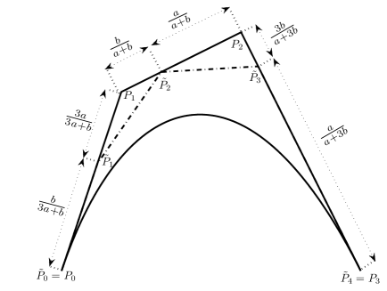
Figure 1: The dimension elevation process $\mathcal{E}_{(1)}(3)=span(1,t^{2},t^{3},t^{4})\subset\mathcal{E}_{\emptyset}(4)=span(1,t,t^{2},t^{3},t^{4})$. $(P_{0},P_{1},P_{2},P_{3})$ are the Chebyshev-Bézier points of a $\mathcal{E}_{(1)}(3)$-function, while $(\tilde{P}_{0},\tilde{P}_{1},\tilde{P}_{2},\tilde{P}_{3},\tilde{P}_{4})$ are the Chebyshev-Bézier points of the same function viewed as a $\mathcal{E}_{\emptyset}(4)$-function. (see example 11).

Theorem 8.

The Chebyshev-Bézier points $\tilde{P_{k}}$ in (78) are related to the Chebyshev-Bézier points $P_{k}$ by the relations

$$\tilde{P}_{0}=P_{0},\quad\tilde{P}_{n+1}=P_{n},$$

and for $k=1,2,...,n$

$$\tilde{P}_{k}=\rho_{[\lambda,\eta]}(n,k-1)\;P_{k-1}+\xi_{[\lambda,\eta]}(n,k)\;P_{k},$$ (79)

where $\xi_{[\lambda,\eta]}(n,k)$ and $\rho_{[\lambda,\eta]}(n,k)$ are given by

$$\xi_{[\lambda,\eta]}(n,k)=\frac{(n+1-k)a^{\lambda_{1}-\eta_{1}}}{n+1}{\binom{\eta}{\lambda}}_{\hskip-2.84544pt{n}}\Gamma_{\lambda}^{\eta}(n,k)$$

and

$$\rho_{[\lambda,\eta]}(n,k)=\frac{(k+1)b^{\lambda_{1}-\eta_{1}}}{n+1}{\binom{\eta}{\lambda}}_{\hskip-2.84544pt{n}}\Delta_{\lambda}^{\eta}(n,k),$$

where $\Gamma_{\lambda}^{\eta}(n,k)$ and $\Delta_{\lambda}^{\eta}(n,k)$ are defined in (67) and (68).

Remark 9.

As the relation (79) is independent of the $\mathcal{E}_{\lambda}(n)$-function $P$ and in view of (4), we have $\rho_{\lambda,\eta}(n,k-1)+\xi_{\lambda,\eta}(n,k)=1.$ This relation can also be directly proven (with rather great efforts) using Proposition 15.

Example 5.

Let $P$ be a $\mathcal{E}_{(1^{r})}(n)$-function. The partition $\eta=(0)$ is a dimension elevation partition of $\lambda$. Therefore, the function $P$ can be expressed as

$$P(t)=\sum_{k=0}^{n}B_{k,(1^{r})}^{n}(t)P_{k}=\sum_{k=0}^{n+1}B_{k}^{n+1}(t)\tilde{P}_{k}.$$

In this case, we have

$$\rho_{[1^{(r)},(0)]}(n,k-1)=\frac{kb}{r}\frac{e_{r-1}(a^{n-k+1},b^{k-1})}{e_{r}(a^{n-k+1},b^{k})}$$

and

$$\xi_{[1^{(r)},(0)]}(n,k)=\frac{(n+1-k)a}{r}\frac{e_{r-1}(a^{n-k},b^{k})}{e_{r}(a^{n-k+1},b^{k})}.$$

Therefore, from Theorem 8, we have $\tilde{P}_{0}=P_{0}$ and $\tilde{P}_{n+1}=P_{n}$ and for $k=1,...,n$,

$$\tilde{P}_{k}=\frac{kbe_{r-1}(a^{n-k+1},b^{k-1})}{re_{r}(a^{n-k+1},b^{k})}P_{k-1}+\frac{(n+1-k)ae_{r-1}(a^{n-k},b^{k})}{{re_{r}(a^{n-k+1},b^{k})}}P_{k}.$$

The case $r=1$ provide us with the following simple relationships

$$\tilde{P}_{k}=\frac{kb}{(n+1-k)a+kb}P_{k-1}+\frac{(n+1-k)a}{(n+1-k)a+kb}P_{k}.$$

Figure 1 shows an example of dimension elevation process for the case $r=1$.

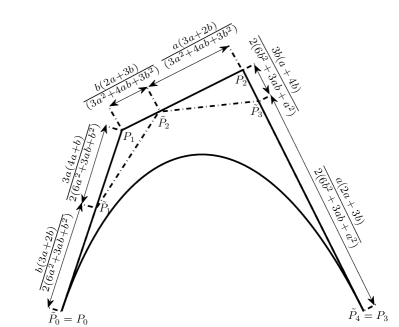
Figure 2: The dimension elevation process $\mathcal{E}_{(1,1)}(3)=span(1,t^{3},t^{4},t^{5})\subset\mathcal{E}_{(1)}(4)=span(1,t^{2},t^{3},t^{4},t^{5})$. $(P_{0},P_{1},P_{2},P_{3})$ are the Chebyshev-Bézier points of a $\mathcal{E}_{(1,1)}(3)$-function, while $(\tilde{P}_{0},\tilde{P}_{1},\tilde{P}_{2},\tilde{P}_{3},\tilde{P}_{4})$ are the Chebyshev-Bézier points of the same function viewed as a $\mathcal{E}_{(1)}(4)$-function. (see example 12).

Example 6.

Let us consider the dimension elevation process

$$\mathcal{E}_{(l)}(n)\subset\mathcal{E}_{(l-1)}(n+1).$$

Then, if we write

$$P(t)=\sum_{k=0}^{n}B_{k,(l)}^{n}(t)P_{k}=\sum_{k=0}^{n+1}B_{k,(l-1)}^{n+1}(t)\tilde{P}_{k},$$ (80)

we would have

$$\rho_{[(l),(l-1)]}(n,k-1)=\frac{kb}{l}\frac{h_{l-1}(a^{n-k+1},b^{k+1})}{h_{l}(a^{n-k+1},b^{k})}$$

and

$$\xi_{[(l),(l-1)]}(n,k)=\frac{(n+1-k)a}{l}\frac{h_{l-1}(a^{n+2-k},b^{k})}{h_{l}(a^{n-k+1},b^{k})}.$$

Therefore, we have $\tilde{P}_{0}=P_{0}$ and $\tilde{P}_{n+1}=P_{n}$ and for $k=1,...,n$,

$$\tilde{P}_{k}=\frac{kbh_{l-1}(a^{n-k+1},b^{k+1})}{lh_{l}(a^{n-k+1},b^{k})}P_{k-1}+\frac{(n+1-k)ah_{l-1}(a^{n+2-k},b^{k})}{{lh_{l}(a^{n-k+1},b^{k})}}P_{k}.$$

Figure 2 shows an example of the dimension elevation process for the case $l=2$.

8 Toward shaping with Young diagram

A polygon $\mathcal{P}=(P_{0},P_{1},...,P_{n})$ can be viewed as the control polygon of a $\mathcal{E}_{\lambda}(n)$-function, where $\lambda$ is a partition of length at most $n$. Therefore, by varying the partition $\lambda$, the curve associated with the control polygon will also vary accordingly. In such circumstances, the Young diagram can be viewed as a shape parameter. It would, therefore, be interesting to study the effect of standard operations on a fixed partition $\lambda$, such as adding a box, removing a box, adding a row or column and so on, on the shape of the curve. The problem is rather challenging and we will content ourself, here, with a simple experimental example. In Figure 3, we show the effect of adding boxes to the first row of the partition $\lambda=(2,1)$. Adding boxes to the first row seems to have the effect of making the curve more and more far from the control polygon. However, adding the same number of boxes to every column seems to have the opposite effect as shown in Figure 4.

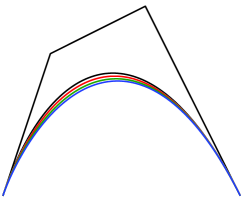
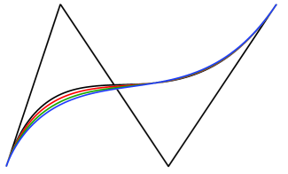
Figure 3: The effect of iteratively adding boxes to the first row of the partition $\lambda=(2,1)$. The black curve refers to the Chebyshev-Bézier curve over the interval $[a,b]=[1,4]$ associated with the partition $\lambda$, the red curve correspond to the partition $(3,1)$, the green curve to the partition $(4,1)$ and the blue curve to the partition $(5,1)$.

We can also define the tensor-product surfaces based on the Chebyshev-Bernstein basis associated with two different partitions. Namely, we can define a surface $\Gamma_{\lambda,\mu}$ by the parametric equation

$$\Gamma_{\lambda,\mu}(s,t)=\sum_{i,j=1}^{n}B_{i,\lambda}^{n}(t)B_{j,\mu}^{n}(s)P_{ij},$$ (81)

where $\lambda$ and $\mu$ are partitions of length at most $n$, $P_{ij}$ are points in $\mathbb{R}^{3}$ and $(s,t)\in[a,b]\times[c,d]$. Figure 5 shows an example of surfaces obtained from (81).

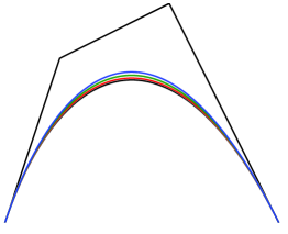
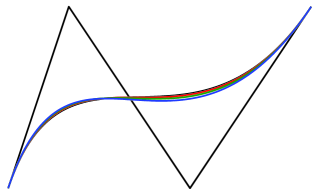
Figure 4: The effect of iteratively adding a column to the partition $\lambda=(2,1)$. The black curve refers to the Chebyshev-Bézier curve over the interval $[a,b]=[1,4]$ associated with the partition $\lambda$, the red curve correspond to the partition $(3,2,1)$, the green curve to the partition $(4,3,2)$ and the blue curve to the partition $(5,4,3)$.

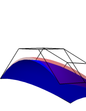
Figure 5: Tensor-product surfaces obtained using equation (81): the transparent surface is associated with the parameters $\lambda=(2,1)$, $\mu=(1,1)$ and $[a,b]=[c,d]=[3,4]$, while the blue surface is associated with the parameters $\lambda=(5,1)$, $\mu=(5,1)$ and $[a,b]=[c,d]=[1,6]$

.

8.1 Derivative the Chebyshev-Bernstein Basis

Consider a partition $\lambda=(\lambda_{1},\lambda_{2},...,\lambda_{n})$ of length at most $n$ in which we assume that

$$\lambda_{1}=\lambda_{2}.$$ (82)

Under the condition (82), the derivative of the Chebyshev-Bernstein element $B^{n}_{k,\lambda}$ is an element of the Chebyshev space $\mathcal{E}_{\lambda^{(0)}}(n-1)$ where $\lambda^{(0)}$ is the bottom partition of $\lambda$. Therefore, the derivative of $B^{n}_{k,\lambda}$ can be written as linear combination of the Chebyshev-Bernstein basis of $\mathcal{E}_{\lambda^{(0)}}(n-1)$. Using the vanishing property of the Chebyshev-Bernstein bases stated in Theorem 1, we derive as in (66) the following relationship

$$\frac{dB_{k,\lambda}^{n}(t)}{dt}=\frac{{B_{k,\lambda}^{n}}^{(k)}(a)}{{B_{k-1,\lambda^{(0)}}^{n-1}}^{(k-1)}(a)}B_{k-1,\lambda^{(0)}}^{n-1}(t)+\frac{{B_{k,\lambda}^{n}}^{(n-k)}(b)}{{B_{k,\lambda^{(0)}}^{n-1}}^{(n-k-1)}(b)}B_{k,\lambda^{(0)}}^{n-1}(t).$$ (83)

in which we adopt the convention that $B_{-1,\lambda^{(0)}}^{n-1}\equiv B_{n,\lambda^{(0)}}^{n-1}\equiv 0$. Let us denote by $\eta$ the partition $\eta=(\lambda_{3},...,\lambda_{n})$. The partition $\eta$ is the bottom partition of $\lambda^{(0)}$ and can well be written as $\eta=\left(\lambda^{(0)}\right)^{(0)}$, but for simplicity we will refer to this partition as $\eta$. Inserting in (83) the value of the derivatives from Theorem 6, we find

$$\frac{{B_{k,\lambda}^{n}}^{(k)}(a)}{{B_{k-1,\lambda^{(0)}}^{n-1}}^{(k-1)}(a)}=\frac{n}{b-a}\frac{f_{\lambda}(n+1)f_{\eta}(n-1)}{f_{\lambda^{(0)}}(n)^{2}}\frac{S_{\lambda^{(0)}}(a^{n-k},b^{k})S_{\lambda^{(0)}}(a^{n+1-k},b^{k-1})}{S_{\lambda}(a^{n+1-k},b^{k})S_{\eta}(a^{n-k},b^{k-1})}$$

and

$$\frac{{B_{k,\lambda}^{n}}^{(n-k)}(b)}{{B_{k,\lambda^{(0)}}^{n-1}}^{(n-k-1)}(b)}=-\frac{n}{b-a}\frac{f_{\lambda}(n+1)f_{\eta}(n-1)}{f_{\lambda^{(0)}}(n)^{2}}\frac{S_{\lambda^{(0)}}(a^{n-k},b^{k})S_{\lambda^{(0)}}(a^{n-1-k},b^{k+1})}{S_{\lambda}(a^{n-k},b^{k+1})S_{\eta}(a^{n-k-1},b^{k})}.$$

To write the formula for the derivative in a compact form, we define

Definition 7.

Let $\lambda=(\lambda_{1},\lambda_{2},...,\lambda_{n})$ be a partition of length $n\geq 2$. Let $a,b$ be real numbers. For $k=0,...,n$, we define the factor

$$R_{\lambda}(k,n)=\frac{S_{\lambda^{(0)}}(a^{n-k-1},b^{k+1})S_{\lambda^{(0)}}(a^{n-k},b^{k})}{S_{\lambda}(a^{n-k},b^{k+1})S_{\eta}(a^{n-k-1},b^{k})},$$ (84)

where $\lambda^{(0)}=(\lambda_{2},...,\lambda_{n}$ is the bottom partition of $\lambda$ and $\eta=(\lambda_{3},...,\lambda_{n}$ is the bottom partition of $\lambda^{(0)}$.

From the last definition and by noticing that

$$\frac{f_{\lambda}(n+1)f_{\eta}(n-1)}{f_{\lambda^{(0)}}(n)^{2}}=\frac{1}{\binom{\lambda}{\lambda^{(0)}}}_{n-1}$$

we obtain

Theorem 9.

Let $\lambda=(\lambda_{1},\lambda_{2},\lambda_{3},...,\lambda_{n})$ be a partition of length at most $n$ such that $\lambda_{1}=\lambda_{2}$. Then the derivative of the Chebyshev-Bernstein basis associated with the partition $\lambda$ over an interval $[a,b]$ satisfies

$$\frac{dB_{k,\lambda}^{n}(t)}{dt}=\frac{n}{(b-a)\binom{\lambda}{\lambda^{(0)}}}_{n-1}\left(R_{\lambda}(k-1,n)B_{k-1,\lambda^{(0)}}^{n-1}(t)-R_{\lambda}(k,n)B_{k,\lambda^{(0)}}^{n-1}(t)\right),$$

where $\lambda^{(0)}$ is the bottom partition of $\lambda$ and $R_{\lambda}(k,n)$ is defined in equation (84) and in which $\eta$ is the partition $\eta=(\lambda_{3},...,\lambda_{n})$. We adopt here the convention that $B_{-1,\lambda^{(0)}}^{n-1}\equiv B_{n,\lambda^{(0)}}^{n-1}\equiv 0$.

Note that in the case the partition $\lambda$ is the empty partition, we recover the classical formulas for the derivative of the polynomial Bernstein basis. Let $\lambda=(\lambda_{1},\lambda_{2},...,\lambda_{n})$ be a partition of length at most $n$ such that $\lambda_{1}=\lambda_{2}$ and Consider a $\mathcal{E}_{\lambda}(n)$-function $P$ written in the Chebyshev-Bernstein basis over an interval $[a,b]$ as

$$P(t)=\sum_{k=0}^{n}B_{k,\lambda}^{n}(t)P_{k}.$$

Using Theorem 6, we can express the derivative of the function $P$ in term of the Chebyshev-Bernstein basis over the interval $[a,b]$ of the space $\mathcal{E}_{\lambda^{(0)}}(n-1)$. Doing so leads to the following

Theorem 10.

Let $\lambda=(\lambda_{1},...,\lambda_{n})$ be a partition such that $\lambda_{1}=\lambda_{2}$ and let $P$ be a $\mathcal{E}_{\lambda}(n)$-function, written in the Chebyshev-Bernstein basis as

$$P(t)=\sum_{k=0}^{n}B_{k,\lambda}^{n}(t)P_{k}.$$

Then, we have

$$P^{\prime}(t)=\frac{n}{(b-a)\binom{\lambda}{\lambda^{(0)}}}_{n-1}\sum_{k=0}^{n-1}R_{\lambda}(k,n)B_{k,\lambda^{(0)}}^{n-1}(t)\Delta P_{k},$$

where $\Delta P_{i}=P_{i+1}-P_{i}$ and $R_{\lambda}(k,n)$ is given in (84).

In particular, we have

$$\begin{split}P^{\prime}(a)&=\frac{na^{\lambda_{1}}}{b-a}\frac{f_{\lambda}(n+1)}{f_{\lambda^{(0)}}(n)}\frac{S_{\lambda^{(0)}}(a^{n-1},b)}{S_{\lambda}(a^{n},b)}\left(P_{1}-P_{0}\right),\\ P^{\prime}(b)&=\frac{nb^{\lambda_{1}}}{b-a}\frac{f_{\lambda}(n+1)}{f_{\lambda^{(0)}}(n)}\frac{S_{\lambda^{(0)}}(a,b^{n-1})}{S_{\lambda}(a,b^{n})}\left(P_{n}-P_{n-1}\right).\end{split}$$ (85)

As from Theorem 6, we know the derivatives $(B_{1,\lambda}^{n})^{\prime}(a)$ and $(B_{n-1,\lambda}^{n})^{\prime}(b)$ and by using the fact that the segments $[P_{0},P_{1}]$ and $[P_{n-1},P_{n}]$ are tangents to the curve at the point $P(a)$ and $P(b)$ respectively, we can show that the equations (85) are true independently if the partition $\lambda$ has it first two parts equals or not. It is rather interesting that computing the derivative $(B_{0,\lambda}^{n})^{\prime}(a)$ or $(B_{n,\lambda}^{n})^{\prime}(a)$ using the explicit expression of the Chebyshev-Bernstein basis (48) reveal to be difficult. Equations (85) can be used to achieve the $C^{1}$ continuity between two Chebyshev-Bézier curves associated with two different partitions, as follows

Corollary 6.

Let $\lambda=(\lambda_{1},\lambda_{2},...,\lambda_{n}$ and $\mu=(\mu_{1},\mu_{2},...,\mu_{n})$ be two partitions of length at most $n$ and let $\mathcal{P}=(P_{0},P_{1},...,P_{n})$ (resp. $(\mathcal{Q}=Q_{0},Q_{1},...,Q_{n})$) be the Chebyshev-Bézier points of a $\mathcal{E}_{\lambda}(n)$ (resp. a $\mathcal{E}_{\mu}(n)$) function over an interval $[a,b]$ (resp. $[b,c]$). Then the composite curve $\gamma$ formed by the two curves associated with the two control polygons $\mathcal{P}$ and $\mathcal{Q}$ is $C^{1}$ at $b$ if and only if $P_{n}=Q_{0}$ and

$$\frac{nb^{\lambda_{1}}}{b-a}\frac{f_{\lambda}(n+1)}{f_{\lambda^{(0)}}(n)}\frac{S_{\lambda^{(0)}}(a,b^{n-1})}{S_{\lambda}(a,b^{n})}\left(P_{n}-P_{n-1}\right)=\frac{nb^{\mu_{1}}}{c-b}\frac{f_{\mu}(n+1)}{f_{\mu^{(0)}}(n)}\frac{S_{\mu^{(0)}}(c,b^{n-1})}{S_{\mu}(c,b^{n})}\left(Q_{1}-Q_{0}\right).$$

Example 7.

Consider the Chebyshev-Bézier curve $\Gamma_{1}$ of order $n$ associated with the partition $\lambda=(1^{k})$ with $k\leq n$ and control polygon $(P_{0},P_{1},....,P_{n})$ over an interval $[a,b]$. Consider another Chebyshev-Bézier curve $\Gamma_{2}$ of order $n$ associated with the empty partition and control polygon $(Q_{0},Q_{1},....Q_{n})$ over an interval $[b,c]$. From equations (85), a necessary and sufficient condition for the two curves $\Gamma_{1}$ and $\Gamma_{2}$ to be $C^{1}$ at the point $P_{n}$ is that

$$P_{n}=Q_{0}\quad\textnormal{and}\quad\frac{n(n+1)b}{k(b-a)}\frac{e_{k-1}(a,b^{n-1})}{e_{k}(a,b^{n})}(P_{n}-P_{n-1})=\frac{n}{c-b}(Q_{1}-Q_{0}).$$

If we denote by $\rho$ the positive number such that $P_{n}-P_{n-1}=\rho(Q_{1}-Q_{0})$, then, from the last equation, in order to achieve the $C^{1}$ continuity at $P_{n}$, we should choose the number $c$ as

$$c=b+\frac{k(b-a)e_{k}(a,b^{n})}{(n+1)b\rho e_{k-1}(a,b^{n-1})}.$$ (86)

Figure 6 shows the case $n=3$ in this example, while Figure 7 shows another example of the application of Corollary 6 with the partitions $\lambda=(2,1)$ and $\mu=(1,1)$.

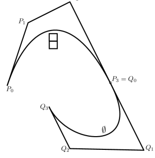
Figure 6: $C^{1}$ continuity at the point $P_{3}$ between two Chebyshev-Bézier curves associated with two differents partitions. The Chebyshev-Bézier curve with Chebyshev-Bézier points $(P_{0},P_{1},P_{2},P_{3})$ is associated to the partition $(1,1)$ and parametrized over the interval $[a,b]=[1,3]$. The Chebyshev-Bézier curve with Chebyshev-Bézier points $(Q_{0},Q_{1},Q_{2},Q_{3})$ is associated to the empty partition and parametrized over the interval $[3,c]$, where the parameter $c$ was computed using equation (86) to achieve the $C^{1}$ continuity. (see example 13)

Remark 10.

If a partition $\lambda=(\lambda_{1},\lambda_{2},...,\lambda_{n})$ of length at most $n$ satisfies $\lambda_{1}=\lambda_{2}=...=\lambda_{s},$ $s\leq n$, then we can iterate Theorem 9 to compute the derivatives up to order $s-1$ of the Chebyshev-Bernstein basis.

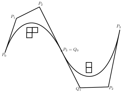
Figure 7: $C^{1}$ continuity at the point $P_{3}$ between two Chebyshev-Bézier curves associated with two differents partitions. The Chebyshev-Bézier curve with Chebyshev-Bézier points $(P_{0},P_{1},P_{2},P_{3})$ is associated to the partition $(2,1)$ and parametrized over the interval $[a,b]=[1,3]$. The Chebyshev-Bézier curve with Chebyshev-Bézier points $(Q_{0},Q_{1},Q_{2},Q_{3})$ is associated to the partition $(1,1)$ and parametrized over the interval $[3,c]$, where the parameter $c$ was computed using the conditions of corollary 6 to achieve the $C^{1}$ continuity.

Consider, now, a partition $\lambda=(\lambda_{1},\lambda_{2},...,\lambda_{n})$ of length at most $n$ in which we assume this time that $\lambda_{1}\neq\lambda_{2}$. Under this condition, the derivative of the Chebyshev-Bernstein element $B^{n}_{k,\lambda}$ over an interval $[a,b]$ is an element of the Chebyshev space $\mathcal{E}_{\mu}(n)$ where $\mu$ is the partition $\mu=(\lambda_{1}-1,\lambda_{2},...,\lambda_{n})$. The derivative of $B^{n}_{k,\lambda}$ can be written as linear combination of the Chebyshev-Bernstein basis of $\mathcal{E}_{\mu}(n)$. However, if we use the vanishing properties of the Chebyshev-Bernstein bases, we arrive to a three-term recurrence relation between the two Chebyshev-Bernstein bases and in which Theorem 6 does not allow for an easy way to compute the necessary coefficients. To solve this problem, we can instead proceed as follows : As $\lambda_{1}\neq\lambda_{2}$, we have necessarily $\lambda_{1}>\lambda_{2}$. Therefore, the partition $\eta=(\lambda_{1}-1,\lambda_{1}-1,\lambda_{2},...,\lambda_{n})$ is a dimension elevation partition of $\lambda$. We can compute the Chebyshev-Bernstein basis of $\mathcal{E}_{\eta}(n+1)$ as a function of the Chebyshev-Bernstein basis of $\mathcal{E}_{\lambda}(n)$ according to Theorem 7. Now the partition $\eta$ satisfy the condition that its first two parts are equals, and therefore, we can use Theorem 9 to compute the derivative. Proceeding along these two steps, in which we omit the computation as they can be readily done, we find

Theorem 11.

Let $\lambda=(\lambda_{1},\lambda_{2},\lambda_{3},...,\lambda_{n})$ be a partition of length at most $n$ such that $\lambda_{1}\neq\lambda_{2}$. Then the derivative of the Chebyshev-Bernstein basis associated with the partition $\lambda$ over an interval $[a,b]$ satisfies

$$\frac{dB_{k,\lambda}^{n}(t)}{dt}=\frac{\binom{\eta}{\lambda}_{n}}{(b-a)\binom{\eta}{\mu}_{n}}\left(G_{1}(k,n)B_{k-1,\mu}^{n}(t)+G_{2}(k,n)B_{k,\mu}^{n}(t)+G_{3}(k,n)B_{k+1,\mu}^{n}(t)\right),$$

where

$$G_{1}(k,n)=(n+1-k)a\Gamma_{\lambda}^{\eta}(n,k)R_{\eta}(k-1,n+1),$$

$$G_{2}(k,n)=R_{\eta}(k,n+1)\big{(}(k+1)b\Delta_{\lambda}^{\eta}(n,k)-(n+1-k)a\Gamma_{\lambda}^{\eta}(n,k)\big{)},$$

and

$$G_{3}(k,n)=-(k+1)b\Delta_{\lambda}^{\eta}(n,k)R_{\eta}(k+1,n+1).$$

and the partition $\eta$ and $\mu$ are given by $\eta=(\lambda_{1}-1,\lambda_{1}-1,\lambda_{2},...,\lambda_{n})$ and $\mu=(\lambda_{1}-1,\lambda_{2},...,\lambda_{n})$, the factors $\Delta_{\lambda}^{\eta}$, $\Gamma_{\lambda}^{\eta}(n,k)$ and $R_{\eta}$ are defined in (67), (68) and (84) respectively. We adopt the convention that $B_{-1,\mu}^{n}\equiv B_{n+1,\mu}^{n}\equiv 0$.

Let $\lambda=(\lambda_{1},\lambda_{2},...,\lambda_{n})$ be a partition of length at most $n$ such that $\lambda_{1}\neq\lambda_{2}$ and consider a $\mathcal{E}_{\lambda}(n)$-function $P$ written in the Chebyshev-Bernstein basis over an interval $[a,b]$ as

$$P(t)=\sum_{k=0}^{n}B_{k,\lambda}^{n}(t)P_{k}.$$

Using Theorem 11, we can express the derivative of the function $P$ in term of the Chebyshev-Bernstein basis over the interval $[a,b]$ of the space $\mathcal{E}_{\mu}(n)$. Doing so leads to the following

Theorem 12.

Let $\lambda=(\lambda_{1},...,\lambda_{n})$ be a partition such that $\lambda_{1}\neq\lambda_{2}$ and let $P$ be a $\mathcal{E}_{\lambda}(n)$-function, written in the Chebyshev-Bernstein basis over an interval $[a,b]$ as

$$P(t)=\sum_{k=0}^{n}B_{k,\lambda}^{n}(t)P_{k}.$$

Then, we have

$$P^{\prime}(t)=\frac{\binom{\eta}{\lambda}_{n}}{(b-a)\binom{\eta}{\mu}_{n}}\sum_{k=0}^{n}\left(G_{3}(k-1,n)P_{k-1}+G_{2}(k,n)P_{k}+G_{1}(k+1,n)P_{k+1}\right),B_{k,\mu}^{n}(t)$$

where the factors $G_{1},G_{2},G_{3}$ and the partitions $\eta$ and $\mu$ are defined in Theorem 11.

9 Conclusions

In this paper, we carried out a comprehensive study of the notion of Chebyshev blossom in Müntz spaces, thereby showing their adequacy in free-form design schemes. An interesting aspect of the work was the followed methodology in providing for an explicit expression of the Chebyshev-Bernstein basis. Most of the steps in the proof were combinatorial in nature. Similar arguments, therefore, could be applied to any extended Chebyshev space constructed from weight functions, in the sense that the condensation formula will provide us with the pseudo-affinity factor and in which the combinatorics of the de Casteljau paths can be employed to give extra-information on the derivatives of the Chebyshev-Bernstein basis. Such a program will be the object of a forthcoming contribution. Moreover, the problem of higher order continuity and the issue of shaping with Young diagrams lead to interesting problems for future work.

Acknowledgement : This work was partially supported by the MEXT Global COE project.

References

[1] R. Ait-Haddou, T. Nomura and L. Biard, A refinement of the variation
diminishing property of Bézier curves, Comput. Aided Geom. Design, Volume 27, Issue 2, 202–211, 2010
[2] J.M. Aldaz, O. Kounchev, H. Render, Shape preserving properties of
Bernstein operators on extended Chebyshev spaces, Numer. Math. 114 (1) (2009) 1 25.
[3]D. Bowman and D.M. Bradley, The Algebra and Combinatorics of Shuffles and Multiple Zeta Values
J. Combin. Theory Ser. A , Vol 97, Issue 1,(2002),43-61