Turbulent Oxygen Flames in Type Ia Supernovae

Abstract

In previous studies, we examined turbulence-flame interactions in carbon-burning thermonuclear flames in Type Ia supernovae. In this study, we consider turbulence-flame interactions in the trailing oxygen flames. The two aims of the paper are to examine the response of the inductive oxygen flame to intense levels of turbulence, and to explore the possibility of transition to detonation in the oxygen flame. Scaling arguments analogous to the carbon flames are presented and then compared against three-dimensional simulations for a range of Damköhler numbers ($\mathrm{Da}_{16}$) at a fixed Karlovitz number. The simulations suggest that turbulence does not significantly affect the oxygen flame when $\mathrm{Da}_{16}<1$, and the flame burns inductively some distance behind the carbon flame. However, for $\mathrm{Da}_{16}>1$, turbulence enhances heat transfer and drives the propagation of a flame that is narrower than the corresponding inductive flame would be. Furthermore, burning under these conditions appears to occur as part of a combined carbon-oxygen turbulent flame with complex compound structure. The simulations do not appear to support the possibility of a transition to detonation in the oxygen flame, but do not preclude it either.

1 INTRODUCTION

A major uncertainty in the modeling of Type Ia supernovae (SN Ia) is the physical process whereby a subsonic deflagration transitions to a detonation. Such a transition seems to be required by the observations (Kozma et al., 2005; Hoflich et al., 1995; Mazzali et al., 2007; Kasen et al., 2009), at least within the context of the popular “single degenerate” Chandrasekhar-mass model. Previous papers (e.g. Khokhlov et al., 1997; Niemeyer & Woosley, 1997; Woosley et al., 2009; Aspden et al., 2010) have focused on the possibility of a transition to detonation in carbon-rich material as the deflagration enters the “distributed burning regime” where burning becomes slow enough for turbulence to disrupt the flame, mixing hot ash and cold fuel. Other papers (e.g. Plewa et al., 2004) have explored the possibility that detonation may be mechanically induced by the collision of burning waves near the surface of the white dwarf. The present situation is inconclusive. The collisions may not be strong enough to robustly cause a detonation (Röpke et al., 2007) and the amount of turbulence required for a spontaneous detonation in the distributed regime is quite large (Woosley et al., 2009).

Here we consider a third possibility - that the necessary carbon detonation actually begins as an oxygen detonation in a hybrid flame. This possibility has been recently considered (Woosley et al., 2010) in a one-dimensional study. Carbon burning produces oxygen-rich ash that still contains a large potential reservoir of nuclear energy. The oxygen ash is produced, for a given fuel density, at a constant temperature that gradually rises as a result of oxygen burning, until, finally, a silicon-rich composition is produced. As a result of turbulence, this oxygen layer, which we shall refer to as an oxygen “flame”, is broadened and islands of nearly isothermal conditions are produced. Here we flesh out those one-dimensional results in a series of three-dimensional simulations.

In two previous three-dimensional studies, Aspden et al. (2008a, 2010) (henceforth Papers I and II), turbulence-flame interactions in carbon-burning flames were examined at small and large scales, respectively. In Paper I, it was shown that once the turbulence was sufficiently strong, the mixing of fuel and heat was driven by turbulent mixing instead of thermal diffusion. This resulted in a categorically different kind of flame, which was referred to as a distributed flame. Paper II extended these small-scale studies to (more realistic) larger length scales, where scaling relations based on the theory of Damköhler (1940) were predicted to reach a limiting behavior, resulting in a so-called “$\lambda$-flame”.

In this paper, we focus on turbulence-flame interactions in the trailing oxygen flame, which are expected to be significantly different than in the carbon flame, due to the inductive nature of the oxygen burning. The specific question we address is whether turbulence can lead to a greatly extended oxygen-rich region that might have properties suitable for detonation.

2 THEORETICAL DESCRIPTION

We first recap the scaling relations for turbulent carbon flames from Paper II, and then present theory describing possible modes of burning in turbulent oxygen flames. We fix the fuel to be carbon-oxygen at a particular density and temperature, and then choose turbulent conditions based on the flame properties of the fuel. Since the oxygen burning time scale is determined by the temperature resulting from carbon burning at the given density, the width of the oxygen flame is most sensitive to that density and the turbulence properties. For typical turbulent conditions in the supernova and an initial composition of 40% carbon and 60% oxygen, Woosley et al. (2010) find that the density of greatest interest is $\rho_{12}=2.5\times 10^{7}$ g cm^-3 (we use $\rho$ and $T$ for total density and temperature the suffix 12 denotes conditions before the carbon burns). This gives a post-carbon-flame temperature and density of approximately $T_{16}=3.14\times 10^{9}$ K and $\rho_{16}=1.69\times 10^{7}$ g/cm³, respectively (here suffix 16 denotes conditions after carbon burning but before oxygen has burned). Under these conditions, the oxygen flame has an inductive burning time scale of approximately $\tau_{16}=0.016$ s, see Woosley et al. (2010).

Having fixed the fuel conditions, the two parameters that can be varied are the rms turbulent velocity fluctuation $\check{u}$ and the integral length scale $l$. Turbulent premixed flames are characterized through Karlovitz and Damköhler numbers

$$\mathrm{Ka}^{2}_{L}=\frac{\check{u}^{3}l_{L}}{s_{L}^{3}l},\quad\quad\mathrm{and}\quad\quad\mathrm{Da}_{L}=\frac{s_{L}l}{\check{u}l_{L}},$$ (1)

where $s_{L}$ and $l_{L}$ are the laminar flame speed and width, respectively. These quantities represent the ratio of turbulent time scales at the Kolmogorov and integral length scales, respectively, and are two dimensionless quantities that represent the parameter space. As in Paper II, we focus on a fixed $\mathrm{Ka}_{L}$, corresponding to fixing the energy dissipation rate $\varepsilon^{*}=\check{u}^{3}/l$ of the turbulence in the star. For fixed $\mathrm{Ka}_{L}$ and $\varepsilon^{*}$, $\check{u}=(\varepsilon^{*}l)^{1/3}$, it can be shown that $\mathrm{Da}_{L}\propto l^{2/3}$. Therefore, the parameter space is one-dimensional and can be represented equivalently by either $\mathrm{Da}_{L}$ or $l$.

We assume that the Karlovitz number is constant and sufficiently high to obtain a distributed carbon flame, see Paper I. The turbulent carbon flame properties will then depend on its turbulent nuclear burning time scale $\tau_{12}^{T}$ (note the superscript $T$ differentiates the turbulent from laminar burning time scales, again see Paper I), and the properties of the turbulence, specifically the integral length scale $l$ (recall that the turbulent intensity at fixed Karlovitz number is determined by $\check{u}=(\varepsilon^{*}l)^{1/3}$). Following Paper II and Damköhler (1940), by analogy with laminar flames, the turbulent flame speed $s_{12}^{T}$ and width $l_{12}^{T}$ can be expressed in terms of $\tau_{12}^{T}$ and a turbulent diffusion coefficient $\mathcal{D}_{T}$ (not to be confused with the Damköhler number $\mathrm{Da}$) as

$$s_{12}^{T}=\sqrt{\frac{\mathcal{D}_{T}}{\tau_{12}^{T}}},\quad\quad\mathrm{and}\quad\quad l_{12}^{T}=\sqrt{\mathcal{D}_{T}\tau_{12}^{T}},$$ (2)

respectively. These relations only hold when the time scale of the turbulent eddies is shorter than the turbulent nuclear time scale of the carbon fuel, i.e. for $\mathrm{Da}_{12}^{T}=\tau/\tau_{12}^{T}\lower 0.43057pt\hbox{\hbox to0.0pt{\raise 2.58334pt\hbox{\hskip 1.29167pt{{$\scriptscriptstyle<$}}}\hss} \kern-1.72218pt{{$\scriptscriptstyle\sim$}}}1$, where $\tau$ is the turbulence time scale $\tau=l/\check{u}$. Taking a simple approximation $\mathcal{D}_{T}=\check{u}l$, the turbulent flame speed and width were both shown to be proportional to $\mathrm{Da}_{12}^{T}$ when $\mathrm{Da}_{12}^{T}\lower 0.43057pt\hbox{\hbox to0.0pt{\raise 2.58334pt\hbox{\hskip 1.29167pt{{$\scriptscriptstyle<$}}}\hss} \kern-1.72218pt{{$\scriptscriptstyle\sim$}}}1$. For $\mathrm{Da}_{12}^{T}\lower 0.43057pt\hbox{\hbox to0.0pt{\raise 2.58334pt\hbox{\hskip 1.29167pt{{$\scriptscriptstyle>$}}}\hss} \kern-1.72218pt{{$\scriptscriptstyle\sim$}}}1$, the turbulence can no longer broaden the flame, and the limiting $\lambda$-flame behavior is reached (see Paper II), with local turbulent speed $s_{12}^{\lambda}$ and width $\lambda_{12}$ that depend on $\varepsilon^{*}$ and $\tau_{12}^{T}$ only, according to the relations

$$s_{12}^{\lambda}=\sqrt{\varepsilon^{*}\tau_{12}^{T}}\quad\quad\mathrm{and}\quad\quad\lambda_{12}=\sqrt{\varepsilon^{*}{\tau_{12}^{T}}^{3}},$$ (3)

respectively. Note that $s_{12}^{\lambda}$ and $\lambda_{12}$ are both constant. The turbulent flame speed and width can therefore be written as

$$\frac{s_{12}^{T}}{s_{12}^{\lambda}}=\frac{l_{16}^{T}}{\lambda_{12}}=\left\{\begin{array}[]{ll}\mathrm{Da}_{12}^{T}&\mathrm{for\ }\mathrm{Da}_{12}^{T}\lower 0.43057pt\hbox{\hbox to0.0pt{\raise 2.58334pt\hbox{\hskip 1.29167pt{{$\scriptscriptstyle<$}}}\hss} \kern-1.72218pt{{$\scriptscriptstyle\sim$}}}1,\\ 1&\mathrm{otherwise}.\end{array}\right.$$ (4)

We now apply this theoretical approach to oxygen flames, where there are three potential modes of burning: inductive, turbulent or $\lambda$-flame. Each mode will have a corresponding local flame width and speed, which will be denoted $(l_{16},s_{16})$, $(l_{16}^{T},s_{16}^{T})$, and $(l_{16}^{\lambda},s_{16}^{\lambda})$, respectively.

The inductive mode is the simplest and is considered first. In a frame of reference where the carbon flame is stationary, the incoming fluid speed is equal to the flame speed $u_{0}=s_{12}$. The resulting oxygen flame has a width equal to $l_{16}=u_{0}\tau_{16}$, where the time taken for the oxygen to burn at a given density and temperature is $\tau_{16}$. In the presence of turbulence, the carbon flame speed is enhanced, but the oxygen flame remains slaved to carbon flame, and $l_{16}=u_{0}\tau_{16}$, only with $u_{0}=s_{12}^{T}$. In the large-scale turbulence limit (see Damköhler (1940); Peters (1999, 2000)), the turbulent carbon flame speed will be close to the turbulent intensity, and so we can take $u_{0}=\beta\check{u}$, where $\beta$ should be expected to be order unity, but can be as high as three, accounting for fluctuations and the density jump across the carbon flame. This defines $s_{16}=\beta\check{u}$ and $l_{16}=\beta\check{u}\tau_{16}$ for a turbulent oxygen flame burning inductively.

Defining Karlovitz and Damköhler numbers for oxygen flames

$$\mathrm{Ka}^{2}_{16}=\frac{\check{u}^{3}l_{16}}{s_{16}^{3}l},\quad\quad\mathrm{and}\quad\quad\mathrm{Da}_{16}=\frac{s_{16}l}{\check{u}l_{16}},$$ (5)

reveals an interesting difference from carbon flames. Using $s_{16}=\beta\check{u}$, it can be shown that $\beta^{2}\mathrm{Ka}_{16}^{2}\mathrm{Da}_{16}\equiv 1$, which means that the parameter space for oxygen flames is one-dimensional. Therefore, under the assumption that the carbon flame is in the large-scale turbulence limit (so $s_{16}=\beta\check{u}$), the behavior of oxygen flames can be classified through the Damköhler number $\mathrm{Da}_{16}$ alone. Note that for a fixed fuel, all of the relevant Damköhler numbers are constant multiples of each other, e.g. $\mathrm{Da}_{16}=\sigma\mathrm{Da}_{12}^{T}$, where $\sigma=\tau_{12}^{T}/\tau_{16}$ is a constant. Also note that both $s_{16}$ and $l_{16}$ can be shown to be proportional to $\mathrm{Da}_{16}^{1/2}$.

If turbulent mixing can drive the flame, similar to the behavior in Paper II, scaling relations for turbulent flame speed and width can be predicted in terms of the oxygen burning time scale and the turbulent diffusion coefficient $\mathcal{D}_{T}$ as $s_{16}^{T}=\sqrt{\mathcal{D}_{T}/\tau_{16}}$ and $l_{16}^{T}=\sqrt{\mathcal{D}_{T}\tau_{16}}$. These scaling relations should only be expected to be possible for low values of the oxygen Damköhler number, i.e. $\mathrm{Da}_{16}=\lower 0.43057pt\hbox{\hbox to0.0pt{\raise 2.58334pt\hbox{\hskip 1.29167pt{{$\scriptscriptstyle<$}}}\hss} \kern-1.72218pt{{$\scriptscriptstyle\sim$}}}1$. On the other hand, for $\mathrm{Da}_{16}\lower 0.43057pt\hbox{\hbox to0.0pt{\raise 2.58334pt\hbox{\hskip 1.29167pt{{$\scriptscriptstyle>$}}}\hss} \kern-1.72218pt{{$\scriptscriptstyle\sim$}}}1$, it may be possible to produce an oxygen $\lambda$-flame, where the flame speed and width would be $s_{16}^{\lambda}=\sqrt{\varepsilon^{*}\tau_{16}}$ and $\lambda_{16}=\sqrt{\varepsilon^{*}{\tau_{16}}^{3}}$, respectively. As above, the turbulent oxygen flame speed and width can be predicted to be

$$\frac{s_{16}^{T}}{s_{16}^{\lambda}}=\frac{l_{16}^{T}}{\lambda_{16}}=\left\{\begin{array}[]{ll}\mathrm{Da}_{16}&\mathrm{for\ }\mathrm{Da}_{16}\lower 0.43057pt\hbox{\hbox to0.0pt{\raise 2.58334pt\hbox{\hskip 1.29167pt{{$\scriptscriptstyle<$}}}\hss} \kern-1.72218pt{{$\scriptscriptstyle\sim$}}}1,\\ 1&\mathrm{otherwise}.\end{array}\right.$$ (6)

The simulations in this study correspond to full-star conditions where $\check{u}^{*}=2\times 10^{7}$ cm/s on an integral length scale of $L^{*}=1\times 10^{6}$ cm, giving an energy dissipation rate of $\varepsilon^{*}=8\times 10^{15}$ cm²/s³, (see Röpke, 2007). Carbon fuel (40%) at $\rho_{12}=2.5\times 10^{7}$ g/cm³ and $T_{12}=6\times 10^{8}$ K burns to $\rho_{16}=1.69\times 10^{7}$ g/cm³ and $T_{16}=3.14\times 10^{9}$ K, which has an inductive time scale for oxygen of $0.016$ s. This gives an oxygen $\lambda$-flame speed and width of $s_{16}^{\lambda}=1.13\times 10^{7}$ cm/s, and $\lambda_{16}=1.81\times 10^{5}$ cm, respectively.

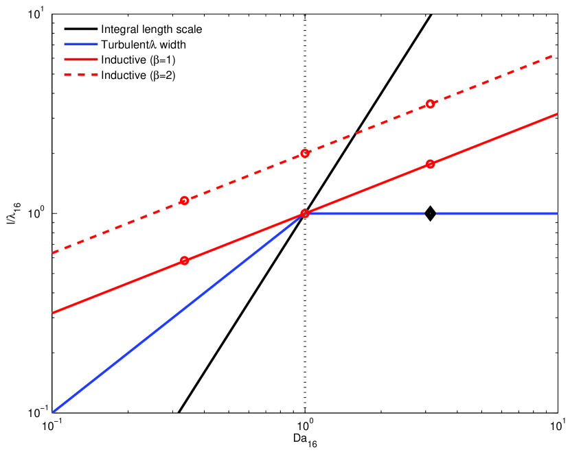
Figure 1: Scaling relations for oxygen flame widths as a function of $\mathrm{Da}_{16}$. The red lines show the inductive flame width $l_{16}$ (solid for $\beta=1$, and dashed for $\beta=2$). The blue line shows the turbulent width $l_{16}^{T}$ if turbulent mixing drives the flame, which scales with $\mathrm{Da}_{16}$ for $\mathrm{Da}_{16}\lower 0.43057pt\hbox{\hbox to0.0pt{\raise 2.58334pt\hbox{\hskip 1.29167pt{{$\scriptscriptstyle<$}}}\hss} \kern-1.72218pt{{$\scriptscriptstyle\sim$}}}1$ and is equal to the $\lambda$-flame thickness for $\mathrm{Da}_{16}\lower 0.43057pt\hbox{\hbox to0.0pt{\raise 2.58334pt\hbox{\hskip 1.29167pt{{$\scriptscriptstyle>$}}}\hss} \kern-1.72218pt{{$\scriptscriptstyle\sim$}}}1$ .

Figure 1 depicts the scaling relations for the different turbulent flame widths as a function of Damköhler number. Recall $\mathrm{Da}_{16}\propto l^{2/3}$, so this can be thought of as a function of integral length scale, shown by the thick black line. The red lines show the normalized inductive flame width $l_{16}/\lambda_{16}$ (solid for $\beta=1$, and dashed for $\beta=2$). The blue line shows the normalized turbulent width $l_{16}^{T}/\lambda_{16}=\mathrm{Da}_{16}$ for ($\mathrm{Da}_{16}\lower 0.43057pt\hbox{\hbox to0.0pt{\raise 2.58334pt\hbox{\hskip 1.29167pt{{$\scriptscriptstyle<$}}}\hss} \kern-1.72218pt{{$\scriptscriptstyle\sim$}}}1$) and $l_{16}^{T}/\lambda_{16}=1$ for ($\mathrm{Da}_{16}\lower 0.43057pt\hbox{\hbox to0.0pt{\raise 2.58334pt\hbox{\hskip 1.29167pt{{$\scriptscriptstyle>$}}}\hss} \kern-1.72218pt{{$\scriptscriptstyle\sim$}}}1$), if turbulent mixing drives the flame. The red circles correspond to the simulations that will be considered in this study, specifically $\mathrm{Da}_{16}=1/3$, $1$, and $3$, with $\beta=1$ and $2$, and will be described in detail below.

The black diamond highlights the $\lambda$-flame thickness at $\mathrm{Da}_{16}=3$, which is smaller than the corresponding inductive flame widths. This means that the possibility of an oxygen $\lambda$-flame is particularly interesting as it would be an example of turbulence giving rise to a flame that is narrower than its zero turbulence counterpart. This is counterintuitive, as one expects turbulence to broaden interfaces. However, in this case, turbulence acts to enhance heat transfer, allowing the flame to burn more rapidly; turbulence can mix hot ash with cold fuel more rapidly than the fuel is heated through inductive burning.

3 SIMULATION DESCRIPTION

As in Papers I and II, we use a low Mach number hydrodynamics code, adapted to the study of thermonuclear flames, as described in Bell et al. (2004). The advantage of this method is that sound waves are filtered out analytically, so the time step is set by the bulk fluid velocity and not the sound speed. This is an enormous efficiency gain for low speed flames. We note that in all simulations presented here, the Mach number remains below 0.1 (usually by an order of magnitude), and so compressibility effects are considered to be negligible. The reactions rate here are taken from Caughlan & Fowler (1988) with screening. The conductivities are those reported in Timmes (2000), and the equation of state is the Helmholtz free-energy based general stellar EOS described in Timmes & Swesty (2000). We note that we do not utilize the Coulomb corrections to the electron gas in the general EOS, as these are expected to be minor at the conditions considered.

The non-oscillatory finite-volume scheme employed here permits the use of implicit large eddy simulation (iles). This technique captures the inviscid cascade of kinetic energy through the inertial range, while the numerical error acts in a way that emulates the dissipative physical effects on the dynamics at the grid scale, without the expense of resolving the entire dissipation subrange. An overview of the technique can be found in Grinstein et al. (2007). Aspden et al. (2008b) presented a detailed study of the technique using the present numerical scheme, including a characterization that allowed for an effective viscosity to be derived. Thermal diffusion plays a significant role in the flame dynamics, so it is explicitly included in the model. Species diffusion is significantly smaller, so it is not included explicitly, but will be subject to numerical diffusion, which can be considered to have an effective unity Schmidt number and exhibit the same behavior observed for viscosity in Aspden et al. (2008b).

The turbulent velocity field was maintained using the forcing term used in Papers I, II and Aspden et al. (2008b). Specifically, a forcing term was included in the momentum equations consisting of a superposition of long wavelength Fourier modes with random amplitudes and phases. The forcing term is scaled by density so that the forcing is somewhat reduced in the ash. This approach provides a way to embed the flame in a turbulent background, mimicking the much larger inertial range that these flames would experience in a type Ia supernova, without the need to resolve the large-scale convective motions that drive the turbulent energy cascade. Aspden et al. (2008b) demonstrated that the effective Kolmogorov length scale is approximately $0.28\Delta x$, and the integral length scale is approximately a tenth of the domain width.

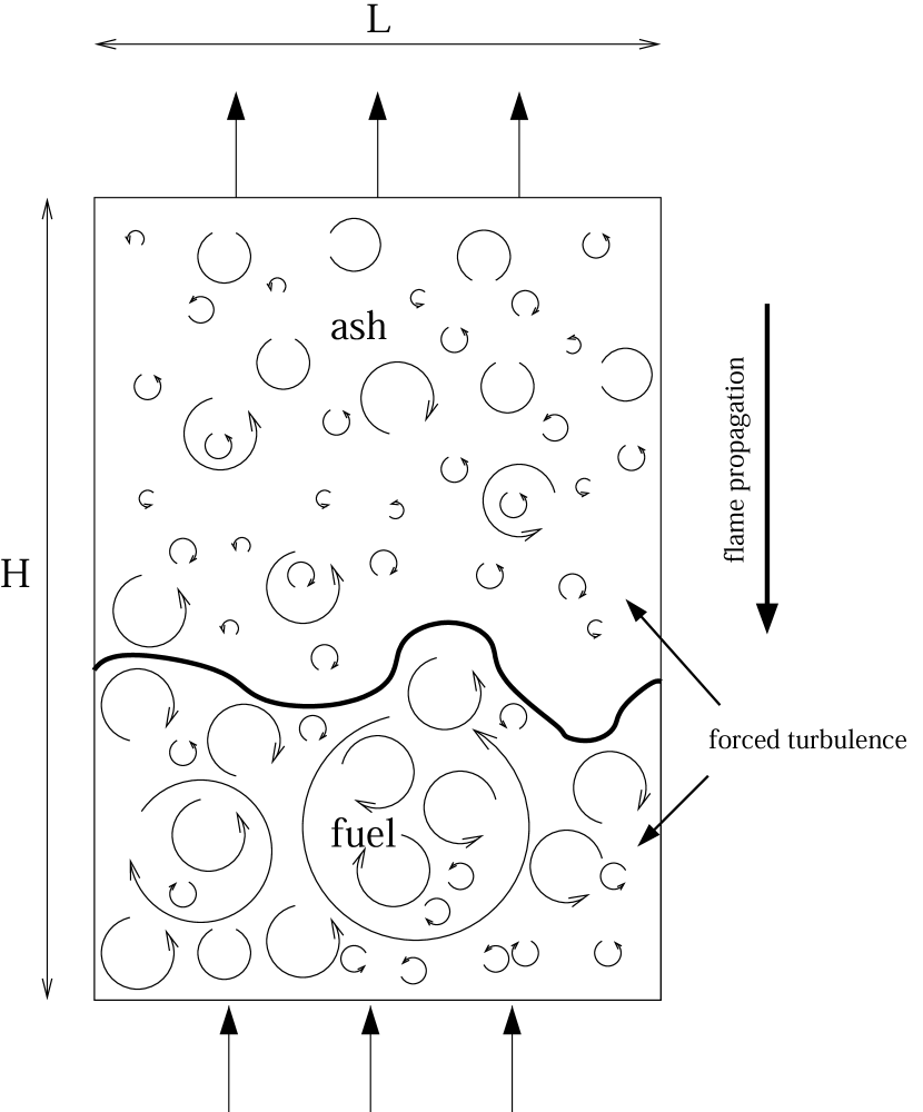
Figure 2: Diagram of the simulation setup (shown in two-dimensions for clarity). The domain is initialized with a turbulent flow and a flame is introduced into the domain, oriented to that the flame propagates downwards against the imposed mean flow. The turbulence is maintained by adding a forcing term to the momentum equations. The top and bottom boundaries are outflow and inflow, respectively. The side boundaries are periodic.

Figure 2 shows the simulation setup. The simulations were initialized with oxygen fuel in the lower part of the domain and sulphur ash in the upper part, resulting in a downward propagating flame. A high-aspect ratio domain was used, with periodic lateral boundary conditions, and outflow at the upper boundary. Due to the huge disparity in widths of carbon and oxygen flames, we are not able to capture both accurately in the same simulation. Therefore, we use carbon post-flame conditions and only burn oxygen. To recreate these condition appropriately, specifically the warm oxygen in a post carbon-flame mean velocity, we need to work in a moving frame of reference. Consequently, unlike papers I and II, a mean inflow was specified at the lower boundary to replicate the desired conditions so that an inductive oxygen flame could develop properly. Using such an inflow velocity in conjunction with the forcing term used to maintain the turbulent velocity field requires some care. It is possible to use a turbulent inflow velocity, but we have opted not to take such an approach. Instead we specify a uniform inflow and use just the forcing term itself to produce turbulence. We found that this gave satisfactory results, provided $\beta\lower 0.43057pt\hbox{\hbox to0.0pt{\raise 2.58334pt\hbox{\hskip 1.29167pt{{$\scriptscriptstyle<$}}}\hss} \kern-1.72218pt{{$\scriptscriptstyle\sim$}}}2$.

The conditions of particular interest are when $\mathrm{Da}_{16}\lower 0.43057pt\hbox{\hbox to0.0pt{\raise 2.58334pt\hbox{\hskip 1.29167pt{{$\scriptscriptstyle>$}}}\hss} \kern-1.72218pt{{$\scriptscriptstyle\sim$}}}1$. Note from figure 1 that the integral length scale is expected to be much larger than all of the turbulent flame widths under these conditions. Given that the integral length scale is approximately one-tenth of the domain width, this means that the oxygen will burn extremely close to the inlet, and certainly before the turbulence has become well-developed. To account for this, the inflow velocity, temperature and density were synthetically altered (slower, cooler and more dense, respectively) to delay oxygen burning and ensure that the flame burned approximately half-way through the domain, while maintaining conditions close to the carbon post-flame.

Oxygen Damköhler numbers of $1/3$, $1$ and $3$ were simulated to capture the potential transition. The aim is to detect the mode in which the oxygen flame is burning, specifically, what is the local turbulent oxygen flame width. However, it is difficult to measure a local turbulent flame width directly, and the widths from different modes of burning may be difficult to distinguish. Therefore, two inflow velocities were used at each Damköhler number, specifically, $\beta=1$ and $\beta=2$. This means that if the turbulent flame burns inductively, the turbulent flame widths will differ by a factor of approximately two. However, if the flames are driven by turbulent mixing, then the turbulent flame widths should be independent of $\beta$. This means that the crucial comparison required to determine the burning mode is between flames at different inflow speeds at the same Damköhler number, and direct measurements of local turbulent flame widths do not need to be evaluated, nor are comparisons of these widths necessary at different Damköhler numbers.

Simulations of one-dimensional zero-turbulence inductive flames and three-dimensional inert turbulence were first obtained, and then superimposed to initialize each calculation. Each simulation was run with a resolution of $256\times 256\times 1024$. Adaptive mesh refinement was not used. Table 1 gives the conditions for the six simulations.

4 RESULTS

Figures 3(a,b) show two-dimensional vertical slices (through three-dimensional simulations) of burning rate (left) and temperature (right) for the $\mathrm{Da}_{16}=1/3$ cases, (a) $\beta=1$ and (b) $\beta=2$. The two central panels in each figure show a snapshot of the turbulent simulations, and the narrow edge panels show the corresponding images for the (zero turbulence) inductive flames for comparison. The white lines show three relevant length scales ($l$, $l_{16}$, and $\lambda_{16}$). Note that only $l_{16}$ differs between the two cases (due to the dependence on $u_{0}$ and therefore $\beta$). Warm oxygen is being fed from below at $u_{0}=\beta\check{u}$, burns to sulphur, and leaves the domain through the top boundary. In both cases, there is a large volume of fuel burning, many times the integral length scale. It is clear that there is a high level of turbulent mixing, but the width of each flame appears to be roughly the same as the laminar inductive flame at the corresponding inflow speed. Importantly, the $\beta=2$ flame appears significantly broader than for $\beta=1$. This suggests that for $\mathrm{Da}_{16}\lower 0.43057pt\hbox{\hbox to0.0pt{\raise 2.58334pt\hbox{\hskip 1.29167pt{{$\scriptscriptstyle<$}}}\hss} \kern-1.72218pt{{$\scriptscriptstyle\sim$}}}1$, the flames burn inductively.

Figures 4(a,b) show the corresponding slices for the $\mathrm{Da}_{16}=3$ cases (the $\mathrm{Da}_{16}=1$ cases present intermediate behavior, and are not shown). Note the domain size and integral length scale are 27 times larger than figure 3, and the inflow and turbulent intensity is 3 times higher. Correspondingly, the inductive length $l_{16}$ and $\lambda$-width are relatively shorter here. In both cases, the local turbulent flame width appears to be narrower than the corresponding inductive flames shown, and is even filamentary in places. The crucial point to note here is that the local turbulent flame width does not differ significantly between the $\beta=1$ and $\beta=2$ cases. Therefore, turbulent mixing must be driving the flame propagation. If the flames were burning inductively, the $\beta=2$ case should be broader than the $\beta=1$ case. This is evidence that oxygen burns as a $\lambda$-flame for $\mathrm{Da}_{16}>1$.

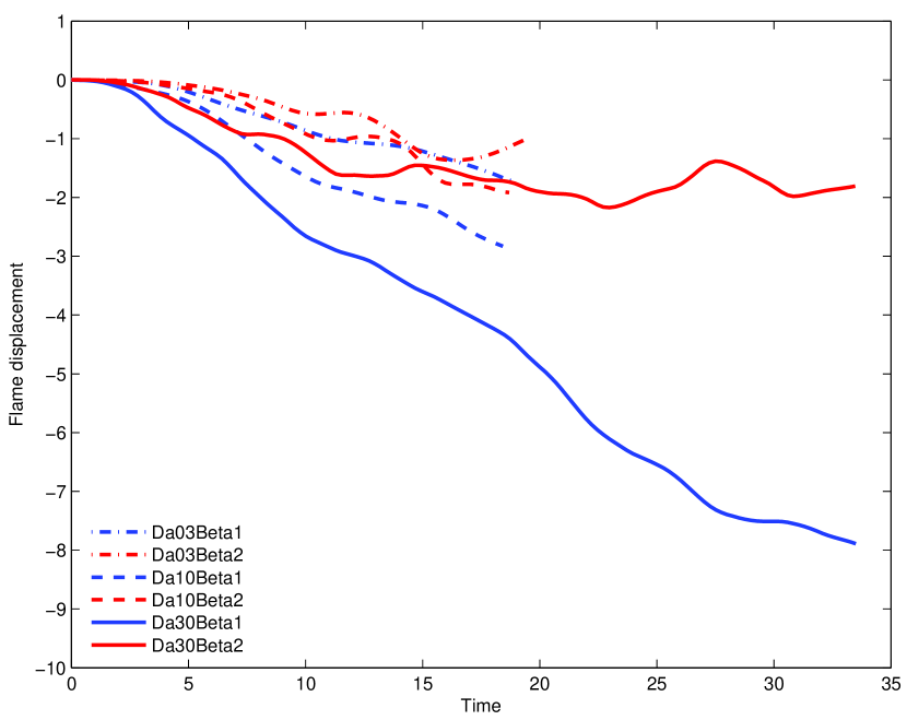
Figure 5: Flame displacement from the initial position as a function of time for all six cases. The displacement has been normalized by the integral length scale $l$, and the time has been normalized by the integral length eddy turnover time $\tau=l/\check{u}$.

An underlying assumption of the scaling analysis in section 2 is that the nuclear time scale $\tau_{16}$ is constant. This assumption, combined with a turbulent flame width narrower than $l_{16}$, suggests that the turbulent flame speed is faster than $s_{16}$ (i.e. $u_{0}=\beta\check{u}$). Figure 5 shows the flame displacement $\xi(t)=z_{0}(t)-z_{0}(0)$ from the initial position $z_{0}(0)$ as a function of time for all six cases, where the flame position has been defined as

$$z_{0}(t)=\frac{1}{A\left(\rho X_{16}\right)_{0}}\int_{V}\rho X_{16}\,\mbox{d}V.$$ (7)

The displacement has been normalized by the integral length scale $l$, and the time has been normalized by the integral length eddy turnover time $\tau=l/\check{u}$. It is clearly evident that the Da30B1 flame is indeed burning significantly faster than $u_{0}$ and propagates towards the inflow boundary; we note that it is the high Damköhler case (Da30B1) that is of particular interest.

This is an interesting consequence of turbulence-driven oxygen flame propagation, because it suggests that the conventional idea that the oxygen flame is locked at some distance (depending solely on $u_{0}$ and $\tau_{16}$) behind the carbon flame (e.g. Timmes & Woosley, 1992; Lisewski et al., 2000) cannot be the case under these conditions. For an order-of-magnitude analysis, assume the turbulent burning time scale of carbon at $\rho=2.5\times 10^{7}$ is of the order of 10^-3 s, which means the carbon $\lambda$-flame local speed and width are approximately $s_{12}^{\lambda}\approx 3\times 10^{6}$ cm/s and $\lambda_{12}\approx 3\times 10^{3}$ cm, respectively. The corresponding values for the resulting oxygen flame are $s_{16}^{\lambda}=1.13\times 10^{7}$ cm/s and $\lambda_{16}=1.81\times 10^{5}$ cm, respectively. The oxygen $\lambda$-flame is about an order of magnitude faster and two orders of magnitude thicker than the carbon flame. This suggests that the flame actually burns as a single compound carbon-oxygen flame with local flame speed and width close to that of the oxygen $\lambda$-flame.

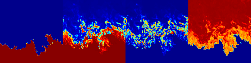
Figure 6: Two-dimensional slices through a three-dimensional simulation of a compound carbon-oxygen flame. The panels are carbon mass fraction, oxygen mass fraction, oxygen burning rate and temperature, respectively.

Figure 6 shows two-dimensional slices through a three-dimensional simulation of a compound carbon-oxygen flame where the inflow velocity and turbulent intensity were matched to case Da30B1. We emphasize that at this resolution, the carbon flame is far from being well-resolved. The simulation was initialized with a discontinuity halfway up the domain, with cold fuel under hot ash. Specifically, the fuel was at a density and temperature of $\rho=2.5\times 10^{7}$ g/cm³ and $T=6\times 10^{8}$ K, and consisted of 40% carbon and 60% oxygen. The initial ash consisted of 40% magnesium and 60% sulphur, with density and temperature of $\rho\approx 1.39\times 10^{7}$ g/cm³ and $T\approx 3.8\times 10^{9}$ K, respectively, and was allowed to evolve to the appropriate state. The figure panels are carbon mass fraction, oxygen mass fraction, oxygen burning rate and temperature, respectively. It appears that, as expected, turbulent mixing is able to drive a compound flame.

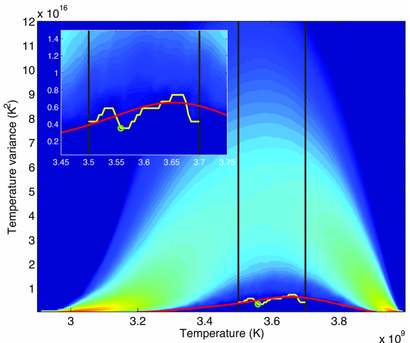
Figure 7: Joint probability density function of temperature and temperature variance evaluated using a 2.33 km cubic filter for case Da10B2. The red curve denotes the zero turbulence case filtered in the same way. The yellow line denotes the minimum variance achieved for each temperature in the range denoted by vertical black lines, over which a potential transition to detonation was proposed by Woosley et al. (2010). The green circle denotes the lowest variation that was found within this temperature range. The inset shows a zoom of the conditions of interest.

The potential transition to detonation suggested by Woosley et al. (2010) requires the formation of a region of approximately 10 km at a temperature of approximately $3.6\times 10^{9}$ K. To investigate the existence of such a region, the temperature field from the Da10B2 case averaged using a top-hat cubic filter of size $33^{3}$ cells. which corresponds to a length for each side of approximately 2.33 km. The filtered temperature and temperature variance were found at each point in space and time, and are plotted in the form of a joint probability density function in figure 7. The red curve denotes the zero turbulence case filtered in the same way. The yellow line denotes the minimum variance achieved for each temperature in the range denoted by vertical black lines, over which a potential transition to detonation was proposed by Woosley et al. (2010). Almost every point within the flame lies above the laminar profile, but there are low probability events that have a low variance within the required temperature range. However, the minimum variance over this range (denoted by the green circle) is approximately $3.5\times 10^{15}$ K². The candidate case from figure 3b of Woosley et al. (2010) has a temperature of approximately $3.67\times 10^{9}\pm 2.5\times 10^{7}$ K. Assuming a uniform distribution gives a variance of approximately $2\times 10^{14}$ K², which is an order of magnitude less than in the current simulation. Allowing for a larger range, say $\pm$1e8 K, gives a variance of approximately $3\times 10^{15}$ K². These estimates are not much lower than the laminar flame (shown by the red curve), which suggests that the turbulence does not lead to the formation of a plateau or ledge under these conditions. Furthermore, the filter size here is much smaller than required by about a factor of 4, and the variance will only increase with a larger filter size. This does not provide support for the suggests transition to detonation in oxygen for the conditions studied, but it should be noted that the simulations in Woosley et al. (2010) had a turbulent power over 15 times that used here.

5 CONCLUSIONS

The theoretical treatment of distributed carbon-burning thermonuclear flames from Aspden et al. (2010) has been applied to the trailing oxygen flames and compared with three-dimensional simulations over a range of Damköhler numbers. It was shown that for $\mathrm{Da}_{16}\lower 0.43057pt\hbox{\hbox to0.0pt{\raise 2.58334pt\hbox{\hskip 1.29167pt{{$\scriptscriptstyle<$}}}\hss} \kern-1.72218pt{{$\scriptscriptstyle\sim$}}}1$, turbulence does not greatly alter the flame from one in which the oxygen burns purely inductively. Since turbulence accelerates the carbon flame however, the width of the oxygen flame is enormously broader than in the laminar case. For $\mathrm{Da}_{16}\lower 0.43057pt\hbox{\hbox to0.0pt{\raise 2.58334pt\hbox{\hskip 1.29167pt{{$\scriptscriptstyle>$}}}\hss} \kern-1.72218pt{{$\scriptscriptstyle\sim$}}}1$, turbulence enhances heat transfer and drives flame propagations that is narrower than the corresponding zero turbulence inductive oxygen flame. This is somewhat counterintuitive as turbulence typically broadens interfaces rather than sharpening them. A consequence of burning in this limit is that the oxygen can burn faster than the inductive flame speed (but is limited by the carbon flame speed of course). Therefore, the oxygen flame does not trail behind the carbon flame (at a distance equal to the post carbon-flame velocity times the oxygen burning time scale), but burns as a compound carbon-oxygen. This suggests that a single level set is a suitable flame model for the compound flame under these conditions. Averaging the temperature field using a cubic filter suggested that the temperature variance in at the desired conditions is too high to support the potential transition to detonation in oxygen proposed in Woosley et al. (2010). However, this does not preclude this kind of transition under different conditions, such as higher turbulence or lower densities, and it should be borne in mind that only one such event would be required, and in the star there are many realizations.

Case	Da03B1	Da03B2	Da10B1	Da10B2	Da30B1	Da30B2
Damköhler number ($\mathrm{Da}_{16}$)	1/3	1/3	1	1	3	3
Inflow factor ($\beta$)	1	2	1	2	1	2
Domain width ($L$) [km]	$3.50$	$3.50$	$18.1$	$18.1$	$100$	$100$
Domain height ($H$) [km]	$14.0$	$14.0$	$72.4$	$72.4$	$400$	$400$
Integral length scale ($l$) [km]	$0.350$	$0.350$	$1.81$	$1.81$	$10.0$	$10.0$
Turbulent intensity ($\check{u}$) [km/s]	$65.4$	$65.4$	$113$	$113$	$200$	$200$
Inflow velocity ($u_{0}^{\dagger}$) [km/s]	$61.46$	$12.65$	$10.05$	$20.68$	$15.73$	$34.90$
Inflow density ($\rho_{0}^{\dagger}$) [$\times 10^{7}$ g/cm3]	$1.786$	$1.739$	$1.895$	$1.846$	$1.998$	$1.940$
Inflow temperature ($T_{0}^{\dagger}$) [$\times 10^{9}$ K]	$2.950$	$3.035$	$2.790$	$2.870$	$2.656$	$2.740$

Table 1: Simulation properties. The $\dagger$ denotes the synthetic inflow conditions that were chosen to position the laminar inductive flame close to the half-way point in the domain. The desired conditions were $\rho_{0}=1.69\times 10^{7}$ g/cm³, $T_{0}=3.14\times 10^{9}$ K and $u_{0}=\beta\check{u}$.

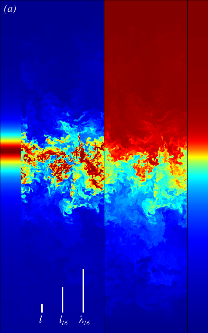
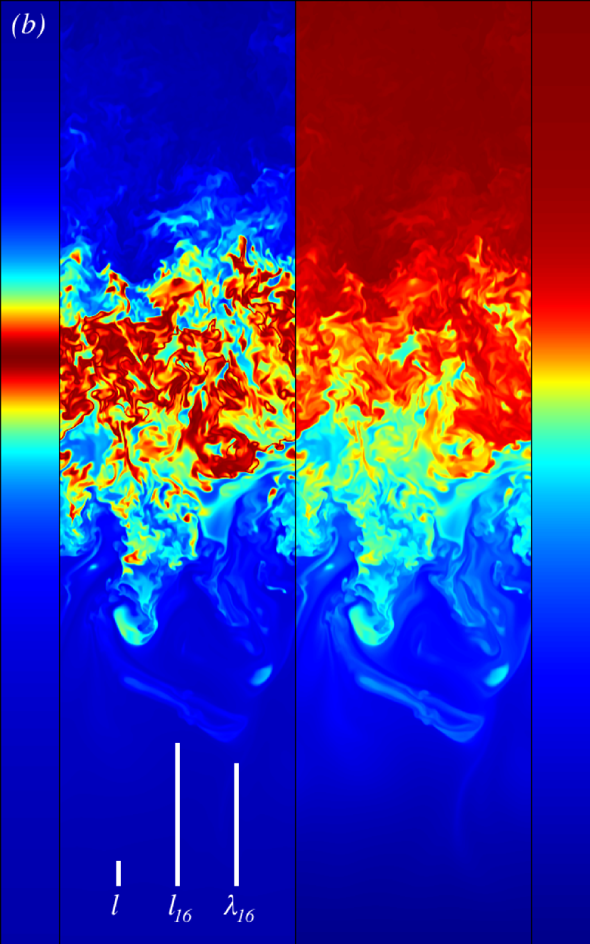
Figure 3: Two-dimensional vertical slices (through three-dimensional simulations) of burning rate (left) and temperature (right) for the $\mathrm{Da}_{16}=1/3$ cases, (a) $\beta=1$ and (b) $\beta=2$. The two central panels show a snapshot of the turbulent simulations, and the narrow edge panels show the corresponding images for the (zero turbulence) inductive flames for comparison. The white lines show three relevant length scales ($l$, $l_{16}$, and $\lambda_{16}$).

Figure 4: As figure 3 for the $\mathrm{Da}_{16}=3$ cases.

References

- Aspden et al. (2008a) Aspden, A. J., Bell, J. B., Day, M. S., Woosley, S. E., & Zingale, M. 2008a, ApJ, 689, 1173
- Aspden et al. (2010) Aspden, A. J., Bell, J. B., & Woosley, S. E. 2010, ApJ, 710, 1654
- Aspden et al. (2008b) Aspden, A. J., Nikiforakis, N., Dalziel, S. B., & Bell, J. B. 2008b, Communications in Applied Mathematics and Computational Science, 3, 101
- Bell et al. (2004) Bell, J. B., Day, M. S., Rendleman, C. A., Woosley, S. E., & Zingale, M. A. 2004, Journal of Computational Physics, 195, 677
- Caughlan & Fowler (1988) Caughlan, G. R., & Fowler, W. A. 1988, Atomic Data and Nuclear Data Tables, 40, 283, see also http://www.phy.ornl.gov/astrophysics/data/cf88/index.html
- Damköhler (1940) Damköhler, G. 1940, Z. Elektrochem, 46, 601
- Grinstein et al. (2007) Grinstein, F. F., Margolin, L. G., & Rider, W. J. 2007, Implicit Large Eddy Simulation (Cambridge University Press)
- Hoflich et al. (1995) Hoflich, P., Khokhlov, A. M., & Wheeler, J. C. 1995, ApJ, 444, 831
- Kasen et al. (2009) Kasen, D., Röpke, F. K., & Woosley, S. E. 2009, Nature, 460, 869
- Khokhlov et al. (1997) Khokhlov, A. M., Oran, E. S., & Wheeler, J. C. 1997, ApJ, 478, 678
- Kozma et al. (2005) Kozma, C., Fransson, C., Hillebrandt, W., Travaglio, C., Sollerman, J., Reinecke, M., Röpke, F. K., & Spyromilio, J. 2005, A&A, 437, 983
- Lisewski et al. (2000) Lisewski, A. M., Hillebrandt, W., Woosley, S. E., Niemeyer, J. C., & Kerstein, A. R. 2000, ApJ, 537, 405
- Mazzali et al. (2007) Mazzali, P. A., Röpke, F. K., Benetti, S., & Hillebrandt, W. 2007, Science, 315, 825
- Niemeyer & Woosley (1997) Niemeyer, J. C., & Woosley, S. E. 1997, ApJ, 475, 740
- Peters (1999) Peters, N. 1999, Journal of Fluid Mechanics, 384, 107
- Peters (2000) —. 2000, Turbulent Combustion (Cambridge University Press)
- Plewa et al. (2004) Plewa, T., Calder, A. C., & Lamb, D. Q. 2004, The Astrophysical Journal Letters, 612, L37
- Röpke (2007) Röpke, F. K. 2007, ApJ, 668, 1103
- Röpke et al. (2007) Röpke, F. K., Woosley, S. E., & Hillebrandt, W. 2007, ApJ, 660, 1344
- Timmes (2000) Timmes, F. X. 2000, ApJ, 528, 913
- Timmes & Swesty (2000) Timmes, F. X., & Swesty, F. D. 2000, ApJs, 126, 501
- Timmes & Woosley (1992) Timmes, F. X., & Woosley, S. E. 1992, ApJ, 396, 649
- Woosley et al. (2010) Woosley, S. E., Kerstein, A. R., & Aspden, A. J. 2010, ApJ, submitted
- Woosley et al. (2009) Woosley, S. E., Kerstein, A. R., Sankaran, V., Aspden, A. J., & Röpke, F. 2009, ApJ, 704, 255