Deconvolution of dynamic mechanical networks

Abstract

Time-resolved single-molecule biophysical experiments yield data that contain a wealth of dynamic information, in addition to the equilibrium distributions derived from histograms of the time series. In typical force spectroscopic setups the molecule is connected via linkers to a read-out device, forming a mechanically coupled dynamic network. Deconvolution of equilibrium distributions, filtering out the influence of the linkers, is a straightforward and common practice. We have developed an analogous dynamic deconvolution theory for the more challenging task of extracting kinetic properties of individual components in networks of arbitrary complexity and topology. Our method determines the intrinsic linear response functions of a given molecule in the network, describing the power spectrum of conformational fluctuations. The practicality of our approach is demonstrated for the particular case of a protein linked via DNA handles to two optically trapped beads at constant stretching force, which we mimic through Brownian dynamics simulations. Each well in the protein free energy landscape (corresponding to folded, unfolded, or possibly intermediate states) will have its own characteristic equilibrium fluctuations. The associated linear response function is rich in physical content, since it depends both on the shape of the well and its diffusivity—a measure of the internal friction arising from such processes like the transient breaking and reformation of bonds in the protein structure. Starting from the autocorrelation functions of the equilibrium bead fluctuations measured in this force clamp setup, we show how an experimentalist can accurately extract the state-dependent protein diffusivity using a straightforward two-step procedure.

Force spectroscopy of single biomolecules relies most commonly on atomic force microscope (AFM) CarrionVazquez99 ; Oesterhelt00 ; Wiita07 ; Khatri07 ; Greene08 ; Puchner08 ; Junker09 or optical tweezer Cecconi05 ; Woodside06 ; Woodside06b ; Greenleaf08 ; Chen09 ; Gebhardt10 techniques. By recording distance fluctuations under applied tension, these experiments serve as sensitive probes of free energy landscapes Cecconi05 ; Woodside06 ; Woodside06b ; Greenleaf08 ; Gebhardt10 , and structural transformations associated with ligand binding or enzymatic activity Wiita07 ; Puchner08 ; Junker09 . All such studies share an unavoidable complication: the signal of interest is the molecule extension as a function of time, but the experimental output signal is an indirect measure like the deflection of the AFM cantilever or the positions of beads in optical traps. The signal is distorted through all elements in the system, which in addition typically include polymeric handles such as protein domains or double-stranded DNA which connect the biomolecule to the cantilever or bead. As shown in the case of an RNA hairpin in an optical tweezer Hyeon08 , handle fluctuations lead to nontrivial distortions in equilibrium properties like the energy landscape as well as dynamic quantities like folding/unfolding rates. If an accurate estimate of the biomolecule properties is the goal, then one needs a systematic procedure to subtract the extraneous effects and recover the original signal from experimental time series data.

Static deconvolution, which operates on the equilibrium distribution functions of connected objects, is a well-known statistical mechanics procedure and has been successfully applied to recover the free energy landscape of DNA hairpins Woodside06 ; Woodside06b and more recently of a leucine zipper domain Gebhardt10 . In contrast, for dynamic properties of the biomolecule, no comprehensive deconvolution method exists. Handles and beads have their own dissipative characteristics and will tend to suppress the high-frequency fluctuations of the biomolecule and as a result distort the measured power spectrum. In the context of single-molecule pulling experiments, theoretical progress has been made in accounting for handle/bead effects on the observed unfolding transition rates Manosas2005 ; Dudko2006 ; Manosas2007 ; Dudko2008 . However, the full intrinsic fluctuation spectrum, as encoded in the time-dependent linear response function, has remained out of reach. The current work presents a systematic dynamic deconvolution procedure that fills this gap, providing a way to recover the linear response of a biomolecule integrated into a mechanical dissipative network. We work in the constant force ensemble as appropriate for optical force clamp setups with active feedback mechanisms Lang02 ; Nambiar04 or passive means Greenleaf05 ; Chen09 . While our theory is general and applies to mechanical networks of arbitrary topology, we illustrate our approach for the specific experimental setup of Ref. Gebhardt10 : a protein attached to optically trapped beads through dsDNA handles. The only inputs required by our theory are the autocorrelation functions of the bead fluctuations in equilibrium. We demonstrate how the results from two different experimental runs—one with the protein, and one without—can be combined to yield the protein linear response functions.

We apply this two-step procedure on a force clamp setup simulated through Brownian dynamics, and verify the accuracy of our dynamic deconvolution method. Knowledge of mechanical linear response functions forms the basis of understanding viscoelastic material properties; the protein case is particularly interesting because every folding state, i.e. each well in the free energy landscape, will have its own spectrum of equilibrium fluctuations, and hence a distinct linear response function. Two key properties determine this function: the shape of the free energy around the minimum, and the local diffusivity. The latter has contributions both from solvent drag and the effective roughness of the energy landscape—internal friction due to molecular torsional transitions and the formation and rupture of bonds between different parts of the peptide chain. The diffusivity profile is crucial for getting a comprehensive picture of protein folding kinetics and arguably it is just as important as the free energy landscape itself for very fast folding proteins Cellmer08 ; Best10 ; Hinczewski10 . Our dynamic deconvolution theory provides a promising route to extract this important protein characteristic from future force clamp studies.

I Results and discussion

I.1 Force clamp experiments and static deconvolution

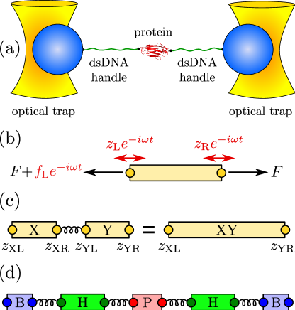
Figure 1: (a) Double optical tweezer force clamp setup for the study of equilibrium protein dynamics, with soft traps approximating a constant tension $F$. (b) To define linear response functions, consider an individual component at tension $F$. A small additional oscillatory force $f_{\text{L}}\exp(-i\omega t)$ applied at the left end leads to endpoint oscillations with amplitudes $z_{L}=J_{\text{self,L}}(\omega)f_{\text{L }}$ and $z_{R}=J_{\text{cross}}(\omega)f_{\text{L}}$ which defines the self and cross response functions. (c) Two objects X and Y connected in series behave as a composite object XY whose response functions can be derived through simple rules (Eq. (2)) from the individual X and Y response functions. (d) Schematic representation of the optical tweezer setup consisting of beads (B), double-stranded DNA handles (H) and protein (P), with connecting springs.

As a representative case, in this paper we consider the double trap setup shown in Fig. 1(a), which typically involves two optically-trapped polystyrene beads of radius $\sim{\cal O}(10^{2}\>\text{nm})$, two double-stranded DNA handles, each $\sim{\cal O}(10^{2}\>\text{nm})$, attached to a protein in the centerGebhardt10 . For fixed trap positions and sufficiently soft trapping potentials, the entire system will be in equilibrium at an approximately constant tension $F$. We are interested in a force regime ($F\gtrsim 10$ pN in the system under consideration) where the handles are significantly stretched in the direction parallel to the applied force (chosen as the $z$ axis), and rotational fluctuations of the handle-bead contact points are small. Since the experimental setup is designed to measure the $z$ separation of the beads as a function of time, we focus entirely on the dynamic response of the system along the $z$ direction. However, the methods below can be easily generalized to the transverse response as well. Though we consider only a passive measurement system in our analysis, an active feedback loop that minimizes force fluctuations can also be incorporated, as an additional component with its own characteristic dynamic response (with the added complication that the response of the feedback mechanism would have to be independently determined).

To set the stage for our dynamic deconvolution theory, we first illustrate the static deconvolution for two objects X and Y connected in series under constant tension $F$, e.g. a protein and a handle. Let ${\cal P}^{\text{X}}(z)$ and ${\cal P}^{\text{Y}}(z)$ be the constant-force probability distributions for each of these objects having end-to-end distance $z$. The total system end-to-end distribution is given by ${\cal P}^{\text{XY}}(z)=\int dz^{\prime}{\cal P}^{\text{X}}(z^{\prime}){\cal P}^{\text{Y}}(z-z^{\prime})$. In terms of the Fourier-transformed distributions, this can be stated simply through the ordinary convolution theorem, $\tilde{\cal P}^{\text{XY}}(k)=\tilde{\cal P}^{\text{X}}(k)\tilde{{\cal P}}^{\text{Y}}(k)$. If ${\cal P}^{\text{XY}}$ is derived from histograms of the experimental time series, and if ${\cal P}^{\text{Y}}$ can be estimated independently (either from an experiment without the protein, or through theory), then we can invert the convolution relation to solve for the protein distribution ${\cal P}^{\text{X}}$ and thus extract the folding free energy landscape. A similar approach works for multiple objects in series or in parallel.

I.2 Dynamic response functions

Before we consider dynamic networks, we define the linear response of a single object under constant stretching force $F$ along the $z$ direction, as shown in Fig. 1(b). Imagine applying an additional small oscillatory force $f_{\text{L}}\exp(-i\omega t)$ along the $z$ axis to the left end. The result will be small oscillations $z_{\text{L}}\exp(-i\omega t)$ and $z_{\text{R}}\exp(-i\omega t)$ of the two ends around their equilibrium positions. The complex amplitudes $z_{\text{L}}$ and $z_{\text{R}}$ are related to $f_{\text{L}}$ through linear response: $z_{\text{L}}=J_{\text{self,L}}(\omega)f_{\text{L}}$, $z_{\text{R}}=J_{\text{cross}}(\omega)f_{\text{L}}$, defining the self response function $J_{\text{self,L}}(\omega)$ of the left end and the cross response function $J_{\text{cross}}(\omega)$. If the oscillatory force is applied instead at the right end, the response takes the form: $z_{\text{R}}=J_{\text{self,R}}(\omega)f_{\text{R}}$, $z_{\text{L}}=J_{\text{cross}}(\omega)f_{\text{R}}$. Note that since the object is in general asymmetric, $J_{\text{self,L}}(\omega)$ and $J_{\text{self,R}}(\omega)$ are distinct functions. However, there is only a single cross response (in the absence of time-reversal breaking effects such as magnetic fields Landau ). For the purposes of dynamic deconvolution of a network, these three response functions contain the complete dynamical description of a given component and are all we need. It is convenient to define the end-to-end response function $J_{\text{ee}}(\omega)$, with $z_{\text{R}}-z_{\text{L}}=J_{\text{ee}}(\omega)f$, where the oscillatory force $f\exp(-i\omega t)$ is applied simultaneously to both ends of the object in opposite directions. This response turns out to be a linear combination of the other functions: $J_{\text{ee}}=J_{\text{self,L}}+J_{\text{self,R}}-2J_{\text{cross}}$.

As an illustration we take the simplest, non-trivial example: two spheres with different mobilities $\mu_{\text{L}}$ and $\mu_{\text{R}}$ connected by a harmonic spring of stiffness $k$. In water we are typically in the low Reynolds number regime and an overdamped dynamical description is appropriate. If an oscillating force of amplitude $f_{\text{L}}$ is applied to the left sphere, its velocity will oscillate with the amplitude $-i\omega z_{\text{L}}=\mu_{\text{L}}(f_{\text{L}}+k[z_{\text{R}}-z_{\text{L}}])$, while the velocity amplitude of the right sphere is given by $-i\omega z_{\text{R}}=-\mu_{\text{R}}k[z_{\text{R}}-z_{\text{L}}]$. Using the above definitions of the response functions we obtain

$$\begin{split}J_{\text{self,L}}&=\frac{\mu_{\text{L}}(\omega+i\mu_{\text{R}}k)}{\omega(\mu k-i\omega)},\>\;J_{\text{cross}}=\frac{i\mu_{\text{L}}\mu_{\text{R}}k}{\omega(\mu k-i\omega)},\\ J_{\text{ee}}&=\frac{\mu}{\mu k-i\omega},\end{split}$$ (1)

where $\mu=\mu_{\text{L}}+\mu_{\text{R}}$. By symmetry $J_{\text{self,R}}$ is the same as $J_{\text{self,L}}$ with subscripts L and R interchanged. The end-to-end response $J_{\text{ee}}$ has a standard Lorentzian form. For more realistic force transducers, such as semiflexible polymers, $J_{\text{ee}}$ will later be written as a sum of Lorentzians reflecting the polymer normal modes. Note that when $k=0$, and the spheres no longer interact, $J_{\text{self,L}}=i\mu_{\text{L}}/\omega$, the standard result for a diffusing sphere, and $J_{\text{cross}}=0$, as expected, since there is no force transmission from one sphere to the other.

Though all the linear response functions are defined in terms of an external oscillatory force, in practice one does not need to actually apply such a force to determine the functions experimentally. As described in the two-step deconvolution procedure below, one can extract them from measurements that are far easier to implement in the lab, namely by calculating autocorrelation functions of equilibrium fluctuations.

I.3 Dynamic convolution of networks

Based on the notion of self and cross response functions, we now consider the dynamics of composites. We explicitly display the convolution formulas for combining two objects in series and in parallel; by iteration the response of a network of arbitrary topology and complexity can thus be constructed. As shown in Fig. 1(c), assume we have two objects X and Y connected by a spring. X is described by response functions $J^{\text{X}}_{\text{self,L}}$, $J^{\text{X}}_{\text{self,R}}$, and $J^{\text{X}}_{\text{cross}}$, and we have the analogous set for Y. The internal spring is added for easy evaluation of the force acting between the objects, it is eliminated at the end by sending its stiffness to infinity. We would like to know the response functions of the composite XY object, $J^{\text{XY}}_{\text{self,X}}$, $J^{\text{XY}}_{\text{self,Y}}$, and $J^{\text{XY}}_{\text{cross}}$, where the X and Y labels correspond to left and right ends, respectively. The rules (with full derivation in the Supplementary Information (SI)) read

$$\begin{split}J^{\text{XY}}_{\text{self,X}}&=J^{\text{X}}_{\text{self,L}}-\frac{\left(J^{\text{X}}_{\text{cross}}\right)^{2}}{J^{\text{X}}_{\text{self,R}}+J^{\text{Y}}_{\text{self,L}}},\\ J^{\text{XY}}_{\text{self,Y}}&=J^{\text{Y}}_{\text{self,R}}-\frac{\left(J^{\text{Y}}_{\text{cross}}\right)^{2}}{J^{\text{X}}_{\text{self,R}}+J^{\text{Y}}_{\text{self,L}}},\\ J^{\text{XY}}_{\text{cross}}&=\frac{J^{\text{X}}_{\text{cross}}J^{\text{Y}}_{\text{cross}}}{J^{\text{X}}_{\text{self,R}}+J^{\text{Y}}_{\text{self,L}}}.\end{split}$$ (2)

The rules for connecting two objects in parallel are more straightforward and read $G^{\text{XY}}_{\alpha}=G^{\text{X}}_{\alpha}+G^{\text{Y}}_{\alpha}$, where $\alpha$ is any one of the function categories (self, cross or end-to-end), and $G$ denote the inverse response functions. One particularly relevant realization for parallel mechanical pathways are long-range hydrodynamic coupling effects, that experimentally act between beads and polymer handles in the force clamp setup. We derive the parallel rule and show an example hydrodynamic application in the SI. For simplicity, however, we will concentrate in our analysis on serial connections. To proceed, if we set X=H and Y=B, we can obtain the response functions of the composite handle-bead (HB) object, $J^{\text{HB}}_{\alpha}$, if we know the response functions of the bead and handle separately. Our full system in Fig. 1(d) is just the protein sandwiched between two HB components (oriented such that the handle ends of each HB are attached to the protein). The total system response functions (denoted by “2HB+P”) in terms of the individual protein and HB functions result by iterating the pair convolution in Eq. (2) twice. In particular, the end-to-end response $J^{\text{2HB+P}}_{\text{ee}}$ is given by:

$$J^{\text{2HB+P}}_{\text{ee}}=2J^{\text{HB}}_{\text{self,B}}-\frac{2(J^{\text{HB}}_{\text{cross}})^{2}}{J^{\text{HB}}_{\text{self,H}}+J^{\text{P}}_{\text{ee}}/2}.$$ (3)

This is a key relation, since we show below that both $J^{\text{2HB+P}}_{\text{ee}}$ and the three HB response functions $J^{\text{HB}}_{\text{self,H}}$, $J^{\text{HB}}_{\text{self,B}}$, $J^{\text{HB}}_{\text{cross}}$ can be derived from force clamp experimental data. Hence Eq. (3) allows us to estimate the unknown protein response function $J^{\text{P}}_{\text{ee}}$.

We note a striking similarity to the signal processing scenario Oppenheim , where the output of a linear time-invariant (LTI) network (e.g. an RLC electric circuit) is characterized through a “transfer function”. For such networks, combination rules in terms of serial, parallel, and feedback loop motifs exist. The result for $J^{\text{XY}}_{\text{self,X}}$ in Eq. (2) can be seen in a similar light: the first term is the self-response $J^{\text{X}}_{\text{self,X}}$ of object X which is independent of the presence of object Y. The rational function in the second term is the “feedback” due to X interacting with Y. As expected, if the cross-response $J^{\text{X}}_{\text{cross}}$ connecting the two ends of X is turned off, this feedback disappears. In analogy to the transfer function theory for LTI systems, our convolution rules form a comprehensive basis to describe the response of an arbitrarily complicated network inside a force clamp experiment. And like the transfer functions which arise out of LTI feedback loops, the convolution of interacting components consists of a nonlinear combination of the individual response functions. The rational functions due to the feedback of mechanical perturbations across the connected elements are non-trivial, but can be exactly accounted for via iteration of the convolution rules.

I.4 Two-step dynamic deconvolution yields protein dynamic properties

To illustrate our theory, we construct a two-step procedure to analyze the experimental system in Fig. 1(a), with the ultimate goal of determining dynamic protein properties in the force clamp. Under a constant force $F$, the protein extension will fluctuate around a mean corresponding to a folded or unfolded state. Though it has been demonstrated that under appropriately tuned forces the protein can show spontaneous transitions between folded and unfolded states, we for the moment neglect this more complex scenario. (In the SI we analyze simulation results for a protein exhibiting a double-well free energy, where the two states can be analyzed independently by pooling data from every visit to a given well; the same idea can be readily extended to analyze time series data from proteins with one or more intermediate states.) We consider the protein dynamics as diffusion of the reaction coordinate $z^{\text{P}}_{\text{ee}}$ (the protein end-to-end distance) in a free energy landscape $U_{\text{P}}(z^{\text{P}}_{\text{ee}})$. The end-to-end response function $J^{\text{P}}_{\text{ee}}$ reflects the shape of $U_{\text{P}}$ around the local minimum, and the internal protein friction (i.e the local mobility), which is the key quantity of interest. The simplest example is a parabolic well at position $z^{\text{P}}_{\text{ee}}=z_{0}$, namely $U_{\text{P}}(z^{\text{P}}_{\text{ee}})=U_{\text{P}}(z_{0})+(1/2)k_{\text{P}}(z^{\text{P}}_{\text{ee}}-z_{0})^{2}$. If we assume the protein mobility $\mu_{\text{P}}$ is approximately constant within this state, the end-to-end response is given by

$$J^{\text{P}}_{\text{ee}}(\omega)=\frac{\mu_{\text{P}}}{\mu_{\text{P}}k_{\text{P}}-i\omega}$$ (4)

which has the same Lorentzian form as the harmonic two-sphere end-to-end response in Eq. (1). Depending on the resolution and quality of the experimental data, more complex fitting forms may be substituted, including anharmonic corrections and non-constant diffusivity profiles (an example of these is given in the two-state protein case analyzed in the SI). However for practical purposes Eq. (4) is a good starting point.

An experimentalist seeking to determine $J^{\text{P}}_{\text{ee}}(\omega)$ would carry out the following two-step procedure:

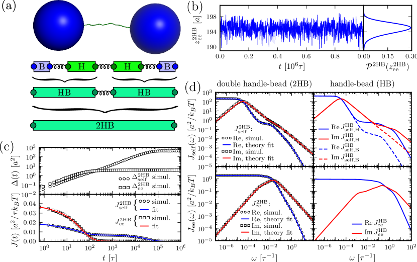
Figure 2: The first step in the deconvolution procedure, needed to to determine the handle-bead response $J^{\text{HB}}$: analysis of the optical tweezer system without the protein. (a) From top to bottom: a Brownian dynamics simulation snapshot; schematic representation of the system; after the first convolution step handles and beads are grouped into composite handle-bead (HB) objects; after the second convolution step the full system (“2HB”) constitutes a single object. (b) Part of the simulation time series for the total system end-to-end distance $z^{\text{2HB}}_{\text{ee}}$. The time series yields the equilbrium probability distribution ${\cal P}^{\text{2HB}}(z^{\text{2HB}}_{\text{ee}})$ shown on the right. (c) Top: the MSD functions $\Delta^{\text{2HB}}_{\text{self}}(t)$ and $\Delta^{\text{2HB}}_{\text{ee}}(t)$ (Eq. (5)) calculated from the simulation; bottom: the time-domain response functions $J^{\text{2HB}}_{\text{self}}(t)=(\beta/2)d\Delta^{\text{2HB}}_{\text{self}}(t)/dt$, $J^{\text{2HB}}_{\text{ee}}(t)=(\beta/2)d\Delta^{\text{2HB}}_{\text{ee}}(t)/dt$. Simulation results (symbols) are numerical derivatives of the curves in the top panel. The solid lines are a 5-exponential fit to the simulation results. (d) Left column: the real and imaginary parts of the $J^{\text{2HB}}$ self and end-to-end response functions. Simulation results (symbols) are just the Fourier transforms of the multi-exponential fits in (c). Theoretical fitting results according to Eq. (2) and based on HB functions $J^{\text{HB}}$ are shown as solid lines. Right column: the HB response functions, as determined by the theoretical fitting to the full system data.

First step: Make a preliminary run using a system without the protein (just two beads and two handles, as illustrated in Fig. 2(a)). As described in the Materials and Methods (MM), time derivatives of autocorrelation functions calculated from the bead position time series can be Fourier transformed to directly give $J^{\text{2HB}}_{\text{self}}$ and $J^{\text{2HB}}_{\text{cross}}$. The convolution rules in Eq. (2) relate $J^{\text{2HB}}_{\text{self}}$ and $J^{\text{2HB}}_{\text{cross}}$ to the bead/handle response functions, $J^{\text{HB}}_{\text{self}}$ and $J^{\text{HB}}_{\text{cross}}$, which via another application of Eq. (2) are related to the response functions of a single bead and a single handle. The bead functions $J^{\text{B}}_{\text{self}}$ and $J^{\text{B}}_{\text{cross}}$ depend solely on known experimental parameters (MM), leaving only the handle functions $J^{\text{H}}_{\text{self}}$ and $J^{\text{H}}_{\text{cross}}$ as unknowns in the convolution equations. Choosing an appropriate fitting form, determined by polymer dynamical theory (see MM), we can straightforwardly determine $J^{\text{H}}_{\text{self}}$ and $J^{\text{H}}_{\text{cross}}$.

Second step: Make a production run with the protein. Eq. (3) relates the resulting end-to-end response $J^{\text{2HB+P}}_{\text{ee}}$, extracted from the experimental data, to the response of the protein alone $J^{\text{P}}_{\text{ee}}$. Since the first step yielded the composite handle-bead functions $J^{\text{HB}}_{\text{self,H}}$, $J^{\text{HB}}_{\text{self,B}}$, $J^{\text{HB}}_{\text{cross}}$ which appear in Eq. (3), the only unknown is $J^{\text{P}}_{\text{ee}}$. We can thus solve for the parameters $\mu_{\text{P}}$ and $k_{\text{P}}$ which appear in Eq. (4).

This two-step procedure can be repeated at different applied tensions, revealing how the protein properties (i.e. the intramolecular interactions that contribute to the diffusivity $\mu_{\text{P}}$) depend on force. Even analyzing the unfolded state of the protein might yield interesting results: certain forces might be strong enough to destroy the tertiary structure, but not completely destabilize the secondary structure, which could transiently refold and affect $\mu_{\text{P}}$.

I.5 Simulations validate the deconvolution technique

To demonstrate the two-step deconvolution procedure in a realistic context, we perform Brownian dynamics simulations mimicking a typical force clamp experiment: two beads that undergo rotational and translational fluctuations are trapped in 3D harmonic potentials and connected to two semiflexible polymers which are linked together via a potential function that represents the protein folding landscape (see MM for details). We ignore hydrodynamic effects which can easily be accounted for through parallel coupling pathways, as mentioned above.

We begin with the first step of the deconvolution procedure. A snapshot of the simulation system, two handles and two beads without a protein, is shown in Fig. 2(a). A representative segment of the $z^{\text{2HB}}_{\text{ee}}(t)$ time series is shown in Fig. 2(b). Equilibrium analysis of the time series yields the end-to-end distribution ${\cal P}^{\text{2HB}}(z^{\text{2HB}}_{\text{ee}})$, which is useful for extracting static properties of the protein like the free energy landscape: when the protein is added to the system, the total end-to-end distribution is just a convolution of the 2HB and protein distributions. (The asymmetry of ${\cal P}^{\text{2HB}}$ seen in Fig. 2(b) arises from the semiflexible nature of the handles.) As described in MM, we use the time series to calculate self and end-to-end MSD curves $\Delta_{\text{self}}^{\text{2HB}}(t)$ and $\Delta_{\text{ee}}^{\text{2HB}}(t)$ [Fig. 2(c)] whose derivatives are proportional to the time-domain response functions $J^{\text{2HB}}_{\text{self}}(t)$ and $J^{\text{2HB}}_{\text{ee}}(t)$. The multi-exponential fits to these functions are illustrated in Fig. 2(c), and their analytic Fourier transforms plotted in the left column of Fig. 2(d). We thus have a complete dynamical picture of the 2HB system response. However, in order to use Eq. (3) to extract the protein response, we first have to determine the handle-bead response functions $J^{\text{HB}}_{\alpha}$. Although a general fit of $J^{\text{HB}}_{\alpha}$ is possible, it is useful to apply the knowledge about the bead parameters and symmetry properties of the handle response. The handle parameters (the set $\{k^{\text{H}}_{m},\mu_{m}^{\text{H}}\}$ in MM Eq. (7)) are the only unknowns in the three HB response functions: $J^{\text{HB}}_{\text{self,H}}$, $J^{\text{HB}}_{\text{self,B}}$, and $J^{\text{HB}}_{\text{ee}}$. Note that the handle-bead object is clearly asymmetric, so the self response will be different at the handle (H) and bead (B) end. Convolving two HB objects according to Eq. (2) and fitting the handle parameters to the simulation results for $J^{\text{2HB}}_{\text{self}}(\omega)$ and $J^{\text{2HB}}_{\text{ee}}(\omega)$ leads to the excellent description shown as solid lines on the left in Fig. 2(d). The handle parameters derived from this fitting completely describe the HB response functions $J^{\text{HB}}_{\alpha}$, shown in the right column of Fig. 2(d). The HB response curves reflect their individual components: there is a low frequency peak/plateau in the imaginary/real part of the HB self response, related to the slow relaxation of the bead in the trap. The higher frequency contributions are due to the handles, and as a result they are more prominent in the self response of the handle end than of the bead end. There is a similarly non-trivial structure in the end-to-end response, due to the complex interactions between the handle normal modes and the fluctuations of the trapped bead (see SI for more details).

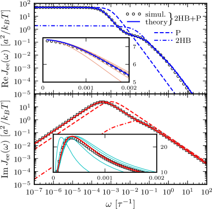
Figure 3: Real (top) and imaginary (bottom) parts of the total end-to-end response $J^{\text{2HB+P}}_{\text{ee}}(\omega)$ of an optical tweezer system with the protein modeled as a single parabolic potential well ($k_{\text{P}}=0.02$ $k_{B}T/a^{2}$, $\mu_{\text{P}}=0.05\mu_{0}$). Symbols are simulation results, and the solid line is the theoretical prediction, based on the convolution of the protein response $J^{\text{P}}_{\text{ee}}(\omega)$ with the HB response functions $J^{\text{HB}}$ of Fig. 2(d) according to Eq. (3). For comparison, $J^{\text{P}}_{\text{ee}}(\omega)$ (dashed line) and $J^{\text{2HB}}_{\text{ee}}(\omega)$ (dot-dashed line) are also included. Insets: to show the sensitivity of the theoretical fitting, zoomed-in sections of $J^{\text{2HB+P}}_{\text{ee}}(\omega)$ near the maxima of the real (top) and imaginary (bottom) components. Both simulation (symbols) and theoretical (blue/red curve) results are plotted. The thin pink/cyan curves are theoretical results with $\mu_{\text{P}}$ different from the true value: from left to right, $\mu_{\text{P}}=0.01$, $0.03$, $0.07$, $0.09\mu_{0}$.

The double-HB end-to-end distribution in Fig. 2(b) and the HB response functions in Fig. 2(d) are all we need to know about the optical tweezer system: the equilibrium end-to-end distribution and linear response of any object which we now put between the handles can be reconstructed. We will illustrate this using a toy model of a protein. In our simulations for the second step, we use a parabolic potential $U_{\text{P}}$ with $U^{\prime\prime}_{\text{P}}(z)=k_{\text{P}}=0.02$ $k_{B}T/a^{2}$, and a fixed mobility $\mu_{\text{P}}=0.05\mu_{0}$. Here $a=1$ nm and $\mu_{0}=1/6\pi\eta a$, where $\eta$ is the viscosity of water. This leads to the single-Lorentzian response function $J^{\text{P}}_{\text{ee}}$ of Eq. (4). If this exact theoretical form of $J^{\text{P}}_{\text{ee}}$ is convolved with the HB response functions from the first step according to Eq. (3), we get the result in Fig. 3: very close agreement with $J^{\text{2HB+P}}_{\text{ee}}$ directly derived from the simulated time series data. For comparison we also plot the separate end-to-end responses of the protein alone (P) and the double-HB setup without a protein (2HB). As expected $J^{\text{2HB+P}}_{\text{ee}}$ differs substantially from both of these as correctly predicted by the convolution theory. The effect of adding handles and beads to the protein is to shift the peak in the imaginary part of the total system response to lower frequencies. Additionally, we see in $J^{\text{2HB+P}}_{\text{ee}}$ the contributions of the handle and bead rotational motions, which are dominant at higher frequencies. The sensitivity of the theoretical fit is shown in the insets of Fig. 3: zooming in on the maxima of $\text{Re}\,J^{\text{2HB+P}}_{\text{ee}}$ and $\text{Im}\,J^{\text{2HB+P}}_{\text{ee}}$, we plot the true theoretical prediction (red/blue curves) and results with $\mu_{\text{P}}$ shifted away from the the true value (thin pink/cyan curves). In fact if $k_{\text{P}}$ and $\mu_{\text{P}}$ are taken as free parameters, numerical fitting to the simulation $J^{\text{2HB+P}}_{\text{ee}}$ yields accurate values of: $\mu_{\text{P}}=0.050\mu_{0}$ and $k_{\text{P}}=0.0199$ $k_{B}T/a^{2}$. Examples of successful deconvolution with other values of the intrinsic protein parameters are given in the double-well free energy analysis in the SI.

In practice, any theoretical approach must take into consideration instrumental limitations: most significantly, there will be a minimum possible interval $t_{\text{s}}$ between data collections, related to the time resolution of the measuring equipment. The deconvolution theory can always be applied in the frequency range up to $\omega_{s}=1/t_{s}$. Whatever physical features of any component in the system that fall within this range, can be modeled and extracted, without requiring inaccessible knowledge of fluctuation modes above the frequency cutoff $\omega_{s}$. In the SI, we illustrate this directly on the toy protein discussed above, coarse-graining the simulation time series to 0.01 ms intervals, mimicking the equipment resolution used in Ref. Gebhardt10 . The characteristic frequency of the protein within the tweezer setup falls within the cutoff, and hence our two-step deconvolution procedure can still be applied to yield accurate best-fit results for the protein parameters. The SI also includes a discussion of other experimental artifacts—white noise, drift, and effective averaging of the time series on the time scale $t_{s}$—and shows how to adapt the procedure to correct for these effects.

II Conclusion

Dynamic deconvolution theory allows us to extract the response functions of a single component from the overall response of a multicomposite network. The theory is most transparently formulated in the frequency domain, and provides the means to reverse the filtering influence of all elements that are connected to the component of interest. From the extracted single-component response function, dynamic properties such as the internal mobility or friction can be directly deduced. At the heart of our theory stands the observation that the response of any component in the network is completely determined by three functions, namely the cross response and the two self responses, which are in general different at the two ends. The response of any network can be predicted by repeated iteration of our convolution formulas for serial and parallel connections. Self-similar or more complicated network topologies, as occur in visco-elastic media, can thus be treated as well. We demonstrate the application of our deconvolution theory for a simple mechanical network that mimics a double-laser-tweezer setup, but the underlying idea is directly analogous to the signal processing rules which describe other scalar dynamic networks, such as electrical circuits or chemical reaction pathways in systems biology Muzzey09 . We finally point out that dynamic convolution also occurs in FRET experiments on proteins where polymeric linkers and conformational fluctuations of fluorophores, as well as the internal fluorescence dynamics, modify the measured dynamic fluctuation spectrum Gopich09 ; Chung10 ; Chung10b . The experimental challenge in the future will thus be to generate time-series data for single biomolecules with a sufficient frequency range in order to perform an accurate deconvolution. For this a careful matching of the relevant time and spatial scales of the biomolecule under study and the corresponding scales of the measuring device (handles as well as beads) is crucial, for which our theory provides the necessary guidance.

III Materials and Methods

III.1 Determining the total system response from the experimental time series

A key step in the experimental analysis is to obtain the system response functions $J_{\text{self}}(\omega)$ and $J_{\text{cross}}(\omega)$ from the raw data (which can either be the double handle-bead system with or without a protein). This data consists of two time series $z_{\text{B,L}}(t)$ and $z_{\text{B,R}}(t)$ for the left/right bead positions from which we calculate the mean square displacement (MSD) functions

$$\begin{split}\Delta_{\text{self}}(t)&=\frac{1}{2}\langle(z_{\text{B,L}}(t)-z_{\text{B,L}}(0))^{2}\rangle\\ &\qquad+\frac{1}{2}\langle(z_{\text{B,R}}(t)-z_{\text{B,R}}(0))^{2}\rangle,\\ \Delta_{\text{ee}}(t)&=\langle(z_{\text{ee}}(t)-z_{\text{ee}}(0))^{2}\rangle,\end{split}$$ (5)

where $z_{\text{ee}}(t)=z_{\text{B,R}}(t)-z_{\text{B,L}}(t)$, and we have averaged the self MSD of the two endpoints because they are identical by symmetry. Calculating the MSD functions is equivalent to finding the autocorrelation of the time series: for example, if $R_{\text{ee}}(t)=\langle z_{\text{ee}}(t)z_{\text{ee}}(0)\rangle$ is the end-to-end autocorrelation, the MSD $\Delta_{\text{ee}}(t)$ is simply given by $\Delta_{\text{ee}}(t)=2(R_{\text{ee}}(0)-R_{\text{ee}}(t))$.
From the fluctuation-dissipation theorem Landau , the time-domain response functions $J_{\text{self}}(t)$ and $J_{\text{ee}}(t)$ are related to the derivatives of the MSD functions: $J_{\text{self}}(t)=(\beta/2)d\Delta_{\text{self}}(t)/dt$, $J_{\text{ee}}(t)=(\beta/2)d\Delta_{\text{ee}}(t)/dt$, where $\beta=1/k_{B}T$. To get the Fourier-space response, the time-domain functions can be numerically fit to a multi-exponential form, for example $J_{\text{self}}(t)=\sum_{i}C_{i}\exp(-\Lambda_{i}t)$. In our simulation examples typically 4-5 exponentials are needed for a reasonable fit. Once the parameters $C_{i}$ and $\Lambda_{i}$ are determined, the expression can be exactly Fourier-transformed to give the frequency-domain response function, $J_{\text{self}}(\omega)=\sum_{i}C_{i}/(\Lambda_{i}-i\omega)$. An analogous procedure is used to obtain $J_{\text{ee}}(\omega)$. The cross response follows as $J_{\text{cross}}=J_{\text{self}}-J_{\text{ee}}/2$. The power spectrum associated with a particular type of fluctuation, for example the end-to-end spectrum $R_{\text{ee}}(\omega)$ (defined as the the Fourier transform of the autocorrelation), is just proportional to the imaginary part of the corresponding response function: $R_{\text{ee}}(\omega)=(2k_{B}T/\omega)\text{Im}\,J_{\text{ee}}(\omega)$.

III.2 Bead response functions

The response functions of the beads in the optical traps are the easiest to characterize, since they depend on quantities which are all known by the experimentalist: the trap stiffness $k_{\text{trap}}$, bead radius $R$, mobility $\mu_{\text{B}}=1/6\pi\eta R$, and rotational mobility $\mu_{\text{rot}}=1/8\pi\eta R^{3}$. Here $\eta$ is the viscosity of water. For each bead the three response functions can be defined as described above, with the two “endpoints” being the handle-attachment point on the bead surface ($z_{S}$) and the bead center ($z_{B}$). The latter point is significant because this position is what is directly measured by the experiment. For the case of large $F$, where the rotational diffusion of the bead is confined to small angles away from the $z$ axis, the response functions are:

$$\begin{split}J^{\text{B}}_{\text{self,B}}(\omega)&=J^{\text{B}}_{\text{cross}}(\omega)=\frac{\mu_{\text{B}}}{\mu_{\text{B}}k_{\text{trap}}-i\omega},\\ J^{\text{B}}_{\text{self,S}}(\omega)&=\frac{\mu_{\text{B}}}{\mu_{\text{B}}k_{\text{trap}}-i\omega}+\frac{2k_{B}T\mu_{\text{rot}}R(F)^{-1}}{2\mu_{\text{rot}}RF-i\omega}.\end{split}$$ (6)

The second term in $J^{\text{B}}_{\text{self,S}}(\omega)$ describes the contribution of the bead rotational motion, which has a characteristic relaxation frequency $2\mu_{\text{rot}}RF$. This term is derived in the SI, though it can also be found from an earlier theory of rotational Brownian diffusion in uniaxial liquid crystals Szabo80 .

III.3 Handle response functions

The double-stranded DNA handles are semiflexible polymers whose fluctuation behavior in equilibrium can be decomposed into normal modes. We do not need the precise details of this decomposition, beyond the fact that by symmetry these modes can be grouped into even and odd functions of the polymer contour length, and that they are related to the linear response of the polymer through the fluctuation-dissipation theorem. From these assumptions, the handle response functions have the following generic form (a fuller description can be found in the SI):

$$\begin{split}J^{\text{H}}_{\text{self}}(\omega)&=\frac{i\mu^{\text{H}}_{0}}{\omega}+\sum_{n=1}^{N_{\text{mode}}}\frac{\mu_{n}^{\text{H}}}{\mu_{n}^{\text{H}}k^{\text{H}}_{n}-i\omega},\\ J^{\text{H}}_{\text{cross}}(\omega)&=\frac{i\mu^{\text{H}}_{0}}{\omega}+\sum_{n=1}^{N_{\text{mode}}}\frac{(-1)^{m}\mu_{n}^{\text{H}}}{\mu_{n}^{\text{H}}k^{\text{H}}_{n}-i\omega},\end{split}$$ (7)

for some set of $2N_{\text{mode}}+1$ parameters $\{\mu_{n}^{\text{H}},k^{\text{H}}_{n}\}$. Note that since the handles are symmetric objects, the self response of each endpoint is the same function $J^{\text{H}}_{\text{self}}(\omega)$. The mobilities $\mu^{\text{H}}_{n}$ and elastic coefficients $k^{\text{H}}_{n}$ encode the normal mode characteristics, with the mode relaxation times $\tau_{n}\equiv 1/(\mu_{n}^{\text{H}}k^{\text{H}}_{n})$ ordered from largest ($n=1$) to smallest ($n=N_{\text{mode}}$). The parameter $\mu_{0}^{\text{H}}$ is the center-of-mass mobility of the handle along the force direction. Simple scaling expressions for the zeroth and first mode parameters in terms of physical polymer parameters as well as the connection between the expressions in Eq. (1) and Eq. (7) are given in the SI. (These same expressions, with a smaller $l_{p}$, could describe a completely unfolded, non-interacting, polypeptide chain at high force.) In practice, the high-frequency cutoff $N_{\text{mode}}$ can be kept quite small (i.e. $N_{\text{mode}}=4$) to describe the system over the frequency range of interest.

III.4 Numerical inversion of convolution equations

Care must be taken in manipulating Fourier-space relationships like Eq. (3). Directly inverting such equations generally leads to numerical instabilities due to noise and singularities. In our case, we can avoid direct inversion because the forms of the component functions are known beforehand (i.e. Eq. (6) for the beads, Eq. (7) for the handles, Eq. (4) for the protein). Thus when we model the response of the double handle-bead system with a protein, $J^{\text{2HB+P}}_{\text{ee}}(\omega)$, we end up through Eqs. (2) and (3) with some theoretical function $\tilde{J}^{\text{2HB+P}}_{\text{ee}}(\omega,\mathbf{K})$ where $\mathbf{K}$ is the set of unknown parameters related to the components. Since $J^{\text{2HB+P}}_{\text{ee}}(\omega)$ is known as a function of $\omega$ from the experimental time series, we find $\mathbf{K}$ by minimizing the goodness-of-fit function $M(\mathbf{K})=\sum_{\omega\in\Omega}\left[\log|J^{\text{2HB+P}}_{\text{ee}}(\omega)|-\log|\tilde{J}^{\text{2HB+P}}_{\text{ee}}(\omega,\mathbf{K})|\right]^{2}$, where $\Omega$ is a logarithmically spaced set of frequencies, up to the cutoff frequency $\omega_{\text{s}}=1/t_{\text{s}}$ determined by the time resolution $t_{\text{s}}$ of the measuring equipment. This is equivalent to simultaneously fitting the real and imaginary parts of our system response on a log-log scale.

III.5 Simulations

In our Brownian dynamics simulations each handle is a semiflexible bead-spring chain of 25 beads of radius $a=1$ nm, every bead having mobility $\mu_{0}=1/6\pi\eta a$. The handle persistence length is $l_{p}=20a$. The harmonic springs used to connect all components together (including the beads making up the handles) have stiffness $\gamma=300$ $k_{B}T/a^{2}$. The beads have radius $R=50a$, and the traps have strength $k_{\text{trap}}=0.00243$ $k_{B}T/a^{2}$, which corresponds to 0.01 pN/nm. The traps are positioned such that the average force in equilibrium $F\approx 3\>k_{B}T/a=12.35$ pN.
To capture the essential features of protein dynamics, we construct a simple toy model. The protein is characterized by two vectors: a center-of-mass position $\mathbf{r}^{\text{P}}_{\text{cm}}$ and an end-to-end separation $\mathbf{r}^{\text{P}}_{\text{ee}}$. Both $\mathbf{r}^{\text{P}}_{\text{cm}}$ and the transverse components of $\mathbf{r}^{\text{P}}_{\text{ee}}$ obey standard Langevin dynamics with a mobility $\mu_{\text{cm}}=\mu_{\perp}=0.12\mu_{0}$. The internal dynamics of protein fluctuations is modeled through the longitudinal end-to-end component $z^{\text{P}}_{\text{ee}}$, subject to a potential $U_{\text{P}}(z^{\text{P}}_{\text{ee}})$ and a mobility $\mu_{\text{P}}$. The transverse components $(x^{\text{P}}_{\text{ee}},y^{\text{P}}_{\text{ee}})$ feel a harmonic potential with spring constant $k_{\perp}=1.5$ $k_{B}T/a^{2}$.
The simulation dynamics are implemented through a discretized free-draining Langevin equation with time step $\Delta t=3\times 10^{-4}\,\tau$, where the time unit $\tau=a^{2}/k_{B}T\mu_{0}$. Data is collected every 1000 time steps. Typical simulation times are $\sim{\cal O}(10^{10})$ steps, with averages collected from $\approx 20$ independent runs for each system considered.

Supplementary Material for “Deconvolution of dynamic mechanical networks”

I Derivation of dynamic convolution equations

Consider a system under tension $F$ consisting of two objects X and Y connected by a spring of stiffness $\gamma$, as shown in Fig. 1(c) in the main text. The left and right equilibrium endpoint positions are $Z_{\text{XL}}$, $Z_{\text{XR}}$ respectively for X, and $Z_{\text{YL}}$, $Z_{\text{YR}}$ for Y. Imagine applying a small additional oscillatory force $f_{\text{L}}\exp(-i\omega t)$ at $Z_{\text{XL}}$ along the $z$ direction. In the long time limit, every endpoint coordinate in the system would exhibit oscillations of the form $z_{\alpha i}\exp(-i\omega t)$ with some amplitude $z_{\alpha i}$, $\alpha=\text{X},\text{Y}$, $i=L,R$. Let us also denote the instantaneous force exerted by the connecting spring as $f\exp(-i\omega t)$. In terms of $f$ and the four amplitudes $z_{\alpha i}$, we can write down five equations based on the definitions of the self/cross response functions for X and Y:

$$\begin{split}f&=\gamma(z_{\text{YL}}-z_{\text{XR}}),\\ z_{\text{XL}}&=J^{\text{X}}_{\text{self,L}}f_{\text{L}}+J^{\text{X}}_{\text{cross}}f,\\ z_{\text{XR}}&=J^{\text{X}}_{\text{cross}}f_{\text{L}}+J^{\text{X}}_{\text{self,R}}f,\\ z_{\text{YL}}&=-J^{\text{Y}}_{\text{self,L}}f,\\ z_{\text{YR}}&=-J^{\text{Y}}_{\text{cross}}f,\end{split}$$ (S.1)

where the $\omega$ dependence of the response functions is implicit. We would like to relate the X and Y response functions to those of the full system. Since the external force perturbation is applied at the X end of the system, by definition $z_{\text{XL}}=J^{\text{XY}}_{\text{self,X}}f_{\text{L}}$, $z_{\text{YR}}=J^{\text{XY}}_{\text{cross}}f_{\text{L}}$. Solving for $z_{\text{XL}}$ and $z_{\text{YR}}$ from Eq. (S.1), we find the following expressions for the full system response functions in the limit $\gamma\to\infty$:

$$J^{\text{XY}}_{\text{self,X}}=J^{\text{X}}_{\text{self,L}}-\frac{\left(J^{\text{X}}_{\text{cross}}\right)^{2}}{J^{\text{X}}_{\text{self,R}}+J^{\text{Y}}_{\text{self,L}}},\qquad J^{\text{XY}}_{\text{cross}}=\frac{J^{\text{X}}_{\text{cross}}J^{\text{Y}}_{\text{cross}}}{J^{\text{X}}_{\text{self,R}}+J^{\text{Y}}_{\text{self,L}}}.$$ (S.2)

If the force perturbation is applied at YR instead of XL, an analogous derivation yields the remaining self response function $J^{\text{XY}}_{\text{self,Y}}$:

$$J^{\text{XY}}_{\text{self,Y}}=J^{\text{Y}}_{\text{self,R}}-\frac{\left(J^{\text{Y}}_{\text{cross}}\right)^{2}}{J^{\text{X}}_{\text{self,R}}+J^{\text{Y}}_{\text{self,L}}}.$$ (S.3)

By iterating Eqs. (S.2)-(S.3), reducing each pair of components into a single composite object, we can readily obtain the convolution equations for an arbitrary number of components in series.

II Dynamic convolution with parallel pathways and long-range hydrodynamic interactions

Though the systems described in the main text consist of multiple objects connected in series, one can extend the theory to cases where parallel connections are also present. The most significant experimental realization of such connections are objects coupled through long-range hydrodynamic interactions. To make our convolution theory comprehensive, in this section we will derive the rules for parallel pathways, and then show in particular how they can be used to treat hydrodynamics.

II.1 Dynamic convolution for two objects in parallel

Following the notation of SI Sec. I, consider two objects X and Y in parallel (in other words, sharing the same left and right end-points). For object $\alpha=\text{X},\text{Y}$, let $f_{\alpha\text{L}}\exp(-i\omega t)$ and $f_{\alpha\text{R}}\exp(-i\omega t)$ be the forces that need to be applied on that object at the left and right ends in order that the end-points exhibit oscillations $z_{\alpha\text{L}}\exp(-i\omega t)$ and $z_{\alpha\text{R}}\exp(-i\omega t)$. The relationship between the end-point force and oscillation amplitudes is given by:

$$\begin{split}z_{\alpha\text{L}}&=J^{\alpha}_{\text{self,L}}f_{\alpha\text{L}}+J^{\alpha}_{\text{cross}}f_{\alpha\text{R}},\\ z_{\alpha\text{R}}&=J^{\alpha}_{\text{cross}}f_{\alpha\text{L}}+J^{\alpha}_{\text{self,R}}f_{\alpha\text{R}}.\end{split}$$ (S.4)

Since the objects are connected in parallel, we know that $z_{\text{XL}}=z_{\text{YL}}\equiv z_{\text{L}}$ and $z_{\text{XR}}=z_{\text{YR}}\equiv z_{\text{R}}$. Hence we can write Eq. (S.4) as a matrix equation,

$$\mathbf{z}=\overleftrightarrow{J}^{\alpha}\mathbf{f}_{\alpha},$$ (S.5)

where:

$$\mathbf{z}=\begin{pmatrix}z_{\text{L}}\\ z_{\text{R}}\end{pmatrix},\quad\mathbf{f}_{\alpha}=\begin{pmatrix}f_{\alpha\text{L}}\\ f_{\alpha\text{R}}\end{pmatrix},\quad\overleftrightarrow{J}^{\alpha}=\begin{pmatrix}J^{\alpha}_{\text{self,L}}&J^{\alpha}_{\text{cross}}\\ J^{\alpha}_{\text{cross}}&J^{\alpha}_{\text{self,R}}\end{pmatrix}.$$ (S.6)

Looking at the full system of two objects together, the total forces on the left and right ends required for a particular set of oscillation amplitudes $z_{\text{L}}$ and $z_{\text{R}}$ are additive: $\mathbf{f}=\mathbf{f}_{\text{X}}+\mathbf{f}_{\text{Y}}$, where $\mathbf{f}=(f_{\text{L}},f_{\text{R}})$. If we define the inverse response matrix, $\overleftrightarrow{G}^{\alpha}\equiv(\overleftrightarrow{J}^{\alpha})^{-1}$, then

$$\mathbf{f}_{\alpha}=\overleftrightarrow{G}^{\alpha}\mathbf{z}$$ (S.7)

and we obtain:

$$\mathbf{f}=(\overleftrightarrow{G}^{\text{X}}+\overleftrightarrow{G}^{\text{Y}})\mathbf{z}\equiv\overleftrightarrow{G}^{\text{XY}}\mathbf{z}.$$ (S.8)

This is the main result for convolving parallel pathways: the inverse response matrices of each pathway additively combine to yield the total inverse response matrix. Let us label the components of the inverse response matrix $G^{\alpha}$ as follows:

$$\overleftrightarrow{G}^{\alpha}=(\overleftrightarrow{J}^{\alpha})^{-1}=\begin{pmatrix}\frac{J^{\alpha}_{\text{self,R}}}{J^{\alpha}_{\text{self,L}}J^{\alpha}_{\text{self,R}}-(J^{\alpha}_{\text{cross}})^{2}}&-\frac{J^{\alpha}_{\text{cross}}}{J^{\alpha}_{\text{self,L}}J^{\alpha}_{\text{self,R}}-(J^{\alpha}_{\text{cross}})^{2}}\\ -\frac{J^{\alpha}_{\text{cross}}}{J^{\alpha}_{\text{self,L}}J^{\alpha}_{\text{self,R}}-(J^{\alpha}_{\text{cross}})^{2}}&\frac{J^{\alpha}_{\text{self,L}}}{J^{\alpha}_{\text{self,L}}J^{\alpha}_{\text{self,R}}-(J^{\alpha}_{\text{cross}})^{2}}\end{pmatrix}\equiv\begin{pmatrix}G^{\alpha}_{\text{self,L}}&G^{\alpha}_{\text{cross}}\\ G^{\alpha}_{\text{cross}}&G^{\alpha}_{\text{self,R}}\end{pmatrix}.$$ (S.9)

Then since $\overleftrightarrow{J}^{\text{XY}}=(\overleftrightarrow{G}^{\text{XY}})^{-1}$, we can solve for the XY response functions in terms of the components of $\overleftrightarrow{G}^{\text{XY}}=\overleftrightarrow{G}^{\text{X}}+\overleftrightarrow{G}^{\text{Y}}$:

$$\begin{split}&J^{\text{XY}}_{\text{self,L}}=\frac{G^{\text{XY}}_{\text{self,R}}}{G^{\text{XY}}_{\text{self,L}}G^{\text{XY}}_{\text{self,R}}-(G^{\text{XY}}_{\text{cross}})^{2}},\quad J^{\text{XY}}_{\text{cross}}=-\frac{G^{\text{XY}}_{\text{cross}}}{G^{\text{XY}}_{\text{self,L}}G^{\text{XY}}_{\text{self,R}}-(G^{\text{XY}}_{\text{cross}})^{2}},\\ &\qquad\qquad\qquad\qquad J^{\text{XY}}_{\text{self,R}}=\frac{G^{\text{XY}}_{\text{self,L}}}{G^{\text{XY}}_{\text{self,L}}G^{\text{XY}}_{\text{self,R}}-(G^{\text{XY}}_{\text{cross}})^{2}}.\end{split}$$ (S.10)

Eqs. (S.9)-(S.10) constitute the complete rules for dynamic convolution of two objects in parallel.

II.2 Incorporating hydrodynamics as a parallel connection

As a simple, realistic application of the above parallel convolution rules, consider the following setup, which constitutes two parallel pathways: a) two beads of self-mobility $\mu_{\text{B}}$ trapped in optical tweezers of strength $k_{\text{trap}}$, interacting through long-range hydrodynamics; b) a DNA handle which connects the two beads. (The handle can actually be any composite object in series, for example two DNA strands on either side of a protein, like in the main text.) Though in principle all the objects in the system are coupled hydrodynamically to each other, we will consider only a single pairwise interaction: between the two beads. Since the beads are the objects with the largest drag, this is by far the most important interaction for the practical purposes of analyzing experimental data. Though the rotational degrees of freedom for the beads can be incorporated in the theory, we will ignore them in this example, since they give only a small correction at large forces. Thus the center-of-mass of bead $i$, and the handle end-point attached to that bead, will have the same oscillation amplitude: $z_{i}$, $i=\text{L},\text{R}$.

To get the total system behavior, we start by looking at each pathway independently, and calculating the associated inverse response matrix. If we assume the handle is symmetric with end-point response functions $J^{\text{H}}_{\text{self}}$ and $J^{\text{H}}_{\text{cross}}$, the matrix $\overleftrightarrow{G}^{\text{H}}$ for the handle pathway follows from Eq. (S.9):

$$\overleftrightarrow{G}^{\text{H}}=\begin{pmatrix}\frac{J^{\text{H}}_{\text{self}}}{(J^{\text{H}}_{\text{self}})^{2}-(J^{\text{H}}_{\text{cross}})^{2}}&-\frac{J^{\text{H}}_{\text{cross}}}{(J^{\text{H}}_{\text{self}})^{2}-(J^{\text{H}}_{\text{cross}})^{2}}\\ -\frac{J^{\text{H}}_{\text{cross}}}{(J^{\text{H}}_{\text{self}})^{2}-(J^{\text{H}}_{\text{cross}})^{2}}&\frac{J^{\text{H}}_{\text{self}}}{(J^{\text{H}}_{\text{self}})^{2}-(J^{\text{H}}_{\text{cross}})^{2}}\end{pmatrix}\equiv\begin{pmatrix}G^{\text{H}}_{\text{self}}&G^{\text{H}}_{\text{cross}}\\ G^{\text{H}}_{\text{cross}}&G^{\text{H}}_{\text{self}}\end{pmatrix}.$$ (S.11)

For the bead pathway, we can derive $\overleftrightarrow{G}^{\text{B}}$ starting from the equations of motion of the two trapped beads in the presence of external force amplitudes $f_{\text{BL}}$ and $f_{\text{BR}}$ acting on the left and right beads:

$$\begin{split}-i\omega z_{\text{L}}&=\mu_{\text{B,self}}f^{\text{tot}}_{\text{BL}}+\mu_{\text{B,cross}}f^{\text{tot}}_{\text{BR}},\\ -i\omega z_{\text{R}}&=\mu_{\text{B,self}}f^{\text{tot}}_{\text{BR}}+\mu_{\text{B,cross}}f^{\text{tot}}_{\text{BL}}.\end{split}$$ (S.12)

Here $f^{\text{tot}}_{\text{B}i}$ is the total force amplitude on the $i$th bead, including the contribution of the trap force and the external force: $f^{\text{tot}}_{\text{B}i}=-k_{\text{trap}}z_{i}+f_{\text{B}i}$. The terms $\mu_{\text{B,self}}$ and $\mu_{\text{B,cross}}$ are respectively the diagonal and off-diagonal components of the two-bead hydrodynamic mobility tensor. $\mu_{\text{B,self}}$ is the bead self-mobility, and $\mu_{\text{B,cross}}$ is the cross mobility, describing the long-range hydrodynamic coupling between the beads. We assume both of these mobilities are roughly constant. (The justification for this approximation is given at the end of this section, along with full expressions for $\mu_{\text{B,self}}$ and $\mu_{\text{B,cross}}$ in a typical experimental setup.) We can solve Eq. (S.12) for $f_{\text{B}i}$, expressing it in the form $\mathbf{f}_{\text{B}}=\overleftrightarrow{G}^{\text{B}}\mathbf{z}$, where:

$$\overleftrightarrow{G}^{\text{B}}=\begin{pmatrix}k_{\text{trap}}-\frac{i\omega\mu_{\text{B,self}}}{(\mu_{\text{B,self}})^{2}-(\mu_{\text{B,cross}})^{2}}&\frac{i\omega\mu_{\text{B,cross}}}{(\mu_{\text{B,self}})^{2}-(\mu_{\text{B,cross}})^{2}}\\ \frac{i\omega\mu_{\text{B,cross}}}{(\mu_{\text{B,self}})^{2}-(\mu_{\text{B,cross}})^{2}}&k_{\text{trap}}-\frac{i\omega\mu_{\text{B,self}}}{(\mu_{\text{B,self}})^{2}-(\mu_{\text{B,cross}})^{2}}\end{pmatrix}\equiv\begin{pmatrix}G^{\text{B}}_{\text{self}}&G^{\text{B}}_{\text{cross}}\\ G^{\text{B}}_{\text{cross}}&G^{\text{B}}_{\text{self}}\end{pmatrix}.$$ (S.13)

The full system inverse response matrix is $\overleftrightarrow{G}^{\text{HB}}=\overleftrightarrow{G}^{\text{H}}+\overleftrightarrow{G}^{\text{B}}$. Starting with Eq. (S.11) for $\overleftrightarrow{G}^{\text{H}}$ and Eq. (S.13) for $\overleftrightarrow{G}^{\text{B}}$, we can derive the components of the total response $\overleftrightarrow{J}^{\text{HB}}$ from Eq. (S.10).

To complete the description of this system, we need expressions for $\mu_{\text{B,self}}$ and $\mu_{\text{B,cross}}$. In equilibrium, the beads have some average center-to-center separation $\Delta Z$, and for added realism, we will consider the bead centers to be a height $H$ above a surface (i.e. the microscope slide). In a typical setup $\Delta Z$ and $H$ may be on the order of the bead radius $R$, resulting in non-negligible modifications to each bead’s self-mobility from both the presence of the wall (assumed to be a no-slip boundary), and the presence of the other bead. Though the mobilities will instantaneously depend on the exact positions of the beads relative to themselves and the wall, we will use the mobility values at the equilibrium positions, since the amplitude of the bead fluctuations in the traps is small compared to $\Delta Z$ and $H$. Hence the mobilities will be functions of $\Delta Z$, $H$, and $R$. The bead self mobility can be estimated as:

$$\mu_{\text{B,self}}=\mu_{\text{B}}\left(1-\frac{9R}{16H}+\frac{R^{3}}{8H^{3}}\right)\left(1-\frac{15R^{4}}{4{\Delta Z}^{4}}\right),$$ (S.14)

where $\mu_{\text{B}}=1/(6\pi\eta R)$ is the self-mobility of a bead alone in an unbounded fluid. The first parenthesis is the correction due to the wall, and the second parenthesis is the correction due to the other bead KimKarrila . Finally, for $\mu_{\text{B,cross}}$ we use the corresponding component of the Blake tensor Blake71 (at the Rotne-Prager level), which describes the cross mobility of two beads moving parallel to a no-slip boundary:

$$\begin{split}\mu_{\text{B,cross}}&=\frac{\mu_{\text{B}}R}{2}\left[2R^{2}\left(\frac{16H^{4}-22H^{2}{\Delta Z}^{2}+{\Delta Z}^{4}}{(4H^{2}+{\Delta Z}^{2})^{7/2}}-\frac{1}{{\Delta Z}^{3}}\right)\right.\\ &\qquad+\left.3\left(\frac{1}{{\Delta Z}}-\frac{12H^{4}+4H^{2}{\Delta Z}^{2}+{\Delta Z}^{4}}{(4H^{2}+{\Delta Z}^{2})^{5/2}}\right)\right].\end{split}$$ (S.15)

III Details of the bead response functions

In the absence of bead rotation (where the bead only has center-of-mass translational degrees of freedom), the self response functions of both the bead center ($z_{\text{C}}$) and and handle-attachment point on the bead surface ($z_{\text{S}}$) are identical: they describe a sphere with translational mobility $\mu_{\text{B}}$ in an optical trap of strength $k_{\text{trap}}$, namely $J_{\text{self,B}}^{\text{B}}(\omega)=J_{\text{self,S}}^{\text{B}}(\omega)=\mu_{\text{B}}/(\mu_{\text{B}}k_{\text{trap}}-i\omega)$. (Here, as in the main text, we ignore self-mobility corrections due to the microscope slide surface or the presence of the other bead; if desired, these can be simply incorporated as described in the previous section.) Similarly, since the bead is a rigid body and any force perturbation at the bead center is directly communicated to the bead surface, $J^{\text{B}}_{\text{cross}}(\omega)$ is equal to $J_{\text{self,B}}^{\text{B}}(\omega)$.

The situation gets more complicated when the rotational degrees of freedom are included, but this involves only the surface response function $J^{\text{B}}_{\text{self,S}}$, which now has to include an extra term to account for the rotation of $z_{\text{S}}$, along with the translational motion of the bead itself. To derive the rotational response (i.e. the second term of $J^{\text{B}}_{\text{self,S}}$ in Eq. [6] of the main text) we take advantage of the fluctuation-dissipation theorem. If $\mathbf{R}$ is the vector connecting the bead center to the handle-attachment point, such that $R_{z}=z_{S}-z_{B}$, and $\mathbf{u}(t)=\mathbf{R}(t)/R$ the corresponding unit vector, then we would like to calculate the time correlation function $C_{R}(t)=\langle R_{z}(t)R_{z}(0)\rangle-\langle R_{z}\rangle^{2}=R^{2}(\langle u_{z}(t)u_{z}(0)\rangle-\langle u_{z}\rangle^{2})$ in the case where $z_{S}$ is subject to a constant force $F$ along the $z$ axis. Here $\langle R_{z}\rangle$ refers to the equilibrium average of $R_{z}$. For the purposes of analyzing the optical tweezer experiment, we consider only the large force case, where $F\gg k_{B}T/R$, and thus $u_{z}(t)$ is in the vicinity of 1. The fluctuation-dissipation theorem states that the time-domain rotational response function is equal to $-\beta dC_{R}(t)/dt$, where $\beta=1/k_{B}T$, which we can Fourier transform to get the frequency-domain response.

The key to calculating $C_{R}(t)$ is to note that the equilibrium fluctuations of $\mathbf{u}(t)$ correspond to diffusion on the surface of a unit sphere subject to the external potential $V(\mathbf{u})=-FRu_{z}$. Let us define the Green’s function $G(\mathbf{u},\mathbf{u}^{\prime};t)$ as the conditional probability of ending up at $\mathbf{u}$ at time $t$, given an initial position $\mathbf{u}^{\prime}$ at $t=0$, or equivalently $G(\mathbf{u},\mathbf{u}^{\prime};0)=\delta(\mathbf{u}-\mathbf{u}^{\prime})$. This Green’s function satisfies the Smoluchowski equation for rotational diffusion DoiEdwards :

$$\frac{\partial}{\partial t}G(\mathbf{u},\mathbf{u}^{\prime};t)=\mu_{\text{rot}}{\cal R}\cdot\left({\cal R}G(\mathbf{u},\mathbf{u}^{\prime};t)+k_{B}TG(\mathbf{u},\mathbf{u}^{\prime};t){\cal R}V(\mathbf{u})\right),$$ (S.16)

where ${\cal R}\equiv\mathbf{u}\times\partial/\partial\mathbf{u}$. The correlation $\langle u_{z}(t)u_{z}(0)\rangle$ can be expressed in terms of $G$ as:

$$\langle u_{z}(t)u_{z}(0)\rangle=\int d^{2}\mathbf{u}\int d^{2}\mathbf{u}^{\prime}\,u_{z}u_{z}^{\prime}G(\mathbf{u},\mathbf{u}^{\prime};t)\Psi_{\text{eq}}(\mathbf{u}^{\prime}),$$ (S.17)

where $\Psi_{\text{eq}}(\mathbf{u})=A\exp(-\beta V(\mathbf{u}))$ is the equilibrium probability distribution of $\mathbf{u}$, with normalization constant $A$. Taking the time derivative of both sides of Eq. (S.17), and substituting the right-hand side of Eq. (S.16) for $\partial G/\partial t$, one can derive the following relation describing the time evolution of $C_{R}(t)$ Coffey :

$$\frac{d}{dt}C_{R}(t)=-2k_{B}T\mu_{\text{rot}}C_{R}(t)-\frac{2}{3}\mu_{\text{rot}}FD_{R}(t).$$ (S.18)

Here $D_{R}(t)$ is the higher order correlation function $D_{R}(t)=R^{3}(\langle P_{2}(u_{z}(t))u_{z}(0)\rangle-\langle P_{2}(u_{z})\rangle\langle u_{z}\rangle)$, where $P_{2}(x)=(3x^{2}-1)/2$ is the second-order Legendre polynomial. In fact, $dD_{R}(t)/dt$ can itself be expressed in terms of even higher order correlation functions, and this procedure can be iterated to form an infinite set of linear differential equations. Rather than formally solving this set, which is possible but tedious, we employ the effective relaxation time approximation Coffey , where $C_{R}(t)$ is assumed to be dominated by a single exponential decay with relaxation time $\tau$, namely $C_{R}(t)\approx C_{R}(0)\exp(-t/\tau)$. The coefficient $C_{R}(0)=R^{2}(\langle u_{z}^{2}\rangle-\langle u_{z}\rangle^{2})$, and can be evaluated using the equilibrium distribution $\Psi_{\text{eq}}$, yielding $C_{R}(0)=(k_{B}T)^{2}/F^{2}$ for large $F$. Using Eq. (S.18), the relaxation time can be written as:

$$\tau^{-1}=-\frac{1}{C_{R}(0)}\frac{d}{dt}C_{R}(0)=\frac{1}{C_{R}(0)}\left[2k_{B}T\mu_{\text{rot}}C_{R}(0)+\frac{2}{3}\mu_{\text{rot}}FD_{R}(0)\right].$$ (S.19)

Like $C_{R}(0)$, the $D_{R}(0)$ appearing on the right of Eq. (S.19) is an equilibrium average determined through $\Psi_{\text{eq}}$: $D_{R}(0)=3(k_{B}T)^{2}R/F^{2}$ in the large $F$ limit. Since in this limit the first term in the brackets in Eq. (S.19) is negligible compared to the second, we ultimately find $\tau^{-1}=2\mu_{\text{rot}}RF$. (The same approximate expression for the relaxation time $\tau$ can also be derived from a theory describing rotational Brownian diffusion in uniaxial liquid crystals Szabo80 .) The rotational response is the Fourier transform of $-\beta dC_{R}/dt=\beta C_{R}(0)\tau^{-1}\exp(-t/\tau)$:

$$\frac{\beta C_{R}(0)\tau^{-1}}{\tau^{-1}-i\omega}=\frac{2k_{B}T\mu_{\text{rot}}R/F}{2\mu_{\text{rot}}RF-i\omega}.$$ (S.20)

IV Details of the handle response functions

We can use standard ideas from the theory of polymer dynamics DoiEdwards to derive a simple fitting form for the handle response functions. Consider a handle in isolation at equilibrium under constant tension $F$, described by a continuous space curve with $z$ component $z(s,t)$ at time $t$ and contour coordinate $s$, where $s$ runs from 0 to $L$. Without deriving a detailed dynamical theory, one can still make a few generic assumptions about the behavior of $z(s,t)$. The first is that it can be decomposed into a sum over normal modes $\Psi_{n}(s)$ in the following way:

$$z(s,t)=z_{0}(s,t)+\sum_{n=1}^{\infty}P_{n}(t)\Psi_{n}(s).$$ (S.21)

Here the first term $z_{0}(s,t)$ is some reference contour, and the second term represents deviations from that reference contour, where $P_{n}(t)$ is the coefficient of the $n$th normal mode. For convenience we set the reference contour $z_{0}(s,t)=\langle z(s,t)\rangle$, the thermodynamic average over all polymer configurations in equilibrium. The $t$ dependence of $z_{0}(s,t)$ incorporates the center-of-mass motion of the polymer, so that $\langle(z_{0}(s,t)-z_{0}(s,0))^{2}\rangle=2D_{\text{cm}}t$, where $D_{\text{cm}}$ is the center-of-mass diffusion constant. With this choice of reference contour, $\langle P_{n}(t)\rangle=0$.

The second assumption is that the equilibrium time correlations of the normal mode coefficients have the form,

$$\langle P_{n}(t)P_{m}(0)\rangle=\delta_{n,m}A_{n}\exp(-\lambda_{n}t),$$ (S.22)

for $t\geq 0$, where $A_{n}$ is some constant, and $\lambda_{n}$ is the inverse relaxation time of the $n$th normal mode. This type of exponentially decaying normal mode correlation appears in dynamical theories for many types of polymers: flexible chains DoiEdwards , nearly rigid rods Granek1997 , mean-field approximations for semiflexible chains Harnau1996 ; Hinczewski2009 . By convention, we order the normal modes such that $\lambda_{n}$ increases with $n$, i.e. $n=1$ corresponds to the largest relaxation time. The third and final assumption is that due to the symmetry of the handle (the two end-points are equivalent), the normal modes $\Psi_{n}(s)$ can be grouped into even and odd functions of $s$ around the center $L/2$, such that $\Psi_{n}(L)=(-1)^{n}\Psi_{n}(0)$.

Putting all these properties together, we can derive expressions for the MSD of a handle end-point, $\Delta^{\text{H}}_{\text{self}}(t)=\langle(z(L,t)-z(L,0))^{2}\rangle$, and the cross MSD, $\Delta^{\text{H}}_{\text{cross}}(t)=\langle(z(L,t)-z(0,0))^{2}\rangle$:

$$\begin{split}\Delta^{\text{H}}_{\text{self}}(t)&=2D_{\text{cm}}t+2\sum_{n=1}^{\infty}A_{n}(1-e^{-\lambda_{n}t})\Psi^{2}_{n}(L),\\ \Delta^{\text{H}}_{\text{cross}}(t)&=2D_{\text{cm}}t+2\sum_{n=1}^{\infty}(-1)^{n}A_{n}(1-e^{-\lambda_{n}t})\Psi^{2}_{n}(L).\end{split}$$ (S.23)

From the fluctuation-dissipation theorem, the time-domain response functions are related to the MSDs through: $J^{\text{H}}_{\alpha}(t)=(\beta/2)d\Delta_{\alpha}(t)/dt$, $\alpha=\text{self}$, cross. Taking the Fourier transforms of $J^{\text{H}}_{\alpha}(t)$ yields the handle fitting forms shown in Eq. [7] of the main text:

$$\begin{split}J^{\text{H}}_{\text{self}}(\omega)&=\frac{i\mu^{\text{H}}_{0}}{\omega}+\sum_{n=1}^{\infty}\frac{\mu^{\text{H}}_{n}}{\mu^{\text{H}}_{n}k^{\text{H}}_{n}-i\omega},\\ J^{\text{H}}_{\text{cross}}(\omega)&=\frac{i\mu^{\text{H}}_{0}}{\omega}+\sum_{n=1}^{\infty}\frac{(-1)^{n}\mu^{\text{H}}_{n}}{\mu^{\text{H}}_{n}k^{\text{H}}_{n}-i\omega},\end{split}$$ (S.24)

where $\mu^{\text{H}}_{0}=\beta D_{\text{cm}}$, $\mu^{\text{H}}_{n}=\beta A_{n}\lambda_{n}\Psi^{2}_{n}(L)$, $k_{n}^{\text{H}}=\lambda_{n}/\mu^{\text{H}}_{n}$, $n>0$. In calculating the Fourier transforms, we note that all terms in Eq. (S.23) are implicitly multiplied by the unit step function $\Theta(t)$, since the MSD functions are defined only for $t\geq 0$.

As a demonstration of the handle fitting forms, consider the simplest case, where a handle consists of two spheres, like in the response function example preceding Eq. [1] in the main text. The functions in Eq. [1] can be rewritten in terms of a center-of-mass and one normal mode contribution, as expected for a single-spring system:

$$J_{\text{self,L}}=\frac{i\mu_{\text{L}}\mu_{\text{R}}/\mu}{\omega}+\frac{\mu_{\text{L}}^{2}/\mu}{\mu k-i\omega},\quad J_{\text{self,R}}=\frac{i\mu_{\text{L}}\mu_{\text{R}}/\mu}{\omega}+\frac{\mu_{\text{R}}^{2}/\mu}{\mu k-i\omega},$$

$$J_{\text{cross}}=\frac{i\mu_{\text{L}}\mu_{\text{R}}/\mu}{\omega}-\frac{\mu_{\text{L}}\mu_{\text{R}}/\mu}{\mu k-i\omega}.$$ (S.25)

In the symmetric case where $\mu_{\text{L}}=\mu_{\text{R}}=\mu/2$, these response functions have exactly the same form as Eq. S.24, with $\mu^{\text{H}}_{0}=\mu^{\text{H}}_{1}=\mu/4$, $k^{\text{H}}_{1}=4k$.

For polymer handles used in experiments there will be contributions from a spectrum of normal modes. However the response functions are still dominated by the center-of-mass and lowest-frequency normal mode terms. Hence for the purpose of estimating the linear response characteristics of a given setup, we provide simple scaling expressions for the parameters $\mu^{\text{H}}_{0}$, $\mu^{\text{H}}_{1}$, and $k^{\text{H}}_{1}$ in the case of a handle which is a semiflexible polymer of contour length $L$ and persistence length $l_{p}$ (i.e. double-stranded DNA).

By analogy to the two-sphere example above, $\mu^{\text{H}}_{0}=\mu^{\text{H}}_{1}$ is just the center-of-mass mobility of the handle along the stretching direction, and $k^{\text{H}}_{1}=4k$, where $k$ is the effective spring constant of the handle. For large forces, where the handle is near maximum extension, we can approximate it as thin rod, for which the mobility $\mu_{\parallel}$ along the long axis is given by $\mu_{\parallel}=\ln(L/d)/(2\pi\eta L)$ to leading order. Here $\eta$ is the viscosity of water and $d=2a$ the diameter of the handle. Hence $\mu^{\text{H}}_{0}=\mu^{\text{H}}_{1}\approx\mu_{\parallel}$. To get the effective spring constant, the starting point is the approximate Marko-Siggia interpolation formula Marko95 relating the tension $F$ felt by the handle to its average end-to-end extension $z_{\text{ee}}$ along the $z$ axis:

$$F=\frac{k_{B}T}{l_{p}}\left[\frac{z_{\text{ee}}}{L}+\frac{1}{4(1-z_{\text{ee}}/L)^{2}}-\frac{1}{4}\right].$$ (S.26)

Since the force magnitude $F$ is related to the polymer free energy ${\cal F}$ through $F=\partial{\cal F}/\partial z_{\text{ee}}$, and the effective handle spring constant $k=\partial^{2}{\cal F}/\partial z_{\text{ee}}^{2}=\partial F/\partial z_{\text{ee}}$, we can estimate $k$ from Eq. (S.26):

$$\begin{split}k=\frac{k_{B}T}{l_{p}}\left[\frac{1}{L}+\frac{1}{2L(1-z_{\text{ee}}/L)^{3}}\right]&=\frac{k_{B}T}{l_{p}L}\left[1+4\left(\frac{l_{p}F}{k_{B}T}-\frac{z_{\text{ee}}}{L}+\frac{1}{4}\right)^{3/2}\right]\\ &\approx\frac{4k_{B}T}{l_{p}L}\left(\frac{l_{p}F}{k_{B}T}\right)^{3/2},\end{split}$$ (S.27)

where in the second line we have used the fact that $F\gg k_{B}T/l_{p}$ for the cases we consider, i.e. $k_{B}T/l_{p}\approx 0.1$ pN for double-stranded DNA, where $l_{p}\approx 50$ nm. Since $k_{1}^{\text{H}}=4k$, we can derive the following expression for the longest relaxation time $\tau_{1}=(\mu_{1}^{\text{H}}k_{1}^{\text{H}})^{-1}$ of the handle end-to-end fluctuations along the force direction (in other words the relaxation time of the first normal mode):

$$\tau_{1}=\frac{\pi\eta l_{p}L^{2}}{8k_{B}T\ln(L/d)}\left(\frac{l_{p}F}{k_{B}T}\right)^{-3/2}.$$ (S.28)

Up to a constant prefactor, this is the large force limiting case of an earlier scaling expression for the longitudinal relaxation time that has been verified through optical tweezer experiments on single DNA molecules Meiners00 .

With the parameter values $a=1$ nm, $T=298$ K, and $\eta=0.89$ mPa$\cdot$s, we can estimate a typical relaxation time for DNA handles where $l_{p}=50$ nm and $L\sim{\cal O}(100\>\text{nm})$: $\tau_{1}\sim{\cal O}(10\>\text{ns})$. For the specific case of the Brownian dynamics simulations, where the handles are somewhat shorter at $L=50a$, the scaling argument predicts $\tau_{1}\approx 0.7\tau=3$ ns, comparable to the numerically fitted value $\tau_{1}\approx 0.25\tau=1$ ns, where $\tau=a^{2}/k_{B}T\mu_{0}=4$ ns. In Fig. 2(d) in the main text, the frequency scale $\tau_{1}^{-1}\approx 4\tau^{-1}=10^{9}$ s^-1 is where we see the clear divergence between the handle-end and bead-end HB self response functions $J^{\text{HB}}_{\text{self,H}}(\omega)$ and $J^{\text{HB}}_{\text{self,B}}(\omega)$. This is related to the fact that the handle fluctuations become the dominant contribution for the HB object above this frequency scale. (Given the bead radius $R=50a$ and trap strength $k_{\text{trap}}=0.00243$ $k_{B}T/a^{2}$, the characteristic bead frequency scale $\mu_{B}k_{\text{trap}}\approx 5\times 10^{-5}\tau^{-1}=12500$ s^-1 is much lower.) As a general design principle, experiments will have the best signal-to-noise characteristics when there is a good separation of scales between the handle, protein, and bead characteristic frequencies. The example in the main text satisfies this idea, since the protein characteristic frequency $\mu_{\text{P}}k_{\text{P}}=10^{-3}\tau^{-1}=2.5\times 10^{5}$ s^-1 is distinct from the ranges of the beads and handles.

V Details of the individual handle and bead contributions to the handle-bead response functions

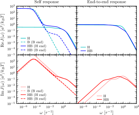
Figure S.1: The panels show the handle-bead (HB) response functions, taken from Fig. 2 in the main text, along with functions for the handle (H) and bead (B) separately. The self and end-to-end response functions are in the left and right columns respectively, with real parts in the top row and imaginary parts in the bottom row.

As described in the main text, the HB response functions reflect the contributions of their handle and bead components. To elucidate this, we plot in Fig. S.1 the HB functions from Fig. 2, together with the individual H and B functions. As expected, the HB self response at the H end is very similar to the individual H response, and at the B end it is close to the individual B response. For the HB end-to-end function, only comparison with the handle component is possible (since the bead end-to-end response is zero). Again the two functions are similar, but clearly adding the bead onto the handle perturbs its end-to-end response, shifting it to lower frequencies and changing its shape. The way in which the components contribute to the response of the total object is not merely additive, and requires the convolution rules in order to be to accurately predicted.

VI Dynamic deconvolution of a double-well protein

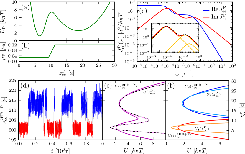
Figure S.2: Analysis of an optical tweezer system with the protein modeled using a double-well potential. (a) The protein potential $U_{\text{P}}$ as a function of end-to-end distance $z^{\text{P}}_{\text{ee}}$, from Eq. (S.29). The potential as shown is tilted by the external stretching force $F=3$ $k_{B}T/a$. (b) The protein mobility profile $\mu_{\text{P}}(z^{\text{P}}_{\text{ee}})$. (c) Formal linear response result for $J^{\text{P}}_{\text{ee}}(\omega)$ based on a numerical Fokker-Planck solution using the full profiles in (a) and (b). Inset: $\text{Im}\,J^{\text{P}}_{\text{ee}}(\omega)$ (red curve), with analytical estimates for the three contributions to the protein response (orange). The sum of these analytical estimates is shown as a dashed black curve. (d) Fragment of time series for $z^{\text{2HB+P}}_{\text{ee}}$, with the portions assigned to either the folded or unfolded wells colored red and blue respectively. The remainder is shaded gray. (e) The full system free energy profile $U(z^{\text{2HB+P}}_{\text{ee}})$ calculated from the simulation (dark purple), together with the protein-only result $U(z^{\text{P}}_{\text{ee}})$ (light purple) obtained by static deconvolution using the 2HB distribution in Fig. 2(b) of the main text. This agrees with the original theoretical form, Eq. (S.29), shown as a dashed line. (f) For the time series in each well, the corresponding full system potential $U_{i}(z^{\text{2HB+P}}_{\text{ee}})$ (blue/red lines) and the deconvolved result $U_{i}(z^{\text{P}}_{\text{ee}})$ (cyan/orange lines), $i=1,2$.

Instead of the single-well protein of the main text, we start with a double-well potential $U_{\text{P}}(z^{\text{P}}_{\text{ee}})$ shown in Fig. S.2(a). This potential arises from the force:

$$F_{\text{P}}(z)=\begin{cases}-k_{1}(z-z_{1})&z\leq\frac{k_{m}z_{m}+k_{1}z_{1}}{k_{1}+k_{m}}\\ k_{m}(z-z_{m})&\frac{k_{m}z_{m}+k_{1}z_{1}}{k_{1}+k_{m}}<z\leq\frac{k_{m}z_{m}+k_{2}z_{2}}{k_{2}+k_{m}}\\ -k_{2}(z-z_{2})&\frac{k_{m}z_{m}+k_{2}z_{2}}{k_{2}+k_{m}}<z\end{cases},$$ (S.29)

where the parameters $k_{1}=2\>k_{B}T/a^{2}$, $k_{m}=1.5\>k_{B}T/a^{2}$, $k_{2}=0.15\>k_{B}T/a^{2}$, $z_{1}=5a$, $z_{m}=12.3a$, $z_{2}=-1.3a$. The energy profile plotted in Fig. S.2(a) has been additionally tilted by a contribution $Fz$ representing the equilibrium stretching at constant force $F=3\>k_{B}T/a$. To mimic the effects of internal friction on the protein dynamics, we allow for a coordinate-dependent mobility $\mu_{\text{P}}(z^{\text{P}}_{\text{ee}})$, which is plotted in Fig. S.2(b). In the left well $\mu_{\text{P}}=0.03\>\mu_{0}$ (folded state), while in the right well we have a higher value $\mu_{\text{P}}=0.12\>\mu_{0}$ (unfolded state), with a linear transition of width $2a$ around the energy barrier. For real proteins, larger internal friction in the folded state may occur due to a greater proportion of intact native bonds compared to unfolded configurations.

Formally, the protein end-to-end response $J^{\text{P}}_{\text{ee}}(\omega)$ may be derived for this double-well potential using a numerical solution of the corresponding Fokker-Planck equation, based on the method of Bicout and Szabo Bicout98 . The numerical procedure consists of the following steps. We discretize our potential $U_{\text{P}}(z_{i})$ over $M$ values $z_{i}$, $i=1,\ldots,M$, in some range $z_{\text{min}}$ to $z_{\text{max}}$. The bin size $d=(z_{\text{max}}-z_{\text{min}})/M$. Define local equilibrium probabilities $p_{i}=\exp(-U_{\text{P}}(z_{i})/k_{B}T)/Z$, where $Z=\sum_{i}\exp(-U_{\text{P}}(z_{i})/k_{B}T)$. Transition frequencies $w(i|j)$ of going from bin $i$ to bin $j$ are given by:

$$w(i|j)=k_{B}T\frac{\mu_{\text{P}}(z_{i})+\mu_{\text{P}}(z_{j})}{2d^{2}}\exp\left(-\frac{\beta(U_{\text{P}}(z_{i})-U_{\text{P}}(z_{j}))}{2}\right).$$ (S.30)

Reflective boundary conditions at the ends of our range are imposed by defining $w(0|1)=w(1|0)=w(M|M+1)=w(M+1|M)=0$. The $M\times M$ symmetric rate matrix $R$ has the nonzero elements:

$$R_{i,i}=-w(i+1|i)-w(i-1|i),\qquad R_{i,i\pm 1}=R_{i\pm 1,i}=\sqrt{w(i\pm 1|i)w(i|i\pm 1)}.$$ (S.31)

The eigenvalues and eigenvectors of this matrix satisfy an equation of the form: $R\mathbf{v}_{\alpha}=-\Lambda_{\alpha}\mathbf{v}_{\alpha}$, where the index $\alpha=0,\ldots,M-1$ and we arrange the eigenvalues in increasing order. With reflective boundary conditions at either end, the smallest eigenvalue is always $\Lambda_{0}=0$. The correlation function $C^{\text{P}}_{\text{ee}}(t)=\langle z_{\text{ee}}^{\text{P}}(t)z_{\text{ee}}^{\text{P}}(0)\rangle$ for the protein is then given by $C^{\text{P}}_{\text{ee}}(t)=\sum_{\alpha=1}^{M-1}C_{\alpha}e^{-\Lambda_{\alpha}t}$, where the coefficients $C_{\alpha}$ are:

$$C_{\alpha}=\sum_{i=1}^{M}\left(\sqrt{p_{i}}z_{i}v_{\alpha i}\right)^{2}.$$ (S.32)

Here $v_{\alpha i}$ is the $i$th component of the eigenvector $\mathbf{v}_{\alpha}$. Finally, from the fluctuation-dissipation theorem, the time-domain response function $J^{\text{P}}_{\text{ee}}(t)$ is related to $C^{\text{P}}_{\text{ee}}(t)$ through $J^{\text{P}}_{\text{ee}}(t)=-\beta dC^{\text{P}}_{\text{ee}}(t)/dt$. After a Fourier transform, we get the response function:

$$J^{\text{P}}_{\text{ee}}(\omega)=\sum_{\alpha=1}^{M-1}\frac{\beta C_{\alpha}\Lambda_{\alpha}}{\Lambda_{\alpha}-i\omega},$$ (S.33)

where all the parameters $\{C_{\alpha},\Lambda_{\alpha}\}$ are known numerically.

This response function is shown in Fig. S.2(c). Its structure can actually be decomposed into three contributions, as shown in the inset: two correspond to fluctuations of the protein about the local minima; the third, at lower frequencies, corresponds to transitions between the wells. The orange curves in the inset are simple analytical predictions for these contributions: the two intrawell peaks at higher frequencies are just single Lorentzians with the appropriate values of $k$ and $\mu_{\text{P}}$ for each well, and the interwell transition peak is a based on a discrete two-state description Wio99 . Though approximate, the analytical sum (dashed line) captures well the exact numerical result (red line).

However if we go beyond this and try to naively apply the convolution theory on the $J^{\text{P}}_{\text{ee}}(\omega)$ of Fig. S.2(c), the results for the total system will deviate from the actual behavior as seen in simulations. This is not surprising, since the (large amplitude, low frequency) transitions between wells are a fundamentally nonlinear process, and thus violate the linear response assumption on which our theory is based. To correctly apply our analysis in this situation, we should focus on the linear response of the system within each state, where the protein fluctuates about the local minimum: in essence, we break the problem into two single-well systems.

To implement this approach, we need to extract “single-well” time series from the full simulation data, a portion of which is shown in Fig. S.2(d). Since what we measure is the end-to-end behavior of the total system, we choose the separation line between wells to lie at the barrier position in the full system free energy profile $U(z^{\text{2HB+P}}_{\text{ee}})=-k_{B}T\log{\cal P}(z^{\text{2HB+P}}_{\text{ee}})$ [Fig. S.2(e)]. Segments of the time series falling on either side of the separation line will be assigned to well 1 (folded) or well 2 (unfolded), with the following exceptions: points that are within a certain time window $\pm\delta t$ of a transition (i.e. a crossing of the separation line) are excluded. Setting $\delta t$ to $10^{6}\tau$, longer than the relaxation times within the wells, this exclusion ensures that the resulting single-well time series are not significantly perturbed by memory effects from the transitions. Note that times both before and after each transition are excluded in order to preserve the time-reversal symmetry of the equilibrium time series. For the time series in Fig. S.2(d), the parts assigned to well 1 and 2 are colored red and blue respectively, with the remainder shaded gray. The same method can be generalized to a more complicated free energy landscape, for example in a protein with intermediate states, to get a single-well time series corresponding to every state.

The end-to-end distributions from the single-well series yield corresponding energy profiles $U_{1}(z^{\text{2HB+P}}_{\text{ee}})$ and $U_{2}(z^{\text{2HB+P}}_{\text{ee}})$, shown in Fig. S.2(f). After static deconvolution with the double-HB distribution from Fig. 2(b), we get profiles in terms of the protein end-to-end distance: $U_{1}(z^{\text{P}}_{\text{ee}})$ and $U_{2}(z^{\text{P}}_{\text{ee}})$. Near the minima these are identical to the original $U_{\text{P}}$, but have anharmonic corrections as they approach infinity at the separation line. The dynamic deconvolution analysis for each well is analogous to the simple parabolic case described in the main text, except instead of the single Lorentzian we will use the corrected $J^{\text{P}}_{\text{ee}}$ based on the Fokker-Planck numerical solution with $U_{1}(z^{\text{P}}_{\text{ee}})$ and $U_{2}(z^{\text{P}}_{\text{ee}})$. This yields a generalized form in each well: $J^{\text{P}}_{\text{ee}}(\omega)=\sum_{\alpha}\frac{\beta C_{\alpha}\Lambda_{\alpha}}{\Lambda_{\alpha}-i\omega}$, with the multiple Lorentzians accounting for the anharmonic corrections. For the parabolic case, $C_{1}=k_{B}T/k$, $\Lambda_{1}=\mu_{\text{P}}k$, and there were no other terms. Given a $\mu_{\text{P}}$ for the well, the parameters $\{C_{\alpha},\Lambda_{\alpha}\}$ are known from the Fokker-Planck solution. (In fact only the $\Lambda_{\alpha}$ depend on the diffusion constant; note that $J^{\text{P}}_{\text{ee}}(0)=\sum_{\alpha}\beta C_{\alpha}=\beta\langle(z^{\text{P}}_{\text{ee}})^{2}\rangle$ is an equilibrium average, so the $C_{\alpha}$ must be independent of $\mu_{\text{P}}$).

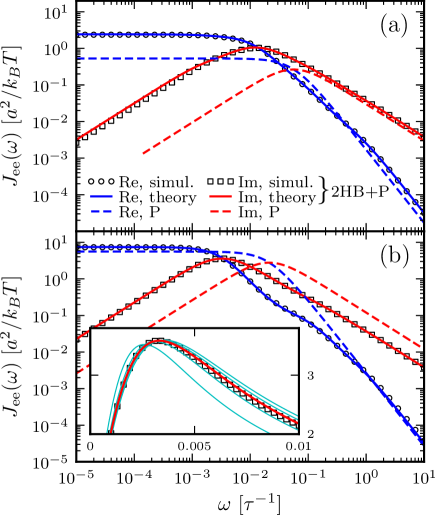
Figure S.3: Analogous to Fig. 3 in the main text, showing the accuracy of the theoretical prediction of the total system end-to-end response $J^{\text{2HB+P}}_{\text{ee}}(\omega)$ using the double-well protein model. The (a) folded and (b) unfolded states are analyzed separately, with the simulation results plotted as symbols and the theory as solid lines. The latter uses the true values of $\mu_{\text{P}}=0.03$ $\mu_{0}$ in the folded state and $\mu_{\text{P}}=0.12$ $\mu_{0}$ in the unfolded state. Blue/red results denote the Re/Im parts respectively. For comparison, the protein response $J^{\text{P}}_{\text{ee}}(\omega)$ (dashed line) is also shown for each well, based on the local Fokker-Planck numerical solution. Inset to (b): for the unfolded state, a zoomed-in section of the $\text{Im}\,J^{\text{2HB+P}}_{\text{ee}}(\omega)$ peak, with simulation (symbols) and theoretical (red curve) results. The cyan curves are theoretical results with $\mu_{\text{P}}$ different from the true value: from left to right, $\mu_{\text{P}}=0.04$, $0.08$, $0.016$, $0.24$ $\mu_{0}$.

As in the single-well example, applying the convolution of $J^{\text{P}}_{\text{ee}}$ with the HB response functions, and comparing with the simulation results, shows excellent agreement [Fig. S.3]. Here the theoretical curves (red lines) for each well are based on setting $\mu_{\text{P}}$ to the values at the minima. For the unfolded state, the inset in Fig. S.3 shows how this theoretical result shifts if $\mu_{\text{P}}$ is displaced from the true value of $0.12\>\mu_{0}$. The sensitivity of the theoretical fitting allows one to numerically extract good estimates for $\mu_{\text{P}}$ in each well: $\mu_{\text{P}}=0.033\>\mu_{0}$ (folded) and $\mu_{\text{P}}=0.111\>\mu_{0}$ (unfolded), where the exact values are $0.03\>\mu_{0}$ and $0.12\>\mu_{0}$ respectively. Given the complications associated with excluding interwell hopping (and the nonconstant diffusion profile across the barrier), it is remarkable that we can still fit to within $\approx 10\%$ of the true values. If one was interested in getting just an estimate of $\mu_{\text{P}}$ in each well, without necessarily getting a perfect fit for the total system response, the anharmonic corrections could be ignored and the single Lorentzian form used instead of the exact $J^{\text{P}}_{\text{ee}}$ in the fitting. The resulting values for $\mu_{\text{P}}$ have a comparable accuracy.

VII Accounting for experimental limitations: noise, drift, and finite time resolution

Practical implementation of the deconvolution theory on experimental time series must take into account possible errors due to instrumental limitations. We will focus on the optical tweezer apparatus in particular, since this is the example analyzed in the main text. However the techniques discussed below are applicable in a generic experimental setup. For optical tweezers, effects like drift and noise which enter into the measured output are typically divided into “experimental” and “Brownian” categories Moffitt08 : the former arises from the instrumental components, while the latter is related to thermal fluctuations of the beads and the objects under study. Equilibrium Brownian noise is completely captured within the deconvolution theory: the linear response formalism provides a quantitative prediction of exactly how each thermally fluctuating part of the system will contribute to the total signal. We will thus concentrate on experimental effects, and outline how they enter into the theoretical deconvolution procedure.

For a perfect instrument, the raw data collected by the experimentalist would be a “true” time series $z_{\alpha}(t_{i})$ at discrete time steps $t_{i}$, where $\alpha$ refers to either one of the bead positions ($\alpha=\text{B,L}$ or B,R), or the bead-bead separation ($\alpha=\text{ee}$). The sampling time $t_{\text{s}}\equiv t_{i+1}-t_{i}$ is the time resolution of the apparatus. In any realistic scenario, the actual measured time series is $\tilde{z}_{\alpha}(t_{i})=z_{\alpha}(t_{i})+\eta_{\alpha}(t_{i})$, where $\eta_{\alpha}(t_{i})$ is an extraneous signal due to the instrument. We will consider two possible contributions to $\eta_{\alpha}(t)$: a) white noise, or any high-frequency random signal that is uncorrelated at time scales above $t_{\text{s}}$; b) a low-frequency signal related to instrumental drift over an extended measurement period. The latter can result from environmental factors like slow temperature changes and air currents that affect the laser beam position. As a side note, one of the advantages of the dual-trap setup illustrated in the text is a dramatic reduction of such drift effects, relative to earlier designs involving a single trap and biomolecules tethered to a surface Moffitt08 . Whereas the beam position of a single trap will move over time relative to the surface, the dual traps are created from a single laser, and hence any overall drift in the beam position will not affect the trap separation. (Though smaller issues may exist, like the effective mobility of the beads shifting as the distance from the sample chamber surface varies.) In any case, the low drift of the dual-trap setup allows for long, reliable data collection periods (i.e. on the order of a minute in the leucine zipper study of Ref. Gebhardt10 ).

The final experimental effect we will describe in this section relates to the time resolution: the sampling period $t_{\text{s}}$ cannot be made smaller than a certain value, dependent on the instrumentation. Not only is the frequency of data collection limited, but because the electronics have a finite response time, there will also effectively be some kind of averaging of the true signal across the $t_{\text{s}}$ time window between measurements. Both of these effects can be incorporated into the deconvolution analysis, and we will illustrate this concretely through the toy model protein simulation data discussed in the main text. These simulations had data collection at intervals of $0.3\tau=1.2$ ns, in order to clearly illustrate that the theory is valid over a wide frequency regime encompassing the characteristic fluctuations of all the system components. However we can mimic the experimental apparatus by resampling and averaging the data over windows of size $t_{\text{s}}=0.01$ ms (the resolution of the Gebhardt et. al. Gebhardt10 setup). The deconvolution procedure works for the reduced frequency range (up to $\omega_{s}=t_{\text{s}}^{-1}$), and the main quantity of interest (the protein diffusivity) can still be extracted with good accuracy. The reason for this is that the protein characteristic frequency in our example (after being slowed down by the handles and beads) falls under the cutoff $\omega_{s}$. In general, any component fluctuation modes with frequencies $\omega\lesssim\omega_{s}$ can be deconvolved using the theory, even though we lack information about higher frequency modes above the cutoff. Though we may not be able to directly observe the modes of certain objects—like the short DNA handles whose characteristic frequencies are $\sim{\cal O}(1\>\text{ns})$—this does not impede us from exploiting the full physical content of the time series in the frequency range below $\omega_{s}$.

We begin our detailed discussion with the white noise and drift effects that contribute to $\eta_{\alpha}(t)$.

VII.1 White noise and drift

Consider the situation where our time series is contaminated by a Gaussian white noise signal $\eta_{\alpha}(t_{i})$, with zero mean and correlation $\langle\eta_{\alpha}(t_{i})\eta_{\alpha}(t_{j})\rangle=\gamma\delta_{ij}$. We will also assume that the white noise is to a good approximation not correlated with the true component signal: $\langle\eta_{\alpha}(t_{i})z_{\alpha}(t_{j})\rangle=0$, $\forall i,j$. From the measured time series $\tilde{z}_{\alpha}(t_{i})=z_{\alpha}(t_{i})+\eta_{\alpha}(t_{i})$ the main quantity which enters the deconvolution theory is the MSD function:

$$\begin{split}\tilde{\Delta}_{\alpha}(t_{i})=\langle(\tilde{z}_{\alpha}(t_{i})-\tilde{z}_{\alpha}(0))^{2}\rangle&=\langle({z}_{\alpha}(t_{i})-{z}_{\alpha}(0))^{2}\rangle+\langle(\eta_{\alpha}(t_{i})-\eta_{\alpha}(0))^{2}\rangle\\ &=\Delta_{\alpha}(t_{i})+2\gamma,\end{split}$$ (S.34)

where $\Delta_{\alpha}(t_{i})$ is the true MSD value. Thus the white noise induces a uniform upward shift of the MSD, which is irrelevant to the theoretical analysis, since we are interested only in the MSD slope, which determines the linear response function $\tilde{J}_{\alpha}(t)=(\beta/2)d\tilde{\Delta}_{\alpha}(t)/dt=J_{\alpha}(t)$. However this assumes that we can collect an infinite time series, reducing the statistical uncertainty of our expectation values to zero. In reality, our sampling is carried out only $N$ times, over a finite time interval $T_{\text{s}}=Nt_{s}$. Our calculated $\tilde{\Delta}_{\alpha}(t_{i})$ for this time interval will differ from the $T_{\text{s}}\to\infty$ result by some random amount characterized by a standard deviation $\sigma(\tilde{\Delta}_{\alpha}(t_{i}))$. The standard error analysis for correlation functions Zwanzig69 ; Frenkel (which assumes Gaussian-distributed fluctuations) yields an approximate magnitude for $\sigma(\tilde{\Delta}_{\alpha}(t_{i}))$, up to lowest order in $\gamma$:

$$\sigma(\tilde{\Delta}_{\alpha}(t_{i}))=\sqrt{A\frac{\tau_{\alpha}\Gamma^{2}_{\alpha}}{Nt_{\text{s}}}\left[1+\frac{16t_{\text{s}}}{A\tau_{\alpha}}\frac{\gamma}{\Gamma_{\alpha}}+{\cal O}\left(\frac{\gamma^{2}}{\Gamma_{\alpha}^{2}}\right)\right]}.$$ (S.35)

Here $A\sim{\cal O}(1)$ is a numerical prefactor (which may depend on $t_{i}$), $\Gamma_{\alpha}=\langle z_{\alpha}^{2}\rangle-\langle z_{\alpha}\rangle^{2}$, and $\tau_{\alpha}=2\Gamma_{\alpha}^{-2}\int_{0}^{\infty}dt\,(\langle z_{\alpha}(t)z_{\alpha}(0)\rangle-\langle z_{\alpha}\rangle^{2})^{2}$ is an effective correlation time. Since $\Delta_{\alpha}(t)$ can be modeled as a sum of terms exponentially converging toward the long-time limit $\Delta_{\alpha}(\infty)=2\Gamma_{\alpha}$, the value of $\tau_{\alpha}$ is on the order of the longest decay time. Eq. (S.35) allows us to see how to correct the effects of white noise: if in the absence of noise ($\gamma=0$) we could achieve a certain statistical uncertainty by taking $N_{0}$ steps, the same uncertainty could be obtained in the presence of white noise by taking a larger number of steps, $N\approx N_{0}(1+16t_{\text{s}}\gamma/A\tau_{\alpha}\Gamma_{\alpha})$.

Generally the larger the correlation time $\tau_{\alpha}$ for the specific MSD of interest, the longer the sampling time necessary to achieve a certain level of precision (i.e. a self MSD, involving the motion of the individual trapped beads, will typically have a slower relaxation time than an end-to-end MSD). If the largest $\tau_{\alpha}$ is $\sim 0.1$ ms (an upper bound estimate for the dual-trap setup discussed in the main text), $t_{\text{s}}=0.01$ ms, and $\Gamma_{\alpha}\sim 10$ nm² is the characteristic scale of the MSD function, then a 1% precision, $\sigma(\tilde{\Delta}_{\alpha}(t_{i}))/\Gamma_{\alpha}=0.01$, requires a sampling time of $T_{\text{s}}\sim 1$ s (with no white noise). The same precision with a noise strength of $\gamma=1$ nm² would need $\sim 16\%$ more sampling time.

In contrast to the high frequency noise modeled above, imagine that we have a low frequency contamination induced by slow drift: $\eta(t_{i})=t_{i}/t_{\text{d}}+\eta_{0}$ for some constants $t_{\text{d}}$ and $\eta_{0}$. The measured MSD becomes:

$$\begin{split}\tilde{\Delta}_{\alpha}(t_{i})=\langle(\tilde{z}_{\alpha}(t_{i})-\tilde{z}_{\alpha}(0))^{2}\rangle&=\langle({z}_{\alpha}(t_{i})-{z}_{\alpha}(0))^{2}\rangle+\langle(\eta_{\alpha}(t_{i})-\eta_{\alpha}(0))^{2}\rangle\\ &=\Delta_{\alpha}(t_{i})+(t_{i}/t_{\text{d}})^{2}.\end{split}$$ (S.36)

Thus instead of reaching a plateau at large times, the MSD continues to increase $\propto t^{2}$. If any deviation of this kind is observed in the experimental time series, the simplest solution is to fit the long-time MSD, extract the functional form (i.e. the slope $1/t_{\text{d}}^{2}$), and subtract the drift contribution from $\tilde{\Delta}_{\alpha}(t_{i})$ to recover $\Delta_{\alpha}(t_{i})$. Alternatively, since the drift time scale is typically larger than any characteristic relaxation time in the system, $t_{\text{d}}\gg\tau_{\alpha}$, one could collect data from many short runs of length $T_{\text{s}}$, where $\tau_{\alpha}\ll T_{\text{s}}\ll t_{\text{d}}$.

VII.2 Limited time resolution

In addition to the possibilities of noise and drift modifying the signal, we have to consider that the measuring apparatus will have some finite time resolution $t_{\text{s}}$, defined as the interval between consecutive recordings of the data. The measured value, $\tilde{z}_{\alpha}(t_{i})$, even in the absence of noise contributions $\eta(t_{i})$, only approximately corresponds to the instantaneous true value $z_{\alpha}(t_{i})$. Because of the finite response time of the equipment, it is more realistic to model $\tilde{z}_{\alpha}(t_{i})$ as some weighted average from the previous $t_{\text{s}}$ interval:

$$\tilde{z}_{\alpha}(t_{i})=W^{-1}\int_{-t_{\text{s}}}^{0}ds\,z_{\alpha}(t_{i}+s)w(s),\qquad W=\int_{-t_{\text{s}}}^{0}ds\,w(s),$$ (S.37)

for some weighting function $w(s)$. In the present discussion we will ignore any contributions from white noise and drift in the time-averaged signal, since these can be corrected for in the same manner as described above. The measured autocorrelation function $\tilde{R}_{\alpha}(t_{i}-t_{j})=\langle\tilde{z}_{\alpha}(t_{i})\tilde{z}_{\alpha}(t_{j})\rangle$ between two time points $t_{i}$ and $t_{j}$ is related to the true function $R_{\alpha}(t_{i}-t_{j})=\langle z_{\alpha}(t_{i})z_{\alpha}(t_{j})\rangle$ as follows:

$$\begin{split}\tilde{R}_{\alpha}(t_{i}-t_{j})&=W^{-2}\int_{-t_{\text{s}}}^{0}ds\int_{-t_{\text{s}}}^{0}ds^{\prime}\,R_{\alpha}(t_{i}+s-t_{j}-s^{\prime})w(s)w(s^{\prime})\\ &\equiv\int_{-\infty}^{\infty}dt^{\prime}\,B(t^{\prime})R_{\alpha}(t_{i}-t_{j}-t^{\prime}),\end{split}$$ (S.38)

where we introduce the combined weighting function:

$$B(t)=\frac{1}{2W^{2}}\Theta(t+t_{\text{s}})\Theta(-t+t_{\text{s}})\int_{|t|-2t_{\text{s}}}^{-|t|}dt^{\prime}\,w\left(\frac{t^{\prime}-t}{2}\right)w\left(\frac{t^{\prime}+t}{2}\right).$$ (S.39)

While the precise weighting function may vary depending on the apparatus, a reasonable approximation is that $w(s)\approx 1$, or that the signal is directly an average over the $t_{\text{s}}$ interval. Plugging this into Eq. (S.39), with $W=t_{\text{s}}$, we find:

$$B(t)=\Theta(t+t_{\text{s}})\Theta(-t+t_{\text{s}})\frac{1}{t_{\text{s}}}\left(1-\frac{|t|}{t_{\text{s}}}\right).$$ (S.40)

The autocorrelation $R_{\alpha}(t)$ enters the deconvolution analysis through the MSD $\Delta_{\alpha}(t)=2(R_{\alpha}(0)-R_{\alpha}(t))$, and its derivative $J_{\alpha}(t)=(\beta/2)d\Delta_{\alpha}(t)/dt=-\beta dR_{\alpha}(t)/dt$. If $R_{\alpha}(t)$ is expressed as a sum of decaying exponentials, $R_{\alpha}(t)=\sum_{i}A_{i}\exp(-\Lambda_{i}t)$, then this corresponds to $J_{\alpha}(t)=\sum_{i}C_{i}\exp(-\Lambda_{i}t)$ with the coefficients $C_{i}=\beta\Lambda_{i}A_{i}$. Assuming this underlying exponential form, the relationship between the measured and actual $R_{\alpha}(t)$ can be calculated using Eqs. (S.38) and (S.40):

$$\tilde{R}_{\alpha}(t)=\int_{-\infty}^{\infty}dt^{\prime}\,B(t^{\prime})R_{\alpha}(t-t^{\prime})=\sum_{i}\frac{2(\cosh(\Lambda_{i}t_{\text{s}})-1)}{\Lambda_{i}^{2}t_{\text{s}}^{2}}A_{i}e^{-\Lambda_{i}t}\equiv\sum_{i}\tilde{A}_{i}e^{-\Lambda_{i}t},\qquad t\geq t_{\text{s}}.$$ (S.41)

Thus the only modification is in the coefficient of each exponential term, $\tilde{A}_{i}=p(\Lambda_{i}t_{s})A_{i}$, which gets a prefactor $p(x)=2(\cosh(x)-1)/x^{2}>1$ dependent on $x=\Lambda_{i}t_{\text{s}}$. The restriction to times $t\geq t_{\text{s}}$ comes from the fact that $\tilde{R}_{\alpha}(t)$ cannot be measured for times smaller than the experimental resolution. The prefactor $p(x)$ is only appreciably larger than 1 for relaxation times $\Lambda_{i}^{-1}$ comparable to or smaller than $t_{\text{s}}$. However, even for $\Lambda_{i}^{-1}=t_{\text{s}}$, which is roughly the smallest relaxation time we can realistically fit from the measured data, $p(1)=1.09$, so the averaging effect is modest.

Thus when we fit a sum of exponentials to the $J_{\alpha}(t)$ functions derived from the experimental time series, we are effectively calculating $\tilde{C}_{i}=\beta\Lambda_{i}\tilde{A}_{i}$ and $\Lambda_{i}$. To recover the actual $C_{i}$, we just divide out the prefactor: $C_{i}=\tilde{C}_{i}/p(\Lambda_{i}t_{\text{s}})$. In this way we correct for the distortion due to time averaging.

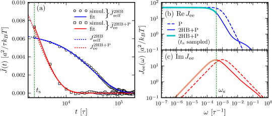
Figure S.4: (a) Time-domain response functions $\tilde{J}_{\text{self}}^{\text{2HB}}(t)$ (circles) and $\tilde{J}_{\text{ee}}^{\text{2HB+P}}(t)$ (squares) calculated from coarse-grained simulation time series of the 2HB and 2HB+P systems respectively. The coarse-graining involved averaging over intervals of $t_{\text{s}}=2500\tau=0.01$ ms, and using the time series of mean values. The solid lines are the results of single-exponential fitting to the data. The original fit results based on the fine-grained time series, ${J}_{\text{self}}^{\text{2HB}}(t)$ and ${J}_{\text{ee}}^{\text{2HB+P}}(t)$, are shown as dashed lines for comparison. (b,c) The thin dashed and solid lines are the theoretical predictions for the Fourier-domain end-to-end responses $J^{\text{P}}_{\text{ee}}(\omega)$ and $J^{\text{2HB+P}}_{\text{ee}}(\omega)$ respectively; panel (b) shows the real part, panel (c) the imaginary part. These are taken from Fig. 3 in the main text. The thick solid lines are Re and Im $J^{\text{2HB+P}}_{\text{ee}}(\omega)$ as determined from the time-domain best-fit in panel (a), after correcting for the averaging effect. The vertical dotted line marks the frequency cutoff $\omega_{\text{s}}=t_{\text{s}}^{-1}$ for the coarse-grained data.

To illustrate the effects of the experimental time resolution, and how the above corrections would work in practice, we will redo the deconvolution analysis for the toy protein example described in the main text. However, instead of using the original simulation time series, whose data collection interval was 1.2 ns, we will average the data over windows of width $t_{\text{s}}=2500\tau=0.01$ ms, and use the time series of these mean values, spaced at intervals of $t_{\text{s}}$ (with a total sampling time $T_{\text{s}}\approx 0.5$ s). We thus roughly mimic the apparatus of Ref. Gebhardt10 . Fig. S.4(a) shows time-domain response functions derived from the coarse-grained data: $\tilde{J}_{\text{self}}^{\text{2HB}}(t)$, from the first deconvolution step, involving the beads and handles alone; $\tilde{J}_{\text{ee}}^{\text{2HB+P}}(t)$, from the second step, where the toy protein is included in the system. The fits, drawn as solid lines, involve only single exponentials, since these are sufficient to capture the behaviors in the restricted time range $t\geq t_{\text{s}}$. From the Fourier transform of the fit results for $\tilde{J}_{\text{ee}}^{\text{2HB+P}}(t)$ (with the $\tilde{C}_{i}\to C_{i}$ correction) we can get the true frequency space linear response of the 2HB+P system, $J_{\text{ee}}^{\text{2HB+P}}(\omega)$. The real and imaginary parts of this response are drawn as thick solid lines in Fig. S.4(b) and (c) respectively. As expected, we can calculate this response only up to the cutoff frequency $\omega_{\text{s}}=t_{\text{s}}^{-1}=4\times 10^{-4}\tau^{-1}$ of the measuring equipment. However, it coincides very well with the theoretical prediction (thin solid lines, taken from Fig. 3 of the main text).

Even though we are limited to the range $\omega<\omega_{\text{s}}$, the convolution rules still work: a relation like Eq. [3] in the main text is valid at all individual values of $\omega$. Though we see only a restricted portion of the total system end-to-end response $J_{\text{ee}}^{\text{2HB+P}}(\omega)$, it does exhibit non-trivial structure for $\omega<\omega_{\text{s}}$, i.e. the downturn in the real part and leveling off of the imaginary part at $\omega\gtrsim 10^{-4}\tau^{-1}$. Deconvolution allows us to extract the physical content of this structure: when numerical fitting is carried out over the range $\omega<\omega_{\text{s}}$, we find toy protein parameters: $\mu_{\text{P}}=0.0472\pm 0.005\>\mu_{0}$, $k_{\text{P}}=0.0201\pm 0.0001\>k_{B}T/a^{2}$, within 6% of the exact values ($0.05\>\mu_{0}$ and $0.02\>k_{B}T/a^{2}$).

What is the main reason behind the relative success of the fitting in extracting the protein parameters, despite the limited time resolution? Fig. S.4(b,c) also shows the theoretical response $J^{\text{P}}_{\text{ee}}(\omega)$ for the protein alone, which has a characteristic frequency $\mu_{\text{P}}k_{\text{P}}=10^{-3}\tau^{-1}$, above the equipment cutoff $\omega_{\text{s}}=4\times 10^{-4}\tau^{-1}$. (Graphically, the peak in $J^{\text{P}}_{\text{ee}}(\omega)$ falls to the right of the vertical dotted line marking $\omega_{\text{s}}$.) However, the protein dynamics is modified by the presence of the handles and beads in the experimental system, in a manner quantitatively described by our convolution theory. As a result, the characteristic frequency of the protein within the experimental apparatus (i.e. the peak position in the imaginary part) is shifted to $\omega=3.6\times 10^{-4}\tau^{-1}$, just within the cutoff. Hence we are able to fit for the protein properties. The relative accuracy of the fitting is notable, since we are essentially at the very limit of resolvability. This example illustrates a general principle: whatever dynamical features a protein (or any other component) exhibits at $\omega<\omega_{\text{s}}$ within the full experimental setup, our deconvolution theory should be able to extract. For this purpose, knowledge of the system behavior for $\omega>\omega_{\text{s}}$ is not necessary. In the current case, the theoretical 2HB+P end-to-end response has a contribution at $\omega\gtrsim 10^{-2}\tau^{-1}$ due to the DNA handle fluctuation modes, i.e. the shoulder seen in Fig. S.4(b,c). These modes are experimentally inaccessible at our time resolution $t_{\text{s}}$, so the coarse-grained time series reveals nothing about their properties. However, this does not stop us from applying the theory at $\omega<\omega_{\text{s}}$.

References

- (1) Kim S, Karrila SJ (1991) Microhydrodynamics: Principles and Selected Applications (Dover Publications, Mineola).
- (2) Blake JR (1971) Image system for a stokeslet in a no-slip boundary. Proc. Camb. Philos. Soc-math. Ph. 70:303–310.
- (3) Doi M, Edwards SF (1988) The Theory of Polymer Dynamics (Oxford University Press, USA).
- (4) Coffey WT, Kalmykov YP, Waldron JT (2004) The Langevin Equation, 2nd Ed. (World Scientific, New Jersey).
- (5) Szabo A (1980) Theory of polarized fluorescent emission in uniaxial liquid-crystals. J. Chem. Phys. 72:4620–4626.
- (6) Granek R (1997) From semi-flexible polymers to membranes: Anomalous diffusion and reptation. J. Phys. II (France) 7:1761–1788.
- (7) Harnau L, Winkler RG, Reineker P (1996) Dynamic structure factor of semiflexible macromolecules in dilute solution. J. Chem. Phys. 104:6355–6368.
- (8) Hinczewski M, Schlagberger X, Rubinstein M, Krichevsky O, Netz RR (2009) End-monomer Dynamics in Semiflexible polymers. Macromol. 42:860–875.
- (9) Marko JF, Siggia ED (1995) Stretching DNA. Macromol. 28:8759–8770.
- (10) Meiners JC, Quake SR (2000) Femtonewton force spectroscopy of single extended dna molecules. Phys. Rev. Lett. 84:5014–5017.
- (11) Bicout DJ, Szabo A (1998) Electron transfer reaction dynamics in non-Debye solvents. J. Chem. Phys. 109:2325–2338.
- (12) Wio H, Bouzat S (1999) Stochastic resonance: The role of potential asymmetry and non gaussian noises. Braz. J. Phys. 29:136–143.
- (13) Moffitt JR, Chemla YR, Smith SB, Bustamante C (2008) Recent advances in optical tweezers. Annu. Rev. Biochem. 77:205–228.
- (14) Gebhardt JCM, Bornschlögl T, Rief M (2010) Full distance-resolved folding energy landscape of one single protein molecule. Proc. Natl. Acad. Sci. U. S. A. 107:2013–2018.
- (15) Zwanzig R, Ailawadi NK (1969) Statistical error due to finite time averaging in computer experiments. Phys. Rev. 182:280–283.
- (16) Frenkel D, Smit B (2001) Understanding Molecular Simulation, 2nd Ed.: From Algorithms to Applications (Academic Press, San Diego).