Controlling the pair momentum of the FFLO state in a 3D Fermi gas through a 1D periodic potential.

Abstract

The question whether a spin-imbalanced Fermi gas can accommodate the Fulde-Ferrell-Larkin-Ovchinnikov (FFLO) state has been the subject of intense study. This state, in which Cooper pairs obtain a nonzero momentum, has hitherto eluded experimental observation. Recently, we demonstrated that the FFLO state can be stabilized in a 3D Fermi gas, by adding a 1D periodic potential. Until now it was assumed that the FFLO wave vector always lies parallel to this periodic potential (FFLO-P). In this contribution we show that, surprisingly, the FFLO wave vector can also lie skewed with respect to the potential (FFLO-S). Starting from the partition sum, the saddle-point free energy of the system is derived within the path-integral formalism. Minimizing this free energy allows us to study the different competing ground states of the system. To qualitatively understand the underlying pairing mechanism, we visualize the Fermi surfaces of the spin up and spin down particles. From this visualization, we find that tilting the FFLO wave vector with respect to the direction of the periodic potential, can result in a larger overlap between the pairing bands of both spin species. This skewed FFLO state can provide an additional experimental signature for observing FFLO superfluidity in a 3D Fermi gas.

I Introduction

Over the last decade, immense progress has been made in the field of the physics of ultracold atoms. These systems provide a versatile tool for studying various quantum many-body phenomena 1 - Bloch review ; 2 - Greiner Q and A . One example of the major breakthroughs in this field is the realization of a molecular Bose-Einstein condensate (BEC) 3 - Greiner ; 4 - Zwierlein Moleculair BEC and the observation of pair formation near a Feshbach resonance 5 - Jochim ; 6 - Bourdel ; 7 - Partridge Moleculair BEC ; 8 - Regal ; 9 - Zwierlein fermion condensate near Feshbach Reonance in a strongly interacting Fermi gas. These experimental discoveries preluded the observation of superfluidity in a gas of ultracold fermions 10 - Zwierlein fermionic superfluidity . The advantage of using ultracold Fermi gases to study superfluidity is that they allow to explore a wide range of parameter space. This is due to the tunability of the system parameters, such as the interaction strength and the spin imbalance. The possibility of adapting the interaction strength through the use of a Feshbach resonance 11a - Feshbach resonantie has allowed to study superfluid pairing in the crossover from a Bardeen-Cooper-Schrieffer (BCS) state of weakly bound Cooper pairs to a BEC of tightly bound molecules 11b - BCS-BEC crossover . Furthermore, in a Fermi gas composed of a mixture of two hyperfine states (labeled ”spin up” and ”spin down”), the ratio between the number of atoms in these two different states can be controlled with great precision. This last achievement has provided a unique experimental tool to study the effect of population imbalance on superfluidity. The first theoretical contribution in this context was provided by Clogston and Chandrasekhar, who predicted that a first order transition from a superfluid to a normal interacting Fermi gas would occur at a critical polarization 12 - Clogston Chandrasekhar . This quantum phase transition was indeed observed experimentally 13 - Zwierlein imbalanced SF ; 14 - Partridge Hulet imbalanced SF , along with the fact that when the system is in the BCS superfluid state, the excess particles are expelled from this state, leading to phase separation.

The question that has emerged here is whether there exist other, exotic quantum many body states that allow polarized superfluidity. In 1964, a new state was introduced independently by Fulde and Ferrell 15 - Fulde Ferell and by Larkin and Ovchinnikov 16 - Larkin Ovchinnikov . They proposed that a spin-polarized superfluid can be formed by creating Cooper pairs with finite center-of-mass-momentum. In the last seven years, extensive theoretical research has been done on this exotic superfluid state 17 - FFLO artikels . In 1D and quasi-1D systems, the Fulde-Ferrell-Larkin-Ovchinnikov (FFLO) state is predicted to be stable 17b - FFLO 1D and quasi-1D , and recently the first indirect experimental evidence for FFLO in a 1D system has been found 17c-Hulet . In general, lower dimensionality favors the FFLO state because of Fermi surface nesting at the FFLO wave vector. For the case of a three dimensional (3D) Fermi gas, it was found that the FFLO state only occurs on a restricted area of the BCS-to-BEC-crossover phase diagram 18 - Hu Liu ; 19 - Sheehy Radzihovsky . Up till know, the FFLO state has eluded experimental observation in a 3D Fermi gas. As an attempt to pave the path towards its experimental discovery, the idea was proposed to enhance FFLO pairing by using a 3D periodic optical lattice 20 - Koponen ; 21 - Trivedi . Recently, we proposed to subject the 3D Fermi gas to a one dimensional (1D) periodic potential as an alternative to achieve this goal 22 - Devreese Klimin Tempere . The 1D potential introduces an asymmetry into the system, which results in an energetically preferred direction for the FFLO wave vector, thus lowering the energy of this state compared to the normal state and to the BCS state.

In our previous work, it was assumed that the FFLO wave vector lies parallel to the periodic potential, since this is the energetically preferred direction. In this paper we show that, contrary to this intuitive expectation, the wave vector of the FFLO state can also lie skewed with respect to the direction along which the periodic potential lies. To qualitatively understand this counterintuitive phenomenon, we present a visualization of the underlying pairing mechanism by plotting the Fermi surfaces of the spin up and spin down fermions. This will pinpoint the effect of the periodic potential on the FFLO pairing mechanism. Our paper is structured as follows. In section II we calculate the free energy of the system through the use of the path integral formalism 23 - Kleinert ; 24 - De Melo . By choosing an appropriate saddle point, we incorporate the possibility of the FFLO state in our description, where we allow the FFLO wave vector to lie in an arbitrary direction. In section III.1 we minimize the free energy and discuss the different competing ground states of the system. Subsequently, in section III.2 we construct the phase diagram as a function of the total and imbalance chemical potential and in section III.3 we visualize and discuss the changes in the pairing mechanism of the FFLO state due to the presence of the periodic potential. Finally in section IV we draw conclusions.

II Path integral treatment

The starting point of our analytic treatment is the partition sum of a 3D spin-imbalanced Fermi gas, written in path integral form in units $\hbar=2m=1$

$$\mathcal{Z} =\int\mathcal{D}\bar{\psi}\mathcal{D}\psi~{}\exp\left(-\sum_{\mathbf{k},n}\sum_{\sigma}\bar{\psi}_{\mathbf{k},\omega_{n},\sigma}\left[-i\omega_{n}+\varepsilon\left(\mathbf{k}_{\bot},k_{z}\right)-\mu_{\sigma}\right]\psi_{\mathbf{k},\omega_{n},\sigma}\right.$$

$$\left.-\frac{g}{\beta V}\sum_{\mathbf{k},n}\sum_{\mathbf{q},m}\bar{\psi}_{\mathbf{k}+\frac{\mathbf{q}}{2},\omega_{n+\Omega_{m}},\uparrow}\bar{\psi}_{-\mathbf{k}+\frac{\mathbf{q}}{2},-\omega_{n+\Omega_{m}},\downarrow}~{}\psi_{-\mathbf{k}+\frac{\mathbf{q}}{2},-\omega_{n+\Omega_{m}},\downarrow}~{}\psi_{\mathbf{k}+\frac{\mathbf{q}}{2},\omega_{n+\Omega_{m}},\uparrow}\right),$$ (1)

with $\beta=1/k_{B}T$ the inverse temperature and $V$ the volume of the system. In expression (1), the fermionic fields are described by two Grassmann variables $\bar{\psi}$ and $\psi$. Furthermore, $\mathbf{k=}\left(\mathbf{k}_{\bot},k_{z}\right)$ is the single-particle momentum and $\omega_{n}=\left(2n+1\right)\pi/\beta$ and $\Omega_{m}=2m\pi/\beta$ represent the fermionic and bosonic Matsubara frequencies respectively. In the single-particle term, $\varepsilon\left(\mathbf{k}_{\bot},k_{z}\right)$ is the energy dispersion and the chemical potential $\mu_{\sigma}$ fixes the number of spin up ($\sigma=\uparrow$) and spin down ($\sigma=\downarrow$) particles. In (1), the interaction between fermions is modeled using a delta-function pseudo potential, given by $V\left(\mathbf{r,r}^{\prime}\right)=g\delta\left(\mathbf{r-r}^{\prime}\right)$, where $g$ is the renormalized interaction strength, which is given by

$$\frac{1}{g}=-\frac{1}{8\pi}-\int\frac{d\mathbf{k}}{\left(2\pi\right)^{3}}\frac{1}{2\varepsilon\left(\mathbf{k}_{\bot},k_{z}\right)},$$ (2)

where we have set the unit of length to $a_{s}=-1$. We set the scattering length to a negative value because our aim is to study the FFLO state, which, to the best of our knowledge, only occurs on the BCS side of the BCS-to-BEC crossover. In this part of the crossover, the scattering length is always negative, hence the choice of $a_{s}$.

Our goal is to study the pairing mechanism of the FFLO state under the influence of a 1D periodic potential. Imposing such a potential on the system results in a change in the energy dispersion. Here we assume that the potential is deep enough so that the dispersion is of the following tight-binding form

$$\varepsilon\left(\mathbf{k}_{\bot},k_{z}\right)=k_{\bot}^{2}+\delta\left[1-\cos\left(\frac{\pi k_{z}}{Q_{L}}\right)\right],$$ (3)

where $Q_{L}=2\pi/\lambda$ is the wave vector of the periodic potential with $\lambda$ the wavelength of the periodic potential, and $\delta$ is the bandwidth. In expression (3), the periodic potential is assumed to lie along the z-direction. This convention will be utilized throughout the rest of this paper. Physically, the tight-binding approximation corresponds to the situation where the overlap between wave functions of particles on neighboring sites is taken into account and the next-to-nearest neighbor hopping is neglected. For a potential depth $V_{0}\geq 4E_{R}$, the tight-binding dispersion (3) agrees to within less than five percent with the exact result 25 - Devreese Wouters Tempere , where $E_{R}$ is the recoil energy which in our units is given by $E_{R}=(2\pi/\lambda)^{2}$. In (3) the bandwidth $\delta$ is a function of $E_{R}$ and of the potential depth $V_{0}$. An analytic expression for $\delta$ can be derived by solving the 1D Mathieu equation in the limit $V_{0}>>E_{R}$ 26 - Zwerger . The result is given by

$$\delta=4\left(\frac{V_{0}^{3}E_{R}}{\pi^{2}}\right)^{\frac{1}{4}}\exp\left(-2\sqrt{\frac{V_{0}}{E_{R}}}\right).$$ (4)

To calculate the partition sum (1) we use the Hubbard-Stratonovich transformation, which introduces two auxiliary complex bosonic fields $\Delta$ and $\bar{\Delta}$ and simultaneously reduces the fourth order interaction term to two second order interaction terms: $\bar{\psi}_{\uparrow}\bar{\psi}_{\downarrow}\psi_{\downarrow}\psi_{\uparrow}\rightarrow\Delta\bar{\psi}_{\uparrow}\bar{\psi}_{\downarrow}+\psi_{\downarrow}\psi_{\uparrow}\bar{\Delta}$. This transformation takes into account solely the Bogoliubov channel and is exact as long as there are no other competing channels that have comparable contributions. For the purpose of this paper, which focuses on the BCS side of the BCS-BEC crossover and on zero temperature, the use of Hubbard-Stratonovich is justified. Recently, an alternative approach to Hubbard-Stratonovich has been introduced 28 - Kleinert HS based on Feynman-Kleinert variational perturbation theory 28a - Feynman Kleinert . This treatment, however, lies beyond the scope of the present paper.

Subsequently, the saddle-point approximation is introduced, by which the bosonic path integral is reduced to the single most contributing term

$$\int\mathcal{D}\Delta~{}\exp\left[-S\left(\Delta\right)\right]\rightarrow\exp\left\{-S\left[\Delta_{sp}\left(\mathbf{q}\right)\right]\right\},$$ (5)

where $\Delta_{sp}$, which in general depends on $\mathbf{q}$, is chosen so that it minimizes the action $S$. To describe the FFLO state, we take a specific form for $\Delta_{sp}$ so that the bosonic pairs are allowed to have a finite center-of-mass momentum $\mathbf{Q}$

$$\Delta_{sp}\left(\mathbf{q}\right)=\sqrt{\beta V}\delta_{\mathbf{q},\mathbf{Q}}\Delta,$$ (6)

with

$$\mathbf{Q=}\left(\mathbf{Q}_{\bot},Q_{z}\right).$$ (7)

where the factor $\sqrt{\beta V}$ ensures that $\Delta$ has units of energy. The two variational parameters $\Delta$ and $\mathbf{Q}$ are interpreted respectively as the band gap of the system (or, equivalently, as the binding energy of the bosonic pairs) and the wave vector of the FFLO state. Here, we allow $\mathbf{Q}$ to have a nonzero perpendicular component $\mathbf{Q}_{\bot}$. Since the system exhibits an axial symmetry around the z-axis, it suffices to determine the magnitude $\left|\mathbf{Q}_{\bot}\right|$ of this perpendicular component. After applying the saddle-point approximation, the only remaining path integral is Gaussian and can be calculated exactly. Finally, the Matsubara summation can be performed analytically, which results in the following expression for the saddle-point (sp) free energy $\Omega_{sp}$ that reads, in the zero temperature limit

$$\Omega_{sp} =-\frac{1}{\left(2\pi\right)^{3}}\int_{0}^{\infty}dk_{\bot}~{}k_{\bot}\int_{0}^{2\pi}d\theta\int_{-Q_{L}}^{Q_{L}}dk_{z}$$

$$\times\left(\max\left(E_{\mathbf{k},\mathbf{Q}},\left|\zeta_{\mathbf{k},\mathbf{Q}}\right|\right)-\xi_{\mathbf{k},\mathbf{Q}}-\frac{\left|\Delta\right|^{2}}{2\left\{k_{\bot}^{2}+\delta\left[1-\cos\left(\frac{\pi k_{z}}{Q_{L}}\right)\right]\right\}}\right)+\frac{\left|\Delta\right|^{2}}{8\pi},$$ (8)

where the following shorthand notations were used

$$\xi_{\mathbf{k},\mathbf{Q}} =k_{\bot}^{2}+\delta\left[1-\cos\left(\frac{\pi k_{z}}{Q_{L}}\right)\cos\left(\frac{\pi}{2}\frac{Q_{z}}{Q_{L}}\right)\right]-\left(\mu-\frac{Q_{\bot}^{2}}{4}\right),$$ (9)

$$\zeta_{\mathbf{k},\mathbf{Q}} =\zeta-\delta\sin\left(\frac{\pi k_{z}}{Q_{L}}\right)\sin\left(\frac{\pi}{2}\frac{Q_{z}}{Q_{L}}\right)+\mathbf{k}_{\bot}\mathbf{.Q}_{\bot},$$ (10)

$$E_{\mathbf{k},\mathbf{Q}} =\sqrt{\xi_{k,\mathbf{Q}}^{2}+\left|\Delta\right|^{2}}.$$ (11)

Here we have introduced $\mu=\left(\mu_{\uparrow}+\mu_{\downarrow}\right)/2$ and $\zeta=\left(\mu_{\uparrow}-\mu_{\downarrow}\right)/2$ which represent the total and imbalance chemical potential, respectively. To the best of our knowledge it is impossible to calculate expression (8) completely analytically. However, this expression can be simplified to a certain degree by integrating out the radial component $k_{\bot}$. The details of this calculation are given in appendix A.

III Results and discussion

III.1 The different competing ground states

To determine the ground state of the system, we minimize the saddle point free energy (8) with respect to the three variational parameters $\left(\Delta,Q_{z},\left|\mathbf{Q}_{\bot}\right|\right)$, for given values of the two thermodynamic variables $\mu$ and $\zeta$. The values of these three variational parameters in a given minimum determine the ground state of the system, which can be any of the following four states:

$$\left\{\begin{array}[c]{l}\text{BCS}\rightarrow\Delta\neq 0,Q_{z}=0,\left|\mathbf{Q}_{\bot}\right|=0\\ \text{FFLO-P}\rightarrow\Delta\neq 0,Q_{z}\neq 0,\left|\mathbf{Q}_{\bot}\right|=0\\ \text{FFLO-S}\rightarrow\Delta\neq 0,Q_{z}\neq 0,\left|\mathbf{Q}_{\bot}\right|\neq 0\\ \text{Normal}\rightarrow\Delta=0\end{array}\right.,$$ (12)

where BCS signifies the spin-balanced superfluid state. Here we make a distinction between the FFLO-P and the FFLO-S state, which respectively denote that the FFLO wave vector lies parallel ($\left|\mathbf{Q}_{\bot}\right|=0$) or skewed ($\left|\mathbf{Q}_{\bot}\right|\neq 0$) with respect to the direction of the periodic potential. The main question addressed in this paper is whether the FFLO-S state can be the ground state of the system, given certain values of $\mu$ and $\zeta$. To show the competition between the different ground states it is instructive to look at a contour plot of the free energy as a function of $\Delta$ and $Q_{z}$, as shown in Fig. 1. The third parameter $\left|\mathbf{Q}_{\bot}\right|$ is held constant in a given plot. In Fig. 1, the various plots were made at the same value of $\mu$ ($\mu=4.44$) and for increasing values of $\zeta$. In Fig. 1 (a), for the lowest value of $\zeta$, the system is in the spin-balanced BCS state. This state is characterized by a nonzero band gap $\Delta$, and by zero momentum $\mathbf{Q}$ of the fermionic pairs. Figure 1 (a) shows that at finite values of $\zeta$, the Fermi gas can still be spin-balanced. This is because the nonzero binding energy of the bosonic pairs has to be overcome in order to break up these pairs. The imbalance chemical potential $\zeta$ can be interpreted as a Zeeman energy which tries to align the spins in a preferred direction. When $\zeta$ increases, this magnetic energy increases likewise and will eventually become larger than the binding energy of the Cooper pairs, at which point the system will make a transition into a polarized state.

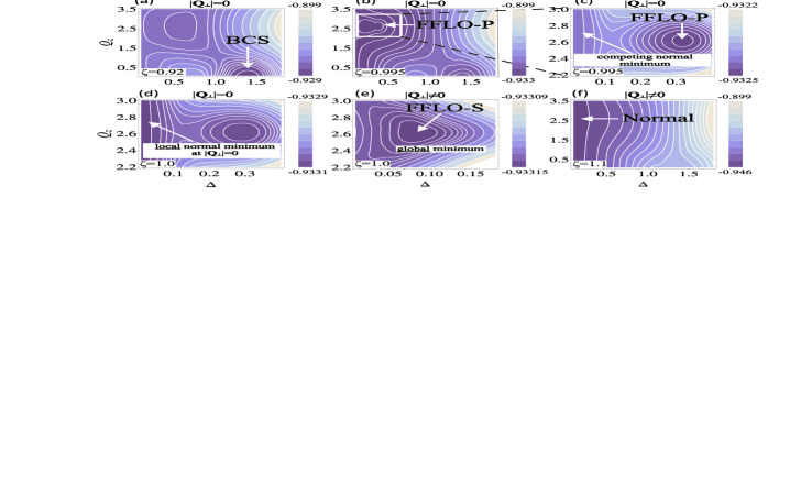
Figure 1: Several contour plots of the free energy as a function of the band gap $\Delta$ and the z-component of the FFLO wave vector $Q_{z}$. The value of the perpendicular component $\left|\mathbf{Q}_{\bot}\right|$ is held constant in each plot. Darker regions represent lower values of the free energy. Four different ground states can be identified: (a) a spin-balanced BCS superfluid $\left(\Delta\neq 0,Q_{z}=0,\left|\mathbf{Q}_{\bot}\right|=0\right)$, (b)/(c) the FFLO-P state $\left(\Delta\neq 0,Q_{z}\neq 0,\left|\mathbf{Q}_{\bot}\right|=0\right)$ , (e) the FFLO-S state $\left(\Delta\neq 0,Q_{z}\neq 0,\left|\mathbf{Q}_{\bot}\right|\neq 0\right)$, and (f) the normal state $\left(\Delta=0\right)$. In figures (c) and (d), the emergence of a local normal minimum that competes with the FFLO-P minimum is shown. There will however be no first order transition from FFLO-P to normal (c) $\rightarrow$ (d), because at the transition value of $\zeta$ ($\zeta=1.0$) where the normal minimum lies lower than the FFLO-P minimum (d), a new global minimum emerges at $\left|\mathbf{Q}_{\bot}\right|\neq 0$ (e). This means that the system becomes an FFLO-S state. The behavior shown in figures (c), (d) and (e) only occurs for $\mu\gtrapprox 3.0$. For lower values of $\mu$ the system makes a transition from BCS over FFLO-P to Normal. In all contour plots we used $\mu=4.44$, $V_{0}=6$, and $\lambda=1200$ $nm$.

This transition can be seen in Fig. 1 (b), where a second minimum emerges that starts to compete with the BCS minimum. This new minimum lies at $\left(\Delta\neq 0,Q_{z}\neq 0\right)$ but still at $\left|\mathbf{Q}_{\bot}\right|=0$ and is hence the FFLO-P state, which has a wave vector parallel to the periodic potential. The transition from BCS to FFLO-P is of first order, because there is a jump in the value of the band gap $\Delta$. When $\zeta$ increases further, one in principle expects the FFLO-P state to continuously go over into the normal state, as the band gap $\Delta$ will gradually decrease to zero when $\zeta$ increases. We indeed find this behavior at low values of $\mu$ ($\mu\lessapprox 3.0$). However, in the case of Fig. 1 (at $\mu=4.44$) the system behaves differently. When taking a closer look at the FFLO-P minimum in Fig. 1 (b), we see that the normal minimum (at $\Delta=0$) starts to compete with the FFLO-P minimum, which seems to imply a first order (FFLO-P)-to-normal transition (see Fig. 1 (c) and (d)). This is not what really happens though, because at the transition value of $\zeta$ ($\zeta=1.0$) where the normal minimum lies lower than the FFLO-P minimum (Fig. 1 (d)), a new global minimum emerges at $\left|\mathbf{Q}_{\bot}\right|\neq 0$ (Fig. 1 (e)), meaning that the system has made a transition from the FFLO-P state into the FFLO-S state. This shows that, at sufficiently high values of the total chemical potential $\mu$, the system can favor an FFLO state with a wave vector that lies skewed with respect to the direction of the 1D periodic potential. When $\zeta$ is increased further, the value of $\Delta$ for the FFLO-S state goes continuously to zero, and the system makes a transition into a normal interacting Fermi gas (Fig. 1 (f)).

III.2 The phase diagram as a function of the chemical potentials

The examples shown in Fig. 1 were only for one particular value of the total chemical potential $\mu$. When the free energy is minimized and therefore the ground state is determined for a large set of values for $\mu$ and $\zeta$, we obtain the phase diagram of the 3D imbalanced Fermi gas in the presence of a 1D periodic potential at zero temperature, as shown in Fig. 2.

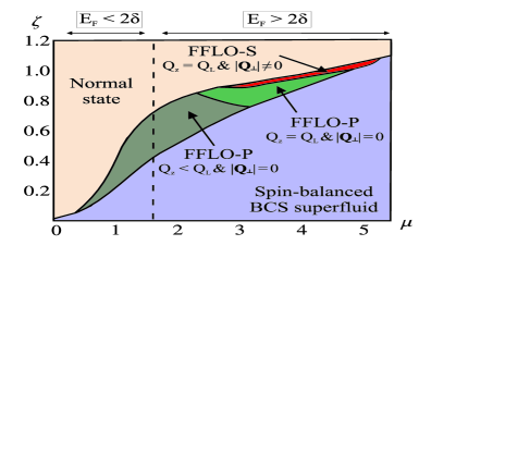
Figure 2: Phase diagram of a spin-imbalanced 3D Fermi gas in the presence of a 1D periodic potential, as a function of the total and imbalance chemical potentials $\mu$ and $\zeta$. The skewed FFLO state (FFLO-S) can be the ground state of the system but only at higher densities, when the Fermi energy lies above the energy corresponding to the top of the lowest Bloch band: $E_{F}>2\delta$. The region of the FFLO-P state (wave vector parallel to the periodic potential) is divided into two parts, where the z-component of the wave vector of FFLO $Q_{z}$ is either smaller or equal to the laser wave vector $Q_{L}$. The total FFLO region (FFLO-P + FFLO-S) is significantly larger than in the known 3D case without periodic potential. In this figure we used $V_{0}=6$ and $\lambda=1200~{}nm$ for the depth and wavelength of the periodic potential respectively.

This figure shows that the FFLO-S state can indeed be the ground state of the system. Furthermore, this state only occurs at higher densities, more specifically when the Fermi energy lies above the energy corresponding to the top of the first Bloch band: $E_{F}>2\delta$. The FFLO-P region can be subdivided into two regions. In one region, the z-component $Q_{z}$ of the wave vector of the FFLO-P state is smaller than the wave vector of the periodic potential $Q_{L}$. In the other region, this z-component equals the wave vector of the potential. The FFLO-S state only occurs when $Q_{z}=Q_{L}$. This observation along with the fact that the FFLO-S state only occurs when $E_{F}>2\delta$ will be explained in the next subsection, where we illustrate the FFLO pairing mechanism in momentum space. As we have shown before 22 - Devreese Klimin Tempere , a striking feature of the phase diagram in Fig. 2 is the significant increase in the area of the FFLO state, compared to the case of a 3D Fermi gas without periodic potential. In the latter case, the FFLO area would barely be visible on the scale of Fig. 2. This is a result of the fact that the periodic potential lowers the energy for the formation of the FFLO state, relative to the BCS and the normal state.

III.3 The influence of the periodic potential on the pairing mechanism of the FFLO state

The occurrence of the FFLO-S state in the $\left(\mu,\zeta\right)$-phase diagram may appear rather counterintuitive at first sight. Indeed, due to the presence of the periodic potential, it costs less energy to form Cooper pairs with a momentum that lies parallel to the periodic potential as compared to Cooper pairs with a momentum that lies skewed with respect to this potential. To explain why the FFLO-S state can be the ground state of the system, we give a qualitative description of the pairing mechanism of the FFLO state in the system under consideration. An insightful visualization of this pairing mechanism is to plot the Fermi surfaces of up and down particles in momentum space, as shown in Fig. 3. In this figure, eight different pictures each show the Fermi surfaces of up and down spins at given values of the chemical potentials $\mu$ and $\zeta$. Around each Fermi surface, a band of size $2\Delta$ is indicated. Only particles that lie within these ’pairing bands’ can participate in superfluid pairing. This means that there has to be an overlap between the pairing bands of up and down spins for superfluid pairs to exist. Each picture in Fig. 3 corresponds to a point on the phase diagram in Fig. 2. For reasons of clarity, this phase diagram is reproduced in the inset of figure 3, where the points corresponding to each of the eight pictures are indicated by small black filled circles. The different pictures are subdivided in three subsets A, B and C, which represent distinct physical situations.

Subset A corresponds to the situation where the Fermi energy of the system lies lower than the energy of the top of the lowest Bloch band $\left(E_{F}<2\delta\right)$. In this case, both the Fermi surfaces of up- and down-particles are approximately spherical and the pairing mechanism is roughly the same as in the known 3D situation 29 - Chevy . Picture A1 shows a spin-balanced superfluid, where the Fermi surfaces of both particles overlap completely since there is no polarization. In picture A2, a nonzero polarization has been introduced by increasing the chemical potential $\zeta$ above a certain critical value. As a consequence, the system has made a transition into the FFLO-P state, where the magnitude of the wave vector of the FFLO state is such that it partially re-aligns both Fermi surfaces so that a maximal number of FFLO-type pairs can be formed. Figure A2 shows the essence of the FFLO state: granting a nonzero momentum to all pairs requires energy, but this energy is gained back because more bosonic pairs can be formed. The presence of the periodic potential favors the FFLO state, since it becomes energetically more favorable to translate the minority Fermi surface along the direction of the potential compared to any other direction. This is because in this direction the energy dispersion (given by expression (3)) is flatter than a free particle dispersion, which means that it costs less energy to bridge a gap of given size in momentum space. In the case of a 3D Fermi gas, the energy dispersion is quadratic in all dimensions, so adding the periodic potential lowers the energy for the FFLO state compared to the BCS state and the normal state. This explains the significant enlargement of the FFLO region in the phase diagram in Fig. 2 compared to the case of a 3D Fermi gas.

Aside from this energy lowering property for the FFLO state, the presence of the periodic potential has additional effects. This becomes more prominent when the density of the system is increased and the Fermi energy becomes larger than the energy corresponding to the top of the lowest Bloch band $\left(E_{F}>2\delta\right)$.

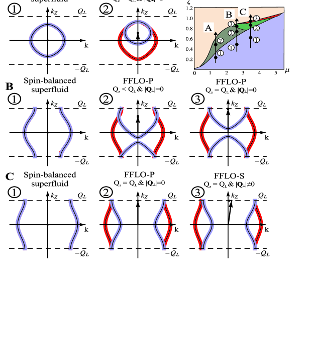
Figure 3: Visualization of the pairing mechanism of the FFLO state in the presence of a 1D periodic potential for different values of the chemical potentials. In each picture the Fermi surfaces of up and down spins are shown in momentum space. Around each Fermi surface a band of thickness $2\Delta$ is indicated. Only particles that lie in these bands can form superfluid pairs. The corresponding points in the $\left(\mu,\zeta\right)$-phase diagram are indicated in the inset. In subset A, the Fermi energy lies lower than the energy corresponding to the top of the lowest Bloch band. In subset B and C, the Fermi energy lies above the energy of the top of the lowest Bloch band. When polarization is introduced, the system becomes FFLO-P and the minority Fermi surface is translated by an amount $Q_{z}$ (A2). When the density or the polarization increases, the wave vector of FFLO increases likewise in order to keep both Fermi surfaces aligned (B2). The extreme case is shown in B3 and C2, where $Q_{z}=Q_{L}$. At even higher density (subset C), the FFLO wave vector becomes skewed with respect to the direction of the periodic potential (C3). This costs more energy to translate the Fermi surface, but more pairs can be formed because the overlap between pairing bands is increased. This lowers the energy enough for the FFLO-S state to become the ground state.

An example of this situation is shown in subset B in Fig. 3. Here the value of $\mu$ and hence also the density of the system is larger compared to subset A. This can for example be seen in picture B1, which represents a spin-balanced superfluid. In this picture, both Fermi surfaces are no longer spherical because they have ’hit’ the edge of the first Brillouin zone. When polarization is introduced, the system again becomes of the FFLO-P type, as shown in pictures B2 and B3. Here it becomes clear why the wave vector of the FFLO state increases when the polarization is increased. In order to maximize the overlap between the pairing bands of up and down spins, the bulge (in the $k_{z}$ direction) in the Fermi surface of the down spins must align with the waist (in the $k_{z}$ direction) of the Fermi surface of the up spins. This requires that the Fermi surface of the down spins be translated increasingly if the polarization is increased. In picture B3, the polarization is large enough so that the FFLO wave vector becomes equal to the wave vector of the periodic potential, as indicated by the arrow in this picture. This is the largest possible value that the FFLO wave vector can have. Any increase in the magnitude of this vector would simply be equivalent to an equal decrease in the magnitude of this vector.

In both subsets A and B, the FFLO wave vector always lies parallel to the direction of the periodic potential. In subset C however, a case is shown where this no longer applies. Here the density has increased even more compared to subset B, as can be seen for instance in picture C1. Picture C2 shows another FFLO-P case, where $Q_{z}=Q_{L}$. When the polarization is increased compared to this case, the majority Fermi surface will widen and the minority Fermi surface will narrow further. This will inevitably result in a decrease in overlap between the pairing bands of up- and down-spins, thus raising the energy of the FFLO state compared to the normal state. As can be seen in picture C3, the FFLO state can solve this problem by forcing its wave vector to lie skewed with respect to the direction of the periodic potential. Now it becomes intuitively clear why the FFLO-S state can be the ground state of the system. Although it costs more energy to add a perpendicular component to the FFLO wave vector (since the component $Q_{z}$ remains equal to the laser wave vector $Q_{L}$), more superfluid pairs can be formed because the overlap between the Fermi surfaces of up and down spins is increased, relative to the case where $\left|\mathbf{Q}_{\bot}\right|=0$. This is only true when the density is large enough so that the Fermi energy lies above the energy of the top of the lowest Bloch band ($E_{F}>2\delta$) and when $Q_{z}=Q_{L}$ (subset C in 3), which explains why the FFLO-S state only occurs on that part of the $\left(\mu,\zeta\right)$-phase diagram. One can see the FFLO-S state as a final straw at which the FFLO state will grasp to maintain its existence in a highly polarized Fermi gas. If the polarization keeps increasing, the cost in energy will eventually become too high and the normal state will be energetically more favorable.
Experimentally, the FFLO-S state can provide an additional signature for observing FFLO superfluidity, in comparison with the FFLO-P state. When attempting to observe the FFLO-P state, it may be hard to distinguish this state from the 1D periodic potential. This is because both share the same Bragg peaks in momentum space when the FFLO state is optimally enhanced Acknowledgement Zwierlein . The advantage of FFLO-S for experimental detection is that it has an additional momentum component that lies perpendicular to the momentum component of the periodic potential. Observing this extra momentum component can provide direct evidence of polarized superfluidity of the FFLO type.

IV Conclusion

In this paper, we have studied the effect of a 1D periodic potential on the pairing mechanism of the FFLO state in a 3D Fermi gas. Starting from the partition sum of the system, the free energy was derived within the saddle-point approximation. By choosing a suitable saddle point, we included the FFLO state in our description, were the FFLO wave vector was allowed to lie in an arbitrary direction. Minimizing the free energy with respect to the band gap and the FFLO wave vector allowed to study the different competing ground states of the system. This subsequently led to the phase diagram as a function of the total and the imbalance chemical potential. From this phase diagram we have found that, surprisingly, the wave vector of the FFLO state can lie skewed (FFLO-S) with respect to the direction along which the periodic potential lies. Furthermore, we showed that this FFLO-S state only occurs when the Fermi energy of the system lies above the energy corresponding to the top of the lowest Bloch band. To gain a deeper understanding of this counterintuitive phenomenon, we explored the pairing mechanism of the FFLO state by studying the Fermi surfaces of the spin up and spin down fermions in momentum space. This visualization showed that the FFLO-S state can be energetically favorable with respect to the FFLO-P state, because tilting the FFLO wave vector can result in an increase in the overlap between the pairing bands of up and down spins. We argued that, experimentally, the FFLO-S state can provide an additional signature for FFLO superfluidity in a 3D Fermi gas. This is because this state has an additional perpendicular momentum component, which allows it to be more easily distinguished from the 1D periodic potential than the FFLO-P state, since the latter shares the same Bragg peaks with the potential when the FFLO state is optimally enhanced.

Acknowledgements

The authors would like to thank Martin Zwierlein and Hagen Kleinert for helpful suggestions and comments. We wish to thank Randy Hulet, Carlos Sá de Melo and Sergei Klimin for interesting and stimulating discussions. One of the authors (JPAD) gratefully acknowledges a Ph. D. fellowship of the Research Foundation - Flanders (FWO-V). This work was supported by FWO-V projects G.0356.06, G.0370.09N, G.0180.09N, G.0365.08.

Appendix A Analytic treatment of the free energy

To the best of our knowledge, it is impossible to calculate all integrals in expression (8) for the free energy analytically. It is however possible to solve the radial part exactly. To accomplish this, we introduce a cutoff $K_{c}$ in the integral over $k_{\bot}$ and divide expression (8) into three parts:

$$\Omega_{sp}=-\frac{1}{\left(2\pi\right)^{3}}\left(I_{1}+I_{2}+I_{3}\right)+\frac{\left|\Delta\right|^{2}}{8\pi},$$ (13)

where the three different parts are given by

$$\left\{\begin{array}[c]{l}I_{1}=\int_{0}^{2\pi}d\theta\int_{-Q_{L}}^{Q_{L}}dk_{z}\left(\int_{0}^{k_{1}}+...+\int_{k_{N-1}}^{k_{N}}+\int_{k_{N}}^{K_{C}}\right)dk_{\bot}~{}k_{\bot}\max\left(E_{\mathbf{k},\mathbf{Q}},\left|\zeta_{\mathbf{k},\mathbf{Q}}\right|\right)\\ I_{2}=\int_{0}^{2\pi}d\theta\int_{-Q_{L}}^{Q_{L}}dk_{z}\int_{K_{C}}^{\infty}dk_{\bot}~{}k_{\bot}\left(E_{\mathbf{k},\mathbf{Q}}-\xi_{\mathbf{k},\mathbf{Q}}-\frac{\left|\Delta\right|^{2}}{2\left\{k_{\bot}^{2}+\delta\left[1-\cos\left(\frac{\pi k_{z}}{Q_{L}}\right)\right]\right\}}\right)\\ I_{3}=\int_{0}^{2\pi}d\theta\int_{-Q_{L}}^{Q_{L}}dk_{z}\int_{0}^{K_{C}}dk_{\bot}~{}k_{\bot}\left(-\xi_{\mathbf{k},\mathbf{Q}}-\frac{\left|\Delta\right|^{2}}{2\left\{k_{\bot}^{2}+\delta\left[1-\cos\left(\frac{\pi k_{z}}{Q_{L}}\right)\right]\right\}}\right)\end{array}\right.,$$ (14)

and the shorthand notations (9) - (11) are used. In the first part $I_{1}$, the different values $k_{1},...,k_{N}$ represent the roots of the equation $E_{\mathbf{k},\mathbf{Q}}=$ $\left|\zeta_{\mathbf{k},\mathbf{Q}}\right|$, solved with respect to $k_{\bot}$. These roots are solutions of a fourth order equation and are rather cumbersome to treat analytically, so it is best to calculate these values numerically. The main purpose of the division in (14) is to separate the logarithmic divergence in the integrand in $I_{3}$ $\left(\text{when }k_{z}=0,k_{\bot}=0\right)$ so that this part can be treated analytically. The terms in $I_{2}$ have to stay together because they all diverge for $k_{\bot}\rightarrow\infty$, and they only cancel out when combined. We now proceed to treat each part analytically to the furthest possible extent.

To calculate the integral over $k_{\bot}$ in $I_{1}$ analytically we consider two distinct cases. If $E_{\mathbf{k},\mathbf{Q}}>\left|\zeta_{\mathbf{k},\mathbf{Q}}\right|$ the result is given by

$$I_{1} =\int_{0}^{2\pi}d\theta\int_{-Q_{L}}^{Q_{L}}dk_{z}\left(\sum_{i=1}^{N+2}\right)$$

$$\times\left\{\frac{\Delta^{2}}{4}\log\left(\frac{\left[K_{i+1}^{2}+A\left(k_{z}\right)\right]+\sqrt{\left[K_{i+1}^{2}+A\left(k_{z}\right)\right]^{2}+\Delta^{2}}}{\left[K_{i}^{2}+A\left(k_{z}\right)\right]+\sqrt{\left[K_{i}^{2}+A\left(k_{z}\right)\right]^{2}+\Delta^{2}}}\right)\right.$$

$$+\frac{1}{4}\left(\left[K_{i+1}^{2}+A\left(k_{z}\right)\right]\sqrt{\left[K_{i+1}^{2}+A\left(k_{z}\right)\right]^{2}+\Delta^{2}}\right.$$

$$\left.\left.-\left(K_{i}^{2}+A\right)\sqrt{\left(K_{i}^{2}+A\right)^{2}+\Delta^{2}}\right)\vskip 12.0pt plus 4.0pt minus 4.0pt\right\},$$ (15)

where the set of values $K_{i}=\left(0,k_{1},...,k_{N},K_{c}\right)$ consists of all roots of equation $E_{\mathbf{k},\mathbf{Q}}=$ $\left|\zeta_{\mathbf{k},\mathbf{Q}}\right|$, complemented with zero and the cutoff $K_{c}$. In the other case when $E_{\mathbf{k},\mathbf{Q}}<\left|\zeta_{\mathbf{k},\mathbf{Q}}\right|$ the result is

$$I_{1} =\int_{0}^{2\pi}d\theta\int_{-Q_{L}}^{Q_{L}}dk_{z}\left(\sum_{i=1}^{N+2}\right)$$

$$\times\left[\begin{array}[c]{c}\delta_{Q_{\bot}\cos\left(\theta\right),0}\left(\frac{\left|B\left(k_{z}\right)\right|}{2}\left(K_{i+1}^{2}-K_{i}^{2}\right)\right)\\ +\left(\left(1-\delta_{Q_{\bot}\cos\left(\theta\right),0}\right)\left\{\Theta\left[Q_{\bot}\cos\left(\theta\right)\right]-\Theta\left[-Q_{\bot}\cos\left(\theta\right)\right]\right\}\vskip 6.0pt plus 2.0pt minus 2.0pt\right)\end{array}\right.$$ (18)

$$\times\left.\left(\begin{array}[c]{c}\left(\Theta\left[K_{i}-k_{np}\right]-\Theta\left[k_{np}-K_{i+1}\right]\right)\\ \times\left(\frac{B\left(k_{z}\right)}{2}\left(K_{i+1}^{2}-K_{i}^{2}\right)+\dfrac{Q_{\bot}\cos\left(\theta\right)}{3}\left(K_{i+1}^{3}-K_{i}^{3}\right)\right)\\ +\Theta\left[k_{np}-K_{i}\right]\Theta\left[K_{i+1}-k_{np}\right]\\ \times\left(\frac{B\left(k_{z}\right)}{2}\left(K_{i+1}^{2}-2k_{np}^{2}+K_{i}^{2}\right)+\dfrac{Q_{\bot}\cos\left(\theta\right)}{3}\left(K_{i+1}^{3}-2k_{np}^{3}+K_{i}^{3}\right)\right)\end{array}\right)\right],$$ (23)

where the following shorthand notations were used

$$A\left(k_{z}\right) =\delta\left[1-\cos\left(\frac{\pi k_{z}}{Q_{L}}\right)\cos\left(\frac{\pi}{2}\frac{Q_{z}}{Q_{L}}\right)\right]-\left(\mu-\frac{Q_{\bot}^{2}}{4}\right)$$ (24)

$$B\left(k_{z}\right) =\zeta-\delta\sin\left(\frac{\pi k_{z}}{Q_{L}}\right)\sin\left(\frac{\pi}{2}\frac{Q_{z}}{Q_{L}}\right)$$ (25)

$$k_{np} =\frac{-B\left(k_{z}\right)}{Q_{\bot}\cos\left(\theta\right)}$$ (26)

In both expressions (15) and (23) the set of values $K_{i}=\left(0,k_{1},...,k_{N},K_{c}\right)$ consists of all the roots of equation $E_{\mathbf{k},\mathbf{Q}}=$ $\left|\zeta_{\mathbf{k},\mathbf{Q}}\right|$, complemented with zero and with the cutoff $K_{c}$.

Expression $I_{2}$ can also be partly calculated analytically. Here we simply state the result

$$I_{2}=\frac{\pi}{2}\int_{-Q_{L}}^{Q_{L}}dk_{z}\left(\begin{array}[c]{c}\left(\dfrac{-\Delta^{2}\left[K_{C}^{2}+A\left(k_{z}\right)\right]}{\left[K_{C}^{2}+A\left(k_{z}\right)\right]+\sqrt{\left[K_{C}^{2}+A\left(k_{z}\right)\right]^{2}+\Delta^{2}}}\right)+\dfrac{\Delta^{2}}{2}\\ +\Delta^{2}\log\left(\dfrac{2\left(K_{C}^{2}+\varepsilon\left(k_{z}\right)\right)}{\left[K_{C}^{2}+A\left(k_{z}\right)\right]+\sqrt{\left[K_{C}^{2}+A\left(k_{z}\right)\right]^{2}+\Delta^{2}}}\right)\end{array}\right),$$ (27)

with

$$\varepsilon\left(k_{z}\right)=\delta\left[1-\cos\left(\frac{\pi k_{z}}{Q_{L}}\right)\right].$$ (28)

The last part $I_{3}$ contains a logarithmic divergence in the integrand, but fortunately we found that this expression can be calculated analytically:

$$I_{3} =-\pi K_{C}^{2}Q_{L}\left\{K_{C}^{2}+2\left[\delta-\left(\mu-\frac{Q_{\bot}^{2}}{4}\right)\right]\right\}$$

$$+Q_{L}\left|\Delta\right|^{2}\pi\log\left(\frac{\delta}{\left(K_{C}^{2}+\delta\right)+\sqrt{K_{C}^{4}+2K_{C}^{2}\delta}}\right).$$ (29)

References

- (1) I. Bloch, Nat. Phys. 1, 23 (2005).
- (2) M. Greiner and S. Fölling, Nature (London) 453, 736 (2008).
- (3) M. Greiner, C.A. Regal, and D.S. Jin, Nature 426, 537 (2003).
- (4) M.W. Zwierlein, C.A. Stan, C.H. Schunck, S.M.F. Raupach, S. Gupta, Z. Hadzibabic, and W. Ketterle, Phys. Rev. Lett. 91, 250401 (2003).
- (5) S. Jochim, M. Bartenstein, A. Altmeyer, G. Hendl, S. Riedl, C. Chin, J. Hecker Denschlag, and R. Grimm, Science 302, 5653 (2003).
- (6) T. Bourdel, L. Khaykovich, J. Cubizolles, J. Zhang, F. Chevy, M. Teichmann, L. Tarruell, S.J.J.M.F. Kokkelmans, and C. Salomon, Phys. Rev. Lett. 93, 050401 (2004).
- (7) G.B. Partridge, K.E. Strecker, R.I. Kamar, M.W. Jack, and R.G. Hulet, Phys. Rev. Lett. 95, 020404 (2005).
- (8) C.A. Regal, M. Greiner, and D.S. Jin, Phys. Rev. Lett. 92, 040403 (2004).
- (9) M.W. Zwierlein, C.A. Stan, C.H. Schunck, S.M.F. Raupach, A.J. Kerman, and W. Ketterle, Phys. Rev. Lett. 92, 120403 (2004).
- (10) M.W. Zwierlein, J.R. Abo-Shaeer, A. Schirotzek, C.H. Schunck, and W. Ketterle, Nature 435, 1047 (2005).
- (11) C. Chin, R. Grimm, P. Julienne, and E. Tiesinga, Rev. Mod. Phys. 82, 1225 (2010).
- (12) M. Bartenstein, A. Altmeyer, S. Riedl, S. Jochim, C. Chin, J.H. Denschlag, and R. Grimm, Phys. Rev. Lett. 92, 120401 (2004).
- (13) A.M. Clogston, Phys. Rev. Lett. 9, 266 (1962); B.S. Chandrasekhar, Appl. Phys. Lett. 1, 7 (1962).
- (14) M.W. Zwierlein, A. Schirotzek, C.H. Schunck, and W. Ketterle, Science 311, 492 (2006).
- (15) G.B. Partridge, W. Li, R.I. Kamar, Y.A. Liao, and R.G. Hulet, Science 311, 503 (2006).
- (16) P. Fulde and R.A. Ferrell, Phys. Rev. 135, A550 (1964).
- (17) A.I. Larkin and Y.N. Ovchinnikov, Zh. Eksp. Teor. Fiz. 47, 1136 (1964) [Sov. Phys. JETP 20, 762 (1965)].
- (18) T. Mizushima, K. Machida, and M. Ichioka, Phys. Rev. Lett. 94, 060404 (2005); D.E. Sheehy and L. Radzihovsky, ibid. 96, 060401 (2006); J. Kinnunen, L.M. Jensen, and P. Törmä, ibid. 96, 110403 (2006); K. Machida, T. Mizushima, and M. Ichioka, ibid. 97, 120407 (2006); P. Castorina, M. Grasso, M. Oertel, M. Urban, and D. Zappalà, Phys. Rev. A 72, 025601 (2005); N. Yoshida and S.-K. Yip, ibid. 75, 063601 (2007); W. Zhang and L.-M. Duan, ibid. 76, 042710 (2007); T.K. Koponen, T. Paananen, J.-P. Martikainen, M.R. Bakhtiari, and P. Törmä, New J. Phys. 10, 045014 (2008).
- (19) K. Yang, Phys. Rev. B 63, 140511(R) (2001); G. Orso, Phys. Rev. Lett. 98, 070402 (2007); M.M. Parish, S.K. Baur, E.J. Mueller, and D.A. Huse, idib. 99, 250403 (2007); H. Hu, X.-J. Liu, P.D. Drummond, ibid. 98, 070403 (2007); G.G. Batrouni, M.H. Huntley, V.G. Rousseau, and R.T. Scalettar, ibid. 100,116405 (2008); A.E. Feiguin and F. Heidrich-Meisner, Phys. Rev. B 76, 220508(R) (2007); M. Rizzi, M. Polini, M.A. Cazalilla, M.R. Bakhtiari, M.P Tosi, and R. Fazio, ibid. 77, 245105 (2008).
- (20) Y. Liao, A. S. C. Rittner, T. Paprotta, W. Li, G. B. Partridge, R. G. Hulet, S. K. Baur, and E. J. Mueller, Nature 467, 567 (2010).
- (21) H. Hu and X.J. Liu, Phys. Rev. A 73, 051603(R) (2006).
- (22) D.E. Sheehy and L. Radzihovsky, Ann. of Phys. 322, 1790 (2007); L. Radzihovsky and D.E. Sheehy, Rep. Prog. Phys. 73, 076501 (2010).
- (23) T.K. Koponen, T. Paananen, J.-P. Martikainen, and P. Törmä, Phys. Rev. Lett. 99, 120403 (2007); D.-H. Kim, J.J. Kinnunen, J.-P. Martikainen, and P. Törmä, ibid. 106, 095301 (2011).
- (24) Y.L. Loh and N. Trivedi, Phys. Rev. Lett. 104, 165302 (2010).
- (25) Jeroen P.A. Devreese, S.N. Klimin, and J. Tempere, Phys. Rev. A 83, 013606 (2011).
- (26) H. Kleinert, Path Integrals in Quantum Mechanics, Statistics, Polymer Physics, and Financial Markets, 5th ed. (World Scientific, Singapore, 2002).
- (27) C.A.R. Sá de Melo, M. Randeria, and J.R. Engelbrecht, Phys. Rev. Lett. 71, 3202 (1993).
- (28) Jeroen P.A. Devreese, M. Wouters, and J. Tempere, J. Phys. B: At. Mol. Opt. Phys. 44, 115302 (2011).
- (29) W. Zwerger, J. Opt. B: Quantum Semiclass. Opt. 5 (2003) S9–S16.
- (30) H. Kleinert, EJTP 8, 57 (2011).
- (31) R.P. Feynman and H. Kleinert, Phys. Rev. A 34, 5080 (1986).
- (32) F. Chevy and C. Mora, Rep. Prog. Phys. 73, 112401(2010).
- (33) We would like to thank Martin Zwierlein for pointing out this fact to us.