The MOLDY short-range molecular dynamics package

Abstract

We describe a parallelised version of the MOLDY molecular dynamics program. This Fortran code is aimed at systems which may be described by short-range potentials and specifically those which may be addressed with the embedded atom method. This includes a wide range of transition metals and alloys. MOLDY provides a range of options in terms of the molecular dynamics ensemble used and the boundary conditions which may be applied. A number of standard potentials are provided, and the modular structure of the code allows new potentials to be added easily. The code is parallelised using OpenMP and can therefore be run on shared memory systems, including modern multicore processors. Particular attention is paid to the updates required in the main force loop, where synchronisation is often required in OpenMP implementations of molecular dynamics. We examine the performance of the parallel code in detail and give some examples of applications to realistic problems, including the dynamic compression of copper and carbon migration in an iron-carbon alloy.

PROGRAM SUMMARY

Manuscript Title: The MOLDY short-range molecular dynamics package
Authors: G J Ackland K D’Mellow S L Daraszewicz D J Hepburn M Uhrin K Stratford
Program Title: MOLDY
Journal Reference:
Catalogue identifier:
Licensing provisions: GNU General Public License Version 2
Programming language: Fortran 95 / OpenMP
Computer: any
Operating system: any
RAM: 100 MB or more
Number of processors used: any
Supplementary material: Requires OpenMP for parallel execution
Keywords: molecular dynamics; embedded atom method; openmp
PACS: 71.15.Pd, 71.20.Be
Classification: 7.7 Other Condensed Matter inc. Simulation of Liquids and Solids
Nature of problem: Moldy addresses the problem of many atoms (of order $10^{6}$) interacting via a classical interatomic potential on a timescale of microseconds. It is designed for problems where statistics must be gathered over a number of equivalent runs, such as measuring thermodynamic properities, diffusion, radiation damage, fracture, twinning deformation, nucleation and growth of phase transitions, sputtering etc. In the vast majority of materials, the interactions are non-pairwise, and the code must be able to deal with many-body forces.
Solution method: Molecular dynamics involves integrating Newton’s equations of motion. MOLDY uses verlet (for good energy conservation) or predictor-corrector (for accurate trajectories) algorithms. It is parallelised using open MP. It also includes a static minimisation routine to find the lowest energy structure. Boundary conditions for surfaces, clusters, grain boundaries, thermostat (Nose), barostat (Parrinello-Rahman), and externally applied strain are provided. The initial configuration can be either a repeated unit cell or have all atoms given explictly. Initial velocities are generated internally, but it is also possible to specify the velocity of a particular atom. A wide range of interatomic force models are implemented, including embedded atom, morse or Lennard Jones. Thus the program is especially well suited to calculations of metals.
Restrictions: The code is designed for short-ranged potentials, and there is no Ewald sum. Thus for long range interactions where all particles interact with all others, the order-N scaling will fail. Different interatomic potential forms require recompilation of the code.
Additional comments: There is a set of associated open-source analysis software for postprocessing and visualisation. This includes local crystal structure recognition and identification of topological defects.
Running time: A set of test modules for running time are provided. The code scales as order N. The parallelisation shows near-linear scaling with number of processors in a shared memory environment. A typical run of a few tens of nanometers for a few nanoseconds will run on a timescale of days on a multiprocessor desktop.

1 Introduction

Classical molecular dynamics (MD), which solves Newton’s laws of motion for a system made up of atoms and/or molecules, is a powerful and widely used tool to study both simple and complex systems. With the power of modern computers, these systems can range in size from a few thousand to many millions of atoms. Of particular interest for modern hardware are codes which can take advantage of multicore processors and increasingly accelerators, such as graphics processing units (GPUs).

A number of well-established classical MD packages exist which may be used to simulate very large systems in various contexts [e.g., LAMMPS, DL_POLY, NAMD]. These codes are able to address large systems by means of domain decomposition and message passing, usually via the Message Passing Interface (MPI). Some of these codes are important for general purposes, while others are more fashioned for particular fields, such as large biomolecules or proteins.

The code described here, MOLDY, is one specifically developed with metals and alloys in mind. This allows the code to be used for a wide range of problems of practical interest, such as the properties of materials undergoing deformation, defect propagation and radiation damage. It is not our intention to put forward a replacement for codes of the type mentioned above, but to provide a complementary option which allows users to simulate modestly large systems on desktop machines. The increasing proliferation of multicore machines makes OpenMP an ideal route to allow users less familiar with MPI the chance to adapt the code incrementally without the additional complexity involved with message passing. Further, the inclusion of standard directives in future versions of OpenMP to distribute work to accelerated hardware such as graphical processing units (GPUs) would place the code in a good position to access these resources.

The code is a direct descendant of a Fortran code “Moldy” which was first developed at the United Kingdom Atomic Energy Research Establishment [1, 2], with conventional constant volume and constant pressure ensembles and deforming systems under constant stress using the extended Lagrangian formulation of Parrinello and Rahman [4]. In Moldy, the atoms interact via short-range pairwise potentials and are free of bond constraints or long-range interactions. These two simplifications are retained in the current version. The code was extended to include the embedded atom method [5], or Finnis-Sinclair potentials [6]. This feature specifically aims the code at the simulation of metals and alloys.

In retaining Fortran as the language of the updated version, we have made the decision to restrict development to level of the Fortran 1995 standard. This is for reasons of portability: compiler support for some features of later Fortran standards is currently not complete. This means some design compromises from a software engineering point of view. For example, an abstract potential type, or class, might have been preferable for extensibility and flexibility. Instead, at the moment, the potential is introduced at compile time as a fixed module, so the code is recompiled for each different material. However, the existing design does not preclude refactoring to make use of these attractive language features in future. We hope the level of compiler support for Fortran 2003 features will improve rapidly in the near future.

In the following section we provide a brief background on molecular dynamics which makes clear the issues addressed in the paper. Section 3 goes on to discuss the structure of the code and in particular how the potentials should be represented. A number of different potentials are included as examples. Importantly, this section also discusses the strategy for the parallelisation of the force loop using OpenMP. Section 4 gives an overview of how the code is run in practice and how the user deals with input and output. Section 5 shows results for the parallel performance of the code for a number of idealised problems and considers a number of simple example applications. These applications present an opportunity for visualisation and local crystal structure determination, which are provided as part of the package. A summary and conclusions are presented in Section 6.

2 Theoretical background

On account of the screening properties of the conduction electrons, metals can be described by short range interatomic potential. This offer significant advantages for molecular dynamics simulations, in particular since each atom interacts only with a finite number of neighbours the computer time to calculate forces scales as $O(N)$ rather than $O(N^{2})$ for generalised long ranged forces, or $O(N^{1.5})$/$O(NlogN$ for Coulombic Ewald sums or fast multipole techniques.

For simulations of large numbers of atoms, it is essential that the electronic degrees of freedom are integrated out, and forces depend only on the atomic positions. However, since the electrons are delocalised, the forces cannot be simply pairwise interactions between atoms. The delocalisation also suggests that an expansion in two-, three, four-body terms may not converge quickly, if at all [7]. Since 1984 potentials involving a function of some measure of the local density have become the methods of choice. The two most prominent are the Embedded Atom (EAM) and the second-moment tight-binding methods, also called Finnis-Sinclair (FS) [6]. In these the cohesive energy is written as:

$$U_{coh}=\sum_{i}\left(\sum_{j}V_{ij}(r_{ij})+F_{i}[\sum_{j}\phi_{ij}(r_{ij})]\right)$$ (1)

where $V$ and $\phi$ are short-ranged pairwise potentials, and $F$ is a function of the sum of $\phi$’s. The form of the second term means that an expansion of the potential in $n$-atom terms does not converge [7].

The interpretations of $\phi$’s are subtly different. In EAM the $\phi_{ij}=\phi_{j}\neq\phi_{i}$ represents the electron density from the atom $j$ at site $i$ - it depends only on the type of atom at $j$. In FS $\phi_{ij}=\phi_{ji}$ is the square of the tight binding hopping integral between $j$ and $i$ - it depends on both types of atom [5, 8]. In both cases $\phi$ is a function only of the interatomic distance. Similarly the EAM “embedding function” $F_{i}$ depends on the atom at site $i$, while in the FS picture, $F$ is a universal function for a canonical $d$-band, independent of atom types - the square root. In practice, these distinctions only become important when more than one atomic type is considered.

A number of potentials which appear to be different actually take the same form as Eq. 1. These include the “magnetic” type potentials[9, 10], rescaled potentials[11] and the Metallic-Covalent FeC potential of Hepburn-Ackland [12].

Similarly, simple pairwise potentials such as Morse or Lennard-Jones can be cast into this form by setting $F(\rho)=0$.

The form of the potential allows one to define the “energy of an atom”. This concept is both useful and meaningless. It is useful because deviations from the mean value can be used to highlight defects or hotspots in a simulation, but meaningless because the physically meaningful quantities, total energy and forces, are independent of how the energy is partitioned between atoms.

2.1 Ensembles

The code implements several different ensembles.

The “Total Energy” reported by MOLDY comprises only the kinetic energy of the movable particles and the cohesive energy of the system. However the additional degrees of freedom of the extended Lagrangian introduced by the thermostat and barostat can exchange energy with the system. Thus the only ensemble in which total energy is conserved is NVEp, i.e. without barostat or thermostat.

2.1.1 Molecular dynamics (microcanonical) NVEp

The standard “molecular dynamics” ensemble is NVEp - constant particle number, volume, energy and momentum (p=0). The momentum constraint distinguishes it slightly from microcanonical NVE.

2.1.2 Thermostat NVTp

The Nose-Hoover [13, 14] thermostat can be applied to produce an NVTp canonical ensemble. This couples the system to an external heat bath. The temperature is defined by the kinetic energy via the relation:

$$\sum_{i}\frac{\bf p_{i}^{2}}{2m_{i}}=\frac{3N-3}{2}k_{B}T$$

where $k_{B}$ is the Boltzmann constant, $m_{i}$ and $\bf p_{i}$ are the particle masses and momenta and (3N-3) is the number of degrees of freedom once total momentum is conserved.

The Nose-Hoover thermostat is an extended Hamiltonian, which can be interpreted as an external heat reservoir, with an additional degree of freedom. This heat reservoir controls the temperature through exchange of kinetic energy with the system. To define a heat bath kinetic energy we introduce an effective mass $Q_{s}$ and momentum $\pi_{s}$. The equations of motion are then

$$\frac{d\bf r_{i}}{dt}=\frac{\bf p_{i}}{m_{i}},$$

$$\frac{d\bf p_{i}}{dt}=-\frac{\partial U}{\partial\bf q_{i}}-\pi_{s}{\bf p_{i}},$$

$$Q_{s}\frac{d\pi_{s}}{dt}=\sum_{i}\frac{{\bf p_{i}}^{2}}{2m_{i}}-(3N-3)kT.$$

Thus $\pi$ is the degree of freedom associated with the thermostat, effectively a thermodynamic friction and $Q_{s}$ is “thermal inertia”, which determines the rate of heat transfer and how closely the temperature is maintained near to the target temperature $T_{opt}$. The value of $Q_{s}$ depends on the heat conduction in the system and must be specified in the input to the code. It is possible to choose $Q_{s}$ to reproduce missing effects such as electronic heat conduction.

2.1.3 Barostat NPTp

The Parrinello-Rahman method [4] is implemented for simulations in the NPEp (or with Nose, NPTp) ensemble. There are a number of anomalies in that paper[15, 16, 17], including lack of rotational invariance and missing cross terms in the derivatives, and these are reproduced faithfully by the code.

The positions $r_{i}$ are written as a product of fractional coordinates ${\bf x_{i}}$ and a 3$\times$3 “boxmatrix” $h=[\bf{a,b,c}]$ defining the simulation volume

$${\bf r_{i}}=h{\bf x_{i}}$$

from which a strain matrix with respect to a reference structure $h_{0}$ is defined by

$$\epsilon=\frac{1}{2}({h^{\prime}_{0}}^{-1}h^{\prime}hh_{0}^{-1}-1)$$

where prime denotes the transpose. The boxmatrix introduces nine additional degrees of freedom, three stretches, three shears and three rotations. Equations of motion for these degrees of freedom come from the stresses on the supercell.

The strain definition is non-unique, but is sensible in the limit of small strain. The Parrinello-Rahman Lagrangian contains the kinetic and potential energy of the particles, pressure times volume, a fictitious “Kinetic Energy” associated with the boxmatrix and a complex term arising from the non-hydrostatic stresses.

$$L=\frac{1}{2}\sum_{i}m_{i}\dot{\bf x^{\prime}}_{i}h^{\prime}h\dot{\bf x}_{i}-U_{coh}-P(\Omega-\Omega_{0})+\frac{1}{2}W{\rm Tr}\dot{h}^{\prime}\dot{h}-\frac{1}{2}{\rm Tr}[h_{0}^{-1}({\bf S}-P){h^{\prime}}_{0}\Omega_{0}h^{\prime}h.$$

Where $\Omega,\Omega_{0}$ are the volume and unstrained volume, respectively; P is the external hydrostatic pressure, S is the external stress. A constant term $\Omega$Tr$({\bf S}-P)$ is ignored.

The scalar $W$ is the equivalent of a mass associated with the box degrees of freedom. It determines how rapidly the box changes shape in response to stress and can be related loosely to elastic constants. Typically it takes a value of similar order of magnitude to the sum of the atomic masses. From all this analysis, the equation of motion for the boxmatrix degrees of freedom is

$$W\ddot{h}=({\bf\pi}-P)\sigma-h[h_{0}^{-1}({\bf S}-P){h^{\prime}}_{0}\Omega_{0}]$$

where ${\bf\pi}$ is the internal stress tensor from the kinetic energy and virial and ${\sigma}$ is the reciprocal space equivalent of the boxmatrix

$$\sigma=\{b\times c,c\times a,a\times c\}.$$

2.2 Boundary conditions

The code offers a range of different boundary conditions. For infinite simulations, the simulation cell is repeated periodically, and the minimum image convention for forces is applied where for purposes of eq.1 $r_{ij}$ refers to the shortest vector between atom $i$ and either $j$ or any of its periodic images.

Each atomic trajectory is followed faithfully, there is no explicit wraparound of the atoms (i.e position is stored as r =$(x,y,z)$ rather than x =$(x(mod\,a),y(mod\,b),z(mod\,c))$. This allows diffusion calculation to be done reliably.

As an alternative, free boundary conditions are also possible, where there are no repeated cell or periodic boundary conditions.

For surface calculations, free surface in the $z$ direction can be combined with minimum image convention in the $x$ and $y$ directions. For surface calculation in crystals there is a surface tension (different from the surface energy) [18]. Ideally, one would like to have an infinitely thick slab so this 2D tension would be balanced by an infinitesimal 3D strain: in practice an infinite slab is not possible, and the correct boundary condition to simulate macroscopic material is to impose constant supercell lengths with (NVT) minimum image forces in $x-y$ and free boundaries in $z$. Relaxation perpendicular to and within the surface is then still possible.

For interface calculation (e.g. grain boundaries) the interface may expand, so the boundary condition should be constant (zero) stress perpendicular to the boundary and constant strain within the boundary. Once again this will generate internal stresses in the simulation, which in reality are balanced by infinitesimal strains in the bulk.

Finite strain rate boundary conditions can be applied using the strainloops variable. This multiplies the boxmatrix by the strain matrix every nsteps, and continues the calculation for a total of strainloops*nsteps timesteps. This enables an external shear or compression to be applied stepwise to the system. By reducing the values of nsteps and straintensor while increasing strainloops it is possible to make this shear as smooth as one wishes.

A similar method can be used to achieve finite temperature gradient: the tempsp parameter increments the target temperature every nsteps timesteps. This then allows the thermostat to add or extract the additional energy.

2.3 Time integration

The equations of motion for atomic and box degrees of freedom can be integrated using either of two methods: velocity Verlet[24] or third-order predictor-corrector[25]. Velocity Verlet is time-reversible, and so tends to give better energy conservation (see Section 5.1). By contrast, the third-order predictor-corrector gives more accurate atomic trajectories.

2.4 Fixed atoms

In some case it is desirable to fix atoms so that they do not move under external forcing. MOLDY fixes the fractional coordinates of all atoms with $atomic\_mass=0$, at constant values. By applying an external strain to the boxmatrix, it is possible to move rigid blocks of atoms around to apply external strains to the system. There are possible consequences of this: any unusual behaviour at the interface between fixed and not fixed atoms is likely to be unphysical, and phonons or sound waves are reflected from such surfaces. The stress calculation ignores any forces acting between fixed atoms.

2.5 Velocity initialisation

At the start of the calculation all atoms are assigned velocities drawn from a uniform random distribution and scaled such that the kinetic energy is equal to the target temperature (as input) and the total momentum is zero. If all atoms are started on their crystallographic positions, this means that the initial state has all its energy in kinetic degrees of freedom. After NVEp equilibration, the temperature will typically drop to one half of the initial value, while in NVTp the thermostat will supply energy to maintain the required temperature. To ensure that there is some initial variation in potential energy, it is possible to displace all atoms randomly using the dsp parameter.

A special parameter group pka,pkavx,pkavy,pkavz and Epka , allows the user to specify a single particle’s initial kinetic energy and direction of motion. This enables radiation damage simulations to be done by defining the incoming or primary knock-on atom.

2.6 Thermodynamic Quantities

MOLDY can calculate a number of thermodynamic quantities. The simplest of these are quantities defined for a microstate, number of degrees of freedom, coordinates and their time derivatives: $\tilde{N},{\bf x_{i},\dot{x_{i}}},h$; Temperature

$$T=\frac{1}{\tilde{N}k_{B}}\sum\frac{1}{2}\sum_{i}m_{i}\dot{\bf x^{\prime}}_{i}h^{\prime}h\dot{\bf x}_{i};$$

Potential Energy, $U_{coh}$; kinetic energy $KE=3\tilde{N}k_{B}T/2$; total energy $TE=U_{coh}+KE$, volume $V=det(h)$ and enthalpy $H=TE+PV$, where P is the external pressure.

More complicated are those quantities which can be defined through the various fluctuation theorems[19]. For example the specific heat capacities

$$c_{V}=\frac{\tilde{N}k_{B}}{2}+\frac{\langle\delta U_{coh}^{2}\rangle_{NVT}}{k_{b}T^{2}}$$

$$c_{P}=\frac{\tilde{N}k_{B}\langle T\rangle_{NPE}}{2\langle T\rangle_{NPE}-3\tilde{N}\langle\delta T^{2}\rangle_{NPE}}$$

the compressibility

$$\kappa=\frac{\langle\delta V^{2}\rangle_{NPE}}{\langle V\rangle_{NPE}k_{B}\langle T\rangle}_{NPE}$$

and the thermal expansion

$$\alpha=\left(\frac{2c_{P}}{\tilde{N}k_{B}\langle T\rangle_{NPE}^{2}}\right)\frac{\langle\delta V\delta U_{coh}\rangle_{NPE}+P\langle\delta V^{2}\rangle_{NPE}}{\langle V\rangle_{NPE}}$$

where $\delta A$ is the variation from the average values, $\langle\delta A^{2}\rangle$ found by keeping a running average of $\langle A^{2}\rangle-\langle A\rangle^{2}$.

These quantities can be calculated as running averages over a molecular dynamics simulation. However great care has to be taken to obtain good results. The simulation must be correctly sampling the ensemble throughout, so proper equilibration is essential. Secondly, these quantities converge slowly with time, so extended runs are needed. In each case it is possible to calculate the same quantity from a series of runs varying the external T, V or P, measuring the mean values of microstate quantities, and obtaining $c_{V}$, $c_{P}$, $\alpha$ or $\kappa$ from the slope.

2.7 Units

MOLDY defines the following system of units, naturally applicable to molecular dynamics, and uses these internally: length in $\AA$, mass in atomic mass units ($1u=1.66053886\times 10^{-27}kg$) and energy in electron volts. The units of time are constructed as a combination of these base units with dimensions $(M\times L^{2}/E)^{1/2}$. As this gives an unusual number $(\approx 1.018$x$10^{-14}s)$ we convert all input from femtoseconds to model units and output from model units to femtoseconds for human consumption. Hence timescales are always considered by the user in fs.

Similarly, the internal units of pressure are constructed as a combination of the base units with dimensions $(E/L^{3}$). However, for convenience, all input and output concerning pressure are in units of GPa. The necessary conversions to and from internal units are done automatically. Similarly, temperature is input and output in Kelvin.

3 Potentials and the Force Calculation

3.1 The potential interface

This module provides the interface to the potential. The material choice is made at compile-time (using preprocessor directives in the $Makefile$). By design, the core code only interacts with the public interface of potential_m and not the actual potential as supplied by the relevant material module. Therefore, each material module must conform to the well defined interface.

Public routines fall into two categories in a material module: those of the potentials themselves and those of inquiry routines. A material module must provide public functions for the pair potential $V$, the cohesive potential $\phi$, the embedding function $E$, and their derivatives:

 function vee_src(r, na1, na2)
 function dvee_src(r, na1, na2)
 function phi_src(r, na1, na2)
 function dphi_src(r, na1, na2)
 function emb_src(rho, na1)
 function demb_src(rho, na1)

where the arguments for the pairwise potential are of the following type:

    real (kind_wp) :: vee_src       !< result (eV)
    real (kind_wp), intent(in) :: r !< separation (angstrom)
    integer, intent(in) :: na1      !< atomic number atom 1
    integer, intent(in) :: na2      !< atomic number atom 2

The $V$ and $\phi$ potentials accept two species arguments, allowing one to specify asymmetric potentials, e.g. $\phi_{ij}(r)\neq\phi_{ji}(r)$, $V_{ij}(r)\neq V_{ji}(r)$. The embedding function is only a function of $\rho$ for a given species.

In addition to the $V$, $\phi$, and $E$ potentials, any material module must provide two inquiry routines:

  subroutine get_supported_potential_range(rmin,rmax)
    real(kind_wp), intent(OUT) :: rmin, rmax !< range in angstroms

This returns the minimum and maximum range over which the potential acts. MOLDY uses this information when setting link-cell and neighbour list sizes and in deciding whether to calculate the potential for a particle pair. The implementation of this routine is not specified and is free to the user. Examples are found in the supplied material modules.

  subroutine check_supported_atomic_numbers(species_number,spna,ierror)
    integer, intent(in) :: species_number       !< number of species
    integer, intent(in) :: spna(species_number) !< atomic numbers of the species
    integer, intent(out):: ierror               !< return error code

At startup, this routine checks that the available material module can support the particles contained within the simulation’s system file, and should return non-zero ierror if this is not the case. MOLDY will halt execution before the simulation begins, and report the condition. In the case of the generic potential module, this routine loads the required potential coefficients from coefficients files or returns an error if the files are not found.

3.1.1 Available potentials

The process of choosing a material module is one which might employ function pointers, available in Fortran 2003 onwards. However, as we adhere to Fortran 95 standards for portability, we have ruled this out as an option. Consequently, a material module is chosen at compile time, suitable for the simulation to be performed. There are two stages required to introduce an additional material module to the code:

1. Create a material module conformant to the potential interface.

2. Edit a single line in potential_m.F90 to optionally “use” this module, e.g.:

     !Material Module choice - use one material module only.
     use generic_atvf
   

For convenience, one can make use of the MATERIAL variable to allow the choice to be made from within the Makefile.

The above forms the core code of MOLDY. The code’s design makes it easy to change potentials without any changes to the main code. Consequently, we have provided a potentials module, which delivers an abstract interface through which the code accesses a selected set of potential functions from material module. A material module can be written or modified by the user and is required at compile-time, however it must conform to the defined potential interface. The following material modules are provided in the initial release:

iron_carbon — complete asymmetric potential set for Fe-C simulations [12, 20]
zirconium — single species Zr hcp potential [21]
pairpot — multispecies Lennard-Jones potential with parameters read at runtime
morse — multispecies Morse potential with parameters read at runtime
generic_atvf — generic potential loading module to load cubic spline potential coefficients from disk at runtime [22]

The generic potentials currently offer single species potentials for Al, Cs, K, Li, Mo, Na, Nb, Rb, Ta, V, W, Cu, Au, Ag, Ni, Ti, Zr, and Pt. In addition, Ni-Al cross species potentials are included. Each potential is specified in a coefficients file. An example of a coefficients file is given here:

# ATVF format Ni/Al fitted to apb001 and elastic constants #
13             # Principal Atomic number
28             # Second Atomic number (used only for cross potential)
4              # Number of coefficients (vee)
1              # Number of coefficients (phi)
0.0            # Minimum potential radius
4.35174        # Maximum potential radius
-0.6469208776  1.1392692848  -0.6655106072  1.4680219296 # a_k coefficients (v)
4.35174 4.24473 3.88803 2.96061                          # r_k coefficients (v)
0.0            # a_k coefficients (phi)
1.0            # r_k coefficients (phi)
# END OF INPUT #

Coefficients files must conform to the naming convention which MOLDY employs: pot_XXX_YYY.in where XXX and YYY are the atomic numbers of the two species involved suitably prefixed with zeros. For example, the Al potential (single species) is pot_013_013.in, whereas the Ni-Al cross potential is provided by both pot_013_028.in and pot_028_013.in. Additional materials can be provided by supplying the appropriate potential files.

For Morse and Lennard Jones potentials it is still necessary to specify an atomic number, which will determine the mass. Although these potentials cannot represent specific materials, units are still required. It is recommended that parameters be chosen such that lattice parameters and binding energies lie in the $\AA$ and $eV$ range as MOLDY makes some internal checks for unphysical values.

3.2 The Force calculation

3.2.1 The Neighbourlist calculation

MOLDY uses a hybrid neighbour-list/link-cell method[23, 1]. The link-cell method, or LCM was designed for a large number of particles, because when using LCM the calculation scales as $O(N)$. When a neighbour list is used in the traditional way, a calculation tends to scale as $O(N)$ at each timestep at which the list is consulted, but as $O(N^{2})$ at each timestep in which the list is updated. The hybrid method, removes the remaining $O(N^{2})$ scaling because the neighbour list is rebuilt but from neighbours within adjacent link cells, and the link cells are fixed in fractional coordinate space.

In a dynamic simulation the link cells in the NL-LCM must be large enough to include all neighbours which might come into range of an atom within the cell/list update period. MOLDY ensures that link cells are a minimum size according to the maximum range of the acting potentials, plus a user-defined padding size rpad given in the parameter file.

The neighbour list is calculated relatively infrequently, but for large systems, this can be costly. The neighbour list is the second most intensive task after the force calculation, and in tests we find the neighbourlist quickly becomes a bottleneck. The calculation is implemented as a nested loop over link-cells and their adjacent cells. As calculation of the neighbour list does not change the state of the system, the lists for each particle can be calculated independently. We find that applying a simple loop over a single link-cell index works effectively.

3.2.2 OpenMP Parallelisation

The code has been parallelised for shared-memory systems using OpenMP. This type of system is often found in modern hardware, as multi-core processors have become increasingly standard, and look to increase further in both core number and ubiquity. The two targets for parallelisation of MOLDY are the force and neighbourlist calculations.

For reasons of efficiency, MOLDY maintains an asymmetric neighbour list, such that for two atoms $i$ and $j$, if $j$ is in the neighbour list of $i$, the reverse is not true. This allows the force $F_{ij}$ to be calculated once and applied to both particles $i$ and $j$, without double counting. We adopt a particle-based parallelisation, as this promises the most even load-balance and maps sensibly onto the particle based loops. This implies that a particular OpenMP thread will have assigned to it a set of particles, for which it is responsible. In what follows, this thread is referred to as the parent of these particles. To calculate the total force on a particle $i$, we sum the force components $F_{ij}$ for all the neighbours of $i$. The difficulty in this approach arises when the force $F_{ij}$ is also to be applied to $i$’s neighbouring particle $j$, where $j$ does not belong to the same OpenMP thread as $i$. There is a real and unacceptable risk that two threads will attempt to update the force on $j$ at the same time - those threads being the parent thread of $i$ whose neighbour is $j$, and the parent thread of $j$ itself. In order to avoid this behaviour, synchronisation must be employed, such that only one thread may update the cumulative force on $j$ at a time. However, a simple synchronisation like atomic updates or a critical region, proves too costly for the force calculation, as the necessary synchronisation introduces a substantial overhead to this intensive region of code. It should be noted that it is possible to avoid any kind of synchronisation by maintaining a symmetric neighbourlist, at the cost of having to calculate $F_{ij}$ twice. This factor of two penalty is only worth taking if a synchronisation mechanism results in less than 50% relative efficiency.

To combat this, we have established a mechanism that results in far fewer synchronisation calls. We adopt the approach of locking access to particles within defined regions of the simulation volume, encompassing the range of influence of a particular particle - by design, the link-cell scale. Establishing locks on the link-cells allows us to lock/unlock a larger region of space, a correspondingly infrequent number of times. This manifests as a larger wait time should a non-parental thread need to access a particle. By ordering the particles array by increasing link-cell index, it is possible to space out the regions of the simulation volume being acted on by separate threads. This generally minimises the number of times different threads will be working within range of each other, and hence, minimises the time spent waiting for locks. This mechanism is designed to perform well for larger problem sizes.

From this basis, three schemes were considered, as follows:

A: The parent thread locks the link-cell containing its child particle $i$, and also the link-cell of the neighbour particle $j$. Link-cells can be locked and unlocked as infrequently as the link-cells change.
B: The parent thread locks each link-cell within the sphere of influence of a particle, and only releases these locks when the link-cell or the current particle $i$ changes from that of the previously considered particle $i-1$. This involves locking 8 cells per thread.
C: The parent thread locks the link cell of the neighbouring particle $j$ only, and releases when the neighbouring cell changes from that of the previously considered neighbour $j-1$. This involves locking only one cell per thread, and calculating a private accumulator of the force on the child particle $i$, updating this at the end with a similar lock/unlock on $i$’s cell.

Scheme A is the simplest, but if not careful, schemes like this can result in deadlock if two threads are visiting neighbours in the link-cells of each other’s child particles. Scheme B is an overly conservative approach, locking more of the simulation volume than is strictly necessary at one time. This scheme also requires extra care to be taken over locking order, to avoid deadlocking situations. Scheme C has been adopted, as it benefits from locking only one link-cell at a time, which eliminates the possibility of deadlock, and decreases the number and duration of waits.

For MOLDY, the neighbour list is constructed from the link cells so that atoms in the same link cell are contiguous. This means that in the loop over neighbours, at most 8 lock/unlock commands need to be sent. Tests showed that this is considerably faster than double-calculation of the potential for large systems, albeit at the cost of some coding complexity. The scheme is illustrated in the pseudocode snippet below.

!$OMP PARALLEL

neighbour_link_cell = 0 !! (null value = neighbour link-cell is not set)

!$OMP DO
  !! calculate force on particles and their neighbours
  particleloop: do i = 1, number of particles

    ! Temporary force accumulator for particle i
    force_i = 0

    neighbourloop: do j = 1, number of neighbours of particle i

      ! Global index of i particle’s j neighbour
      neighbour_idx = neighbours(j,i)

      force_ij = calculate force between i and j

      !! set/reset region locks when changing neighbour link cell
      if (linked_cell_of(neighbour_idx) .ne. neighbour_link_cell) then
        !! If we hold a lock on an old link cell, unset it
        if (neighbour_link_cell .gt. 0) then
          call omp_unset_lock(lock(neighbour_link_cell))
        end if
        !! set neighbour link cell to the current link-cell and lock it
        neighbour_link_cell = linked_cell_of(neighbour_idx)
        call omp_set_lock(lock(neighbour_link_cell))
      end if

      !! update force of particle’s neighbour
      force(neighbour_idx) += force_ij

      !! update temporary force accumulator for particle i
      !! do not update force on i yet.
      force_i += force_ij

      end do neighbourloop

    !! set/reset region locks when updating own particle
    if (linked_cell_of(i) .ne. neighbour_link_cell) then
      call omp_unset_lock(lock(neighbour_link_cell))
      !!set neighlc to the current link-cell
      neighbour_link_cell = linked_cell_of(i)
      call omp_set_lock(lock(neighbour_link_cell))
    end if
    force(i) -= force_ij

  end do particleloop

!$OMP END DO NOWAIT
!! release all locks
call omp_unset_lock(lock(neighbour_link_cell))

4 Running the Code

4.1 Input and Output files

MOLDY utilises two main input files: the parameter file, and the system file. These two are sufficient to describe a physical system and the features of a simulation.

The main output files MOLDY creates are the default output file (equivalent to stdout), and the unformatted checkpoint/restart file. Input and output filenames can be specified by the user in the main parameter file.

4.1.1 The main parameter file, params.in

The main input file is params.in, and must always have this name. This file contains all the parameters of the simulation, including specification of other file names, physical parameters of the simulation, verification parameters for the system file, and non-physical simulation parameters governing flow control and loop counters. The parameter file contains key-value pairs. Comments can be placed at any point at the end of a line or on separate lines. Many parameters have defaults, in which case specification is not necessary. The parameter list is given in Tab. 1.

Table 1: Defined key-value pair parameters and their defaults

Keyword	Default	Description
file_system	system.in	File describing atomic positions in system (the system file)
file_textout	moldin.out	File for text output
file_checkpointread	-	Input checkpoint filename
file_checkpointwrite	-	Output checkpoint filename
file_dumpx1	-	File to output per iteration data
boxmass	-	Mass of the box in units of A.M.U. per constituent particle
deltat	-	Timestep in fs
rpad	0.0	Padding thickness over potential cutoff in Å(for link cell)
temprq	-	Required temperature in the MD in Kelvin
press	0.0	Required external pressure in GPa
ivol	-	Switch defining volume behaviour of the system
iquen	-	Switch between molecular dynamics and molecular statics
nose	0.0	Softness of damping in the Nose thermostat (0.0: no damping)
dsp	0.0	Random displacement from input particle positions (in Å)
pka	0	Prints out position of a single chosen atom each nprint steps
Epka	0	Initial energy of atom Epka
pkavx,pkavy,pkavz	0,0,0	Direction of motion of pka
straintensor	$\delta_{ij}$	Strain tensor in one unrolled 9 element value
nm	-	The number of particles in the simulation
nspec	-	The number of distinct species in the simulation
nsteps	0	Number of timesteps to be done in a run
nbrupdate	-	Frequency of updating list of neighbours (MD steps)
strainloops	1	Number of loops of applying the strain tensor
restart	0	Switch defining whether a restart file is read at startup
nprint	100	Frequency of printing of thermodynamic averages (MD steps)
nchkpt	-1	Frequency with which to checkpoint (MD steps)
nposav	0	Prints sys_avs.out: positions averaged over final nposav timesteps
nnbrs	150	Maximum size of the neighbour list
tjob	-	Maximum execution time in seconds
tfinalise	-	Time reserved for finalising the job
iverlet	0	Algorithm choice (0=predictor-corrector, 1=verlet)
prevsteps	0	Number of timesteps done previously (e.g., if restarting)
lastprint	0	Number of timesteps since last printing of run averages
lastchkpt	0	Number of timesteps since last checkpoint
dumpx1	.False.	Flag to write per-iteration data to file
write_rdf	.False.	Flag to write the final radial distribution function to file on completion

To get started with the code, some parameters of note are the following:

boxmass

In Parrinello-Rahman dynamics, the box itself is dynamically evolved. The box mass determines the magnitude of the reaction of the box as the system evolves. The mass is specified in atomic mass units per particle.

rpad

The neighbour list is constructed from particles within the potential range. A padding distance is added to maintain the completeness of the neighbourlist as particles move into and out of the potential range between neighbourlist updates. A rule of thumb for the padding distance is the expected maximum drift of particles over the course of the time between neighbour-list recalculation. This will be system dependent and vary a lot between, e.g. solid and liquid.

ivol

This integer parameter is a switch which controls the MD details. Accepted values are (0) constant pressure; (1) constant volume; (2) free surface on z, constant volume on x,y; (3) cluster: free surface on x,y,z, (4) grain boundary: constant volume on x,y, constant pressure on z. (5) Pillar compression: free-surface-on-xy, constant-volume-on-z.

iquen

Integer parameter to choose between molecular dynamics, molecular statics (quenching) or “boxquenching”.

nose

The Nose-Hoover thermostat parameter; related to the $Q_{s}$ defined above, large values correspond to slow relaxation.

straintensor

An external strain can be applied on the simulation volume (box) after construction. This is a 3x3 matrix, but can be specified here unrolled as nine values, i.e. $S_{xx}\ S_{xy}\ S_{xz}\ S_{yx}\ S_{yy}\ S_{yz}\ S_{zx}\ S_{zy}\ S_{zz}$.

restart

This controls whether a checkpoint/restart file is read in. Accepted values are (0) new simulation, do not read restart; (-1) read a restart file but calculate fresh initial velocities; (1) use the entire restart file to continue from a previous calculation

4.1.2 The system file

The system file (by default system.in) contains information on the physical system including system size, shape and contents. An example system file looks like this:

4000                 # Number of particles included in this file
1 1 1                # Number of replications of the system in x,y,z
56.2719571 0.0 0.0   # Size of the system volume (3x3)
00.0  32.4886349 0.0 #
0.0 0.0   51.8247969 #
    0.0333333351    0.0000000000    0.000000000    40  91.22
    0.0833333351    0.0500000000    0.000000000    40  91.22
    0.0666666651    0.0000000000    0.050000000    40  91.22
    0.0166666651    0.0500000000    0.050000000    40  91.22
.
.

The first line contains the number of particles in the system file itself. The simulation cell will be populated with a number of copies of these particles, depending on the number of replications entered on line two. Lines 3-5 are the unreplicated system volume size and shape in Angstroms. After that follows $N_{particles}$ lines each giving the fractional coordinates, the atomic number and mass of the particle.

The system file can be considered as defining a unit cell. The replication feature allows a simulation to be constructed from any number of replications of this unit cell, and is particularly useful for creating large volumes of regular lattice positions. Thus an equivalent to the above file specifying all positions would be:

4                 # Number of particles included in this file
10 10 10                # Number of replications of the system in x,y,z
5.62719571 0.0 0.0   # Size of the system volume (3x3)
00.0  3.24886349 0.0 #
0.0 0.0   5.18247969 #
    0.333333351    0.0000000000   0.000000000    40  91.22
    0.833333351    0.500000000    0.000000000    40  91.22
    0.666666651    0.0000000000   0.500000000    40  91.22
    0.166666651    0.5000000000   0.500000000    40  91.22

4.1.3 Checkpoint/restart

MOLDY allows full checkpoint/restart governed by the restart and nchkpt keys in the parameter file (Section 4.1.1). The file contains the entire simulation parameter set, particle positions, velocities, accelerations and jolts, the atomic number, species, and mass index arrays and bulk thermodynamic properties of the system. Checkpoint/restart files are created every nchkpt timesteps (set in the parameter file) and at the end of a simulation. The output file system.out can be used in place of system.in to restart the simulation. It is also in a format readable by BallViewer [26].

4.1.4 Tests and examples

MOLDY includes several examples that may be used to help gain familiarity with the procedure for setting up and running simulations. These examples are stored in the trunk/examples/ directory and are documented on the MOLDY wiki website: https://www.wiki.ed.ac.uk/display/ComputerSim/MOLDY. Tab. 4.1.4 lists the set of examples at time of writing; these may be added to in the future.

Table 2: Set of examples included with the initial release of MOLDY.

Test	$N_{particles}$	Notes
Iron heat	2000	Bcc iron at constant pressure
Melting	16000	Zr constant pressure MD at high temperature
Dislocation	3600	Bcc iron with line defect

5 Results

All the results presented in the following sections use one of the available potentials described in Section 3.1. The tests have been run on a machine with four quad-core Intel Xeon E7310 processors running at 1.6 GHz.

5.1 Parallel benchmarks

The benchmark test case considered is that of a cube of bcc iron as generated by the following system input file:

2               # Number of particles included in this file
n n n           # Number of replications of the system in x,y,z
2.870 0.0 0.0   # Size of the system volume (3x3)
0.0 2.870 0.0   #
0.0 0.0 2.870   #
0.0 0.0 0.0 26 55.847ΨΨ# Iron atom at the origin
0.5 0.5 0.5 26 55.847ΨΨ# Iron atom at the centre of the cell

We vary $n$ to create cubes of a given size as required. Unless otherwise stated, benchmarks were performed at a temperature of 300 K with no thermostat enabled at a constant pressure of 0.1 GPa with periodic boundaries in all directions. A timestep of 1 fs was used throughout and the system evolved for 1000 timesteps using the Verlet integrator. Due to the lack of diffusion in our system we do not re-evaluate the neighbour list for the duration of the simulation.

The parallel performance of MOLDY was assessed on a shared memory machine with four quad-core Intel Xeon E7310 processors running at 1.6 GHz with 16 GB of main memory. All calculations were carried out at full 64-bit precision. Each benchmark is repeated three times to ensure that timing results are reliable.

(a) A plot showing how the runtime scales with the number of atoms in the system. As expected linear scaling is observed.

(b) A plot of the runtime per atom when using 16 threads. This levels off at $\approx$2000 atoms per thread, any less and parallelisation overheads begin to impact on code efficiency.

Figure 1: Graphs showing how MOLDY scales with the number of atoms in the system.

Fig. 1(a) shows how the runtime scales with the number of atoms in the system. As expected, linear scaling is observed as a consequence of MOLDY’s short-range potential nature. This benchmark set was carried out using all 16 available threads and we can therefore also consider the runtime per atom which is plotted in Fig. 1(b). Initially starting at $\approx$0.013 s this levels off to $\approx$0.092 s when using 32k atoms or more. This suggests that each processor requires at least 2000 atoms to become saturated with sufficient work during each iteration.

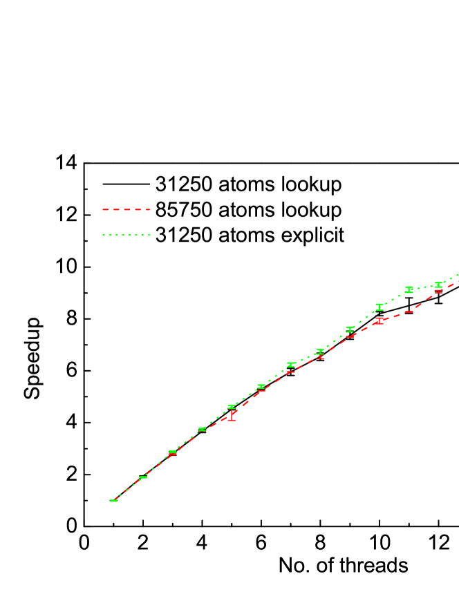
(a) Speedup comparison using two system sizes and lookup table versus direct potential evaluation. The iron potential used here is of intermediate complexity: a sum of 15 cubic splines.

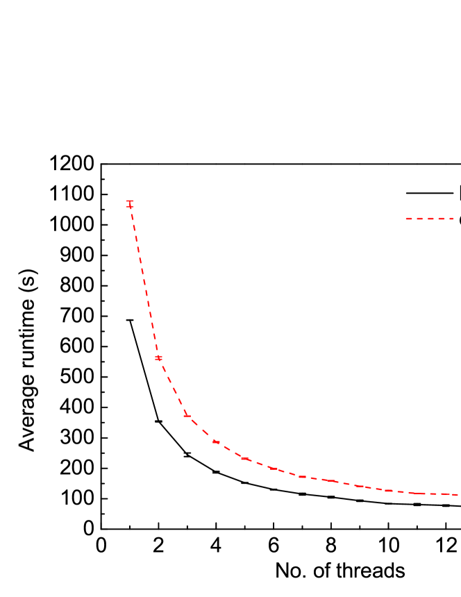
(b) Comparison in performance between using the lookup table and explicit potential evaluation. Here we use a system of 31,250 atoms.

Figure 2: Parallel performance of MOLDY when integrating a system of bcc iron for 1000 timesteps.

We evaluate the strong scaling using systems of 32k ($n$=25) and 85k ($n$=35) atoms. Fig. 2(a) shows the speedup when running using the lookup table and explicit potential calculation. We see that good scaling is achieved all the way up to our maximum of 16 threads. The explicit potential shows the best speedup; this is due to the fact that it takes longer to evaluate the force consequently increasing the parallel fraction of the code. Fig. 2(b) confirms that, in absolute terms, the lookup table method significant outperforms the explicit potential evaluation even at 16 threads.

Figure 3: The weak scaling performance of MOLDY plotted relative to the single thread runtime.

To evaluate the weak scaling we start with a system of 18k atoms (24 $\times$ 24 $\times$ 16 repeats) and increase the system size linearly with the number of threads by scaling the z-repeats accordingly. Fig. 3 shows a shallow rise in relative runtime for each additional thread caused by the serial fraction. The achieved scaling is, however, very good with a system of almost 300k atoms taking only 1.4 times as long to simulate using 16 threads as that of a 18k atom system on one thread.

Figure 4: The runtime scaling plotted as a function of the neighbour list update frequency when running on one thread. This implies that a full neighbour update takes almost twice as long as the force calculation

Finally, we evaluate the cost of neighbour list update frequency on the performance for a fixed number of threads. This may become important for simulations with a high rate of diffusion where atoms can migrate between linked-cells often. Fig. 4 shows how changing this parameter affects the runtime when using a single thread. Initially the performance cost of increasing the update frequency is fairly steep, however this quickly relaxes to linear scaling with a fairly small scale factor. From this we recommend that for simulations with little or no diffusion neighbour list updates should be kept to a minimum while for simulations with large amount of diffusion it is safe to set a conservatively high frequency without incurring a large performance penalty. It should be noted that the neighbour list update subroutine has not been parallelised and consequently a high neighbour list update frequency may adversely affect parallel speedup.

Further tests show that using a Nosé thermostat or predictor-corrector integrator in place of Verlet has little impact on the performance. The Nosé subroutine is parallelised and has been found not to affect the parallel speedup.

5.1.1 Integration error

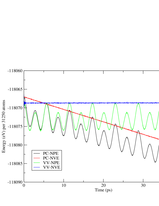
Figure 5: The total energy plotted up to 20k timesteps of 2fs when using the Verlet and predictor-corrector integration schemes. Both NVE and NPE ensembles are shown. The test system used was that from Section 5 with 31250 atoms.

To evaluate the energy drift caused by integration error we compare results from both the Verlet and predictor-corrector schemes. Fig. 5 shows the total energy plotted over 20k steps when using the test system from Section 5 comprising 31250 atoms. To obtain some drift we used a 2fs timestep, slightly larger than one would normally choose at such high temperatures. We started each simulation far from equilibrium, with atoms on their lattice sites and 1800K worth of kinetic energy. Through equipartition the temperature drops rapidly to around 900K. The coupling to the box modes is weak, and the NPE simulations oscillate in volume. In the figure, this manifests itself as an oscillation in energy as energy is transferred in and out of the fictitious modes.

Owing to its symplectic nature in the NVE ensemble, the Verlet scheme has a bounded local error and preserves the total energy globally (see e.g. [27] for a discussion of integration error from Verlet). For the NVT, NPT with Nose-Hoover thermostat no symplectic integrator is possible and energy is not conserved. For NPH ensembles Verlet is not symplectic, and since energy is exchanged between the physical system and the other terms in the Parrinello-Rahman extended Lagrangian, energy conservation should not be expected. In fact, energy is very well conserved in the extended Hamiltonian: for the physical system it oscillates about a fixed value.

Conversely the predictor-corrector exhibits a linear drift with respect to the number of timesteps in NVE ensemble, with a similar drift superimposed on the oscillations for the NPE case. In this instance this amounts to an error of $\approx$0.01% over 20k steps. While this error is small we recommend Verlet as the de facto integration scheme to be used especially in cases where thermodynamic averages are the primary quantities of interest.

6 Application Examples

6.1 Dynamic compression of copper

One of the main features of MOLDY is its very flexible approach to boundary conditions. An example where boundary conditions are important comes in simulating stamping a metal. In this experiment, the sample is subject to large uniaxial compression, inducing plastic flow into free space in the perpendicular direction.

We simulate this process for a perfect nanocrystallite of copper, with no preexisting dislocations, oriented along 100, cut along 001 and 010. The boundary conditions applied are a constant strain rate in the z-direction, with free boundaries in x and y. The process is fast, and the simulation region represents the entire sample, so we do not use a thermostat.

The constant strain rate is applied using $nsteps=1$ $strainloops=1000000$ and $STRX=0.9999995$ which applies a Parrinello-Rahman box strain to the sample every timestep. With a timestep of 1fs and a 108$\AA$ cell this is equivalent to a realistic stamping velocity of $5.4m/s$.

Snapshots of the material at various levels of strain are analysed by the BallViewer software [26]. This shows a curious sequence of events.

The material transformation occurs first by elastic strain up to the stress required for nucleation of dislocations. This is significantly higher than the yield stress of copper, implying that the barrier is the nucleation rather than the motion of the dislocations. It is lower than the nucleation stress calculated for perfect single crystal copper [28] consistent with the apparent nucleation at the surface.

Partial dislocations then travel through the material leaving steps on the surface: they leave behind them layers of material indexed as hcp on account of its local stacking[26]. Because the dislocations move on planes at an angle to the applied strain, they cross and lock, hardening the material. Slip bands are formed and the stress increases, until the macroscopic shape of the $yz$ plane changes from a square to a diamond. The orientation is now (111) (11$\overline{1}$) (1$\overline{1}$0). This change accompanies the removal of most of the stacking faults associated with the dislocations and indexed as hcp by BallViewer: the crystallite has effectively recrystallised into its new shape. This process is associated with a rise in temperature due mainly to the work done in compression. The recrystallised sample has surfaces which are now the (111) type, which have lower surface energy than the original (001) type. however the transformation does not create the lowest energy Wulff shape: the steps on the surface from the previous dislocation motion remain.

Further compression takes the system through another cycle of dislocation generation, with the diamond shape becoming increasingly stretched. This novel deformation mechanism would be strongly suppressed by periodic boundary conditions.

The stress and potential energy of the sample is monitored and shown in Fig. 7. The potential energy rises because energy is being supplied to the system from work done in compression. One can estimate the T=0 potential energy by assuming equipartition of energy between PE and KE, and evaluating PE-KE. This quantity rises steeply during the elastic phase, then drops, presumably due to reconstruction at the surface, in the second phase. In the third phase it increases slowly, this is primarily due to the increased surface area and only partly due to damage accumulating in the structure. Quenching the structure to a local potential energy minimum followed by a BallViewer analysis shows the final state to be almost perfect fcc.

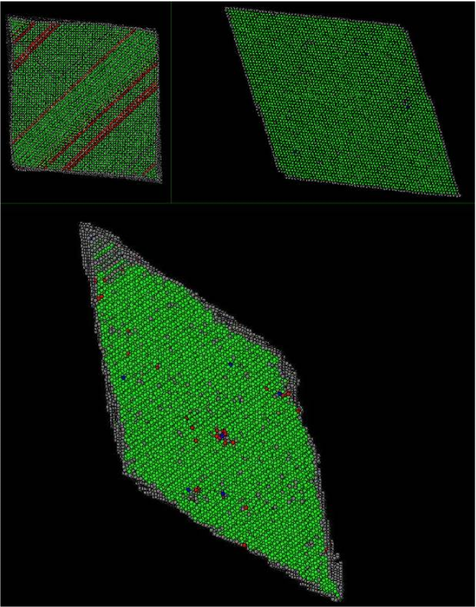
Figure 6: Top view from BallViewer of stamping simulations, all at the same scale. Green atoms are fcc, red are hcp; top left, initial yield: slip bands fringed with stacking faults; top right: reorientation transformation complete, Bottom: final state after further dislocation damage, note roughened edges.

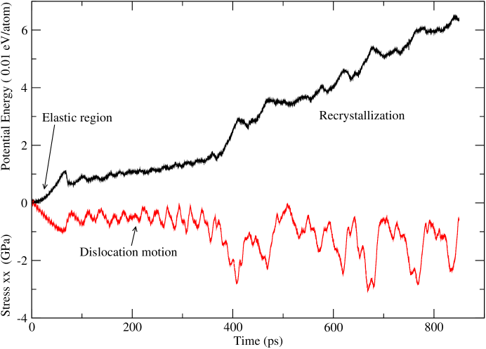
Figure 7: Evolution of stress and temperature in the constant energy constant strain rate ensemble stamping simulation. Regimes are shown corresponding to the initial elastic regime, the dislocation nucleation glide, and the reorientation/recrystallisation induced shape change of the sample.

6.2 Self-diffusion in iron

Self-diffusion, D(T), can be related to the limiting slope of the mean square displacement (MSD) of the atoms

$$D(T)=\lim_{t\to\infty}\frac{1}{6t}\langle\Delta{\bf r}(t)^{2}\rangle$$ (2)

where the term in the angle brackets is the MSD averaged over all atoms and $t$ is the simulation time. Self-diffusion for $\alpha$-iron was measured for the temperature range from 900K to 2000K using a system of 2000 atoms with a single mono-vacancy at a random site. The potential does not describe the ferro-paramagnetic transformation, so the bcc structure is stable at all these temperatures. The N-particle average of MSD against time is shown in Fig. 8. Clearly, system diffusion increases at higher temperatures, as expected. To characterise the temperature dependency of diffusion and calculate the energy of a mono-vacancy migration the data is fitted to the Arrhenius-type expression: $D(T)=D_{0}\exp(\frac{E_{f}+E_{m}}{k_{B}T})$, where $k_{B}$ is Boltzmann constant, $T$ is temperature and E_f and E_m are the energies of defect formation and migration, respectively.

The energy of vacancy migration was calculated to be E${}_{m}^{v}$ = 0.60eV with 99% confidence limits of (0.53-0.67)eV. The fit excluded temperatures $T>1800K$, where the diffusivity increases dramatically, hinting at a solid-liquid phase transition. This is in reasonable agreement with the experimental value of the melting point of iron; T_m = 1811K. In addition, the energy of formation of a vacancy was calculated using molecular statics: $E_{f}$ = 1.72eV. Both of the these values are in good agreement with previous experimental and simulation results presented in Tab. 8. The prefactor $D_{0}$ was obtained from the y-intercept in the Arrhenius graph to be $\nobreak{4.65\cdot 10^{-3}cm^{2}/s}$ with corresponding 99% confidence bounds of (2.58-8.48$\cdot 10^{-3})cm{{}^{2}}/s$. This is two orders of magnitude lower than the experimentally measured values, however in reasonable agreement with the more recent MD simulations [29, 30]. Note that due to the extrapolation to infinite temperature and the exponential sensitivity to $Q$, there are typically high errors associated with the experimentally determined values.

There is a significant stochastic error in our calculations, as D(T) was sampled at 100K intervals only, but such a large discrepancy points to an inadequacy of the potential: this may be related to the fact that the potential does not describe the transformation from bcc to fcc and back.

Table 3: Simulation and experimental results for vacancy properties of $\alpha$ iron.

Reference	$E_{m}^{v}$ (eV)	$E_{f}^{v}$ (eV)	$Q=E_{m}^{v}+E_{f}^{v}$ (eV)
	Simulation
Calder and Bacon (1993) [32]	0.91	1.83	2.74
Domain and Becquart (2002) [34]	0.65	1.9	2.55
Fu et al. (2004) [35]	0.67	2.07	2.74
Mendelev and Mishin (2009) [29]	0.60	2.18	2.78
this work	0.60	1.72	2.32
	Experiment
Schaefer et al. (1977) [37]	1.28	1.60	2.86
Vehanen et al. (1982) [38]	0.55	-	-
De Schepper et al. (1983) [39]	-	2.0	-
Romanov et al. (2006) [40]	0.73	-	-

6.3 Elastic constants in iron

We tested the shear boundary conditions by calculating the elastic constants of iron. Elastic constants vary with temperature in a way which is often well described by the semi empirical expression

$$C(T)=C(0)-\frac{s}{exp(T_{E}/T)-1}$$

where $T_{E}$ and $s$ are empirical parameters[41]. A resonant ultrasound spectroscopy study [42] suggested that the $C^{\prime}=\frac{1}{2}(C_{11}-C_{12})$ elastic modulus dropped by over 15% between 0 and 500K. Equation 6.3 then implied that it would go to zero above 2000K. We calculated the modulus from distorting a unit cell of 2000 atoms according to the C’ strain and evaluating the elastic constant from fitting the total energy at each temperature to a quadratic in the strain. This is cross-checked with the stress-strain relation. Since the potential is fitted to the zero temperature elastic moduli, good agreement at low temperature is expected. In Fig. 9 we show that although the calculated C’ softens, it does not do so as much as in the experiment. This suggests that the potential does not fully account for the physics behind the softening. The C’ elastic constant involves the same strain as the Bain transformation from bcc to fcc, which is also not correctly reproduced.

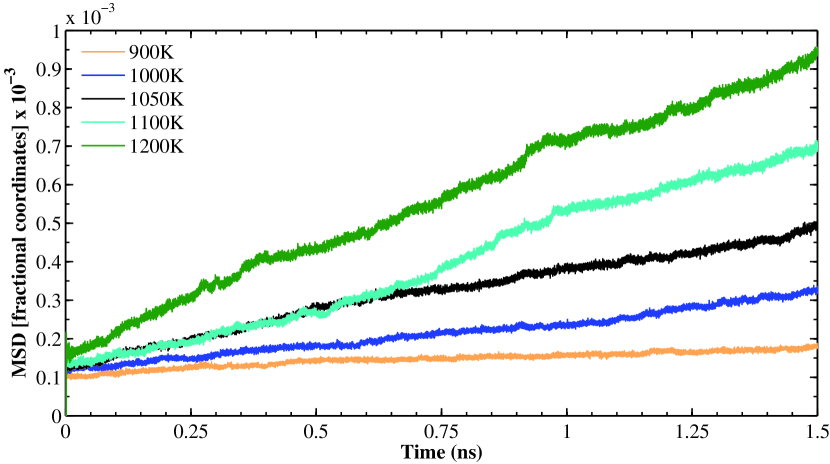
Figure 8: Calculated RMS displacements as a function of time and temperature from 2000 atom simulation with iron. Using the minimum image convention for forces, but not wraparound for atomic positions, ensures that there are no discontinuities when an atom leaves the supercell.

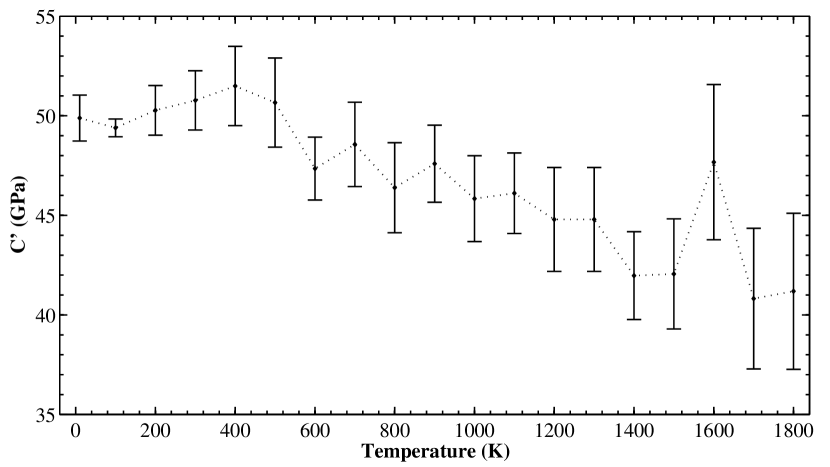
Figure 9: Variation of C’ with temperature evaluated by applying finite strains to the bcc structure and fitting a quadratic through the associated energy.

6.4 Carbon migration in iron

We also investigated the effect of carbon on diffusion in iron.

The diffusion D(T) temperature dependence and energy of migration for carbon in bcc iron was evaluated for temperature ranging up to 1800K with a 2000+1C atom cell. The energy of migration of a carbon interstitial was found to be considerably higher than that for the vacancy; $E_{m}^{C}=1.2(3)$eV$>E_{m}^{v}=0.6(1)$eV. The carbon occupies the octahedral $(1/2,0,0)$ site and the nearest adjacent site (e.g. $(1/2,1/2,0)$) lies along the (010)-type direction. However, Fig. 10 shows evidence of correlated migration along various directions (e.g. event at 2500fs) and multiple correlated motion along a (100) direction (e.g. event at 7000fs). This suggests that the martensite-type tetragonal strain field around the C can persist, enabling secondary jumps to occur [43].

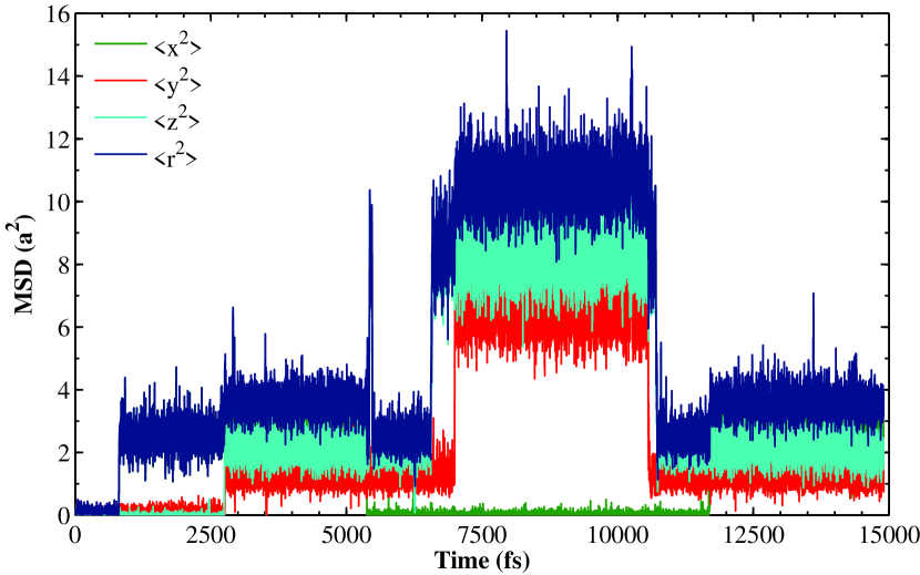
Figure 10: RMS displacement of the carbon atom through a series of jumps at 1300K.

We also investigated a 1999+1C iron system with a carbon and a vacancy. Now we find a trapping and detrapping effect: the fastest migrating species is the vacancy, followed by the vacancy-carbon complex and finally the isolated carbon (see Fig. 11). Thus the carbon acts as a weak trap for the vacancy, slowing its migration: by contrast the vacancy enhances the migration of the carbon. Even the weak vacancy trapping effect means that the overall self-diffusion rate of Fe is reduced by more than an order of magnitude due to the presence of 0.05% carbon.

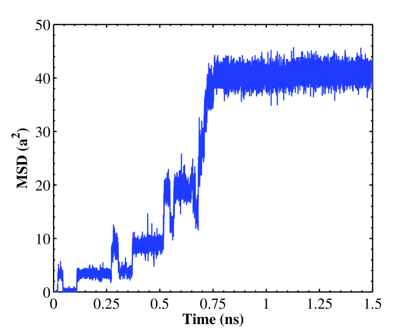
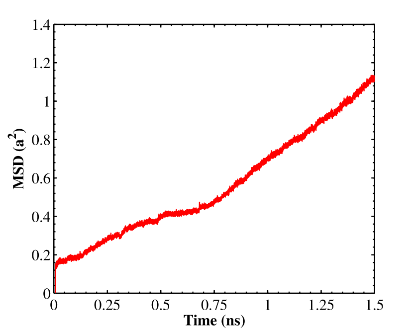
Figure 11: RMS displacement of the carbon atom through a series of jumps in a system with a vacancy at 1350K. Up to 800ps the carbon is associated with the vacancy and migrates rapidly (left panel). After 800ps carbon migration ceases, presumably due to detrapping. However migration of the vacancy is increased, as evidenced by the increased iron self-diffusion (change in slope, right panel).

7 Conclusions

We described a thoroughly updated and parallelised flexible molecular dynamics code MOLDY, which previously existed in many different versions. The program is interfaced with BallViewer, a bespoke graphics package for identifying local crystal structures and visualising MD outputs.

Furthermore, we demonstrated the parallel capabilities of MOLDY using up to 16 threads to run simulations of systems exceeding one million atoms. It was shown that the strong and weak scaling of the code provided by OpenMP parallelisation were good out to a 16-thread system.

MOLDY comes with its own test suite and we have presented applications, which illustrate some of the code features that are missing in many standard codes, such as variable boundary conditions, quenching, autocorrelation, complete stress and strain tensors. These applications show some features which are interesting in their own right, for example the crystallographic reorientation of a single nanocrystal of copper under uniaxial compression and the 100-fold reduction in iron self-diffusion due to a small amount of carbon.

8 Acknowledgements

This work was supported by the EPSRC under grant number EP/F010680/1 and by the EU-FP7 project GETMAT. We are grateful to Mark Bull for discussions on OpenMP. We also thank our codehost http://code.google.com/p/moldy/ .

References

- [1] G.J.Ackland, 1987. Non-pairwise potentials and defect modelling for transition metals. D.Phil thesis, University of Oxford.
- [2] Finnis, M. W., Harker, A. H., 1988. Moldy6 - A molecular dynamics program for simulation of pure metals. Tech. Rep. AERE R-13182, UK AEA Harwell Laboratory.
- [3] Refson, K., 2000. Moldy: A portable molecular dynamics simulation program for serial and parallel computers. Computer Physics Communications 126 (3), 310 - 329.
- [4] Parrinello, M., Rahman, A., 1981. Polymorphic transitions in single crystals: A new molecular dynamics method. Journal of Applied Physics 52 (12), 7182-7190.
- [5] Daw, M. S., Baskes, M. I., Jun 1984. Embedded-atom method: Derivation and application to impurities, surfaces, and other defects in metals. Phys. Rev. B 29 (12), 6443-6453.
- [6] Finnis, M. W., Sinclair, J. E., 1984. A simple empirical n-body potential for transition metals. Philosophical Magazine A 50 (45-55).
- [7] V. Heine, I. J. Robertson, M. C. Payne, J. N. Murrell, J. C. Phillips and D. Weaire,1991 Phil.Trans.Roy.Soc 334 393
- [8] Ackland, G. J., Finnis, M. W., Vitek, V., 1988. Validity of the second moment tight-binding model. Journal of Physics F: Metal Physics 18 (8), L153.
- [9] Dudarev S and Derlet P. (2005) Journal of Physics: Condensed Matter 17, 7097.
- [10] Ackland, G.J. Journal of Nuclear Materials 351, 1-3, 20-27 (2006)
- [11] Hepburn, D.J., Ackland, G.J., and Olsson P. Phil.Mag 89 34-36 3393 (2009)
- [12] Hepburn, D.J., Ackland, G.J., 2008. Metallic-covalent interatomic potential for carbon in Iron. Phys. Rev. B 78 (16), 165115.
- [13] Hoover, W. G., 1985. Canonical dynamics: Equilibrium phase-space distributions. Phys. Rev. A 31 (3), 1695-1697.
- [14] Nose, S., 1984. A unified formulation of the constant temperature molecular dynamics methods. The Journal of Chemical Physics 81 (1), 511-519.
- [15] Nose,S and Klein,M Mol Phys 50, 1055 (1983).
- [16] Cleveland,C.L., J.Chem.Phys. 89 4987 (1989)
- [17] Wentzcovitch R.M. Phys.Rev.B 44, 2358 (1991)
- [18] Ackland, G.J. and R. Thetford,R. Phil. Mag. A 56, 15 (1987).
- [19] Allen, M.P. and Tildesley, D.J. Computer Simulation of Liquids OUP (1987).
- [20] Ackland, G. J., Mendelev, M. I., Srolovitz, D. J., Han, S., Barashev, A. V., 2004. Development of an interatomic potential for phosphorus impurities in -Iron. Journal of Physics: Condensed Matter 16 (27), S2629.
- [21] Mendelev, M. I., Ackland, G. J., 2007. Development of an interatomic potential for the simulation of phase transformations in Zirconium. Philosophical Magazine Letters 87 (5), 349-359.
- [22] Ackland, G. J., Tichy, G., Vitek, V., Finnis, M. W., 1987. Simple n-body potentials for the noble metals and Nickel. Philosophical Magazine A 56 (6), 735-756.
- [23] Fincham D. and Heyes, D.M. , Advances in Chemical Physics. Wiley, New York (1985), p. 493
- [24] L. Verlet Phys. Rev. 159 98 (1967)
- [25] C.W. Gear, Numerical initial value problems in ordinary differential equations, Prentice Hall, EngleWood, 1973
- [26] Ackland, G. J., Jones, A. P., 2006. Applications of local crystal structure measures in experiment and simulation. Phys. Rev. B 73 (5), 054104.
- [27] Hairer, E., Lubich, C., Wanner, G., 2003. Geometric numerical integration illustrated by the Störmer/Verlet method. Acta Numerica 12, 399-450.
- [28] Tschopp, M. A., Spearot, D. E., McDowell, D. L., 2007. Atomistic simulations of homogeneous dislocation nucleation in single crystal copper. Modelling and Simulation in Materials Science and Engineering 15 (7), 693.
- [29] Mendelev, M. I., Mishin, Y., Oct 2009. Molecular dynamics study of self-diffusion in bcc Fe. Phys. Rev. B 80 (14), 144111.
- [30] Sivak, A., Romanov, V., Chernov, V., 2007. Self-point defects diffusion in bcc Iron. 13rd International Conference on Fusion Reactor Materials, 3693.
- [31] Harder, J., Bacon, D., 11 1986. Point-defect and stacking-fault properties in bodycentered-cubic metals with n-body interatomic potentials. Philosophical Magazine A - Physics Of Condensed Matter Structure Defects And Mechanical Properties 54 (5), 651-661.
- [32] Calder, A., Bacon, D., 1993. A molecular dynamics study of displacement cascades in -Iron. Journal of Nuclear Materials 207, 25 - 45.
- [33] Osetsky, Y., Mikhin, A., Serra, A., 1995. Study of copper precipitates in alpha-Iron by computer-simulation. Interatomic potentials and properties of Fe and Cu. Philosophical Magazine A - Physics Of Condensed Matter Structure Defects And Mechanical Properties 72 (2), 361-381.
- [34] Domain, C., Becquart, C. S., Dec 2001. Ab initio calculations of defects in Fe and dilute Fe-Cu alloys. Phys. Rev. B 65 (2), 024103.
- [35] Fu, C.-C., Willaime, F., Ordejón, P., Apr 2004. Stability and mobility of mono and di-interstitials in -Fe. Phys. Rev. Lett. 92 (17), 175503.
- [36] Angers, R., Claisse, F., 1968. Improvement of Kryukov and Zhukhovitskii method for measurement of diffusion. Application to self-diffusion in alpha Iron. Canadian Metallurgical Quarterly 7 (2), 73.
- [37] Schaefer, H.-E., Maier, K., Weller, M., Herlach, D., Seeger, A., Diehl, J., 1977. Vacancy formation in Iron investigated by positron annihilation in thermal equilibrium. Scripta Metallurgica 11 (9), 803 - 809.
- [38] Vehanen, A., Hautojarvi, P. , Johansson, J. , Yli-Kauppila, J. and Moser, P. , Vacancies and carbon impurities in - iron: Electron irradiation, Phys. Rev. B 25 1982, p. 762.
- [39] De Schepper, L., Segers, D., Dorikens-Vanpraet, L., Dorikens, M., Knuyt, G., Stals, L. M., Moser, P., May 1983. Positron annihilation on pure and Carbon-doped -Iron in thermal equilibrium. Phys. Rev. B 27 (9), 5257-5269.
- [40] Romanov, V. A., Sivak, A. B., Chernov, V. M., 2006. Vopr. At. Nauki Tekh., Ser.: Materialoved. I Novye Mater. 66 (129).
- [41] Varshni, Y. P., Nov 1970. Temperature dependence of the elastic constants. Phys. Rev. B 2 (10), 3952-3958.
- [42] Adams, J. J., Agosta, D. S., Leisure, R. G., Ledbetter, H., 2006. Elastic constants of monocrystal Iron from 3 to 500 K. Journal of Applied Physics 100 (11), 113530.
- [43] McLellan, R. B., Wasz, M. L., 1988. Carbon-vacancy interactions in b.c.c. Iron. Physica Status Solidi (a) 110 (2), 421-427.