High temperature thermodynamics of strongly interacting $s$-wave and $p$-wave Fermi gases in a harmonic trap

Abstract

We theoretically investigate the high-temperature thermodynamics of a strongly interacting trapped Fermi gas near either $s$-wave or $p$-wave Feshbach resonances, using a second order quantum virial expansion. The second virial coefficient is calculated based on the energy spectrum of two interacting fermions in a harmonic trap. We consider both isotropic and anisotropic harmonic potentials. For the two-fermion interaction, either $s$-wave or $p$-wave, we use a pseudopotential parametrized by a scattering length and an effective range. This turns out to be the simplest way of encoding the energy dependence of the low-energy scattering amplitude or phase shift. This treatment of the pseudopotential can be easily generalized to higher partial-wave interactions. We discuss how the second virial coefficient and thermodynamics are affected by the existence of these finite-range interaction effects. The virial expansion result for a strongly interacting $s$-wave Fermi gas has already been proved very useful. In the case of $p$-wave interactions, our results for the high-temperature equation of state are applicable to future high-precision thermodynamic measurements for a spin-polarized Fermi gas near a $p$-wave Feshbach resonance.

I Introduction

Strongly interacting fermions occur in many fields of physics, ranging from condensed matter physics to nuclear physics, astrophysics and cosmology. Recently, a new type of fermionic superfluid has been realized in ultracold atomic gases of ⁴⁰K and ⁶Li confined in a harmonic trap. In these systems the coupling strength between the fermions can be tuned precisely by an external magnetic field from weak to infinitely strong across a collisional (Feshbach) resonance. In the case of $s$-wave interactions, this has already led to the observation of a smooth crossover from a Bardeen-Cooper-Schrieffer (BCS) superfluid to a Bose-Einstein condensation (BEC). By contrast, in a Fermi system with $p$-wave interactions, a quantum phase transition is anticipated to take place instead of a smooth crossoverSadeMelo ; SadeMelo2005 ; Gurarie .

By sweeping the magnetic field, $p$-wave Feshbach resonances have recently been observed by several experimental groups ENS ; Jin ; Esslinger ; MIT ; SUT ; Zimmermann . The binding energies, lifetimes and radio-frequency spectroscopy of $p$-wave Feshbach molecules and some low-dimensional aspects of $p$-wave interactions have been investigated in these experiments. It is well known that in the dilute, low-energy limit, a two-particle $s$-wave interaction can be well characterized using a single parameter, the scattering length. However, in $p$-wave systems a new length scale - the effective range of interactions - is required, in addition to the scattering volume Idziaszek ; SadeMelo . To avoid complicated calculations in many-body systems with $p$-wave interactions, some theoretical descriptions Machida ; Machida2010 only use a constant scattering volume. This is based on the idea of a pseudopotential, which was first introduced by Huang and Yang Huang1957 . Recently, there have been several developments of the pseudopotential method for higher-partial wave interactions Stampfer2008 ; Reichenbach ; Pricoupenko ; Blume ; Stock ; Derevianko ; Bolda2002 ; Roth ; Idziaszek , using an energy-dependent scattering length. In particular, numerically exact solutions of two interacting fermions in a harmonic trap have been studied with either $s$-wave or $p$-wave couplings.

Given the interesting and unusual nature of $p$-wave interactions, in this paper we aim to investigate the high-temperature thermodynamics of a many-body, strongly interacting $p$-wave Fermi gas in a harmonic trap. The $s$-wave high-temperature thermodynamics will be also included for completeness. Our investigation is based on the virial expansion of the thermodynamic potential, which provides a natural bridge between few-body and many-body physics HO ; Liu2009 ; HU2010 ; HU2010PRA ; Ho2004 . Restricting ourselves to the leading order of the expansion, we calculate the second virial coefficient from two-fermion solutions. Consequently, we obtain the high-temperature equation of state in the strongly interacting regime, giving the energy and entropy as a function of temperature. We address in particular the role of the effective range of $p$-wave interactions in the thermodynamic state equation.

The calculation of thermodynamics in strongly interacting quantum many-body systems is always a challenge HoUniversality ; HLDUniversality ; HLDTmatrixTheory1 ; HLDTmatrixTheory2 . The only conclusive method seems to be that of $ab-initio$ quantum Monte Carlo simulation. This, however, often suffers from the sign problem for fermions. Our virial expansion approach to thermodynamics can provide an accurate benchmark for these simulations at high temperatures. Already, for $s$-wave interactions, the virial expansion has already been shown to be very useful in understanding recent thermodynamic measurements. We anticipate that our $p$-wave virial prediction will also give valuable insights and possible calibration procedures for future experiments on a Fermi gas near a $p$-wave resonance.

The calculation of the second virial coefficient requires the whole energy spectrum of the two-fermion bound states. To facilitate this calculation, we characterize the pseudopotential using two parameters, the scattering length and the effective range. This gives a simplified description for an energy-dependent scattering length. We validiate our two-parameter pseudopotential treatment by comparing the resulting spectrum with the spectrum of the full energy-dependent pseudopotential.

This paper is organized as follows. In the next section, we briefly review the derivation of the pseudopotential method for all partial-wave interactions and then introduce the two-parameter pseudopotential. The necessity of including a finite range for $p$-wave interactions is emphasized. In Sec. III, we present exact solutions for the energy spectrum of two-fermion systems with either $s$-wave or $p$-wave interactions in a harmonic trap. In Sec. IV, we calculate the second virial coefficients. Then, in Sec. V we investigate the high-temperature thermodynamics of a strongly correlated trapped Fermi gas. Finally, Sec. VI is devoted to conclusions and final remarks.

II Two-parameter pseudopotential

The first step in understanding the sophisticated physics of a quantum many-body system is to model the fundamental two-body interactions. At sufficiently low temperatures the Heisenberg uncertainty principal means that particles must spread over a distance much larger than the range of the interaction potential. In this case the details of the true interparticle potential become irrelevant and it may be modeled by a pseudopotential. The basic idea of the pseudopotential is to replace the real interaction potential by zero-range potential, which acts only at $\mathbf{r}=0$ and reproduce the same asymptotic behavior of the wave function as would occur with the real potential. The first attempt to derive a generalized pseudopotential was made by Huang and Yang Huang1957 . This has been improved by a number of authors. In this section we briefly review the derivation of the pseudopotential method Idziaszek ; Stampfer2008 .

II.1 Two-particle scattering

We consider a two-particle scattering process and assume that $V(\mathbf{r})$ is the interaction potential. The motion of the center-of-mass can be separated from the relative motion, and the Schrödinger equation in the relative coordinate can be written as

$$\frac{\hbar^{2}}{2\mu}\left(\nabla^{2}+k^{2}\right)\psi\left(\mathbf{r}\right)=V(\mathbf{r})\psi\left(\mathbf{r}\right),$$ (1)

where $k^{2}=2\mu E/\hbar^{2}$ and $\mu=m/2$ is the reduced mass, assuming identical particles apart from spin. The wavefunction has the following asymptotic behavior outside the potential range,

$$\psi_{a}\left(\mathbf{r}\right)=\sum_{l=0}^{\infty}\sum_{m=-l}^{l}C_{lm}\left[j_{l}(kr)-\tan\delta_{l}n_{l}(kr)\right]Y_{lm}(\theta,\varphi).$$ (2)

Here $Y_{lm}(\theta,\varphi)$ are spherical harmonics, $j_{l}(kr)$ and $n_{l}(kr)$ are spherical Bessel and Neumann functions respectively, and $\delta_{l}$ is the phase shift of $l$-th partial wave determined by the boundary condition.

Following Huang and Yang Huang1957 , we extend $R_{l}\left(r\right)=j_{l}(kr)-\tan\delta_{l}n_{l}(kr)$ to the vicinity of the origin at $\mathbf{r}=0$. The real interaction potential $V(\mathbf{r})$ is now replaced by the pseudopotential $V_{ps}\left(\mathbf{r}\right)$. We have

$$V_{ps}\left(\mathbf{r}\right)\psi\left(\mathbf{r}\right)=\frac{\hbar^{2}}{2\mu}\left(\nabla^{2}+k^{2}\right)\psi_{a}\left(\mathbf{r}\right)\mid_{r\rightarrow 0}.$$ (3)

The asymptotic functions of $j_{l}(kr)$ and $n_{l}(kr)$ at $r\rightarrow 0$ are given by,

$$j_{l}\left(kr\right)\simeq\frac{\left(kr\right)^{l}}{\left(2l+1\right)!!}$$

and

$$n_{l}(kr)\simeq-\frac{(2l-1)!!}{(kr)^{l+1}},$$

respectively. Thus, only $n_{l}(kr)$ is singular at small $r$. To solve Eq.(3), we use the method introduced in Idziaszek’s paper Idziaszek and obtain the pseudopotential for all partial waves as

$$V_{ps}\psi\left(\mathbf{r}\right) = \sum_{l=0}^{\infty}\sum_{m=-l}^{l}\frac{(-)^{l}16\pi^{2}}{(2l+1)!}g_{l}Y_{lm}(\partial)\delta(\mathbf{r})$$ (4)

$$\times\left[\frac{\partial^{2l+1}}{\partial r^{\prime 2l+1}}r^{\prime 2l+1}Y_{lm}^{*}(\partial^{\prime})\psi\left(\mathbf{r}^{\prime}\right)\right]_{r^{\prime}=0},$$

where

$$g_{l}=-\frac{\hbar^{2}}{2\mu}\frac{\tan\delta_{l}}{k^{2l+1}}.$$ (5)

The partial differential operator $Y_{lm}(\partial)$ is obtained from the harmonic polynomial $r^{l}Y_{lm}(\hat{r})$ by replacing the Cartesian coordinates $x_{k}$ with the partial derivatives $\partial_{x_{k}}$ MacRobert . According to Eq.(4), we can easily obtain the form of pseudopotential for any specific partial wave. Using the expression

$$\frac{4\pi}{2l+1}\sum_{m=-l}^{l}Y_{lm}(\partial)Y_{lm}^{*}(\partial^{\prime})=\sum_{k=0}^{\left[l/2\right]}c_{k}\left(\mathbf{\boldsymbol{\nabla}}\cdot\mathbf{\boldsymbol{\nabla^{\prime}}}\right)^{l-2k}\nabla^{2k}\nabla^{\prime 2k}$$ (6)

with $c_{k}=(-)^{k}(2l-2k)!/\left(2^{l}k!(l-k)!(l-2k)!\right)$, we can write the pseudopotential for $s$- and $p$-wave as

$$V_{s}=-\frac{2\pi\hbar^{2}}{\mu}\frac{\tan\delta_{0}}{k}\delta(\mathbf{r})\frac{\partial}{\partial r}r$$ (7)

and

$$V_{p}=-\frac{\pi\hbar^{2}}{\mu}\frac{\tan\delta_{1}}{k^{3}}\boldsymbol{\nabla}\delta(\mathbf{r})\frac{\partial^{3}}{\partial r^{3}}r^{3}\mathbf{\boldsymbol{\nabla^{\prime}},}$$ (8)

respectively. The symbol $\boldsymbol{\nabla}$ ($\boldsymbol{\nabla^{\prime}}$) acts only to the left (right) side of the pseudopotential.

II.2 Effective range parameters

For low energy scattering off a short range potential, it is possible to express the variation of the phase shift as

$$k^{2l+1}\cot\delta_{l}=-\frac{1}{a_{l}^{2l+1}}+\frac{1}{2}r_{l}k^{2}+O\left(k^{4}\right)$$ (9)

with only two parameters, the $l$-th partial wave scattering length $a_{l}$ and the effective range $r_{l}$ Mott1965 . If we define $R$ as the finite range of the potential, the effective range $r_{l}$ can be expressed as Madsen2002 ,

$$r_{l}\propto-\frac{2\left(2l-1\right)!!}{\left(2l-1\right)R^{2l-1}}.$$ (10)

In the low energy limit we replace the term $\tan\delta_{l}/k^{2l+1}$in Eqs. (7) and (8) by using Eq. (9). We then obtain the two-parameter pseudopotential for s-wave and p-wave interactions as

$$V_{s}=-\frac{2\pi\hbar^{2}}{\mu}\left(-a_{0}^{-1}+\frac{1}{2}r_{0}k^{2}\right)^{-1}\delta(\mathbf{r})\frac{\partial}{\partial r}r$$ (11)

and

$$V_{p}=-\frac{\pi\hbar^{2}}{\mu}\left(-a_{1}^{-3}+\frac{1}{2}r_{1}k^{2}\right)^{-1}\boldsymbol{\nabla}\delta(\mathbf{r})\frac{\partial^{3}}{\partial r^{3}}r^{3}\boldsymbol{\nabla^{\prime},}$$ (12)

respectively.

Neglecting the term $r_{0}k^{2}/2$ in Eq. (11), the two-parameter s-wave pseudopotential will result in the famous Huang-Yang $s$-wave zero-range pseudopotential,

$$\frac{2\pi\hbar^{2}a_{0}}{\mu}\delta(\mathbf{r})\frac{\partial}{\partial r}r.$$ (13)

However, as we know that using the single parameter, $s$-wave scattering length, pseudopotential is not always a good approximation in a high-density or tightly trapped system, as shown by by Blume and Bolda et al. Blume2002 ; Bolda2002 . In such cases, the next term in the expansion needs to be included.

For higher partial-wave interactions, for example $p$-wave scattering, the zero-range pseudopotential fails to describe the scattering even in the low-energy limit Idziaszek . This can be understood by the zero-range approximation constraint condition $\left|1/a_{l}^{2l+1}\right|\gg r_{l}k^{2}$ or, using the result of the effective range equation (10),

$$\left|ka_{l}\right|\ll\left(kR\right)^{\frac{2l-1}{2l+1}}.$$ (14)

Writing this out explicitly in the two cases of s-wave and p-wave interactions, we see that this implies:

$$\left|ka_{0}\right| \ll 1/\left(kR\right)\,\,\,\,\,\,s-wave\,case$$

$$\left|ka_{1}\right| \ll \left(kR\right)^{1/3}\,\,\,\,\,\,p-wave\,case$$ (15)

This means that zero-range approximation is useful for short range interactions with $kR\rightarrow 0$ in the s-wave case, since the dimensionless interaction range $\left(kR\right)$ can always be made arbitrarily small in order to satisfy the above inequality, even if $\left|ka_{l}\right|\gg 1$. In practise, this is achieved at low density and ultralow temperatures, ie, by reducing $k$. However, this limit cannot be used in the strongly interacting p-wave regime with $\left|ka_{l}\right|\gg 1$. For these higher partial-wave terms, the right-hand side will decrease as $kR\rightarrow 0$, meaning that a finite range correction is required in order to reach strongly interacting regime.

It should be noted that for any given values of range and scattering length, one can always reach the zero-range regime at sufficient dilution, as expected. In the s-wave case one has to satisfy $k^{2}\ll(R\left|a_{0}\right|)^{-1}$ . It is clearly possible to reach a regime where simultaneously $kR\ll 1$ and $\left|ka_{0}\right|\gg 1$, provided $k$ is small and $\left|a_{0}\right|$ is very large. However, in the p-wave case the inequality becomes

$$k^{2}\ll R/\left|a_{1}\right|^{3}\,.$$

The problem is that if $R\ll\left|a_{1}\right|$, which is the case near a Feshbach resonance, then satisfying this p-wave inequality requires low enough densities such that $\left|ka_{1}\right|\ll\left|kR\right|^{1/3}$ . At such low densities one is no longer in the strongly interacting regime, since this inequality is only satisfied if $\left|ka_{1}\right|\ll 1$. Finally, it should be pointed out that the pseudopotential is not a Hermitian operator. However, away from the unphysical region of the origin, we have a well-defined scattering problem.

III two fermions in a harmonic trap

The two-body problem with $s$-wave and $p$-wave interactionsSuzuki2009 in a three-dimensional harmonic trap was solved using a zero-range pseudopotential by Busch and Idziaszek et al Busch1998 ; Idziaszek2006 . Here we use the two-parameter pseudopotential given above. In an axially symmetric harmonic trap, the motion of the center of mass can be separated from the relative motion, and the relative Hamiltonian is given by

$$\left[-\frac{\hbar^{2}}{2\mu}\nabla^{2}+\frac{1}{2}\mu\omega^{2}\left(\eta^{2}\boldsymbol{\rho}^{2}+\mathbf{z}^{2}\right)+V_{ps}\right]\psi_{rel}=E_{rel}\psi_{rel},$$ (16)

where $\boldsymbol{\rho}=\boldsymbol{\rho}_{1}-\boldsymbol{\rho}_{2}$, $\mathbf{z}=\mathbf{z}_{1}-\mathbf{z}_{2}$ and $\mathbf{r}=\mathbf{r}_{1}-\mathbf{r}_{2}$ are the relative coordinates, $\mu$ is the reduced mass, $\omega$ is the transverse frequency of the trap, $\eta=\omega_{\rho}/\omega$, and $V_{ps}(\mathbf{r})$ is the two-parameter pseudopotential. To solve Eq. (16), we expand the relative wavefunction $\psi_{rel}\left(\mathbf{r}\right)$ into the complete set of the eigenfunctions of three-dimensional harmonic oscillator,

$$\psi_{rel}\left(\mathbf{r}\right)=\sum_{n_{1},n_{2},n_{3}}C_{n_{1}n_{2}n_{3}}\varphi_{n_{1,}n_{2}n_{3}}\mathbf{\left(r\right),}$$ (17)

where $\varphi_{n_{1}n_{2}n_{3}}(\mathbf{r})=\phi_{n_{1}}(\eta x/d)\phi_{n_{2}}(\eta y/d)\phi_{n_{3}}(z/d)$, $d=\sqrt{\hbar/\mu\omega}$ is the oscillator length in the transverse direction and $\phi_{n}(\xi)$ can be expressed by a Hermite polynomial as

$$\phi_{n}(\xi)=\sqrt{\frac{1}{\sqrt{\pi}2^{n}n!}}e^{-\xi^{2}/2}H_{n}\left(\xi\right).$$

Considering an isotropic harmonic trap, $\varphi_{n_{1}n_{2}n_{3}}(\mathbf{r})$ can be replaced by the spherical harmonic function $Y_{lm}\left(\theta,\varphi\right)$ and the function $R_{nl}\left(r\right)$, written as

$$\varphi_{nlm}\left(\mathbf{r}\right)=R_{nl}\left(r\right)Y_{lm}\left(\theta,\varphi\right).$$ (18)

Using the generalized Laguerre polynomials $L_{n}^{(l+1/2)}$, we can express the function $R_{nl}$ as $R_{nl}=N_{nl}\left(r/d\right)^{l}exp\left(-r^{2}/2d^{2}\right)L_{n}^{(l+1/2)}\left(r^{2}/d^{2}\right)$. Here $N_{nl}$ is the normalization coefficient.

III.1 $s$-wave interaction in a 3D isotropic trap

As a preliminary calculation, we consider two fermions with unlike spins interacting via $s$-wave interactions in a 3D isotropic harmonic trap, with $\eta=\omega_{z}/\omega=1$. The relative wavefunction can be written in the form of Eq. (18). For $s$-wave interactions, we only need to keep $l=0$ in Eq. (18) as $l\neq 0$ modes are not affected by the interactions. The relative wavefunction of interest can then be written as

$$\psi_{rel}\left(\mathbf{r}\right)=\sum_{n}C_{n}\varphi_{n}\mathbf{\left(r\right)},$$ (19)

where $\varphi_{n}\left(\mathbf{r}\right)=R_{n0}\left(r\right)Y_{00}\left(\theta,\varphi\right)$. We insert this relative wavefunction into Eq. (16). Following the derivation by Busch et al. Busch1998 the energy level $E_{rel}$ should satisfy the following expression,

$$\frac{2\pi\hbar\omega}{d}\left[\frac{\partial}{\partial r}\left(r\sum_{n}\frac{\varphi_{n}^{*}\left(0\right)\varphi_{n}\left(\mathbf{r}\right)}{E_{n}-E_{rel}}\right)\right]_{r\rightarrow 0}=-\frac{1}{a_{0}}+\frac{1}{2}r_{0}k^{2},$$ (20)

where $E_{n}=\left(2n+3/2\right)\hbar\omega$ and we have defined $E_{rel}=\left(2\nu+3/2\right)\hbar\omega$. By using $R_{n0}=N_{n0}exp\left(-r^{2}/2d^{2}\right)L_{n}^{1/2}\left(r^{2}/d^{2}\right)$ and the relationship between the Laguerre polynomials $L_{n}^{1/2}\left(x\right)$ and the confluent hypergeometric function $U,$

$$\sum_{n=0}^{\infty}\frac{L_{n}^{1/2}\left(x\right)}{n-\nu}=\Gamma\left(-\nu\right)U\left(-\nu,\frac{3}{2},x\right),$$ (21)

Eq. (20) can be simplified to

$$\frac{1}{\sqrt{\pi}}\Gamma\left(-\nu\right)U\left(-\nu,\frac{3}{2},\frac{r^{2}}{d^{2}}\right)=-\frac{d}{a_{0}}+\frac{d}{2}r_{0}k^{2},$$ (22)

where $\Gamma\left(x\right)$ is the Gamma function. By examining the short-range behavior of the confluent hypergeometric function,

$$\Gamma\left(-\nu\right)U\left(-\nu,\frac{3}{2},r^{2}\right)=-\sqrt{\pi}\left[\frac{2\Gamma\left(-\nu\right)}{\Gamma\left(-\nu-1/2\right)}-\frac{1}{r}+O\left(r\right)\right],$$ (23)

and taking the approximation $k^{2}=2\mu E_{rel}/\hbar^{2}$, we obtain a secular equation for the relative energy levels:

$$\frac{2\Gamma\left(-\nu\right)}{\Gamma\left(-\nu-1/2\right)}=\frac{d}{a_{0}}-\frac{r_{0}}{d}\cdot\left(2\nu+\frac{3}{2}\right).$$ (24)

Here the second term on the right hand side of Eq. (24) shows the effects of the finite-range interaction potential. Taking a zero range limit, with $r_{0}=0$, Eq. (24) gives Busch’s earlier result Busch1998 . The relative wave functions can be found to be:

$$\psi_{rel}\left(\mathbf{r}\right)\propto exp\left(-\frac{r^{2}}{2d^{2}}\right)\Gamma\left(-\nu\right)U\left(-\nu,\frac{3}{2},\frac{r^{2}}{d^{2}}\right).$$ (25)

In Fig. 1, we give the energy spectrum of two fermions with $s$-wave interactions as a function of the dimensionless interaction strength $d/a_{0}$. Here we consider two cases:

(i)

zero-range limit (red dotted line) and

(ii)

$r_{0}/d=2R/d=0.1$ (blue solid line).

It is easy to see that, except for the lowest bound state, the two lines differ slightly. The most significant difference appears around the unitarity limit with $a_{0}\rightarrow\pm\infty$. Thus, the zero-range approximation appear to be sound as far as the lowest bound state is concerned. Therefore, the scattering length $a_{0}$ can be used to characterize the low-energy$s$-wave scattering, provided that the finite range of the interaction potential is smaller than the characteristic length of the harmonic trap, $d$.

In the limiting case of zero scattering length, we find that the asymptotic behavior of the energy spectrum for the $n$-th level can be described by,

$$\frac{E_{rel}}{\hbar\omega}=2n+\frac{3}{2}+\frac{4\Gamma\left(n+3/2\right)}{\pi\Gamma\left(n+1\right)\left[d/a_{0}-\left(2n+3/2\right)r_{0}/d\right]},$$

where $n=0,1,2,\ldots$ is a non-negative integer.

Near the unitarity limit, the asymptotic behavior of the energy spectrum for the $n$-th level can be written as

$$\frac{E_{rel}}{\hbar\omega}=2n+\frac{1}{2}+2q,$$ (26)

where

$$q=-\frac{\Gamma\left(n+1/2\right)d}{2\pi\Gamma\left(n+1\right)a_{0}}+\frac{\left(2n+1/2\right)\Gamma\left(n+1/2\right)r_{0}}{2\pi\Gamma\left(n+1\right)d}.$$ (27)

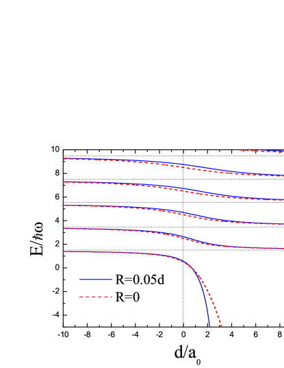
Figure 1: (Color online) The energy spectrum of two fermions with $s$-wave interactions in a 3D isotropic harmonic trap, as a function of the dimensionless interaction parameter $d/a_{0}$ at two different effective ranges of interactions: $r_{0}/d=0$ (red dotted lines) and $r_{0}/d=0.1$ (blue solid lines).

III.2 $p$-wave interactions in a 3D isotropic trap

Let us now consider two fermions with $p$-wave interactions in a 3D isotropic harmonic trap. We keep only the $l=1$ term in Eq. (18), since other $l\neq 1$ channels are not affected by $p$-wave interactions. We may then write the relative wavefunction,

$$\psi_{rel}\left(\mathbf{r}\right)=\sum_{nm}C_{n1m}R_{n1}\left(r\right)Y_{1m}\left(\theta,\varphi\right).$$ (28)

Substituting Eq. (28) into Eq. (16), we obtain

$$\sum_{nm}\frac{\left\{\boldsymbol{\nabla}\varphi_{n1m}^{*}\left(\mathbf{r}\right)\left(\partial^{3}/\partial r^{3}\right)\left[r^{3}\boldsymbol{\nabla}\varphi_{n1m}\left(\mathbf{r}\right)\right]\right\}{}_{r\rightarrow 0}}{E_{nl}-E_{rel}}$$

$$=\frac{\mu}{\pi\hbar^{2}}\left(-a_{1}^{-3}+\frac{1}{2}r_{1}k^{2}\right)^{-1},$$ (29)

where $E_{nl}=\left(2n+1+3/2\right)\hbar\omega$ is the non-interacting relative energy and we have written the interacting energy eigenvalue as $E_{rel}=\left(2\nu+5/2\right)\hbar\omega$. Using $\sum_{m}Y_{lm}^{*}\left(\theta,\varphi\right)Y_{lm}\left(\theta,\varphi\right)=\left(2l+1\right)/4\pi$ and $R_{n1}=N_{n1}\left(r/d\right)exp\left(-r^{2}/2d^{2}\right)L_{n}^{3/2}\left(r^{2}/d^{2}\right)$, we obtain

$$\left\{\frac{\partial^{3}}{\partial r^{3}}r^{2}\left[r\exp\left(-\frac{r^{2}}{2d^{2}}\right)\sum_{n}\frac{L_{n}^{3/2}\left(r^{2}/d^{2}\right)}{\left(2n+5/2\right)\hbar\omega-E_{rel}}\right]\right\}_{r\rightarrow 0}$$

$$=\frac{d^{5}\sqrt{\pi}\mu}{2\hbar^{2}}\left(-a_{1}^{-3}+\frac{1}{2}r_{1}k^{2}\right)^{-1}.$$ (30)

Using the identity between the Laguerre polynomials $L_{n}^{3/2}\left(r^{2}\right)$ and the confluent hypergeometric function $U$,

$$\sum_{n}\frac{L_{n}^{3/2}\left(r^{2}/d^{2}\right)}{\left(2n+5/2\right)\hbar\omega-E_{rel}}=\frac{1}{2\hbar\omega}\Gamma\left(-\nu\right)U\left(-\nu,\frac{5}{2},\frac{r^{2}}{d^{2}}\right),$$ (31)

and the asymptotic behavior of the confluent hypergeometeric function at $r\rightarrow 0$,

$$\frac{1}{\pi}\Gamma\left(-\nu\right)U\left(-\nu,\frac{5}{2},r^{2}\right)=-\frac{r^{-3}}{\Gamma\left(-1/2\right)}\\ -\frac{2\nu+3}{r\Gamma\left(-1/2\right)}+\frac{\Gamma\left(-\nu\right)}{\Gamma\left(-\nu-3/2\right)\Gamma\left(5/2\right)},$$ (32)

the eigenvalue equation Eq. (30) leads to

$$\frac{\Gamma\left(-\nu+1/2\right)}{\Gamma\left(-\nu-1\right)}=-\frac{1}{8}\cdot\left(\frac{d}{a_{1}}\right)^{3}+\frac{1}{8}\cdot\left(dr_{1}\right)\cdot\left(2\nu+\frac{3}{2}\right).$$ (33)

Here we take the same approximation $k^{2}=2\mu E_{rel}/\hbar^{2}$ as in the $s$-wave case. The corresponding eigenfunctions have the form,

$$\psi_{rel}\left(\mathbf{r}\right) \propto \left(\frac{r}{d}\right)exp\left(-\frac{r^{2}}{2d^{2}}\right)\times$$ (35)

$$\Gamma\left(-\nu+\frac{1}{2}\right)U\left(-\nu+\frac{1}{2},\frac{5}{2},\frac{r^{2}}{d^{2}}\right)Y_{1m}.$$

In Fig. 2, we give the energy spectrum of two fermions with $p$-wave interactions as a function of the dimensionless inverse scattering volume $d^{3}/a_{1}^{3}$. The red dotted line and blue solid line correspond to a zero effective range $r_{1}d=0$ and a finite effective range $r_{1}d=-40$, respectively. The value of $r_{1}d=-40$ is calculated from the finite range of interaction potentials, $R=0.05d$, using $R=-2/r_{1}$. Unlike the $s$-wave case, near the unitarity limit, a small finite-range parameter in the interaction potential can induce a significant change of the energy spectrum, implying that the use of zero-range pseudopotential is not justified for $p$-wave interactions in the unitarity limit, as expected.

This can be understood using Eq. (14). For $p$-wave interactions, the zero-range approximation is valid only if $\left|ka_{1}\right|\ll\left(kR\right)^{1/3}$. For a small value of $R$ and a large scattering length $a_{1}$, the wavelength or the collision energy therefore should be extremely small in order to satisfy this constraint. As explained in Section II, this limit can only be achieved if $\left|ka_{1}\right|\ll 1$ , which is no longer in the strongly-interacting regime. In contrast, for $s$-wave interactions, we only require that $\left|ka_{0}\right|\ll\left(kR\right)^{-1}$, which can generally be satisfied at low dilutions near a Feshbach resonance. We have checked our two-parameter pseudopotential method, by comparing its energy spectrum with that predicted by a more complex energy-dependent pseudopotential approach Idziaszek . For typical parameters corresponding to the experimental condition for ⁴⁰K fermions, we find an excellent agreement between these two pseudopotentials.

In the non-interacting limit of zero scattering length, we find that the following asymptotic form for the $n$-th energy level,

$$\frac{E_{rel}}{\hbar\omega}=2n+\frac{5}{2}+\frac{8\Gamma\left(n+5/2\right)}{\pi\Gamma\left(n+1\right)\left(d^{3}/2a_{1}^{3}-r_{1}d\left(n+5/4\right)\right)}.$$ (36)

In the zero range limit, Eq. (36) implies that the interacting energy spectrum differs mostly from the non-interacting spectrum at the resonance position $a_{1}\rightarrow\infty$. However, the existence of a finite range of interactions will shift the position to the BCS side, which is determined by the condition, $d^{3}/(2a_{1}^{3})-r_{1}d\left(n+5/4\right)=0$.

Near the unitarity limit, the lowest energy level is approximately zero. The asymptotic value of energy spectrum for the $n$-th level is given by,

$$\frac{E_{rel}}{\hbar\omega}=2n+\frac{5}{2}+2q,$$ (37)

where

$$q=\frac{-\Gamma\left(n+\frac{5}{2}\right)}{\pi\left(n+\frac{5}{4}\right)\Gamma\left(n+1\right)}\left(\frac{4}{r_{1}d}+\frac{2d}{a_{1}^{3}r_{1}^{2}\left(n+5/4\right)}\right).$$ (38)

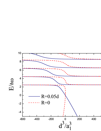
Figure 2: (Color online) The energy spectrum of two fermions with $p$-wave interactions in a 3D isotropic harmonic trap, as a function of the dimensionless inverse scattering volume $d^{3}/a_{1}^{3}$ at two different effective ranges: $r_{1}d=0$ (red dotted lines) and $r_{1}d=-40$ (blue solid lines).

III.3 $p$-wave interactions and 3D anisotropic traps

Let us now turn to the case of two fermions with $p$-wave interactions in an anisotropic 3D harmonic trap $\mu\omega^{2}\left(\eta^{2}\boldsymbol{\rho}^{2}+\mathbf{z}^{2}\right)/2$. We have to take the general form Eq. (17) for the relative wavefunction $\psi_{rel}\left(\mathbf{r}\right)$. By substituting Eq. (17) into Eq.(16), we follow the derivation for $s$-wave interactions given by Busch et al. Busch1998 . This leads to the following expression for the eigenvalues $E_{rel}$,

$$\sum_{n_{1}^{\prime}n_{2}^{\prime}n_{3}^{\prime}}C_{n_{1}^{\prime}n_{2}^{\prime}n_{3}^{\prime}}\frac{\left\{\boldsymbol{\nabla}\varphi_{n^{\prime}_{1}n^{\prime}_{2}n^{\prime}_{3}}^{*}\left(\partial^{3}/\partial r^{3}\right)\left[r^{3}\boldsymbol{\nabla}\varphi_{n^{\prime}_{1}n^{\prime}_{2}n^{\prime}_{3}}\mathbf{\left(r\right)}\right]\right\}{}_{r\rightarrow 0}}{\left(E_{n^{\prime}_{1}n^{\prime}_{2}n^{\prime}_{3}}-E_{rel}\right)C_{n_{1}n_{2}n_{3}}}$$

$$=\frac{\mu}{\pi\hbar^{2}}\left(-a_{1}^{-3}+\frac{1}{2}r_{1}k^{2}\right),$$ (39)

where $C_{n_{1}n_{2}n_{3}}=\left[\nabla\varphi_{n^{\prime}_{1,}n^{\prime}_{2}n^{\prime}_{3}}^{*}\mathbf{\left(r\right)}\right]_{r\rightarrow 0}$ and the non-interacting energy spectrum is given by $E_{n_{1}n_{2}n_{3}}=\left(n_{1}+1/2\right)\hbar\omega_{x}+\left(n_{2}+1/2\right)\hbar\omega_{y}+\left(n_{3}+1/2\right)\hbar\omega_{z}$. To proceed, we re-write the summation in the above equation by using the identity,

$$\frac{1}{E_{n}-E}=\int_{0}^{\infty}dte^{-t\left(E_{n}-E\right)}$$

for $E<E_{0}=\hbar\left(\omega_{x}+\omega_{y}+\omega_{z}\right)/2$, and use the relation satisfied by the Hermite polynomial,

$$\sum_{k=0}^{\infty}\frac{t^{k}}{2^{k}k!}H_{k}(x)H_{k}(y)=\frac{e^{\left(2txy-t^{2}x^{2}-t^{2}y^{2}\right)/\left(1-t^{2}\right)}}{\sqrt{1-t^{2}}}.$$

As a result, the left-hand side of Eq. (39) can be expressed by using the function ($l=x,y,z$ )

$$H_{l}\left(\epsilon,\mathbf{r}\right)=\int_{0}^{\infty}dt\frac{e^{t\left(\epsilon-\eta_{l}\right)}}{1-e^{-2\eta_{l}t}}\prod_{i=1}^{3}\frac{\exp\left[-\eta_{i}\frac{x_{i}^{2}e^{-2\eta_{i}t}}{1-e^{-2\eta_{i}t}}\right]}{\sqrt{1-e^{-2\eta_{i}t}}}.$$

At $r\rightarrow 0$, the asymptotic behavior of $H_{l}\left(\epsilon=\left(E-E_{0}\right)/\hbar\omega,\mathbf{r}\right)$ is given by,

$$H_{l}\left(\epsilon,\mathbf{r}\right)=F_{l}\left(\epsilon,\mathbf{r}\right)+\frac{\sqrt{\pi}}{4\eta\eta_{l}r^{3}}+\frac{\left(2\epsilon+2\eta+1\right)\sqrt{\pi}}{8\eta\eta_{l}r},$$

where

$$F_{l}\left(\epsilon,\mathbf{r}\right) = \int_{0}^{\infty}dt\left\{\frac{e^{t\left(\epsilon-\eta_{l}\right)}}{1-e^{-2\eta_{l}t}}\prod_{i=1}^{3}\frac{\exp\left[-\eta_{i}\frac{x_{i}^{2}e^{-2\eta_{i}t}}{1-e^{-2\eta_{i}t}}\right]}{\sqrt{1-e^{-2\eta_{i}t}}}-\right.$$ (40)

$$\left.-\left[\frac{e^{-r^{2}/2t}}{4\sqrt{2}\eta\eta_{l}}\left(\frac{1}{t^{5/2}}+\frac{2\epsilon+2\eta+1}{2t^{3/2}}\right)\right]\right\}$$

and $\eta_{x}=\eta_{y}=\eta$ and $\eta_{z}=1$. After a straightforward but lengthy calculation, we find that

$$\frac{12\eta\eta_{l}}{\sqrt{\pi}}F_{l}\left(\frac{E_{rel}-E_{0}}{\hbar\omega},0\right)=-\left(\frac{d}{a_{1}}\right)^{3}+r_{1}d\frac{E_{rel}}{\hbar\omega}.$$ (41)

Here we take the same approximation $k^{2}=2\mu E_{rel}/\hbar^{2}$ as before and $F_{l}\left(E_{rel},0\right)\equiv F_{l}\left(E_{rel},\mathbf{r}=0\right)$. In an axially symmetric trap, we may use the good quantum number of projected angular momentum $m$ to label the energy levels. The secular equations for $m=\pm 1$ and for $m=0$ are, respectively Idziaszek ,

$$\frac{12\eta^{2}}{\sqrt{\pi}}F_{x}\left(\frac{E_{rel}-E_{0}}{\hbar\omega},0\right)=-\frac{d^{3}}{a_{1}^{3}}+r_{1}d\cdot\frac{E_{rel}}{\hbar\omega}$$ (42)

and

$$\frac{12\eta}{\sqrt{\pi}}F_{z}\left(\frac{E_{rel}-E_{0}}{\hbar\omega},0\right)=-\frac{d^{3}}{a_{1}^{3}}+r_{1}d\cdot\frac{E_{rel}}{\hbar\omega}.$$ (43)

To calculate the eigenvalue, for $E_{rel}<E_{0}$ we use the integral equation Eq. (40), while for $E_{rel}>E_{0}$ we use the recurrence relations Idziaszek ,

$$F_{x}\left(\epsilon+2\eta\right)-2F_{x}\left(\epsilon\right)+F_{x}\left(\epsilon-2\eta\right)$$

$$=\frac{\sqrt{\pi}}{2}\cdot\frac{\Gamma\left(-\eta/2-\epsilon/2\right)}{\Gamma\left(1/2-\eta/2-\epsilon/2\right)}$$ (44)

and

$$F_{z}\left(\epsilon+2\eta,0\right)-F_{z}\left(\epsilon,0\right)=-\sqrt{\pi}\cdot\frac{\Gamma\left(1/2-\eta-\epsilon/2\right)}{\Gamma\left(-\eta-\epsilon/2\right)}$$ (45)

where $\epsilon=\left(E-E_{0}\right)/\hbar\omega$.

In Figs. 3 and 4, we show the energy spectrum of two interacting fermions with $p$-wave interactions, as a function of the dimensionless inverse scattering volume $d^{3}/a_{1}^{3}$ at an effective range $r_{1}d=-40$, in a cigar-shaped trap ($\eta=5$) and in a pancake-shaped trap ($\eta=0.2$), respectively. These plots are similar to the energy spectrum of two fermions in an isotropic trap. However, due to the trap anisotropy, the degeneracy for different projected angular momentum $m$ is removed.

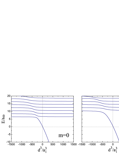
Figure 3: (Color online) The energy spectrum of two fermions with $p$-wave interactions in a 3D anisotropic harmonic trap, as a function of the dimensionless inverse scattering volume $d^{3}/a_{1}^{3}$ at $\eta=\omega_{\rho}/\omega=5$ and the effective range $r_{1}d=-40$.

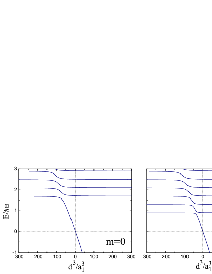
Figure 4: (Color online) The energy spectrum of two fermions with $p$-wave interactions, as in Fig. 3, but with $\eta=\omega_{\rho}/\omega=0.2$.

IV Virial Expansion of strongly correlated fermions

The knowledge of few-particle exact solutions provides a useful input for investigating the high-temperature behavior and many-body physics of a strongly correlated quantum gas. This is provided by the quantum virial expansion technique HO ; Liu2009 ; HU2010 ; Liu2010 . The essential idea of the quantum virial expansion is that at high temperatures the chemical potential $\mu$ is negative and the fugacity $z\equiv\exp(\mu/k_{B}T)\equiv\exp(\beta\mu)\ll 1$ is a well-defined small parameter. We can therefore expand the thermodynamic potential $\Omega$ of a quantum system in powers of the fugacity, regardless of the strength of the interactions. In general we may write,

$$\Omega=-k_{B}TQ_{1}\left(z+b_{2}z^{2}+\cdots+b_{n}z^{n}+\cdots\right)$$ (46)

where $Q_{n}$ is the partition function of a cluster that contain $n$ particles

$$Q_{n}=\mathrm{Tr}_{n}\left[exp\left(-\mathcal{H}/k_{B}T\right)\right].$$ (47)

The trace $Tr_{n}$ takes into account all the $n$-particle states with a proper symmetry. The $n$-th virial coefficient $b_{n}$ has the form:

$$b_{2} = \frac{Q_{2}-Q_{1}^{2}/2}{Q_{1}}$$ (48)

$$b_{3} = \frac{Q_{3}-Q_{1}Q_{2}+Q_{1}^{3}/3}{Q_{1}}$$

$$\vdots$$

All the other thermodynamic properties can then be derived from $\Omega$ via the standard thermodynamic relations.

It is convenient to focus on the effect of interactions on the virial coefficients. To this end, we consider the differences $\Delta Q_{n}=Q_{n}-Q_{n}^{(1)}$ and $\Delta b_{n}=b_{n}-b_{n}^{(1)}$, where the superscript “$1$” denotes an ideal, non-interacting system having the same fugacity. Accordingly, we rewrite the thermodynamic potential in the form,

$$\Omega=\Omega^{(1)}-k_{B}TQ_{1}\left[\Delta b_{2}z^{2}+\cdots+\Delta b_{n}z^{n}+\cdots\right],$$ (50)

where $\Omega^{(1)}$ is the non-interacting thermodynamic potential and

$$\Delta b_{2} = \Delta Q_{2}/Q_{1}$$ (51)

$$\Delta b_{3} = \Delta Q_{3}/Q_{1}-\Delta Q_{2}$$

$$\vdots$$

We now describe how to calculate the non-interacting thermodynamic potential $\Omega^{(1)}$ and the virial coefficients $\Delta b_{n}$.

IV.1 Ideal thermodynamic potential

The non-interacting virial coefficients can be determined straightforwardly from the non-interacting thermodynamic potential. For a harmonically trapped Fermi gas, the non-interacting thermodynamic potential in the semiclassical limit (i.e., neglecting the discreteness of the spectrum) is,

$$\Omega^{(1)}=-\frac{2\left(k_{B}T\right)^{4}}{\left(\hbar\bar{\omega}\right)^{3}}\frac{1}{2}\int\limits_{0}^{\infty}t^{2}\ln\left(1+ze^{-t}\right)dt,$$ (53)

where $Q_{1}=2\left(k_{B}T\right)^{3}/\left(\hbar\bar{\omega}\right)^{3}$ and $\hbar\bar{\omega}=\eta^{2/3}\hbar\omega$. Taylor-expanding the non-interacting thermodynamic potential in powers of $z$ gives rise to

$$b_{n}^{(1)}=\frac{\left(-1\right)^{n+1}}{n^{4}}.$$ (54)

IV.2 Second virial coefficient in a harmonic trap

To calculate the second virial coefficient of a trapped interacting Fermi gas, we use $\tilde{\omega}=\hbar\omega/k_{B}T\ll 1$ to characterize the intrinsic length scale relative to the trap. To obtain $\Delta b_{2}$, we consider separately $\Delta Q_{2}$ and $Q_{1}$. The single-particle partition function $Q_{1}$ can be determined by the single-particle spectrum of a 3D harmonic oscillator or alternatively can be derived from the well-known ideal thermodynamic potential. We find

$$Q_{1}\cong 2\left(k_{B}T\right)^{3}/\left(\hbar\bar{\omega}\right)^{3}\,.$$ (55)

The prefactor of two accounts for the two possible spin states of a single fermion. In the calculation of $\Delta Q_{2}$, it is easy to see that the summation over the center-of-mass energy level gives exactly $Q_{1}/2$. Thus, the second virial coefficient is determined entirely by the relative energy spectrum $E_{rel}$ and we find that,

$$\Delta b_{2}=\frac{1}{2}\sum\left[\exp(-E_{rel})-\exp(-E_{rel}^{\left(1\right)})\right],$$ (56)

where $E_{rel}^{\left(1\right)}$ is the relative energy for non-interacting two-fermions and the summation is over the whole energy spectrum. In the following, we focus on the most interesting case of the unitary limit.

IV.2.1 $s$-wave interaction

Let us first consider the simplest case of $s$-wave interactions. At resonance with an infinitely large scattering length and zero effective range of interactions, the spectrum is known exactly: $E_{rel}=\left(2n+1/2\right)\hbar\omega$, giving rise to,

$$\Delta b_{2}=\frac{1}{2}\frac{\exp\left(-\tilde{\omega}/2\right)}{\left[1+\exp\left(-\tilde{\omega}\right)\right]}=+\frac{1}{4}-\frac{1}{32}\tilde{\omega}^{2}+\cdots.$$ (57)

The leading term $1/4$ on the right-hand side of the above equation is $universal$ and temperature independent. This is anticipated following the universality argument first suggested by Ho HoUniversality . The term $\tilde{\omega}^{2}$ in Eqs. (57) is non-universal and is related to the intrinsic length scale of the harmonic trap. However, it is negligibly small for a Fermi cloud with a large number of atoms.

The existence of a finite range interaction term causes another non-universal correction. Near resonance, the relative energy levels are given by Eq. (26),

$$E_{rel}=\left(2n+\frac{1}{2}+2q\right)\hbar\omega\,,$$ (58)

where

$$q=-\frac{\Gamma\left(n+1/2\right)d}{2\pi\Gamma\left(n+1\right)a_{0}}+\frac{\left(2n+1/2\right)\Gamma\left(n+1/2\right)r_{0}}{2\pi\Gamma\left(n+1\right)d}.$$ (59)

As $q\ll 1$ for a small effective-range of interactions near unitarity, we have

$$\exp\left[-\tilde{\omega}\left(2n+\frac{1}{2}+2q\right)\right]\simeq\left(1+2q\tilde{\omega}\right)\exp\left[-\tilde{\omega}\left(2n+\frac{1}{2}\right)\right].$$ (60)

Using

$$\sum_{n=0}^{\infty}\frac{\Gamma\left(n+\frac{1}{2}\right)}{\Gamma\left(n+1\right)}\exp\left[-2n\tilde{\omega}\right]\thickapprox\sqrt{\frac{\pi}{2}}\cdot\frac{1}{\sqrt{\tilde{\omega}}}$$ (61)

and

$$\sum_{n=0}^{\infty}\frac{\left(2n+\frac{1}{2}\right)\Gamma\left(n+\frac{1}{2}\right)}{\Gamma\left(n+1\right)}\exp\left[-2n\tilde{\omega}\right]\thickapprox\frac{\sqrt{\pi}}{2\sqrt{2}}\cdot\frac{1}{\tilde{\omega}^{3/2}},$$ (62)

we obtain

$$\sum_{n=0}^{\infty}\left(\frac{\hbar\omega}{k_{B}T}\cdot 2q\right)\exp\left[-\frac{\hbar\omega}{k_{B}T}\left(2n+\frac{1}{2}\right)\right]$$

$$\approx-\frac{1}{\sqrt{2\pi}}\cdot\sqrt{\tilde{\omega}}\cdot\frac{d}{a_{0}}+\frac{1}{2\sqrt{2\pi}}\cdot\frac{1}{\sqrt{\tilde{\omega}}}\cdot\frac{r_{0}}{d}.$$ (63)

Thus, the second virial coefficient near resonance can be analytically written as

$$\Delta b_{2,s}=\frac{1}{4}-\frac{\tilde{\omega}^{2}}{32}+\frac{1}{\sqrt{2\pi\tilde{T}}}\frac{1}{k_{F}a_{0}}-\frac{k_{F}r_{0}\sqrt{\tilde{T}}}{8\sqrt{2\pi}},$$ (64)

where $\tilde{T}=T/T_{F}$ is the reduced temperature, $k_{F}=\sqrt{2m\omega/\hbar}\left(3N\right)^{1/6}$ and $T_{F}=\left(3N\right)^{1/3}\hbar\omega/k_{B}$ are Fermi momentum and Fermi temperature, respectively. The subscript “s” stands for the $s$-wave interaction.

IV.2.2 $p$-wave interaction

For 3D isotropic harmonic traps, the relative energy spectrum for near resonant $p$-wave interactions is described by Eq. (37),

$$E_{rel}=\left(2n+\frac{5}{2}+2q\right)\hbar\omega,$$

where

$$q=\frac{-\Gamma\left(n+5/2\right)}{\pi\left(n+5/4\right)\Gamma\left(n+1\right)}\left(\frac{4}{r_{1}d}+\frac{2d}{a_{1}^{3}r_{1}^{2}\left(n+5/4\right)}\right).$$

Note that the lowest energy level is approximately zero. In the limits of $\left(r_{1}d\right)^{-1}\rightarrow 0$ and $a_{1}\rightarrow\infty$, the relative energy level can be written as $E_{rel}=\left(2n+5/2\right)\hbar\omega$, which has exactly the same form as the non-interacting spectrum. However, there is a constant shift due to strong attractions. As a result, the second interacting energy level lines up with the first non-interacting energy level and so on. Their contributions to the second virial coefficient cancel exactly with each other. In the end, only the lowest energy level contributes to the coefficient. We thus obtain immediately,

$$\Delta b_{2,p}=\frac{1}{2}\left(2l+1\right)=\frac{3}{2},$$ (65)

which is universal and temperature independent. The factor $2l+1$ accounts for the spectrum degeneracy.

Near resonance with a small interaction range, we have $q\ll 1$. Due to the small size of $q$, to a good approximation, we can use $\exp\left[-\tilde{\omega}\left(2n+5/2+2q\right)\right]\simeq\left(1+2q\tilde{\omega}\right)\exp\left[-\tilde{\omega}\left(2n+5/2\right)\right]$, so that:

$$\sum_{n=0}^{\infty}e^{-2n\tilde{\omega}}\frac{\Gamma\left(n+5/2\right)}{\left(n+5/4\right)\Gamma\left(n+1\right)}\simeq\frac{\sqrt{\pi}}{4\sqrt{2}}\cdot\frac{1}{\tilde{\omega}^{3/2}},$$

and

$$\sum_{n=0}^{\infty}e^{-2n\tilde{\omega}}\frac{\Gamma\left(n+5/2\right)}{\left(n+5/4\right)^{2}\Gamma\left(n+1\right)}\approx\frac{\sqrt{\pi}}{\sqrt{2}}\cdot\frac{1}{\tilde{\omega}^{1/2}}.$$

Then, the second virial coefficient near resonance is given by,

$$\Delta b_{2,p}=\frac{3}{2}-\frac{3}{2}\tilde{\omega}\frac{1}{r_{1}d}\left[\left(\frac{d}{a_{1}}\right)^{3}+8\cdot\frac{\Gamma\left(5/4\right)}{\Gamma\left(-1/4\right)}\right]$$

$$+\frac{3}{2\sqrt{2\pi}}\tilde{T}^{1/2}\left(\frac{k_{F}}{r_{1}}\right)+\frac{6\sqrt{2}}{\sqrt{\pi}}\tilde{T}^{-1/2}\left(\frac{1}{k_{F}a_{1}}\right)^{3}\left(\frac{k_{F}}{r_{1}}\right)^{2}.$$ (66)

For the 3D anisotropic case, it is difficult to derive the asymptotic equation for the second virial coefficient near resonance analytically. We have to solve the energy levels for $m=0$ and $m=\pm 1$ respectively using Eqs. (42) and (43), and calculate the second virial coefficient numerically. In Fig. 5 we calculate $\Delta b_{2,p}$ as a function of the dimensionless interaction parameter $1/\left(k_{F}a_{1}\right)^{3}$ at three different temperatures and a fixed small finite range of potential, $R=0.05d$. Here we consider a gas with $N=10^{4}$ atoms and use the Fermi temperature as the unit for temperature. All the curves with different temperatures appear to cross at $1/\left(k_{F}a_{1}\right)\rightarrow 0$. This is the manifestation of universal behavior anticipated if the finite-range corrections are small, meaning that there is no intrinsic length scale.

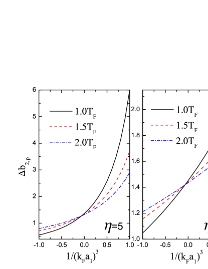
Figure 5: (Color online) The second virial coefficient $\Delta b_{2,p}^{att}$ as a function of $1/\left(k_{F}a_{1}\right)^{3}$ with finite range potential $R=0.05d$ in cigar-shaped trap $\eta=5$ and pancake-shaped trap $\eta=0.2$.

In Fig. 6 we show the second virial coefficient $\Delta b_{2,p}$ at unitarity limit $a_{1}\rightarrow\pm\infty$ as a function of dimensionless finite range of potential $R/d$. In the zero-range limit $\Delta b_{2,p}$ approaches the universal value of $3/2$ as $\tilde{\omega}=\left(3N\right)^{-1/3}\approx 0.007$ is fairly small.

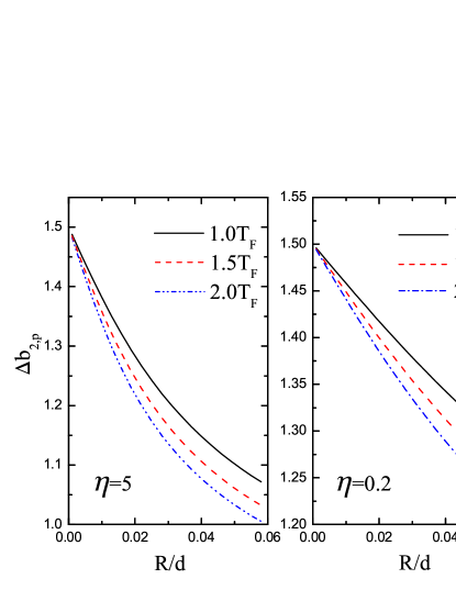
Figure 6: (Color online) The second virial coefficient $\Delta b_{2,p}$ as a function of the dimensionless finite range $R/d$ in the unitarity limit in a cigar-shaped trap ($\eta=5$) and in a pancake-shaped trap ($\eta=0.2$).

V High-$T$ thermodynamics of strongly correlated fermions

We are now in position to study the equation of state in the high-temperature regime. Using the thermodynamic relation, we have the number equation,

$$N=N^{(1)}+2\frac{\left(k_{B}T\right)^{4}}{\left(\hbar\omega\right)^{3}}\left(2\Delta b_{2}z^{2}+3\Delta b_{3}z^{3}+\cdots\right),$$ (67)

and the total energy,

$$E=-2\Omega+2\frac{\left(k_{B}T\right)^{4}}{\left(\hbar\omega\right)^{3}}\frac{T}{T_{F}}\left(\Delta b_{2}^{{}^{\prime}}z^{2}+\Delta b_{3}^{{}^{\prime}}z^{3}+\cdots\right),$$ (68)

where $\Delta b_{n}^{{}^{\prime}}\equiv d\Delta b_{n}/d\tilde{T}$ and the non-interacting number,

$$N^{(1)}=-\frac{2\left(k_{B}T\right)^{3}}{\left(\hbar\bar{\omega}\right)^{3}}\frac{1}{2}\int\limits_{0}^{\infty}t^{2}\frac{ze^{-t}}{1+ze^{-t}}dt.$$ (69)

The entropy of the system can be calculated using,

$$S=\left(E-\Omega-\mu N\right)/T,$$ (70)

where the chemical potential $\mu=k_{B}T\ln z$ (not to be confused with the reduced mass). Eqs. (53), (67), (68), together with (69), form a closed set of expressions for thermodynamics, which can be solved self-consistently.

Up to the second order virial expansion, the energy and entropy of a Fermi gas with resonant $s$-wave and $p$-wave interactions are shown in Figs. 7 and 8, respectively. Here, we consider a zero-range potential so the thermodynamics is universal. The Fermi energy is $E_{F}=k_{B}T_{F}=\left(3N\right)^{1/3}\hbar\omega$. For comparison, we show the ideal gas result using the solid lines. It is clear that the equation of state are strongly affected by interactions, even in the high temperature regime. This interaction effect is particularly apparent for $p$-wave interactions due to its large second virial coefficient.

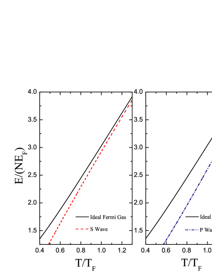
Figure 7: (Color online) Temperature dependence of the energy of a strongly correlated Fermi gas with $s$-wave and $p$-wave interactions. For comparison, we plot the ideal gas result using solid lines.

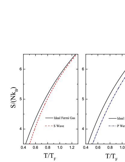
Figure 8: (Color online) Temperature dependence of the entropy of a strongly correlated Fermi gas with $s$-wave and $p$-wave interactions. The ideal gas results are shown by the solid lines.

In Figs. 9 and 10, we present the non-universal effect on thermodynamics caused by the presence of a finite-range of interaction potentials. Eqs. (64) and (66) are used in the calculations of the virial coefficient with the inclusion of the influence of the finite-range of interactions.

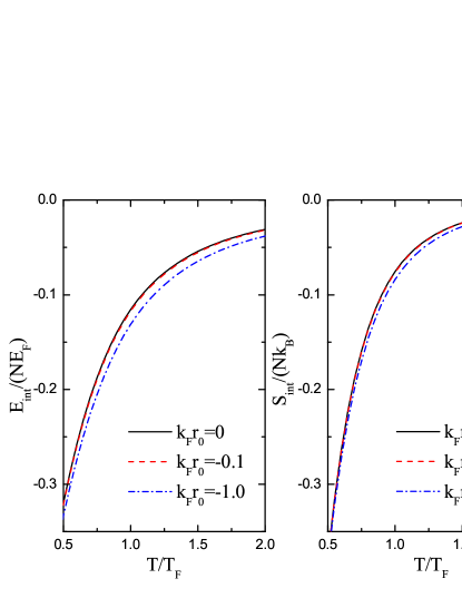
Figure 9: (Color online) The non-universal effect on the energy and entropy of a unitary $s$-wave Fermi gas. The non-universality arises from the use of a finite-range of interaction potentials.

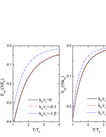
Figure 10: (Color online) The same as in Fig. 9, but for a $p$-wave resonant Fermi gas.

VI Conclusions and remarks

In conclusion, we have investigated the high-temperature thermodynamics of a strongly correlated Fermi gas with $s$-wave and $p$-wave interactions, by applying a second-order quantum virial expansion method. The second virial coefficient has been calculated, based on the numerically exact solution for two fermions in a harmonic trap. In this study, we have particularly focused on the effects arising from a finite-range interaction potential, which is crucial for $p$-wave interactions near the unitarity limit. Non-universal corrections due to the finite range corrections to the thermodynamics have been addressed.

We expect that these thermodynamic results should be useful as a complementary approach to quantum Monte Carlo simulations in understanding experimental thermodynamic measurements for a $p$-wave Fermi gas near a Feshbach resonance.

References

• (1) M. Iskin and C. A. R. Sá de Melo, Phys. Rev. Lett. 96, 040402 (2006).
• (2) S. S. Botelho and C. A. R. Sá de Melo, J. Low Temp. Phys. 140, 409 (2005).
• (3) V. Gurarie, L. Radzihovsky, and A. V. Andreev, Phys. Rev. Lett. 94, 230403 (2005).
• (4) J. Zhang, E. G. M. van Kempen, T. Bourdel, L. Khaykovich, J. Cubizolles, F. Chevy, M. Teichmann, L. Tarruell, S. J. J. M. F. Kokkelmans, and C. Salomon, Phys. Rev. A 70 030702(R) (2004).
• (5) C. A. Regal, C. Ticknor, J. L. Bohn, and D. S. Jin, Phys. Rev. Lett. 90, 053201 (2003).
• (6) K. Günter, T. Stöferle, H. Moritz, M. Köhl, and T. Esslinger, Phys. Rev. Lett. 95, 230401 (2005).
• (7) C. H. Schunck, M. W. Zwierlein, C. A. Stan, S. M. F. Raupach, W. Ketterle, A. Simoni, E. Tiesinga, C. J. Williams, and P. S. Julienne, Phys. Rev. A 71, 045601 (2005).
• (8) J. Fuchs, C. Ticknor, P. Dyke, G. Veeravalli, E. Kuhnle, W. Rowlands, P. Hannaford, and C. J. Vale, Phys. Rev. A 77, 053616 (2008).
• (9) R. A. W. Maier, C. Marzok, C. Zimmermann, and Ph. W. Courteille, Phys. Rev. A 81, 064701 (2010).
• (10) Z. Idziaszek, Phys. Rev. A 79, 062701 (2009).
• (11) T. Mizushima and K. Machida, Phys. Rev. A 81, 023624 (2010).
• (12) T. Mizushima and K. Machida, Phys. Rev. A 82, 053605 (2010).
• (13) K. Huang and C. N. Yang, Phys.Rev. 105, 767 (1957).
• (14) F. Stampfer and P. Wagner, J. Math. Anal. Appl. 342, 202 (2008).
• (15) I. Reichenbach, A. Silberfarb, R. Stock, and I. H. Deutsch, Phys. Rev. A 74, 042724 (2006).
• (16) L. Pricoupenko, Phys. Rev. Lett. 96, 050401 (2006).
• (17) K. Kanjilal and D. Blume, Phys. Rev. A 70, 042709 (2004).
• (18) R. Stock, A. Silberfarb, E. L. Bolda, and I. H. Deutsch, Phys. Rev. Lett. 94, 023202 (2005).
• (19) A. Derevianko, Phys. Rev. A 72, 044701 (2005).
• (20) E. L. Bolda, E. Tiesinga, and P . S. Julienne, Phys. Rev. A 66, 013403 (2002)
• (21) R. Roth and H. Feldmeier, Phys. Rev. A 64, 043603 (2001).
• (22) T.-L. Ho and E. J. Mueller, Phys. Rev. Lett. 92, 160404 (2004).
• (23) X.-J. Liu, H. Hu, and P. D. Drummond, Phys. Rev. Lett. 102, 160401 (2009).
• (24) H. Hu, X. J. Liu, P. D. Drummond, and H. Dong, Phys. Rev. Lett. 104, 240407 (2010).
• (25) H. Hu, X.-J. Liu, and P. D. Drummond, Phys. Rev. A 81, 033630 (2010).
• (26) T. -L. Ho and N. Zahariev, e-print arXiv:cond-mat/0408469.
• (27) T.-L. Ho, Phys. Rev. Lett. 92, 090402 (2004).
• (28) H. Hu, P. D. Drummond, and X.-J. Liu, Nature Phys. 3, 469 (2007).
• (29) H. Hu, X.-J. Liu, and P. D. Drummond, Phys. Rev. A 77, 061605 (R) (2008).
• (30) H. Hu, X.-J. Liu, and P. D. Drummond, New J. Phys. 12, 063038 (2010).
• (31) T. M. MacRobert, Spherical Harmonics (Dover Publications, New York, 1948).
• (32) N. F. Mott and H. S. W. Massey, The Theory of Atomic Collisions (Oxford U.P., London, 1965).
• (33) L. B. Madsen, Am. J. Phys. 70, 811(2002).
• (34) D. Blume and C. H. Greene, Phys. Rev. A 65, 043613 (2002).
• (35) A. Suzuki, Y. Liang, and R. K. Bhaduri, Phys. Rev. A, 80, 033601 (2009).
• (36) T. Busch, B. G. Englert, K. Rzazewski, and M. Wilkens, Found. Phys. 28, 549 (1998).
• (37) Z. Idziaszek and T. Calarco, Phys. Rev. A 74, 022712 (2006).
• (38) X.-J. Liu, H. Hu, and P. D. Drummond, Phys. Rev. A 82, 023619 (2010).