Three Regions of Excessive Flux of PeV Cosmic Rays

Abstract

Three regions of excessive flux of cosmic rays with energies of the order of PeV are found in the experimental data of the EAS MSU array at a confidence level greater than $4\sigma$. For two of them, there are similar regions in the experimental data of the EAS–1000 Prototype array. One of the interesting features of the regions is the absence of supernova remnants in their vicinities, traditionally considered as the main sources of Galactic cosmic rays, but the presence of isolated pulsars, some of which are able to accelerate heavy nuclei up to energies close to PeV. In our opinion, this favors the assumption that isolated pulsars are able to contribute to the flux of Galactic cosmic rays more than is usually assumed.

1 Introduction

The problem of the origin of cosmic rays (CRs) in the PeV energy range remains open for several decades. The model of diffusive shock acceleration at the outer front of expanding supernova remnants (SNRs) has become the most widely spread one, see, e.g., [1], though it has not been experimentally confirmed yet. Along with supernova remnants, other possible sources of PeV CRs have been considered. In particular, shortly after pulsars were discovered and identified with neutron stars, it was demonstrated that they can be effective accelerators of CRs [2]. Interest to pulsars as possible sources of CRs with energies $\gtrsim 10^{14}$ eV and up to ultrahigh energies did not vanish [3–7]. Models considered included acceleration both in pulsar wind nebulae (e.g., the Crab nebula) and by isolated pulsars. It was demonstrated in particular that the Geminga pulsar is a possible candidate for being the single source of the knee at 3 PeV [5]. There is no surprise then that one of the areas of investigations in the field are attempts to find correlation between arrival directions of CRs and coordinates of their possible astrophysical sources, including SNRs, pulsars, and some other.

In our previous works dedicated to the analysis of arrival directions of extensive air showers (EAS) registered with the EAS MSU and EAS–1000 Prototype (below, “PRO–1000”) arrays, we have already presented a number of regions of excessive flux (REFs) of PeV cosmic rays [8–11]. It was shown that not all of them could be matched with Galactic supernova remnants. However, a substantial part of REFs could be matched with isolated pulsars in whose vicinities nebulae are not observed. In this work, we consider three regions selected in the EAS MSU array data at a level of confidence greater than $4\sigma$. None of these could be matched with Galactic supernova remnants, but there are isolated pulsars inside or in close vicinities of these regions, some of which are able to accelerate heavy nuclei up to energies close to PeV. For two of these regions, there are similar regions in the PRO–1000 experimental data.

2 Experimental Data and Method of The Investigation

As in our previous studies of EAS arrival directions, the main data sets consist of 513,602 showers registered with the EAS MSU array in 1984–1990 and 1,342,340 showers of the PRO–1000 array registered in 1997–1999. A description of the arrays can be found in [12] and [13] respectively. All EAS selected for the analysis satisfy a number of quality criteria and have zenith angles $\theta<45.7^{\circ}$. Showers registered with the two arrays have different number of charged particles $N_{\rm e}$ in a typical event. For the EAS MSU array, the median value of $N_{\rm e}$ is of the order of $1.6\times 10^{5}$, while that for the PRO–1000 array equals $3.7\times 10^{4}$. According to the modern models of hadronic interactions and data on the chemical composition of cosmic rays, the given values of $N_{\rm e}$ correspond to the energies of a primary proton $E_{0}\approx 1.7\times 10^{15}$ eV and $E_{0}\approx 4.6\times 10^{14}$ eV respectively, with an error of about 10%–20%. The EAS MSU array allowed one to determine arrival directions of EAS with a better accuracy than the PRO–1000 array but the mean error is estimated to be of the order of $3^{\circ}$ in both cases.

The investigation is based on the method by Alexandreas et al., which was developed for the analysis of arrival directions of EAS registered with the CYGNUS array [14] and since then has been used multiple times for the analysis of results of other experiments on CRs. The idea of the method is as follows. To every shower in the experimental data set, arrival time of another shower is assigned in a pseudo-random way. After this, new equatorial coordinates $(\alpha,~{}\delta)$ are calculated for the “mixed” data set thus providing a “mixed” map of arrival directions. The mixed map differs from the original one but has the same distribution in declination $\delta$. In order to compare both maps, one divides them into sufficiently small “basic” cells. A measure of difference between any two regions (cells) of the two maps located within the same boundaries is defined as

$$S=(N_{\mathrm{real}}-N_{\mathrm{bg}})/\sqrt{N_{\mathrm{bg}}},$$

where $N_{\mathrm{real}}$ and $N_{\mathrm{bg}}$ are the number of EAS inside a cell in the real and “mixed” (background) maps correspondingly. The mixing of the real map is performed multiple times, and the mixed maps are averaged then in order to reduce the dependence of the result on the choice of arrival times. The method is based on an assumption that the resulting mean “background” map has most of the properties of an isotropic background, and presents the distribution of arrival directions of cosmic rays that would be registered with the array in case there is no anisotropy. Thus, deviations of the real map from the background one may be assigned to a kind of anisotropy of arrival directions of EAS registered with the array. As a rule, selection of regions of excessive flux is performed basing on the condition $S>3$.

As in [15], the basic cells have the size $0.5^{\circ}\times 0.5^{\circ}$ and the number of cycles of mixing equals 10,000. Due to this, the difference in the number of showers in basic cells of any two sequentially averaged maps by the end of the mixing cycle is of the order or (1–2)$\times 10^{-3}$ for both data sets.

The procedure of constructing cells (regions) for comparing the number of EAS falling into them is as follows. Adjacent basic strips in $\delta$ (each $0.5^{\circ}$ wide) were joined into strips of width $\Delta\delta=3^{\circ}\dots 30^{\circ}$ with the step equal to $0.5^{\circ}$. Each wide strip was then divided into adjacent cells of some fixed width $\Delta\alpha$. After this, we calculated the number of EAS inside each of these cells for both experimental ($N_{\mathrm{real}}$) and background ($N_{\mathrm{bg}}$) maps. For each pair of cells, $S$ was calculated then. A cell was considered as a possible cell of excessive flux (CEF) if $S>3$. Every wide strip was divided into cells with a shift of $0.5^{\circ}$ in the angular distance in $\alpha$ until all possible locations on the grid were covered. Contrary to [11], we did not restrict the search to cells such that $\Delta\alpha=\Delta\delta/\cos\bar{\delta}$, where $\bar{\delta}$ is the mean value of $\delta$ for the current strip, and $\Delta\alpha$ is rounded to the nearest half-integer number, but allowed $\Delta\alpha$ to deviate from that value in such a way that the area of the resulting cells deviated from the original one by 1/6. As a result, additional cells were considered. For example, besides cells of the size $\Delta\alpha\times\Delta\delta=3^{\circ}\times 3^{\circ}$, we also considered cells of the sizes $2.5^{\circ}\times 3^{\circ}$ and $3.5^{\circ}\times 3^{\circ}$. Finally, only cells with more than 100 real EAS inside were analyzed.

The method of Alexandreas et al. does not provide a direct answer to the question about the chance probability of appearance of a CEF. One is expected to calculate the corresponding probability basing on the value of $S$, which is an estimate of the standard deviation of a sample and thus acts as a significance level. It is implicitly assumed by this that the deviation of $N_{\mathrm{real}}$ from $N_{\mathrm{bg}}$ has a Gaussian distribution. Hence, the chance probability of a CEF to appear is estimated to be less than $1-0.9973$ providing it was selected at significance level $S>3$.

In order to estimate the chance probability of appearance of a CEF basing on the number of EAS inside, we introduced the following simple method based on the binomial distribution [11]. Let a shower axis getting inside the CEF be a success. The number of trials equals the number of showers $N$ in the data set under consideration, and an estimate of success (for a fixed region) equals $\tilde{p}=N_{\mathrm{bg}}/N$, where $N_{\mathrm{bg}}$ is the number of showers in the cell of the background map. The assumption is based on the fact that in the method of Alexandreas et al., $N_{\mathrm{bg}}$ is considered to be an expected number of showers in a cell. Obviously, the chance probability of finding exactly $N_{\mathrm{real}}$ EAS in a cell (or region) equals

$$P(\nu=N_{\mathrm{real}})=C(N,N_{\mathrm{real}})\tilde{p}^{N_{\mathrm{real}}}(1-\tilde{p})^{N-N_{\mathrm{real}}},$$

where $\nu$ is a random variable equal to the number of successes in the binomial model, and $C(N,N_{\mathrm{real}})$ is the corresponding binomial coefficient. It is more interesting to consider a probability that there are at most $N_{\mathrm{real}}$ showers in the cell $P_{N}=P(\nu\leq N_{\mathrm{real}})$. The analysis performed and the data presented below demonstrate that values of $P_{N}$ correlate well with the values of chance probabilities calculated on the basis of significance level $S$.

The fact that $S>3$ for a given cell does not imply it is valid for its subcells. A situation such that $S<3$ for a number of adjacent cells but $S>3$ for a cell (region) combined of them is possible. In order to improve the robustness of selection of CEFs, we have tried a number of additional quantities. One of the most efficient of them is the probability $P_{\mathrm{bc}}=P(\xi<N_{\mathrm{bc}}^{+})$, calculated from the following binomial model. Let $\xi$ be a random variable equal to the number of basic cells of the given cell with an excess of EAS over the background values, and $N_{\mathrm{bc}}^{+}$ is the corresponding experimental value. The number of trials equals the number of basic cells in the CEF. It is natural to assume the probability of success to be equal to 1/2. In the results presented below, all CEFs satisfy a condition $P_{\mathrm{bc}}>0.9545$, which corresponds to the significance level of $2\sigma$ for the Gaussian distribution. We thus reduced the chance that a CEF is selected solely due to the non-uniformity of the EAS distribution w.r.t. $\delta$.

3 Main Results and Discussion

In what follows, we consider REFs found in the EAS MSU array experimental data under the conditions

$$S>4,\quad P_{\mathrm{bc}}>0.9545,\quad N_{\mathrm{real}}>100.$$ (1)

Three regions satisfying (1) were found, see Fig. 1 and Table 1. Each of them consists of a number of partially overlapping cells, selected with the algorithm described above. The probability that any of the three REFs appears by chance is $\leq 6\times 10^{-5}$. This estimate follows from the values of $P_{N}$ shown in Table 1, as well as from the fact that $S>4$ for all the REFs: the corresponding probability equals $\approx 0.999937$ for the significance level equal to 4. Regions A and B have “partners” in the PRO–1000 data set. These are regions that satisfy conditions $S>3$, $P_{\mathrm{bc}}>0.9545$, $N_{\mathrm{real}}>100$ and partially overlap with those two regions in the EAS MSU data set.

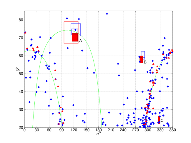
Figure 1: Location of the regions of excessive flux in equatorial coordinates. Filled with red are the three regions found in the EAS MUS data that satisfy conditions (1). The open red rectangle shows the boundaries of a region found with the condition $P_{\mathrm{bc}}>0.9545$ omitted. Blue rectangles show REFs found in the PRO–1000 data set that partially overlap with the above REFs in the EAS MSU data and satisfy conditions $S>3$, $P_{\mathrm{bc}}>0.9545$, $N_{\mathrm{real}}>100$ (“partners”). Filled red triangles show coordinates of the Galactic supernova remnants [16]. Filled blue diamonds show coordinates of the Galactic pulsars [17]. The curves at the left and right sides of the Figure show the Galactic plane, the $\cap$-like curve shows the Supergalactic plane.

Table 1: Some parameters of the REFs in the EAS MSU data set that satisfy conditions (1) (A, B, C), and their “partners” in the PRO–1000 data set (A^′, B^′). Notation: $\alpha$ and $\delta$ are the ranges of values of the corresponding coordinates; $N_{\mathrm{real}}$, $N_{\mathrm{bg}}$ are the ranges of the experimental and background flux of EAS in the cells that constitute the REF respectively, $\max S$ and $\min P_{N}$ are the maximum value of the significance level $S$ and the minimum value of $P_{N}$ for the cells that constitute the REF.

REF	$\alpha,\,^{\circ}$	$\delta,\,^{\circ}$	$N_{\mathrm{real}}$	$N_{\mathrm{bg}}$	$\max S$	$\min P_{N}$
A	115.5…130.5	68…72.5	960…1498	841.9…1350.8	4.233461	0.999962
A′	112.5…136	71…78	2034…6406	1881.4…6146.9	3.852460	0.999474
B	280…287.5	56…60	537…1029	451.5…904.3	4.478172	0.999958
B′	283…292	58…62.5	1687…3473	1552.4…3283.8	3.556190	0.999494
C	325…329.5	22…26.5	108…152	67.34…108.9	4.954917	0.999939

The median values of $N_{\rm e}$ for the regions A, B, and C are close to the value obtained for the whole data set. The region that is found around region A when omitting the condition $P_{\mathrm{bc}}>0.9545$ lies whithin the boundaries $\alpha=96^{\circ}\dots 130.5^{\circ}$ and $\delta=67^{\circ}\dots 79^{\circ}$ and contains 7386 EAS. The median value of $N_{\rm e}$ for this REF is almost equal to the value for the whole data set. The minimum values of $P_{\mathrm{bc}}$ and $P_{N}$ for the cells forming this region are equal to 0.831062 and 0.999962, respectively.

As can be seen from the Figure, there are currently no known Galactic supernova remnants in the vicinity of the regions found. Some other possible accelerators of Galactic CRs, such as X-ray binaries and OB-associations have not been found there either. There is a bright open cluster NGC 2408 at the western boundary of Region A, but the distance from it to the Solar system is unknown, and it might be difficult to obtain a reliable estimation of its contribution to the flux of Galactic PeV CRs. On the other hand, there are isolated pulsars inside or in the close vicinities of all the regions. In view of this, the question arises as to whether these pulsars could accelerate charged particles to the energies of the order of PeV?

To the best of our knowledge, there is currently no common model of acceleration of charged particles in the vicinity of isolated pulsars. To estimate the maximum energy of a particle accelerated near the light cylinder of a pulsar, we employ an expression that can be written as follows: $E_{\max}=0.34\,Z\,B\,\Omega^{2}$ eV, where $Z$ is the charge number of the particle, $B$ is the strength of the surface magnetic field, G; $\Omega$ is the angular velocity of a pulsar, rad s^-1; and the radius of the pulsar equals $10^{6}$ cm [3]. The expression was obtained under the assumption that most of the magnetic field energy in the pulsar wind zone is transformed into the kinetic energy of the particles, and the density of electron-positron pairs does not exceed $10^{-5}$ of that of ions of iron. Table 2 presents approximate values of maximum energies of protons and iron nuclei accelerated by pulsars located in the vicinities of regions A, B, and C. It can be seen that in all three cases sufficiently heavy nuclei can be accelerated up to energies close to PeV.

Table 2: Some parameters of the pulsars located near REFs A, B, and C, and estimates of the maximum energy of protons and iron nuclei. Notation: $d$ is the distance from a pulsar to the Solar system, kpc; $P$ is the barycentric period of rotation of a pulsar, s; $B$ is the strength of the surface magnetic field, G; $\dot{E}$ is the rotation energy loss, ergs/s; $\max E_{\mathrm{p}}$ and $\max E_{\mathrm{Fe}}$ are the maximum energies of a proton and an iron nucleus accelerated by a pulsar, eV.

REF	PSR Name	$d,$	$P,$	Age,	$B,$	$\dot{E},$	$\max E_{\mathrm{p}},$	$\max E_{\mathrm{Fe}},$
		kpc	s	year	G	ergs/s	eV	eV
A	J0814+7429	0.33–0.43	1.292	$1.22\cdot 10^{8}$	$4.72\cdot 10^{11}$	$3.08\cdot 10^{30}$	$4\cdot 10^{12}$	$1\cdot 10^{14}$
	J0700+6418	0.48	0.196	$4.52\cdot 10^{9}$	$1.17\cdot 10^{10}$	$3.61\cdot 10^{30}$	$4\cdot 10^{12}$	$1\cdot 10^{14}$
	J0653+8051	3.37	1.214	$5.07\cdot 10^{6}$	$2.17\cdot 10^{12}$	$8.37\cdot 10^{31}$	$2\cdot 10^{13}$	$5\cdot 10^{14}$
	J0849+8028	3.38	1.602	$5.69\cdot 10^{7}$	$8.56\cdot 10^{11}$	$4.28\cdot 10^{30}$	$4\cdot 10^{12}$	$1\cdot 10^{14}$
B	J1836+5925	0.17–0.75	0.173	$1.80\cdot 10^{6}$	$5.20\cdot 10^{11}$	$1.16\cdot 10^{34}$	$2\cdot 10^{14}$	$6\cdot 10^{15}$
	J1840+5640	1.70	1.653	$1.75\cdot 10^{7}$	$1.59\cdot 10^{12}$	$1.31\cdot 10^{31}$	$8\cdot 10^{12}$	$2\cdot 10^{14}$
C	J2155+2813	5.06	1.609	$2.78\cdot 10^{7}$	$1.23\cdot 10^{12}$	$8.68\cdot 10^{30}$	$6\cdot 10^{12}$	$2\cdot 10^{14}$
	J2156+2618	4.71	0.498	$5.56\cdot 10^{8}$	$8.51\cdot 10^{10}$	$4.53\cdot 10^{30}$	$5\cdot 10^{12}$	$1\cdot 10^{14}$
	J2151+2315	1.42	0.594	$1.33\cdot 10^{7}$	$6.56\cdot 10^{11}$	$1.34\cdot 10^{32}$	$2\cdot 10^{13}$	$6\cdot 10^{14}$
	J2139+2242	4.71	1.084	$1.21\cdot 10^{7}$	$1.26\cdot 10^{12}$	$4.41\cdot 10^{31}$	$1\cdot 10^{13}$	$4\cdot 10^{14}$

The distances to the pulsars from Table 2 exceed considerably the free path of PeV neutrons, and the amount of electromagnetic showers is insufficient for formation of REFs. In view of this, the question arises of how to keep the arrival direction of (charged) CRs propagating through the Galactic magnetic field. We are currently not ready to suggest a satisfactory model for answering this question, but we note at least two models were suggested to explain the REFs of CRs with energies of the order of 10 TeV registered with the Milagro gamma-ray observatory [18]. One of the models is based on CR acceleration in the vicinity of the Geminga pulsar [19], the properties of which are similar to those of the pulsar J1836+5925 located at the boundary of the B region [20]. The other one uses a specific magnetic field configuration able to focus a flux of charged particle [21].

To conclude, we have presented three regions of excessive flux of PeV CRs selected from the EAS MSU experimental data at a significance level $>4\sigma$ and satisfying several additional conditions. In the vicinity of every region, there are isolated Galactic pulsars that are able to accelerate sufficiently heavy nuclei to the required energies. In our opinion, this does not give enough ground to claim that the above REFs are formed due to contribution from these pulsars but can witness in favor of the assumption that (1) some isolated pulsars contribute to the flux of PeV CRs more than is usually assumed and (2) there are efficient mechanisms of focusing CR in the interstellar space.

Only free, open source software was used for the investigation. In particular, all calculations were performed with GNU Octave [22] running in Linux. This research has made use of the SIMBAD database, operated at CDS, Strasbourg, France (http://simbad.u strasbg.fr/simbad).

The research was partially supported by the Russian Foundation for Fundamental Research grant No. 08-02-00540

References

- [1] Hillas A.M., J. Phys. G 31, R95 (2005).
- [2] Gunn J.E., Ostriker J.P., Phys. Rev. Lett. 22, 728 (1969).
- [3] Blasi P., Epstein R.I., Olinto A.V., Astrophys. J. 533, L123 (2000); arXiv:astro-ph/9912240.
- [4] Giller M., Lipski M., J. Phys. G 28, 1275 (2002).
- [5] Bhadra A., Proc. 28th ICRC, Tsukuba, Japan (2003), p. 303.
- [6] Bhadra A., Astropart. Phys. 25, 226 (2006); arXiv:astro-ph/0602301.
- [7] Erlykin A.D., Wolfendale A.W., Are there pulsars in the knee?, arXiv:astro-ph/0408225.
- [8] Kulikov G.V., Zotov M.Yu., A search for outstanding sources of PeV cosmic rays: Cassiopeia A, the Crab Nebula, the Monogem Ring–But how about M33 and the Virgo cluster?, arXiv:astro-ph/0407138.
- [9] Zotov M.Yu., Kulikov, G.V., Izvestiya RAN, ser. fiz. 68, 1602 (2004).
- [10] Zotov M.Yu., Kulikov, G.V., Bull. Russ. Acad. Sci.: Physics 71, 483 (2007); arXiv:astro-ph/0610944.
- [11] Zotov M.Yu., Kulikov G.V., Izvestiya RAN, ser. fiz. 73, 612 (2009); arXiv:0902.1637.
- [12] Vernov S.N., Khristiansen G.B., Atrashkevich V.B. et al., Proc. 16th ICRC, Kyoto, 8 (1979), p. 129.
- [13] Fomin Yu.A., Igoshin A.V., Kalmykov N.N. et al., Proc. 26th ICRC, Salt Lake City, 1 (Ed. D. Kieda, M. Salamon, and B. Dingus, 1999), p. 286.
- [14] Alexandreas D.E., Berley D., Biller S. et al., Astrophys. J. 383, L53 (1991).
- [15] Zotov M.Yu., Kulikov G.V., Astronomy Letters 36, 645 (2010); arXiv:0902.3192.
- [16] Green D.A., Bull. of the Astron. Soc. of India 37, 45 (2009); arXiv:0905.3699.
- [17] Manchester R.N., Hobbs G.B., Teoh A. et al., Astrophys. J. 129, 1993 (2005). The ATNF Pulsar Database, http://www.atnf.csiro.au/research/pulsar/psrcat/
- [18] Abdo A.A., Allen B., Aune T. et al., Phys. Rev. Lett. 101, 221101 (2008); arXiv:0801.3827v3.
- [19] Salvati M., Sacco B., A&A 485, 527 (2008); arXiv:0802.2181v2.
- [20] Abdo A.A., Ackermann M., Ajello M. et al., Fermi Large Area Telescope observations of PSR J1836+5925, arXiv:1002.2977.
- [21] Drury L.O’C., Aharonian F.A., Astropart. Phys. 29, 420 (2008); arXiv:0802.4403v2.
- [22] Eaton J.W., Bateman D., Hauberg S., GNU Octave Manual Version 3 (Network Theory Ltd., United Kingdom, 2008). (http://www.octave.org/)