Network Congestion Control with Markovian Multipath Routing

Abstract

In this paper we consider an integrated model for TCP/IP protocols with multipath routing. The model combines a Network Utility Maximization for rate control based on end-to-end queueing delays, with a Markovian Traffic Equilibrium for routing based on total expected delays. We prove the existence of a unique equilibrium state which is characterized as the solution of an unconstrained strictly convex program. A distributed algorithm for solving this optimization problem is proposed, with a brief discussion of how it could be implemented by adapting the current Internet protocols.

1 Introduction

Routing and congestion control are two basic components of packet-switched communication networks. While routing is responsible for determining efficient paths along which the sources communicate to their corresponding receivers, congestion control manages the transmission rate of each source in order to keep network congestion within reasonable limits. In current practice both mechanisms belong to separate design layers that operate on different time-scales: the IP layer (Internet Protocol) determines single-path routings which are updated on a slow time-scale, while the TCP layer (Transmission Control Protocol) corresponds to end-to-end users that perform rate congestion control at a faster pace for which routing can be considered to be fixed. Scalability considerations impose that these protocols must operate in a decentralized manner.

Roughly speaking, TCP controls the rate of a source by managing a window size that bounds the maximum number of outstanding packets that have been transmitted but not yet acknowledged by the receiver. Once this window size is reached the source must wait for an acknowledgment before sending a new packet, so the rate is approximately one window of packets per round-trip time. As the network gets congested, the round-trip time increases and the transmission rate is automatically slowed down. In addition, TCP dynamically adjusts the window size of a source in response to network congestion. To this end, links generate a scalar measure of their own congestion (e.g. packet loss probability, average queue length, queueing delay) and each source is fed back a congestion signal that reflects the aggregate congestion of the links along its route. This signal is used by the source to adjust its window size so that the higher the congestion the smaller the rate. The predominant TCP protocols in use are Tahoe and Reno which use packet loss as congestion measure, and Vegas which is based on queueing delay. We refer to Low:2002 for a description and comparison of current protocols and their models.

The interaction of many sources performing a decentralized congestion control based on feedback signals that are subject to estimation errors and communication delays, gives rise to complex dynamics that are difficult to analyze. However, assuming that the dynamics stabilize on a steady state, the equilibrium can be characterized as an optimal solution of a Network Utility Maximization (NUM) problem (see Kelly:1998 ; Low:2003 ; YMR98 ). Thus, the TCP mechanism can be viewed as a decentralized algorithm that seeks to optimize an aggregate utility function subject to network constraints. The NUM approach is also useful to compare different protocols in regard to their fairness and efficiency.

A second element of packet-switched networks is routing. This function is performed by routers in a decentralized manner using routing tables that determine the next hop for each destination. The routing tables are updated periodically by an asynchronous distributed shortest path iteration that computes optimal paths according to some metric such as hop count, latency, delay, load, reliability, bandwidth, or a mixture of these. In current practice a single path that minimizes the number of hops is used for routing on each origin-destination pair. A very promising idea in traffic engineering is the use of multipath routing to increase the throughput by exploiting the available transmission capacity on a set of alternative paths. This also improves the reliability because of the ability to redirect flow into alternate paths in case of failures. While a few multipath techniques are available in today’s Internet (e.g. MPLS tunnels Villamizar:1999 or MPTCP multihoming developed by IETF Barre:2011 ), several other proposals have been tested through simulations. We defer our discussion of the relevant literature until section §5. Another relevant argument in favor of multipath routing is stability. Indeed, when route choice is based on metrics that are affected by congestion, such as queueing delay or link latencies, routing and rate control become mutually inter-dependent and equilibrium can be achieved only if both aspects are considered jointly: routing affects the rate control through the induced congestion signals, while rate control induces flows that determine in turn which routes are optimal. If routing is restricted to a single path, congestion effects may lead to route flaps. A remedy for such unstable behavior is to allow flows to split over multiple paths in order to balance their loads. An appropriate tool to capture these interactions between rate control and routing is provided by Wardrop equilibrium. On the other hand, since congestion metrics are subject to estimation errors and random effects it is natural to model routing as a stochastic equilibrium assignment.

The goal of this paper is to propose an analytical framework that provides a theoretical support for cross-layer designs for rate control under multipath routing. Our model combines rate control modeled by NUM with a routing strategy based on discrete choice distribution models that lead to a Markovian Traffic Equilibrium (MTE). The latter is a decentralized stochastic version of Wardrop’s model. The combination of the NUM and MTE models leads to a system of equations that correspond to the optimality conditions of an equivalent Markovian Network Utility Maximization problem (MNUM), a strictly convex unconstrained program of low dimension where the variables are the link congestion prices. This characterization allows us to establish the existence and uniqueness of an equilibrium, and provides a basis for designing decentralized protocols for congestion control and multipath routing.

The paper is structured as follows. Section §2 reviews the basic components of our cross-layer approach: we recall the NUM framework for modeling the steady state of TCP protocols and we discuss the concepts of Wardrop equilibrium and Markovian routing. Section §3 combines NUM and MTE, introducing the MNUM model for routing and rate control. In §3.1 we reduce MNUM to a system of equations involving only the link congestion prices, and then in §3.2 we show that these equations admit a variational characterization (d-mnum) proving the existence of a unique equilibrium state. In §4 we briefly discuss how the model might lead to a cross-layer design of a distributed TCP/IP protocol. We close the paper with comparisons to previous work and some perspectives on future research.

2 Notations and preliminaries

The communication network is modeled by a directed graph $G=(N,A)$, where the nodes $i\in N$ represent origins, destinations and intermediate routers, while the arcs $a\in A$ represent the network links. Each link is characterized by a latency function $\lambda_{a}=s_{a}(w_{a})=\lambda_{a}^{0}+\rho_{a}(w_{a})$ where $\lambda_{a}^{0}\geq 0$ represents a constant propagation delay and $\rho_{a}(w_{a})$ is the expected queueing delay expressed as a continuous and strictly increasing function $\rho_{a}:[0,c_{a})\to[0,\infty)$ of the traffic $w_{a}$ on the link, with $\rho_{a}(0)=0$ and $c_{a}\in(0,\infty]$ the maximal capacity. We also consider a finite set of sources $k\in K$ each one generating a flow rate $x^{k}\geq 0$ from an origin $s_{k}\in N$ to a destination $d_{k}\in N$.

2.1 Rate control and utility maximization under single path routing

Suppose that each source $k\in K$ routes its flow along a fixed sequence of links $(a_{1},\ldots,a_{j_{k}})$, so that the total traffic on a link $a$ is $w_{a}=\sum_{k\ni a}x^{k}$ where the summation is over all the sources $k\in K$ whose route contains that link. Consider the queueing delay $p_{a}=\rho_{a}(w_{a})$ as a measure of link congestion and assume that each source $k\in K$ adjusts its rate $x^{k}=f_{k}(q^{k})$ as a function of the aggregate queueing $q^{k}=\sum_{a\in k}p_{a}$ on its route, where $f_{k}:(0,\infty)\to(0,\infty)$ is continuous and strictly decreasing with $f_{k}(q^{k})\to 0$ as $q^{k}\to\infty$. These equilibrium equations may be written as

$$f_{k}^{-1}(x^{k})=q^{k}=\sum_{a\in k}p_{a}=\sum_{a\in k}\rho_{a}(w_{a})=\sum_{a\in k}\rho_{a}(\mbox{$\sum_{s\ni a}x^{s}$})$$

which correspond to the optimality conditions for the strictly convex program

$$\min_{x\in{\mathbb{R}}^{K}}\sum_{a\in A}R_{a}(\mbox{$\sum_{s\ni a}x^{s}$})-\sum_{k\in K}\int_{0}^{x^{k}}\!\!\!\!f_{k}^{-1}(z)dz$$ (num)

where $R_{a}(\cdot)$ denotes a primitive of $\rho_{a}(\cdot)$. Alternatively, the equations may be stated in terms of the queueing delays as

$$\rho_{a}^{-1}(p_{a})=w_{a}=\sum_{k\ni a}x^{k}=\sum_{k\ni a}f_{k}(q^{k})=\sum_{k\ni a}f_{k}(\mbox{$\sum_{b\in k}p_{b}$})$$

which are the optimality conditions for the strictly convex dual program

$$\min\limits_{p\in{\mathbb{R}}^{A}}\sum\limits_{a\in A}\int_{0}^{p_{a}}\!\!\!\rho_{a}^{-1}(y)\,dy-\sum\limits_{k\in K}F_{k}(\mbox{$\sum_{b\in k}p_{b}$})$$ (d-num)

where $F_{k}(\cdot)$ is a primitive of $f_{k}(\cdot)$.

Example. Consider the model for TCP Vegas proposed in Low:2003 ; LPW:2002 . For each source $k$ and time $t$, let $W^{k}_{t}$ denote the size of the congestion window and $T^{k}_{t}=D^{k}+q^{k}_{t}$ the RTT expressed as the sum of the total propagation delay $D^{k}$ and the queueing delay $q^{k}_{t}$. A Vegas source estimates $D^{k}$ as the minimum observed RTT, and tries to keep the difference between the expected rate $\hat{x}^{k}_{t}=W^{k}_{t}/D^{k}$ and the actual rate $x^{k}_{t}=W^{k}_{t}/T^{k}_{t}$ close to a given value $\alpha^{k}>0$. To this end, the congestion window is increased if $\hat{x}^{k}_{t}-x^{k}_{t}<\alpha^{k}$, and decreased when $\hat{x}^{k}_{t}-x^{k}_{t}>\alpha^{k}$. At equilibrium we must have $\hat{x}^{k}-x^{k}=\alpha^{k}$ which yields the equilibrium rate functions

$$x^{k}=\frac{\alpha^{k}D^{k}}{q^{k}}\triangleq f_{k}(q^{k}).$$

A simple model for queueing delay can be obtained by considering each link as an M/M/1 queue with service rate $c_{a}>0$ and an infinite buffer, which gives the expected queueing delay

$$p_{a}=\frac{w_{a}}{c_{a}(c_{a}-w_{a})}\triangleq\rho_{a}(w_{a}).$$

The (num) formalism can handle other congestion measures besides queueing delay and has been used to model the steady state of different TCP protocols, each one characterized by specific maps $f_{k}$ and $\rho_{a}$ (see Dumas:2001 ; Gibbens:1999 ; Kelly:1998 ; Kunniyur:2003 ; Low:2002 ; Padhye:2000 ).

2.2 Routing and traffic equilibrium

We review next some equilibrium models for traffic routing in congested networks. In this setting the source flow rates $x^{k}$ are fixed but may be routed along a set of alternative paths $R^{k}$ connecting the origin $s_{k}$ to the destination $d_{k}$. The basic modeling principle introduced by Wardrop in Wardrop:1952 is that at equilibrium only paths that are optimal should be used to route flow.

In contrast with rate control which uses queueing delay $p_{a}=\rho_{a}(w_{a})$, route optimality will be measured using the total delays $\lambda_{a}=\lambda_{a}^{0}+\rho_{a}(w_{a})$ so that packets are routed along paths with smaller round trip times and not only small queuing delays. The rationale is that the earlier each packet is delivered, the larger the rate. The protocol should automatically select the most efficient routes, depending on the congestion prevailing on each link. A further advantage of choosing the currently shortest path using total delay is to ensure that packets arrive in order to their destination, reducing the conflicts with the duplicate ack mechanism for detecting packet losses in TCP.

Example. To illustrate the point, consider two parallel links with identical queuing capacity but one of them with much longer propagation delay. A routing based on queuing delay alone would yield a 50% traffic split, with ack delays dominated by the slow link which unnecessarily limits the transmission rate (the fast link being under-utilized). Instead, a routing based on total delay will use the fast link more intensively until increased queuing makes the slow link competitive, achieving a higher throughput. Naturally, the fast link will have a larger queue as compared to the slow link, but not larger than in single-path routing as long as TCP is still controlling the amount of traffic using the Vegas mechanism. Eventually, a very slow link will not be used at all, which is again consistent with supporting higher rates.

2.2.1 Wardrop equilibrium

Suppose that the flow $x^{k}$ is split into non-negative path-flows $h_{r}\geq 0$ so that $x^{k}=\sum_{r\in R^{k}}h_{r}$, and let $w_{a}=\sum_{r\ni a}h_{r}$ be the induced total link-flows. Let $H$ denote the set of such feasible flows $(h,w)$. An equilibrium Wardrop:1952 is characterized by the fact that only optimal paths are used, namely, for each destination $k\in K$ and each route $r\in R^{k}$ one has

$$h_{r}>0\Rightarrow c_{r}=\tau_{k}$$ (1)

where $c_{r}=\sum_{a\in r}\lambda_{a}=\sum_{a\in r}s_{a}(w_{a})$ denotes the total delay of the route and $\tau_{k}=\min_{r\in R^{k}}c_{r}$ is the minimum cost faced by source $k$.

These equilibria were characterized in Beckmann:1956 as the optimal solutions of the convex program

$$\min\limits_{(h,w)\in H}\sum\limits_{a\in A}\int_{0}^{w_{a}}\!\!\!s_{a}(z)\,dz.$$ (p-w)

Since the feasible set $H$ is compact this problem has optimal solutions, while strict convexity implies that the optimal $w$ is unique. Alternatively, the equilibrium delays $\lambda_{a}=s_{a}(w_{a})$ are the unique optimal solution of the strictly convex unconstrained dual problem

$$\min\limits_{\lambda\in{\mathbb{R}}^{A}}\sum\limits_{a\in A}\int_{\lambda_{a}^{0}}^{\lambda_{a}}\!\!\!s_{a}^{-1}(z)\,dz-\sum_{k\in K}x^{k}\tau_{k}(\lambda)$$ (d-w)

where $\lambda_{a}^{0}=s_{a}(0)$ and $\tau_{k}(\lambda)\triangleq\min_{r\in R^{k}}\sum_{a\in r}\lambda_{a}$ is the minimum total delay for source $k\in K$.

Remark. The well known Braess’ Paradox indicates that there are situations in which forbidding flow on some links might lead to a modified equilibrium where all sources benefit from smaller travel times. This raises the relevant question of which links should be forbidden to optimize network performance. Unfortunately, as shown in Roughgarden:2006 this problem turns out to be hard to solve even approximately and even for a single source. Namely, unless P=NP, there is no polynomial approximation algorithm with approximation ratio less than $n/2$ where $n$ the number of nodes, while the optimal ratio $n/2$ is trivially attained by forbidding no link. As a consequence, harmful links cannot be detected efficiently. To compensate, it is worth mentioning that for sufficiently high levels of demand and congestion, Braess’ Paradox does not occur (see Nagourney:2010 ).

2.2.2 Markovian routing and equilibrium

When link delays are subject to stochastic variability, the route delays $\tilde{c}_{r}$ become random variables and the equilibrium conditions (1) are replaced by a stochastic assignment of the form $h_{r}=x^{k}\,{\mathbb{P}}(\mbox{$\tilde{c}_{r}$ is optimal})$. For instance, if the costs $\tilde{c}_{r}$ are i.i.d. Gumbel variables with expected value $c_{r}={\mathbb{E}}(\tilde{c}_{r})$, we get the Logit distribution rule common in the transportation literature

$$h_{r}=x^{k}{\exp(-\beta c_{r})\over\sum_{p\in R^{k}}\exp(-\beta c_{p})}\quad\quad(\forall\,r\in R^{k})$$

which assigns flow to all the paths, favoring those with smaller expected cost $c_{r}$. The parameter $\beta$ controls how concentrated is the repartition: for $\beta\sim 0$ every path receives an approximately equal share of the flow, while for $\beta$ large the flow concentrates on paths with minimal cost. Unfortunately, given the exponential number of end-to-end paths, such route-based distribution rules controlled directly by sources do not seem amenable to design decentralized scalable routing protocols. This becomes critical if the protocol is expected to be responsive when facing route delays that vary with traffic congestion.

An alternative is to conceive routing as a stochastic dynamic programming process. Suppose that each packet experiences a random delay $\tilde{\lambda}_{a}$ when traversing link $a$, and let $\tilde{\tau}_{i}^{k}$ be a random variable that represents the total delay from node $i$ to destination $d_{k}$. Denote $\lambda_{a}={\mathbb{E}}(\tilde{\lambda}_{a})$ and $\tau_{i}^{k}={\mathbb{E}}(\tilde{\tau}_{i}^{k})$ their expected values.

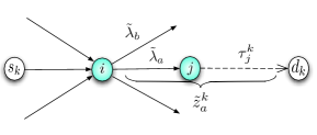
Figure 1: Variables for dynamic programming equations

If a packet at node $i$ is routed through the link $a\in A_{i}^{+}$ we have $\tilde{\tau}_{i}^{k}=\tilde{\lambda}_{a}+\tilde{\tau}_{j_{a}}^{k}$, so that a shortest path routing should choose the link with smallest $\tilde{\lambda}_{a}+\tilde{\tau}_{j_{a}}^{k}$. Unfortunately, while the link delays $\tilde{\lambda}_{a}$ for $a\in A_{i}^{+}$ might be observed at node $i$, this is not the case for the $\tilde{\tau}_{j_{a}}^{k}$’s which depend on future delays that will be experienced when traversing the downstream links. Suppose instead that only the expected values $\tau_{j_{a}}^{k}$ are known and available at node $i$ and that each packet from source $k\in K$ observes the $\tilde{\lambda}_{a}$’s and is routed through the link $a\in A_{i}^{+}$ that minimizes $\tilde{z}_{a}^{k}=\tilde{\lambda}_{a}+\tau_{j_{a}}^{k}$ to the next node $j_{a}$ where the process repeats. Thus, denoting $E_{a}^{k}\triangleq\{\tilde{z}_{a}^{k}\leq\tilde{z}_{b}^{k}\,\,\,\forall b\in A_{i}^{+}\}$, the packets from source $k\in K$ move across the network according to a Markov chain with transition probabilities

$$P_{ij}^{k}=\left\{\begin{array}[]{cl}{\mathbb{P}}(E_{a}^{k})&\mbox{if }ij=a\\[4.30554pt] 0&\mbox{otherwise}\end{array}\right.$$ (2)

for $i\neq d_{k}$, while the destination $d_{k}$ is an absorbing state. The expected flows correspond to the invariant measures of these Markov chains, leading to a flow distribution rule in which the throughput flow $y_{i}^{k}$ from source $k$ that enters node $i$, splits among the links $a\in A_{i}^{+}$ according to (see Figure 2)

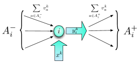
Figure 2: Flow conservation diagram (here $i=s_{k}$)

$$v_{a}^{k}=y_{i}^{k}\;{\mathbb{P}}(E_{a}^{k}).$$ (3)

The throughputs $y^{k}=(y_{i}^{k})_{i\neq d_{k}}$ can be computed from the stationary equations $y^{k}=\sum_{j=0}^{\infty}[(\hat{P}^{k})^{\prime}]^{j}\delta^{k}x^{k}$, where $\hat{P}^{k}=(P_{ij}^{k})_{i,j\neq d_{k}}$ is the reduced transition matrix on the non-absorbing states, and $\delta_{i}^{k}=1$ for $i=s_{k}$ and $\delta_{i}^{k}=0$ otherwise. This may also be written as $y^{k}=x^{k}\delta^{k}+(\hat{P}^{k})^{\prime}y^{k}$ which corresponds to the standard flow conservation equations

$${y_{i}^{k}=x^{k}\delta_{i}^{k}+\mbox{$\sum_{a\in A_{i}^{-}}$}v_{a}^{k}}.$$ (4)

These equations can be restated compactly using expected utility theory. Namely, let us write $\tilde{z}_{a}^{k}=z_{a}^{k}+\epsilon_{a}^{k}$ as the sum of its expected value $z_{a}^{k}=\lambda_{a}+\tau_{j_{a}}^{k}$ plus a noise $\epsilon_{a}^{k}$ with ${\mathbb{E}}(\epsilon_{a}^{k})=0$, and assume that the distribution of $\epsilon_{a}^{k}$ does not change with $z_{a}^{k}$ (for a discussion of this assumption see §6). Also, for simplicity $\epsilon_{a}^{k}$ is supposed to have continuous distribution so that the expected utility functions introduced next will be differentiable (distributions with point masses can be treated as in Cominetti:2008 ). Under these assumptions, the transition probabilities in (2) can be expressed as ${\mathbb{P}}(E_{a}^{k})=\frac{\partial\varphi_{i}^{k}}{\partial z_{a}^{k}}(z^{k})$ where $\varphi_{i}^{k}$ denote the expected utility functions

$$\varphi_{i}^{k}(z^{k})=\left\{\begin{array}[]{cl}{\mathbb{E}}(\min\limits_{a\in A_{i}^{+}}\{z_{a}^{k}+\epsilon_{a}^{k}\})&\mbox{if $i\neq d_{k}$}\\[8.61108pt] 0&\mbox{if $i=d_{k}$}\end{array}\right.$$ (5)

which allow us to rewrite the flow equations (3)-(4) as

$${\left\{\begin{array}[]{ll}v_{a}^{k}=y_{i}^{k}\,\frac{\partial\varphi_{i}^{k}}{\partial z_{a}^{k}}(z^{k})&\,\,\forall a\in A_{i}^{+}\\[4.30554pt] y_{i}^{k}=x^{k}\delta_{i}^{k}+\sum_{a\in A_{i}^{-}}v_{a}^{k}&\,\,\forall i\neq d_{k}.\end{array}\right.}$$ (6)

On the other hand, assuming that the cost-to-go variables $\{\tilde{\tau}_{j_{a}}^{k}:a\in A_{i}^{+}\}$ are independent from the local queueing times $\{\tilde{\lambda}_{a}:a\in A_{i}^{+}\}$, we may compute the expected value of $\tilde{\tau}_{i}^{k}$ by conditioning on the events $E_{a}^{k}$ as

$$\tau_{i}^{k}={\mathbb{E}}(\tilde{\tau}_{i}^{k}) = \sum_{a\in A_{i}^{+}}{\mathbb{E}}(\tilde{\lambda}_{a}+\tilde{\tau}_{j_{a}}^{k}|E_{a}^{k}){\mathbb{P}}(E_{a}^{k})$$

$$= \sum_{a\in A_{i}^{+}}{\mathbb{E}}(\tilde{\lambda}_{a}+\tau_{j_{a}}^{k}|E_{a}^{k}){\mathbb{P}}(E_{a}^{k})$$

$$= {\mathbb{E}}(\min\limits_{a\in A_{i}^{+}}\{\tilde{\lambda}_{a}+\tau_{j_{a}}^{k}\})$$

so that

$$\left\{\begin{array}[]{ll}\tau_{i}^{k}={\varphi}_{i}^{k}(z^{k})&\forall i\in N\\[4.30554pt] z_{a}^{k}=\lambda_{a}+\tau_{j_{a}}^{k}&\forall a\in A.\end{array}\right.$$ (7)

Under mild conditions it was proved in Cominetti:2008 that, given the $\lambda_{a}$’s, system (6)-(7) has a unique solution $(v,y,\tau,z)$. It was also shown that these equations, together with the equilibrium conditions $\lambda_{a}=s_{a}(w_{a})$ where $w_{a}=\sum_{k\in K}v_{a}^{k}$ represents the total expected link load, have a unique solution $(\lambda,w,v,y,\tau,z)$ called a Markovian Traffic Equilibrium (MTE). This equilibrium is characterized by a pair of dual optimization problems analog to (p-w) and (d-w). As a matter of fact, the dual problem has exactly the same form

$$\min\limits_{\lambda\in{\mathbb{R}}^{A}}\sum\limits_{a\in A}\int_{\lambda_{a}^{0}}^{\lambda_{a}}\!\!\!s_{a}^{-1}(z)\,dz-\sum_{k\in K}x^{k}\tau_{k}(\lambda)$$ (d-mte)

where $\tau_{k}(\lambda)\triangleq\tau_{s_{k}}^{k}(\lambda)$ with $\tau_{i}^{k}(\lambda)$ the solution of (7).

The expected utility maps $\varphi_{i}^{k}(\cdot)$ convey all the information required to describe a Markovian routing and may be considered as the primary modeling objects. These maps are determined by the random variables $\epsilon_{a}^{k}$ which are ultimately tied to the arc random costs $\tilde{\lambda}_{a}$. The class $\mathcal{E}$ of maps that can be expressed in the form (5) admits an analytic characterization (see Cominetti:2008 ): they are the $\mathcal{C}^{1}$ maps ${\varphi}:{\mathbb{R}}^{n}\to{\mathbb{R}}$ that are concave, componentwise non-decreasing, and which satisfy in addition

1. ${\varphi}(x_{1}+c,\ldots,x_{n}+c)={\varphi}(x_{1},\ldots,x_{n})+c$

2. ${\varphi}(x)\to x_{i}$ when $x_{j}\to\infty$ for all $j\neq i$

3. for $x_{i}$ fixed, $\frac{\partial{\varphi}}{\partial x_{i}}(x_{1},\ldots,x_{n})$ is a continuous distribution function on the remaining variables.

Note also that ${\varphi}(x)\leq\min\{x_{1},\ldots,x_{n}\}$. In what follows we assume that the model is specified directly in terms of a family of maps $\varphi_{i}^{k}\in\mathcal{E}\!$ with $\varphi_{d_{k}}^{k}\equiv 0$. However, we note that these maps are not used explicitly by our distributed protocol in Section §4.

Remark. Since packet movements are governed by a Markov chain, cycling may occur and additional conditions are required to ensure that packets reach the destination with probability one. A simple case is when source $k$ considers only the arcs in $A_{i}^{+}$ that lead closer to destination $d_{k}$ (e.g. $\tau_{j_{a}}^{k}<\tau_{i_{a}}^{k}$), so that the corresponding Markov chain is supported over an acyclic graph $(N,A^{k})$. To deal with this case it suffices to redefine

$$\varphi_{i}^{k}(z^{k})\triangleq{\mathbb{E}}(\min_{a\in A_{i}^{k+}}\{z_{a}^{k}+\epsilon_{a}^{k}\})$$

so that $P_{ij}^{k}=\mbox{$\frac{\partial\varphi_{i}^{k}}{\partial z_{a}^{k}}(z^{k})$}=0$ for all $a\!=\!ij\!\not\in\!A_{i}^{k+}\!\!$.

3 Rate control with Markovian routing

We proceed to develop a cross-layer model that combines a NUM approach for rate control based on queueing delays, with a Markovian multipath routing based on total delays. Each source $k\in K$ is characterized by an origin $s_{k}$, a destination $d_{k}$, and a continuous decreasing rate function $f_{k}:(0,\infty)\to(0,\infty)$ with $f_{k}(q^{k})\to 0$ as $q^{k}\to\infty$, while every link $a\in A$ has a continuous increasing latency function $s_{a}:[0,c_{a})\to[\lambda_{a}^{0},\infty)$ with $\lambda_{a}^{0}=s_{a}(0)\geq 0$. Packets are routed according to a Markovian strategy characterized by a family of maps ${\varphi}_{i}^{k}\in\mathcal{E}$ with ${\varphi}_{d_{k}}^{k}\equiv 0$. Sources adjust their rates as a function $x^{k}=f_{k}(q^{k})$ of the total queueing delay $q^{k}=\tau_{k}(\lambda)-\tau_{k}^{0}$, where $\tau_{k}(\lambda)$ is the end-to-end expected delay defined in the previous section and $\tau_{k}^{0}$ is the minimal travel time considering propagation delays only.

Informally, the source rates $x^{k}$ induce flows $v_{a}^{k}$ and total link loads $w_{a}$. These loads determine link expected delays $\lambda_{a}=s_{a}(w_{a})$ that yield end-to-end delays $\tau_{k}(\lambda)$ for each source and corresponding queueing delays $q^{k}$. At equilibrium, these queueing delays must induce the original rates $x^{k}=f_{k}(q^{k})$.

Definition 1

A pair $(w,x)$ with $w=(w_{a})_{a\in A}$ and $x=(x^{k})_{k\in K}$ is called a Markovian Network Utility Maximization (MNUM) equilibrium if and only if $w_{a}=\sum_{k\in K}v_{a}^{k}$  where $(v^{k},y^{k})$ solve the flow conservation constraints (6) with $(\tau^{k},z^{k})$ satisfying (7), together with the link delay relations $\lambda_{a}=s_{a}(w_{a})$ and the rate equilibrium conditions $x^{k}=f_{k}(q^{k})$ where $q^{k}=\tau_{k}(\lambda)-\tau_{k}^{0}$.

3.1 Reduced formulation of MNUM

In order to establish the existence and uniqueness of equilibria we begin by reducing MNUM to an equivalent set of equations that involves only the variables $\lambda$. To this end we need to extend the results in Cominetti:2008 for which we consider a fixed non-negative link delay vector $(\lambda_{a})_{a\in A}$. We first show that (7) uniquely defines $z^{k}$ and $\tau^{k}$ as implicit functions of $\lambda$. This system can be equivalently stated solely in terms of the variables $\tau^{k}$ as

$${\tau_{i}^{k}={\varphi}_{i}^{k}\left((\lambda_{a}+\tau_{j_{a}}^{k})_{a\in A}\right)}$$ (8)

so it suffices to prove that the latter uniquely defines $\tau^{k}$ as a function of $\lambda$.

Proposition 1

Let $k\in K$ and denote ${\bar{\tau}_{i}^{k}}$ the cost of a shortest path from $i$ to destination $d_{k}$ with link costs $\lambda_{a}$. Suppose also that $\hat{\tau}^{k}\in{\mathbb{R}}^{N}$ is such that

$$\hat{\tau}^{k}_{i}\leq{\varphi}_{i}^{k}((\lambda_{a}+\hat{\tau}^{k}_{j_{a}})_{a\in A})\quad\quad(\forall\,i\in N).$$ (9)

Then $\hat{\tau}^{k}\!\leq\!\bar{\tau}^{k}$ and moreover, starting from $\tau^{k,0}\!=\!\bar{\tau}^{k}$, the iterates computed by

$${\tau_{i}^{k,n+1}=\varphi_{i}^{k}((\lambda_{a}+\tau_{j_{a}}^{k,n})_{a\in A})}\quad\quad n=0,1,2\ldots$$ (10)

are non-increasing and converge to a solution $\tau^{k}$ of (8) with $\tau_{i}^{k}\in[\hat{\tau}_{i}^{k},\bar{\tau}_{i}^{k}]$.

Proof

In order to prove that $\hat{\tau}^{k}\leq\bar{\tau}^{k}$ let ${\cal I}=\{i:\hat{\tau}_{i}^{k}\leq\bar{\tau}_{i}^{k}\}$ and suppose by contradiction ${\cal I}\neq N$. Since $\hat{\tau}_{d_{k}}^{k}\leq 0=\bar{\tau}_{d_{k}}^{k}$ we have $d_{k}\in{\cal I}$. Consider a shortest path from a node $i_{0}\not\in{\cal I}$ to $d_{k}$, and let $i\not\in{\cal I}$ be the last node before entering ${\cal I}$ and $j\in{\cal I}$ the next node. Since ${\varphi}_{i}^{k}(z^{k})\leq\min_{a\in A_{i}^{+}}z_{a}^{k}$ we get

$$\hat{\tau}_{i}^{k} \leq \varphi_{i}^{k}((\lambda_{a}+\hat{\tau}_{j_{a}}^{k})_{a\in A})$$

$$\leq \lambda_{ij}+\hat{\tau}_{j}^{k}\leq\lambda_{ij}+\bar{\tau}_{j}^{k}=\bar{\tau}_{i}^{k}<\hat{\tau}_{i}^{k}.$$

This contradiction proves that $\hat{\tau}^{k}\leq\bar{\tau}^{k}$.

Let us prove next the convergence of the iteration (10). We note that

$$\tau_{i}^{k,1} = {\varphi}^{k}_{i}((\lambda_{a}+\tau_{j_{a}}^{k,0})_{a\in A})$$

$$\leq \min_{a\in A_{i}^{+}}\{\lambda_{a}+\bar{\tau}_{j_{a}}\}=\bar{\tau}_{i}=\tau_{i}^{k,0}$$

from which it follows inductively that the sequence (10) is non-increasing: if $\tau^{k,n}\leq\tau^{k,n-1}$ then

$$\tau_{i}^{k,n+1} = {\varphi}^{k}_{i}((\lambda_{a}+\tau_{j_{a}}^{k,n})_{a\in A})$$

$$\leq {\varphi}^{k}_{i}((\lambda_{a}+\tau_{j_{a}}^{k,n-1})_{a\in A})=\tau_{i}^{k,n}.$$

It remains to show that the sequence $\tau^{k,n}$ is bounded below by $\hat{\tau}^{k}$. We prove this by induction: the base case $\tau^{k,0}=\bar{\tau}^{k}\geq\hat{\tau}^{k}$ was just proved above, while for the induction step it suffices to note that $\tau^{k,n}\geq\hat{\tau}^{k}$ implies

$$\tau_{i}^{k,n+1} = {\varphi}^{k}_{i}((\lambda_{a}+\tau_{j_{a}}^{k,n})_{a\in A})$$

$$\geq {\varphi}^{k}_{i}((\lambda_{a}+\hat{\tau}_{j_{a}}^{k})_{a\in A})\geq\hat{\tau}^{k}_{i}.$$

By continuity it follows that the limit of $\tau^{k,n}$ satisfies (8) and $\tau_{i}^{k}\in[\hat{\tau}_{i}^{k},\bar{\tau}_{i}^{k}]$. $\Box$

Remark. The previous result gives a procedure to solve (8): compute the shortest path delays $\bar{\tau}^{k}$ and then iterate (10). Alternatively one may start from $\tau^{k,0}=\hat{\tau}^{k}$ in which case the iterates increase and are bounded from above by $\bar{\tau}^{k}$, hence these iterates also converge to a solution of (8).

Definition 1

We denote $\mathcal{P}$ the set of all $\lambda\in{\mathbb{R}}^{A}$ such that for each destination $k\in K$ there exists $\hat{\tau}^{k}\in{\mathbb{R}}^{N}$ satisfying

$$\hat{\tau}_{i}^{k}<{\varphi}_{i}^{k}((\lambda_{a}+\hat{\tau}_{j_{a}}^{k})_{a\in A})\mbox{ for all }i\neq d_{k}.$$ (11)

Note that $\mathcal{P}$ is an open convex domain, and for each $\lambda\in{\cal P}$ we have $\lambda^{\prime}\in{\cal P}$ for all $\lambda^{\prime}\geq\lambda$. In the sequel we extend the results in Cominetti:2008 which were based on a much more stringent condition assuming that (11) holds with $\hat{\tau}^{k}=0$. The proofs differ substantially so we present them below.

Lemma 1

Let $\lambda\in{\cal P}$ and suppose that $(\tau^{k},z^{k})$ solves (7). Let $\hat{Q}^{k}(z^{k})$ be the matrix with entries $\hat{Q}_{ia}^{k}(z^{k})={\partial{\varphi}_{i}^{k}\over\partial z_{a}^{k}}(z^{k})$ for $i\neq d_{k}$ and $a\in A$. Then

1. For each $i\!\neq\!d_{k}$ there exists $j\!\in\!N$ such that $P_{ij}^{k}\!>\!0$ and $\hat{\tau}_{j}^{k}-\tau_{j}^{k}>\hat{\tau}_{i}^{k}-\tau_{i}^{k}$.

2. The matrix $[I-\hat{P}^{k}(z^{k})]$ is invertible.

3. Equation (6) has a unique solution given by $v^{k}=\hat{Q}^{k}(z^{k})^{{}^{\prime}}y^{k}\!\geq\!0$ with $y^{k}\!=\![I\!-\!\hat{P}^{k}(z^{k})^{{}^{\prime}}]^{-1}\delta^{k}x^{k}\!\geq\!0$.

Proof

(a) Since the ${\varphi}_{i}^{k}$’s are concave and differentiable we have

$$\begin{array}[]{rcl}\hat{\tau}_{i}^{k}&<&{\varphi}_{i}^{k}((\lambda_{a}+\hat{\tau}_{j_{a}}^{k})_{a\in A})\\ &\leq&{\varphi}_{i}^{k}(z^{k})+\sum\limits_{a\in A}\frac{\partial{\varphi}_{i}^{k}}{\partial z_{a}^{k}}(z^{k})(\hat{\tau}_{j_{a}}^{k}-\tau_{j_{a}}^{k})\\ &=&\tau_{i}^{k}+\sum\limits_{ij\in A_{i}^{+}}P_{ij}^{k}(\hat{\tau}_{j}^{k}-\tau_{j}^{k})\end{array}$$

from which (a) follows directly.

(b) Given $i\neq d_{k}$ and using (a) inductively we can find a finite sequence of nodes $i_{0},\ldots,i_{m}$ with $i_{0}=i,i_{m}=d_{k}$ and $P_{i_{k}i_{k+1}}>0$. Thus, starting from $i$, the chain has a positive probability of reaching the absorbing state $d_{k}$ in a finite number of steps. This implies that $\hat{P}^{k}(z^{k})^{m}$ is strictly submarkovian for $m$ large enough, and therefore $[I-\hat{P}^{k}(z^{k})]$ is invertible.

(c) The first equation of (6) can be rewritten as $v^{k}=\hat{Q}^{k}(z^{k})^{{}^{\prime}}y^{k}$, which substituted into the second equation yields $y^{k}=\delta^{k}x^{k}+\hat{P}^{k}(z^{k})^{{}^{\prime}}y^{k}$, so that (b) implies $y^{k}=[I-\hat{P^{k}}(z^{k})^{{}^{\prime}}]^{-1}\delta^{k}x^{k}$. The non-negativity of these quantities follows from the fact that $x^{k}\geq 0$ while the matrices $\hat{Q}^{k}(z^{k})$ and $\hat{P^{k}}(z^{k})$ have non-negative entries with $[I-\hat{P^{k}}(z^{k})^{{}^{\prime}}]^{-1}=\sum_{m=0}^{\infty}[\hat{P^{k}}(z^{k})^{{}^{\prime}}]^{m}$. $\Box$

The next result is the key to reduce the MNUM equations to a system in the variables $\lambda$.

Proposition 2

If $\lambda\in{\cal P}$ then, for each source $k\in K$, the system (7) has a unique solution $z^{k}=z^{k}(\lambda)>0$ and $\tau^{k}=\tau^{k}(\lambda)>0$. Moreover, the functions $\lambda\to\tau_{i}^{k}(\lambda)$ and $\lambda\to z_{a}^{k}(\lambda)$ are concave, smooth and component-wise non-decreasing.

Proof

It suffices to show that (8) defines implicit maps $\lambda\mapsto\tau_{i}^{k}(\lambda)$ over the domain ${\cal P}$ which are well defined, concave, smooth, and monotone. We already proved the existence of a solution with $\tau_{i}^{k}\geq\hat{\tau}_{i}^{k}$. Let us prove its uniqueness.

Uniqueness: Let $k\in K$ and consider two solutions $(\tau^{1},z^{1})$ and $(\tau^{2},z^{2})$ for (7). Let $\alpha=\max_{i\in N}(\tau_{i}^{2}-\tau_{i}^{1})$ and denote $N^{\ast}$ the set of nodes where the maximum is attained. For every $i\in N^{\ast}$, the concavity of ${\varphi}_{i}^{k}(\cdot)$ gives

$$\tau_{i}^{2}={\varphi}_{i}^{k}(z^{2}) \leq {\varphi}_{i}^{k}(z^{1})+\mbox{$\sum_{a\in A_{i}^{+}}\frac{\partial{\varphi}_{i}^{k}}{\partial z_{a}^{k}}$}(z^{1})(z_{a}^{2}-z_{a}^{1})$$

$$= \tau_{i}^{1}+\mbox{$\sum_{a\in A_{i}^{+}}\frac{\partial{\varphi}_{i}^{k}}{\partial z_{a}^{k}}$}(z^{1})(\tau_{j_{a}}^{2}-\tau_{j_{a}}^{1})$$

and, since $(\tau_{j_{a}}^{2}-\tau_{j_{a}}^{1})\leq\alpha$ while the partial derivatives add up to 1, we get

$$\alpha=\tau_{i}^{2}-\tau_{i}^{1}\leq\mbox{$\sum_{a\in A_{i}^{+}}\frac{\partial{\varphi}_{i}^{k}}{\partial z_{a}^{k}}(z^{1})$}(\tau_{j_{a}}^{2}-\tau_{j_{a}}^{1})\leq\alpha.$$

It follows that for every $a\in A_{i}^{+}$ such that $\frac{\partial{\varphi}_{i}^{k}}{\partial z_{a}^{k}}(z^{1})>0$ we necessarily have $j_{a}\in N^{\ast}$. Combining this fact with Lemma 1(a), we can find a finite sequence of nodes in $N^{\ast}$ starting at $i$ and ending at $d_{k}$. Hence $d_{k}\in N^{\ast}$ so that $\alpha=\tau_{d_{k}}^{2}-\tau_{d_{k}}^{1}=0$, which implies $\tau^{2}\leq\tau^{1}$. Exchanging the roles of $\tau^{1}$ and $\tau^{2}$ we get the converse inequality so that $\tau^{1}=\tau^{2}$ proving uniqueness.

Concavity: For $\alpha\!\in\!(0,1)$ set $\lambda^{\alpha}=\alpha\lambda^{1}\!+(1\!-\!\alpha)\lambda^{2}$ and $\tau^{\alpha}\!=\!\alpha\tau^{k}(\lambda^{1})\!+(1\!-\!\alpha)\tau^{k}(\lambda^{2})$. Denote $z^{1}_{a}=\lambda_{a}^{1}+\tau_{j_{a}}^{k}(\lambda^{1})$, $z^{2}_{a}=\lambda_{a}^{2}+\tau_{j_{a}}^{k}(\lambda^{2})$, and $z^{\alpha}_{a}=\lambda_{a}^{\alpha}+\tau_{j_{a}}^{\alpha}$. Then $z^{\alpha}=\alpha z^{1}+(1-\alpha)z^{2}$ and the concavity of ${\varphi}_{i}^{k}$ implies

$$\begin{array}[]{rcl}{\varphi}_{i}^{k}(z^{\alpha})&\geq&\alpha{\varphi}_{i}^{k}(z^{1})+(1-\alpha){\varphi}_{i}^{k}(z^{2})\\ &=&\alpha\tau_{i}^{k}(\lambda^{1})+(1-\alpha)\tau_{i}^{k}(\lambda^{2})\\ &=&\tau_{i}^{\alpha}.\end{array}$$

This proves that $\hat{\tau}^{k}=\tau^{\alpha}$ satisfies condition (9) for $\lambda^{\alpha}$, and then Proposition 1 gives $\tau^{k}(\lambda^{\alpha})\geq\tau^{\alpha}$ which yields precisely the concavity inequality

$$\tau^{k}_{i}(\lambda^{\alpha})\geq\alpha\tau_{i}^{k}(\lambda^{1})+(1-\alpha)\tau_{i}^{k}(\lambda^{2}).$$

Smoothness: This is a direct consequence of the implicit function theorem. Indeed, noting that $\tau_{d_{k}}^{k}=0$ we may reduce (8) to a system in the variables $(\tau_{i}^{k})_{i\neq d_{k}}$. The Jacobian of this reduced system is $[I-\hat{P}^{k}]$ which is invertible by Lemma 1(b), so the conclusion follows.

Monotonicity: Let $\lambda^{1}\in{\cal P}$ and take $\lambda^{2}\geq\lambda^{1}$ so that $\lambda^{2}\in{\cal P}$. The monotonicity of ${\varphi}_{i}^{k}$ implies

$$\tau_{i}^{k}(\lambda^{1}) = {\varphi}_{i}^{k}((\lambda_{a}^{1}+\tau_{j_{a}}^{k}(\lambda^{1}))_{a\in A})$$

$$\leq {\varphi}_{i}^{k}((\lambda_{a}^{2}+\tau_{j_{a}}^{k}(\lambda^{1}))_{a\in A})$$

Hence $\hat{\tau}^{k}=\tau^{k}(\lambda^{1})$ satisfies (9) for $\lambda^{2}$, and Proposition 1 implies $\tau^{k}(\lambda^{2})\geq\tau^{k}(\lambda^{1})$. $\Box$

The implicit maps $\tau^{k}(\lambda)$ and $z^{k}(\lambda)$ defined by (7), allow us to restate the MNUM equations solely in terms of the link delay vector $\lambda$. Indeed, let $q^{k}(\lambda)=\tau_{s_{k}}^{k}(\lambda)-\tau_{k}^{0}$ and define $\tilde{x}^{k}(\lambda)=f_{k}(q^{k}(\lambda))$. According to Lemma 1(c) the equations (6) have unique solutions $v^{k}=v^{k}(\lambda)$ and $y^{k}=y^{k}(\lambda)$. Denoting $\tilde{w}_{a}(\lambda)=\sum_{k\in K}v_{a}^{k}(\lambda)$, the MNUM equations are equivalent to the reduced system of equations

$$\lambda_{a}=s_{a}(\tilde{w}_{a}(\lambda))\quad\forall a\in A.$$ (r-mnum)

3.2 Variational characterization

We show that the reduced system (r-mnum) corresponds to the optimality conditions of an optimization problem which is a combination of the variational characterizations (d-num) and (d-mte).

Theorem 1

Assume that $\lambda^{0}\in{\cal P}$. Then $(x^{\ast},w^{\ast})$ is an MNUM equilibium iff $x^{*}=\tilde{x}(\lambda^{*})$ and $w^{*}=\tilde{w}(\lambda^{*})$ with $\lambda^{*}$ an optimal solution of the strictly convex program

$$\min\limits_{\lambda\in{\cal P}}\,\,\Phi(\lambda)\,\,\triangleq\,\,\displaystyle\sum\limits_{a\in A}\int_{\lambda_{a}^{0}}^{\lambda_{a}}\!\!\!s_{a}^{-1}(z)\,dz-\sum\limits_{k\in K}F_{k}(q^{k}(\lambda))$$ (d-mnum)

where $F_{k}(\cdot)$ denotes a primitive of $f_{k}(\cdot)$.

Proof

Since $q^{k}(\lambda)=\tau_{s_{k}}^{k}(\lambda)-\tau_{k}^{0}$ is concave and the $f_{k}$’s are positive and decreasing, it follows that the map $\Phi_{1}(\lambda)\triangleq-\sum_{k\in K}F_{k}(q^{k}(\lambda))$ is convex. Also, since the $s_{a}^{-1}$’s are increasing we obtain that $\Phi_{0}(\lambda)\triangleq\sum\limits_{a\in A}\int_{\lambda_{a}^{0}}^{\lambda_{a}}s_{a}^{-1}(z)\,dz$ is stricty convex, and then so is $\Phi(\lambda)=\Phi_{0}(\lambda)+\Phi_{1}(\lambda)$. Hence, since ${\cal P}$ is open and convex, an optimal solution for (d-mnum) is characterized by $\nabla\Phi(\lambda)=0$. Now

$$\frac{\partial\Phi}{\partial\lambda_{a}} = s_{a}^{-1}(\lambda_{a})-\sum\limits_{k\in K}f_{k}(q^{k}(\lambda))\frac{\partial q^{k}}{\partial\lambda_{a}}(\lambda)$$

$$= s_{a}^{-1}(\lambda_{a})-\sum\limits_{k\in K}\tilde{x}^{k}(\lambda)\frac{\partial\tau_{s_{k}}^{k}}{\partial\lambda_{a}}(\lambda).$$

An implicit differentiation of (8) gives $\frac{\partial\tau^{k}}{\partial\lambda}=\hat{Q}(\lambda)+\hat{P}^{k}(\lambda)\frac{\partial\tau^{k}}{\partial\lambda}$ so that $\frac{\partial\tau^{k}}{\partial\lambda_{a}}=[I-\hat{P}^{k}(\lambda)]^{-1}\hat{Q}(\lambda)e_{a}$, from which we get

$$\begin{array}[]{rl}\tilde{x}^{k}(\lambda)\frac{\partial\tau_{s_{k}}^{k}}{\partial\lambda_{a}}(\lambda)&=\tilde{x}^{k}(\lambda)e_{s_{k}}^{{}^{\prime}}[I-\hat{P}^{k}(\lambda)]^{-1}\hat{Q}(\lambda)e_{a}\\ &=([I\!-\!\hat{P^{k}}(\lambda)^{{}^{\prime}}]^{-1}\delta^{k}\tilde{x}^{k}(\lambda))^{{}^{\prime}}\hat{Q}(\lambda)e_{a}\\ &={y^{k}}(\lambda)^{{}^{\prime}}\hat{Q}(\lambda)e_{a}\\ &=v^{k}(\lambda)^{{}^{\prime}}e_{a}\\ &=v_{a}^{k}(\lambda).\end{array}$$

Therefore $\frac{\partial\Phi}{\partial\lambda_{a}}=s_{a}^{-1}(\lambda_{a})-\tilde{w}_{a}(\lambda)$ and the optimality condition $\nabla\Phi(\lambda)=0$ coincides with the (r-mnum) characterization of equilibria. $\Box$

This characterization allows us to prove the existence and uniqueness of an MNUM equilibrium.

Theorem 2

Problem (d-mnum) is strictly convex and coercive, hence it has a unique optimal solution and therefore there exists a unique MNUM equilibrium.

Proof

We already showed that the objective function $\Phi(\lambda)$ is strictly convex. Moreover, since $q^{k}(\lambda)$ is componentwise non-decreasing while the term $\int_{\lambda_{a}^{0}}^{\lambda_{a}}s_{a}^{-1}(y)\,dy$ is decreasing for $\lambda_{a}<\lambda_{a}^{0}$, it follows that the minimum of (d-mnum) belongs to the set $\{\lambda\geq\lambda^{0}\}$. Hence, in order to establish coercivity, it suffices to show that the recession function satisfies $\Phi^{\infty}(\lambda)>0$ for all $\lambda\geq 0$ with $\lambda\neq 0$. Now,

$$\Phi_{0}^{\infty}(\lambda) = \lim_{t\to\infty}{1\over t}\Phi_{0}(t\lambda)$$

$$= \sum_{a\in A}\lim_{t\to\infty}\frac{1}{t}\int_{\lambda_{a}^{0}}^{t\lambda_{a}}\!\!\!\!s_{a}^{-1}(z)\,dz$$

$$= \sum_{a\in A}\lim_{t\to\infty}s_{a}^{-1}(t\lambda_{a})\lambda_{a}$$

$$= \sum_{a\in A}c_{a}\lambda_{a}>0.$$

In order to compute $\Phi_{1}^{\infty}(\lambda)$ let us consider the convex maps $U_{k}(r)=-F_{k}(-r)$ and $h_{k}(\lambda)=-q^{k}(\lambda)$. It can be shown (see Cominetti:2008 ) that $h_{k}^{\infty}(\lambda)=-\bar{\tau}_{s_{k}}^{k}$ with $\bar{\tau}_{s_{k}}^{k}$ the cost of a shortest path with link delays $\lambda_{a}$. Since $U_{k}^{\infty}(r)=0$ for $r\leq 0$, we get $(U_{k}\circ h_{k})^{\infty}(\lambda)=U_{k}^{\infty}(h_{k}^{\infty}(\lambda))=0$ for all $\lambda\geq 0$, and then $\Phi_{1}^{\infty}(\lambda)=0$. As a consequence, for all directions $\lambda\geq 0$ with $\lambda\neq 0$ we get $\Phi^{\infty}(\lambda)>0$, so that (d-mnum) is inf-compact and therefore it has an optimal solution. $\Box$

4 A distributed algorithm for MNUM

This section briefly describes how the MNUM framework can lead to a distributed protocol for rate congestion control under Markovian multipath routing. This protocol can be interpreted as a distributed algorithm that solves the variational problem (d-mnum). The algorithm is based on a Markovian routing process for packets, with a slow update of the end-to-end expected delays $\tau_{i}^{k}$’s. This process is combined with a fast TCP adaptation of user’s rates by estimating the end-to-end queueing delays to reach the equilibrium rates $\tilde{x}^{k}(\lambda)$. A more detailed description and analysis of the distributed protocol will be the subject of a forthcoming paper Guzman:2012 .

4.1 Packet routing based on local queues

We adapt the ideas of §2.2.2 in order to define a routing policy based on local information. To do this, for each packet with destination $k$ router $i$ must find the outgoing link $a\in A_{i}^{+}$ that realizes the minimum of the values $\tilde{z}_{a}^{k}=\tilde{\lambda}_{a}+\tau_{j_{a}}^{k}$, by adding the propagation delay $\lambda_{a}^{0}$, plus the current queueing delay $\tilde{p}_{a}$ of the link, plus the estimate of the expected delay $\tau_{j_{a}}^{k}$ advertised in the routing table of the next hop $j_{a}$. If destination $k$ is not reachable through $j_{a}$ we take $\tau_{j_{a}}^{k}$ as infinity (or a very large value).

This requires that each router periodically advertises its routing table providing an estimate of the total expected delays $\tau_{i}^{k}$ to all its known destinations. These estimates may be updated on a slow time-scale by averaging the observed delays $\min_{a\in A_{i}^{+}}\{\tilde{\lambda}_{a}+\tau_{j_{a}}^{k}\}$ over a fixed number of packets or over all packets sent over a fixed time window. The observed average $\check{\tau}_{i}^{k}$ is used to update the estimate of the expected delay as

$$\tau_{i}^{k}\leftarrow(1-\alpha)\tau_{i}^{k}+\alpha\check{\tau}_{i}^{k}.$$

4.2 TCP protocol

The TCP protocol for source rate control requires a mechanism by which every source $k$ can estimate $q^{k}(\lambda)=\tau_{s_{k}}^{k}(\lambda)-\tau_{k}^{0}$. Here we rely on the two time-scales assumption: sources control their rates at a much faster pace than routers, so they see link delays as constant. For fixed expected delays $\lambda$, the expected forward time coincides with $\tau_{s_{k}}^{k}(\lambda)$ so that, using standard protocols for estimating the forward time, sources can get an unbiased estimation $T_{t}^{k}$ of this total expected delay.

We also need a mechanism to estimate $\tau_{k}^{0}$, that is, the shortest distance considering propagation delay only and no queuing. Since the physical transmission speeds are roughly constant, these values are more stable and will only change when the network topology is modified by addition or removal of a router or link. One option is to estimate $\tau_{k}^{0}$ by the minimum forward time observed over all sent packets, just as in the single-path implementation of Vegas. The hope is that at least one packet will be routed along a shortest path and find no queues along its way. However, this estimator is known to be biased if the network is already congested and therefore it provides only an upper bound for $\tau_{k}^{0}$. An alternative is to let each packet accumulate the propagation delay along its route and feedback the total to the source in the corresponding ack so that $\tau_{k}^{0}$ can be estimated as the minimum value observed. As a third option one could implement a RIP protocol, in parallel with the estimation of $\tau_{i}^{k}$ in §4.1, to compute shortest paths using propagation delay as metric. This requires feedback from routers to sources and provides distance estimates for aggregate destinations (autonomous systems) which differ from the end-to-end minimum times $\tau_{k}^{0}$ by a small constant access time. This, however, does not invalidate the analysis in §3. We believe this option is an accurate and efficiently implementable one.

An alternative approach, proposed in Paganini:2009 , is to replace the minimum $\tau_{k}^{0}$ and use instead the average end-to-end propagation delay as the reference baseRTT in the Vegas protocol. This average propagation delay can be estimated directly by sources using the moving average technique described in Paganini:2009 or, alternatively, by adapting the randomized ECN protocol in Adler:2002 for estimating an additive measure for single-path routing. A generalization of this method to multipath routing is developed in Guzman:2012 . While both approaches avoid the computational overhead of a RIP protocol, we must note that the average propagation delays depend on the routes being currently used which are themselves affected by the network congestion so that this base RTT measure is not flow-independent as required in the analysis of section §3.

blue

Finally, the free-flow times $T_{k}^{0}$ together with the unbiased estimators $T_{t}^{k}$ of $\tau_{s_{k}}^{k}$ for every packet $t$ arriving to destination, can be used to adjust the rates by a stochastic approximation algorithm of the form

$$x_{t+1}^{k}\leftarrow(1-\delta)x_{t}^{k}+\delta f_{k}(Q_{t}^{k})$$ (12)

where $Q_{t}^{k}=T_{t}^{k}-T_{k}^{0}$. If we let sources adapt long enough so that $Q^{k}_{t}\sim q^{k}$ and $x_{t}^{k}\sim f_{k}(q^{k})$, we can then proceed to update the router estimates of the end-to-end delays $\tau_{i}^{k}$.

4.3 Complexity and implementation considerations

The proposed schemes require little modifications to current TCP/IP protocols. The total expected delay update for routers described in §4.1 has similar computational, communication and memory requirements as distance-vector protocols such as RIP. The main difference is that the hop-count metric is replaced by the expected delay for each destination known to the router. The routing tables and expected delays are updated in a moderated time-scale and advertised as usual to neighboring routers. For other implementation considerations see Paganini:2009 , where the authors make a full description on how to generalize the hop-count distance by other congestion prices.

Let us stress that our proposed method for estimating the propagation delay requires a parallel computation by RIP-type protocols, which conveys a memory overhead on routers to store an additional metric for each entry in the routing table. This might be costly but permits an accurate estimation of queuing delays. The simpler alternative of accumulating propagation delays on the packet headers has also a storage overhead, although it can be efficiently implemented in some situations Adler:2002 . Which of these approaches has the best cost-benefit tradeoff will be the subject of another study Guzman:2012 .

Concerning TCP, the estimation of forward travel times and the ECN estimation are standard features of TCP/IP protocols. A relevant issue is that routing along paths with heterogeneous delays may induce packet reordering so that the duplicate ACK feature of TCP must be turned off, allowing for some buffering at the receiver to reorder the packets (see Paganini:2009 for details). However, since our routing strategy is based on minimizing end-to-end delay, in steady state packets should arrive approximately in order so that excessive buffering should not be needed. An alternative to avoid packet reordering is to keep individual TCP-connections single path and use a hashing technique to distribute these connections for load balancing (see e.g. cao:2000 ; Paganini:2010 ). The downside of this technique is its coarser granularity which may cause instabilities in the load balancing and routing.

5 Comparison with related work

Multipath routing can be decomposed into two main tasks: computation of paths and traffic splitting. The splitting can be controlled directly by sources or in a decentralized manner by routers. Moreover, it can be implemented either on a per-packet basis (each packet following a possibly different path) or a per-flow basis where each TCP-connection is assigned a single path and load balancing is achieved by distributing these connections among paths. Accordingly, several alternative approaches have been proposed in the literature. We briefly compare MNUM with some of the previous works. For more complete surveys and discussions of the challenges involved in multipath routing we refer to (Gojmerac:2007, , Gojmerac), (He:2008, , He and Rexford) and (Lee:2002, , Lee and Choi).

The seminal paper (Gallager:1977, , Gallager) introduced a distributed routing protocol that finds an optimal multi-commodity flow minimizing average delays. The model considers flow dependent latencies, but traffic demand and network topology are assumed to be fixed. In a similar context, the PEFT protocol in (Xu:2011, , Xu et al.) develops a routing scheme based on exponential penalties using link-prices specifically tuned to reproduce an optimal multi-commodity flow. Although PEFT operation is distributed, flow optimization and link-price tuning require centralized computation. For large networks where the topology and the traffic change continuously during operation, this involves substantial processing and communication overheads. In contrast, MNUM automatically adjusts the routing to variations in traffic and topology in a decentralized manner. Incidentally, we note that the MNUM routing also takes the form of an exponential penalty if link costs are distributed Gumbel, although MNUM deals directly with the actual randomness of the links without assuming any specific a priori distribution.

Multipath routing with elastic traffic was considered in (Kelly:1998, , Kelly et al.). In this setting each source directly controls the flow rates to be sent over a set of available paths, using a TCP-like feedback mechanism based on congestion signals. The framework uses fluid-flow dynamics that converge to an optimal solution of a multipath version of NUM, which provide a template for designing packet-level protocols. A variant of this model including feedback delays is the basis for the overlay TCP scheme proposed in (Han:2003, , Han et al.). The effect of delays is also studied in (Kelly:2005, , Kelly and Voice) providing sufficient conditions for dynamical stability, while (Key:2011, , Key et al.) analyzes the asymptotic behavior as the number of connections increase. With a similar goal, (Lin:2006, , Lin and Shroff) consider a discrete iteration for solving multipath NUM using a variant of the proximal point algorithm that yields a decentralized algorithm with good convergence properties. The implementation of source-controlled routing schemes presupposes that the network supports multipath routing. One alternative for this is to use Label Switched Path tunnels using MPLS (Villamizar:1999, , Villamizar), however the processing overhead of per-flow routing does not scale well with the number of connections. A different option is considered in overlay TCP by establishing a set of overlay routers at some peering points, with traffic between these points controlled by standard single-path protocols. While this favors incremental deployment, path diversity is limited to the extent that traffic must be routed through the predetermined peers. In our approach any neighboring router can play the role of an overlay node, and no per-flow routing is required since traffic splitting is controlled by routers rather than sources. It is also worth noting that in contrast with the approaches that start from NUM and fluid-flow dynamics which then lead to a packet level protocol, we proceed in the reverse order from packet dynamics to its equilibrium described by MNUM.

Traffic splitting controlled by routers was considered in (Paganini:2006, , Paganini) and (Paganini:2009, , Paganini and Mallada) by combining a routing scheme as in (Gallager:1977, , Gallager) with a rate control as in (Kelly:1998, , Kelly et al.). Flow splitting is decentralized at each router $i$ by using split ratios $(\alpha_{a}^{k})_{a\in A_{i}^{+}}$ that control the fraction of packets from source $k$ that are forwarded along each outgoing link $a\in A_{i}^{+}$. These ratios are dynamically adjusted so that the routing concentrates over the links that belong to currently shortest paths. The framework uses a fluid-flow model from which a packet-level protocol is derived. Our approach is similar in the sense that flow splitting is also decided locally at routers based on current delays, so that congestion aware paths are selected automatically. In both approaches all the paths are potentially available and only the currently optimal ones are used, although other path choice rules can also be incorporated by forbidding flow on some links (see the remark at the end of §2.2.2). A difference between both approaches is that while Paganini:2006 ; Paganini:2009 is based on expected values of queuing delay, our routing evolves stochastically using the current state of local queues and considering total delay including queueing plus propagation. One reason for this choice is to allow a finer per-packet granularity in load balancing, keeping packet reordering under control. In contrast, since Paganini:2006 ; Paganini:2009 uses paths with heterogenous total delays, load balancing is implemented at a coarser per-flow granularity by using hashing Paganini:2010 . As a final remark, the protocol in Paganini:2009 requires three time-scales to ensure convergence: a fast source rate adaptation, a medium time-scale for route price updates, and a slow update of splitting ratios. We only use two time-scales: a slow one for estimating the delays and a fast one for rate control and routing.

6 Conclusions and future work

We proposed a new cross-layering model for TCP/IP control under multipath routing. The motivation for our routing mechanism comes from using local information about queueing delays as well as the expected delays from the next hops to the destination, in order to exploit the available capacity by sending packets through several alternative routes. To achieve this purpose, we considered a Markovian routing combined with a Vegas-like TCP protocol for rate control. The routing process was characterized by studying the expected dynamic programming equations which lead to a Markovian Traffic Equilibrium, together with a standard Network Utility Maximization model for the TCP steady state. This led to a variational characterization of the equilibrium that allowed us to prove its existence and uniqueness, and which inspired a distributed protocol for attaining the equilibrium.

There are several unsolved issues. Firstly, further research is required to provide a theoretical support for the convergence of these protocols. A detailed analysis should study the relation between the packet-level dynamics and our flow-level model. Our equilibrium model relies on this assumption: namely, we base our updates on aggregated flow information as well as in the two time-scales convergence of equilibrium flows. A complete analysis should explain to which extent the flow model captures the packet level dynamics, and how fast the equilibrium flows are attained by sources. Interesting recent results along this line can be found in Kelly:2009 ; Walton:2009 .

Another interesting question is related to the model of randomness assumed. We considered an additive structure $\tilde{z}_{a}^{k}=z_{a}^{k}+\epsilon^{k}_{a}$ which presumes the same variability of delays regardless of the average flow levels observed. A more realistic model should consider higher variability for higher expected delays, based either on a detailed analysis of the distribution of waiting times at queues, or at least using a simplified multiplicative randomness model of the form $\tilde{z}_{a}^{k}=z_{a}^{k}(1+\epsilon_{a}^{k})$.

A final line of research has to do with simulating this protocol in a realistic environment. A fair comparison with single-path routing requires the presence of uncertainty and delays in information transmission. Simulation may provide an idea on the effective increase in performance that one might expect from a Markovian multipath routing.

References

- (1) Adler, M., Cai, J.Y., Shapiro, J., Towsley, D.: Estimation of congestion price using probabilistic packet marking. Technical Report pp. 1–36 (2002)
- (2) Baillon, J., Cominetti, R.: Markovian traffic equilibrium. Mathematical Programming 111, 33–56 (2008)
- (3) Barré, S., Paasch, C., Bonaventure, O.: Multipath tcp: from theory to practice. In: Proceedings of the 10th international IFIP TC 6 conference on Networking - Part I, pp. 444–457. Springer-Verlag, Berlin, Heidelberg (2011)
- (4) Beckman, M., McGuire, C., Winsten, C.: Studies in Economics of Transportation. Yale University Press (1956)
- (5) Cao, Z., Wang, Z., Zegura, E.: Performance of hashing-based schemes for internet load balancing. In: INFOCOM 2000. Nineteenth Annual Joint Conference of the IEEE Computer and Communications Societies. Proceedings. IEEE, vol. 1, pp. 332–341 (2000). DOI 10.1109/INFCOM.2000.832203
- (6) Cominetti, R., Guzmán, C., Maureira, J.: Implementation of a distributed protocol for network congestion control with markovian multipath routing. Forthcoming (2014)
- (7) Dumas, V., Guillemin, F., Robert, P.: A markovian analysis of additive-increase multiplicative-decrease (aimd) algorithms. In: Advances in Applied Probability, pp. 85–111 (2002)
- (8) Gallager, R.: A minimum delay routing algorithm using distributed computation. IEEE Transactions on Communications 25(1), 73–85 (1977)
- (9) Gibbens, R., Kelly, F.: Resource pricing and the evolution of congestion control. Automatica 35, 1969–1985 (1999)
- (10) Gojmerac, I.: Adaptive Multipath Routing for Internet Traffic Engineering. Ph.D. Thesis, Technische Universitat Wien (2007)
- (11) Han, H., Shakkottai, S., Hollot, C.V., Srikant, R., Towsley, D.: Overlay tcp for multi-path routing and congestion control. In: ENS-INRIA ARC-TCP Workshop, Paris, France (2004)
- (12) He, J., Rexford, J.: Towards internet-wide multipath routing. Network, IEEE 22(2), 16–21 (2008)
- (13) Kelly, F., Massoulié, L., Walton, N.: Resource pooling in congested networks: proportional fairness and product form. Queueing Systems 63(1-4), 165–194 (2009)
- (14) Kelly, F., Maulloo, A., Tan, D.: Rate control for communication networks: shadow prices, proportional fairness and stability. Journal of the Operational Research Society 49(3), 237–252 (1998)
- (15) Kelly, F.P., Voice, T.: Stability of end-to-end algorithms for joint routing and rate control. Computer Communication Review 35(2), 5–12 (2005)
- (16) Key, P.B., Massoulié, L., Towsley, D.F.: Path selection and multipath congestion control. Communications of the ACM 54(1), 109–116 (2011)
- (17) Kunniyur, S., Srikant, R.: End-to-end congestion control schemes: utility functions, random losses and ecn marks. IEEE/ACM Transactions on Networking 11(5), 689–702 (2003)
- (18) Lee, G.M., Choi, J.S.: A survey of multipath routing for traffic engineering. Available trhough http://www.slashdocs.com/ivmqst/a-survey-of-multipath-routing.html (2002)
- (19) Lin, X., Shroff, N.: Utility maximization for communication networks with multipath routing. IEEE Transactions on Automatic Control 51(5), 766–781 (2006)
- (20) Low, S.: A duality model of tcp and queue management algorithms. IEEE/ACM Transactions on Networking 11(4), 525–536 (2003)
- (21) Low, S., Paganini, F., Doyle, J.: Internet congestion control. IEEE Control Systems Magazine 22(1), 28–43 (2002)
- (22) Low, S., Peterson, L., Wang, L.: Understanding vegas: a duality model. Journal of the ACM 49(2), 207–235 (2002)
- (23) Nagourney, A.: The negation of the braess paradox as demand increases: The wisdom of crowds in transportation networks. Europhysics Letters 91(4), 48,002 (2010)
- (24) Padhye, J., Firoiu, V., Towsley, D., Kurose, J.: Modeling tcp reno performance: a simple model and its empirical validation. IEEE/ACM Transactions on Networking 8(2), 133–145 (2000)
- (25) Paganini, F.: Congestion control with adaptive multipath routing based on optimization. In: Information Sciences and Systems, pp. 333–338 (2006)
- (26) Paganini, F., Mallada, E.: A unified approach to congestion control and node-based multipath routing. IEEE/ACM Transactions on Networking 17(5), 1413–1426 (2009)
- (27) Roughgarden, T.: On the severity of braess’s paradox: Designing networks for selfish users is hard. Journal of Computer and System Sciences 72(5), 922–953 (2006)
- (28) Saibene, J.P., Lempert, R., Paganini, F.: An implementation of optimal dynamic load balancing based on multipath ip routing. In: GLOBECOM, pp. 1–5 (2010)
- (29) Villamizar, C.: Mpls optimized multipath (mpls-omp). Internet Draft, draft-ietf- mpls-omp-01, http://tools.ietf.org/html/draft-villamizar-mpls-omp-01 (1999)
- (30) Walton, N.S.: Proportional fairness and its relationship with multi-class queueing networks. Annals of Applied Probability 19(6), 2301–2333 (2009)
- (31) Wardrop, J.G.: Some theoretical aspects of road traffic research. Proceedings of the Institute of Civil Engineers, Part II pp. 325–378 (1952)
- (32) Xu, D., Chiang, M., Rexford, J.: Link-state routing with hop-by-hop forwarding can achieve optimal traffic engineering. IEEE/ACM Trans. Netw. 19(6), 1717–1730 (2011)
- (33) Yaïche, H., Mazumdar, R., Rosenberg, C.: A game theoretic framework for rate allocation and charging of available bit rate (abr) connections in atm networks. In: Broadband Communications, pp. 222–233 (1998)