Impurity Entanglement in the $J-J_{2}-\delta$ Quantum Spin Chain

Abstract

The contribution to the entanglement of an impurity attached to one end of a $J-J_{2}-\delta$ quantum spin chain ($S=1/2$) is studied. Two different measures of the impurity contribution to the entanglement have been proposed: the impurity-entanglement-entropy $S_{\mathrm{imp}}$ and the negativity ${\cal N}$. The first, $S_{\mathrm{imp}}$, is based on a subtractive procedure where the entanglement-entropy in the absence of the impurity is subtracted from results with the impurity present. The other, ${\cal N}$, is the negativity of a part of the system separated from the impurity and the impurity itself. In this paper we compare the two measures and discuss similarities and differences between them. In the $J-J_{2}-\delta$ model it is possible to perform very precise variational calculations close to the Majumdar-Ghosh-point ($J_{2}=J/2$ and $\delta=0$) where the system is gapped with a two-fold degenerate dimerized ground-state. We describe in detail how such calculations are done and how they can be used to calculate ${\cal N}$ as well as $S_{\mathrm{imp}}$ for any impurity-coupling $J_{K}$. We then study the complete cross-over in the impurity entanglement as $J_{K}$ is varied between 0 and 1 close to the Majumdar-Ghosh-point. In particular we study the impurity entanglement when a staggered nearest-neighbour-interaction proportional to $\delta$ is introduced. In this case, the two-fold degeneracy of the ground-state is lifted leading to a very rapid reduction in the impurity entanglement as $\delta$ is increased.

1 Introduction

Entanglement in quantum spin chains has received considerable attention. For gapless quantum spin chains detailed predictions [1] of many aspects of the entanglement have been obtained from conformal field theory (CFT). For these (1+1) dimensional models a precise understanding of the entanglement has proven invaluable for the understanding of numerical techniques such as as the density-matrix renormalization group [2] (DMRG) as well as for the development of new techniques. The contribution to the entanglement arising from impurities has also attracted considerable interest  [3, 4, 5, 6, 7, 8, 9, 10, 11, 12, 13]. Here the term impurities is used in the general sense and includes the effects of boundary magnetic fields [3], boundaries [4], qubits interacting with a decohering environment [5, 6, 7, 8] as well as Kondo-like impurities [9, 10, 11, 12, 13]. The presence of the impurity can lead to different conformally invariant boundary conditions which can dramatically alter the entanglement. For a review see reference [14]. Quantum spin models have been used for studies of qubit teleportation and quantum state transfer [15, 16, 17, 18, 19, 20, 21, 22, 23], where the change in entanglement arising from the impurities plays a crucial role.

Usually the entanglement is defined in terms of the von Neumann entanglement-entropy of a sub-system $A$ of size $l$ and reduced density-matrix $\rho_{A}$ defined by [24, 25],

$$S(l,L)\equiv-\Tr[\rho_{A}\ln\rho_{A}]\ ,$$ (1)

where $L$ stands for the total system size. It is known [4] that the entanglement-entropy of Heisenberg-spin-chains with open boundary conditions have a uniform as well as an alternating part:

$$S(l,L)=S_{u}(l,L)+(-1)^{l}S_{a}(l,L)\ ,$$ (2)

where the subscripts $u$ and $a$ stand for uniform and alternating respectively.

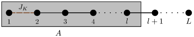
Figure 1: An example of a spin chain with only nearest-neighbour-interactions and an impurity on the first site. The interactions of the impurity site are multiplied by a $J_{K}$. The chain is separated into part $A$ (grey box), which includes the impurity and has the length $l$, and the rest of the chain.

Based on this observation, the impurity entanglement-entropy $S_{\mathrm{imp}}(J_{K},l,L)$ was introduced to quantify the contribution an impurity has to the entanglement of a spin chain [9, 10]. To model an impurity, the interactions on one site are scaled by a factor of $J_{K}$. The impurity entanglement-entropy is given by the difference of the uniform part of the entanglement-entropies of the chain with the impurity present and the chain without the impurity. The sub-system $A$ in the definition of the entanglement-entropy in equation 1 is chosen to contain the first $l$ sites of the chain and thus contains the impurity site, too (see figure 1). Upon removing the impurity site, $A$ as well as the whole chain are one element shorter. The uniform entanglement-entropy in a system where the impurity is absent is thus given by $S_{u}(1,l-1,L-1)$. This leads to the following definition of $S_{\mathrm{imp}}$:

$$S_{\mathrm{imp}}(J_{K},l,L) \equiv S_{u}({\rm with\ impurity})-S_{u}({\rm no\ impurity})$$ (3)

$$\equiv S_{u}(J_{K},l,L)-S_{u}(1,l-1,L-1),\ l>1\ .$$

This definition is similar in spirit to experimental procedures for extracting impurity contributions to, for instance, susceptibilities. It is also possible to consider the alternating part of the impurity entanglement but we shall not do that here.

However, it was later pointed out [11, 12] that a more consistent definition of the impurity contribution to the entanglement can be obtained from the negativity [26]. The negativity between a sub-system $A$ and the rest of the system is defined by

$$\mathcal{N}=\frac{\sum|\lambda_{i}|-1}{2}\ ,$$ (4)

where the $\lambda_{i}$ are the eigenvalues of the partial transpose of the density-matrix with respect to either $A$ or the rest of the system. In contrast to the entanglement-entropy it can also be used to quantify the entanglement if the system is not in a pure state. This makes it possible to use the negativity to directly quantify the entanglement of the impurity-spin and another part of the system.

It is an important question to what extent these two quantities yield the same information about the impurity entanglement. In this paper we compare these two measures and show that they agree for many universal features but are fundamentally different with $\mathcal{N}$ being the more general measure of the impurity entanglement.

Entanglement and in particular impurity entanglement in gapped quantum spin chains has received comparatively little attention. In part this is due to the fact that for non-critical spin chains with a finite correlation length $\xi$ one expects [1] for a partition into 2 semi-infinite chains:

$$S\sim\log{\xi}\ .$$ (5)

For instance, for the $S=1$ Affleck-Kennedy-Lieb-Tasaki (AKLT) chain [27, 28] where the entanglement can be calculated analytically  [29, 30, 31, 32, 33, 34, 35] it is known that $S(l,L)$ approaches a constant for large $l,L$ in an exponential manner [34, 35] on a length scale equal to the bulk correlation length $\xi=1/\ln(3)$. At the Majumdar-Ghosh-point (MG-point) [36] of the $J-J_{2}$ spin chain, where $J_{2}=J/2$, one finds that $S(l,L)$ is either 0 or $\ln(2)$ for any $l,L$. However, the impurity contribution to the entanglement can still be long-range in gapped spin chains. For the $J-J_{2}$ spin chain this was shown to be the case at the MG-point [9, 10]. This is due to the two-fold degeneracy of the singlet ground-state, corresponding to the two different dimerization patterns, and the associated presence of solitons separating regions with different dimerization. The model we study is the slightly more general $J-J_{2}-\delta$ quantum spin chain defined as:

$$H= J_{K}\Big{[}(1+\delta)\vec{S}_{0}\cdot\vec{S}_{1}+J_{2}\;\vec{S}_{0}\cdot\vec{S}_{2}\Big{]}$$ (6)

$$+\sum_{i=1}^{L-3}\Big{[}(1+(-\delta)^{i})\vec{S}_{i}\cdot\vec{S}_{i+1}+J_{2}\;\vec{S}_{i}\cdot\vec{S}_{i+2}\Big{]}$$

$$+(1+(-\delta)^{L-2})\vec{S}_{L-2}\cdot\vec{S}_{L-1}\;,$$

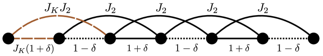
Figure 2: The $J-J_{2}-\delta$ chain with an impurity coupled with strength $J_{K}$.

where we implicitly have set the nearest-neighbour-coupling $J\equiv 1$. The coefficient $J_{K}$ describes the coupling of the impurity-spin and $\delta$ is a staggering of the nearest-neighbour-coupling inducing dimerization. We focus exclusively on chains with open boundary conditions and the impurity at one end of the chain. With $\delta=0$ this model undergoes a transition from the gapless Heisenberg-phase to a dimerized state at $J_{2}^{c}=0.241167$ [37, 38]. In the Heisenberg-phase a correspondence to the low-energy physics of a Kondo impurity can be established [39, 40]. This correspondence becomes exact at $J_{2}^{c}$. The mapping to the Kondo-problem requires one to use open boundary conditions and we therefore do not consider periodic boundary conditions here. However, entanglement in models similar to the one considered here but with periodic boundary conditions have also been studied, see section 4 of Ref. [14] for a review.

With periodic boundary conditions and an even number of sites, the system at the MG-point has an exactly known two-fold degenerate dimerized ground-state and a gapped spectrum [36, 41]. (With open boundary conditions and $L$ even the ground-state is unique with the same energy). The lowest lying excitations of the MG-chain are pairs of unbound solitons and upon introducing a finite dimerization the solitons become confined [42]. For a chain with an odd number of sites solitons separate regions with the ground-state dimerization-pattern of the chain with an even number of sites [41, 42]. In the gapped phase, in the proximity of the MG-point, it is possible to perform very precise variational calculations [41, 43, 44] for the $J-J_{2}$ model (corresponding to $\delta=0$ in this study) since appropriate states spanning the variational sub-space can be identified with relative ease, as the ground-state at the MG-point is known. Within this variational framework it is possible to evaluate the entanglement [10]. Here, we explain in detail how similar calculations can be performed for the negativity and discuss the appropriate sub-spaces used in these computations. Along the so called disorder-line, where $J_{2}=(1-\delta)/2$, one of the two degenerate ground-states of the Majumdar-Ghosh-chain remains the exact ground-state. Close to the disorder-line, one therefore expects the same variational methods to yield very precise results.

In the past, these variational calculations have been performed more or less by hand [41, 43, 44]. If the variational problem is, however, formulated as a generalized eigenvalue-problem, it is not difficult to automate the calculation, as for any two states, $\varphi_{i}$ and $\varphi_{j},$ with all but no, one or two sites being in dimers, $\langle\varphi_{i}|\vec{S}_{i}\vec{S}_{j}|\varphi_{j}\rangle$ as well as the overlaps between different $\varphi$ can be computed in an automated fashion. One advantage of the automated computation of these matrix-elements is that one avoids lengthy and error-prone calculations. Secondly, solving a generalized eigenvalue-problem can be done using standard libraries. This approach is not limited to the specific Hamiltonian studied in this paper. It can in fact be used to perform variational calculations using dimerized states forming the subspace in which the diagonalization is carried out for any Heisenberg-spin-Hamiltonian.

In addition to providing a more direct analytical insight into the physics, the main advantages the variational approach has over other methods such as the DMRG-technique are computational cost and simplicity. This advantage does, however, not come for free. To identify a good subspace to use for variational calculations, one always has to rely on knowledge gained obtained by other means. This role is often played by the DMRG-technique.

The paper is organized as follows: In sections 2, 3, 4 and 5 the variational approach is discussed along with the different sub-spaces used in the calculations. Section 6 describes the calculation of the negativity once the variational ground-state is known and sample results for the negativity are compared to DMRG-data. In section 7 the negativity and the impurity-entanglement-entropy are compared. Section 8 presents our results for the negativity and $S_{\mathrm{imp}}$ for general $J_{K}$ at the MG point. In section 9 we describe how the impurity entanglement is affected by the presence of a non-zero explicit dimerization, $\delta$.

2 The Variational Calculation as a Generalized Eigenvalue-Problem

For completeness we review here how the variational problem can be formulated as a generalized eigenvalue-problem. Consider a set of states $\{\varphi_{i}\}$ to be used for the variational calculation. We then wish to minimize

$$\langle H\rangle=\frac{(\varphi|H\varphi)}{(\varphi|\varphi)}\ ,$$ (7)

where the trial-state $\varphi$ is given by:

$$\varphi=\sum c_{j}\varphi_{j}\ .$$ (8)

The minimization is to be performed with respect to the $c_{j}$. In variational calculations we make use of the fact that:

$$\forall\varphi:\ E_{0} \leq\frac{(\varphi|H\varphi)}{(\varphi|\varphi)}\ ,$$ (9)

where $E_{0}$ is the ground-state energy. One strives to find a well chosen set of $\varphi_{i}$s as well as the state $\varphi_{min}\in\mathrm{span}\{\varphi_{i}\}$ that satisfies

$$\frac{(\varphi|H\varphi)}{(\varphi|\varphi)}\Big{|}_{\varphi_{min}} =\mathrm{min}_{\mathrm{span}\{\varphi_{i}\}}{\frac{(\varphi|H\varphi)}{(\varphi|\varphi)}}\ .$$ (10)

This state is the variational estimate for the ground-state. Let us denote the energy-eigenbasis with $\{\mathfrak{e}_{i}\}$. The variational state $\varphi$ can evidently be written as $\varphi=\sum a_{i}\mathfrak{e}_{i}$. Thus

$$\frac{(\varphi|H\varphi)}{(\varphi|\varphi)} =\sum_{i,j}\bar{a}_{i}a_{j}\frac{(\mathfrak{e}_{i}|H\mathfrak{e}_{j})}{\sum_{i}|a_{i}|^{2}}$$ (11)

$$=\frac{\sum_{i}|a_{i}|^{2}E_{i}}{\sum_{i}|a_{i}|^{2}}$$

$$\geq E_{v}\ ,$$

where $E_{v}$ is the energy of the eigenstate $\mathfrak{e}_{v}$ of non-zero projection onto $\mathrm{span}\left\{\varphi_{i}\right\}$ that has the lowest energy. With any orthonormal basis $\{\mathfrak{b}_{i}\}$ of $\mathrm{span}\{\varphi_{i}\}$, the variational guess for the ground-state $\varphi_{min}$ can thus be found by diagonalizing $H$:

• Minimization problem $\equiv$ Finding lowest eigenvalue of $\big{(}\mathfrak{b}_{i}|H\mathfrak{b}_{j}\big{)}$

If we do not have an orthonormal basis at our disposal, we have to do a little more work. Let us suppose that the $\varphi_{i}$ are linearly independent and the $\mathfrak{e}_{i}$ are the orthonormal basis of energy-eigenstates. For the variational ground-state given by $\varphi_{min}=\sum_{i}a_{i}\varphi_{i}$ and the variational estimate of the ground-state-energy $E_{v}$ we know from the equations (11) that

$$H\sum_{j}a_{j}\varphi_{j} =E_{v}\sum_{j}a_{j}\varphi_{j}\ .$$ (12)

We will now show that a vector $\mathfrak{a}=(a_{1},\dots,a_{n})$ is a solution to the variational problem if and only if

$$\forall i:\;\;\sum_{j}a_{j}(\varphi_{i}|H\varphi_{j})=E_{v}\sum_{j}a_{j}(\varphi_{i}|\varphi_{j})\ .$$ (13)

With the definitions

$$\mathfrak{H}_{ij}=\big{(}\varphi_{i}\big{|}H\varphi_{j}\big{)}\phantom{undoder}\mathrm{and}\phantom{undoder}\mathfrak{B}_{ij}=\big{(}\varphi_{i}\big{|}\varphi_{j}\big{)}\ ,$$ (14)

one can write equation (13) as

$$\mathfrak{H}\mathfrak{a}=E_{v}\mathfrak{B}\mathfrak{a}\ ,$$ (15)

which defines a generalized eigenvalue-problem. That equation (12) implies equation (13) can be seen by taking the scalar-product of both sides in equation (12) with $\varphi_{i}$.

That equation (13) implies (12) will now be proved. We do this by proving that for any basis (linearly independent set of states that span the space) $\{\varphi_{i}\}$:

$$\forall i:\;\;(\varphi_{i}|\mathfrak{q})=(\varphi_{i}|\mathfrak{r})\;\;\;\Rightarrow\;\;\;\mathfrak{q}=\mathfrak{r}\ ,$$ (16)

for any vectors $\mathfrak{q}$, $\mathfrak{r}$. With $\mathfrak{q}=H\sum_{j}a_{j}\varphi_{j}$ and $\mathfrak{r}=E_{v}\sum_{j}a_{j}\varphi_{j}$ the relation (16) becomes the relation equation (13) $\Rightarrow$ (12).

Proof:

$$\forall i:\;\;(\varphi_{i}|\mathfrak{q})=(\varphi_{i}|\mathfrak{r})$$ (17)

$$\Rightarrow$$ (18)

$$\forall i:\;\;(\varphi_{i}|\mathfrak{q}-\mathfrak{r})=0$$

$$\Rightarrow$$ (19)

$$\forall i:\;\;\varphi_{i}\bot(\mathfrak{q}-\mathfrak{r})$$

$$\Rightarrow$$ (20)

$$\phantom{\forall i:\;\;}\mathfrak{q}-\mathfrak{r}=0\phantom{Beweisbeended}\Box$$

We have thus proven that the minimization-problem of equation (10) can be replaced by the generalized eigenvalue-problem of equation (15), if the states used to span the subspace in which the minimization takes place are linearly independent.

3 The Hilbert Spaces Used in the Calculation

The implementation of the variational technique as a generalized eigenvalue-problem allows us to just solve a linear algebra problem instead of solving a set of non-linear equations which is necessary if one approaches the minimization naively. The one requirement for this implementation to work is for the states that span the Hilbert-space in which the minimization is done to be linearly independent. This flexibility makes it possible to use different bases according to the specific needs of the problem. Here we are concerned with the two cases of even and odd length chains.

1. Chain with odd number of sites:
   The simplest ensemble of variational states for a chain with an odd number of sites are the so called single soliton states [41, 43, 44, 10]. These states can be generated by taking $L-1$ of the sites of the chain to be maximally dimerized while leaving the left over site (the soliton) to be in the $S_{z}=1/2$ state. Here and in the remainder of the paper we use $L$ to denote the length of the chain. The number of dimers between the undimerized site and the left end of the chain can be used to label the states. In figure 3 we show a pictorial representation of the first three states. When drawing a dimer we use an arrow to denote the order in $(|\uparrow\downarrow\rangle-|\downarrow\uparrow\rangle)/\sqrt{2}$. For an odd length chain with $L$ spins there exist $N=(L+1)/2$ such states. Note that we here do not include states with the soliton in the $S_{z}=-1/2$ state.

   

   (a) $\varphi_{0}$

   

   (b) $\varphi_{1}$

   

   (c) $\varphi_{2}$

   Figure 3: The first three variational states used in the calculations with the single soliton space for a chain with an odd number of sites. Note the arrows on the dimers that indicate their direction.

2. Chain with even number of sites:
   In studies of the entanglement of the impurity-site with the rest of a chain with an even number of sites, a suitable set of states can be defined by leaving the bulk $(L-2)$ sites of the chain dimerized while one of the spins is in a valence bond with the impurity. Example-states are given in figure 4.

   

   (a) $\varphi_{0}$

   

   (b) $\varphi_{1}$

   

   (c) $\varphi_{2}$

   Figure 4: The first three variational states used in the calculation of the negativity for a chain with an even number of sites.

   These states are chosen in order to reflect the presence of an impurity valence bond (IVB) [10], connecting the impurity site to the bulk of the chain.

4 The Matrix Elements of of the Hamiltonian $\mathfrak{H}$

To set up the generalized eigenvalue-problem it is necessary to calculate the matrices $\mathfrak{H}$ and $\mathfrak{B}$ which were defined in equation (14). In this section we will explain how to compute $\mathfrak{H}$. In order to allow for the most general Hamiltonian possible we write it as follows:

$$H=\sum_{\{m,l\}}J_{ml}\vec{S}_{m}\vec{S}_{l}\ .$$ (21)

Here, the summation $\{m,l\}$ is over ’bonds’ of the Hamiltonian and the coupling constants $J_{ml}$ can take any value. It is convenient to write the matrix-elements $\mathfrak{H}_{ij}$ in terms of the operators $h_{ml}=\vec{S}_{m}\vec{S}_{l}-1/4$, because they have a simple action on the $\varphi$s. This gives:

$$\big{(}\varphi_{i}\big{|}H\varphi_{j}\big{)} =\sum_{\{m,l\}}J_{ml}\big{(}\varphi_{i}\big{|}\vec{S}_{m}\vec{S}_{l}\varphi_{j}\big{)}$$ (22)

$$=\sum_{\{m,l\}}J_{ml}\big{(}\varphi_{i}\big{|}\big{[}h_{ml}+1/4\big{]}\varphi_{j}\big{)}\ ,$$

The following description of this action is an extension of results presented earlier [45] in the context of quantum Monte Carlo simulations in the valence bond basis where it is necessary to take the $h_{ml}$ to have the opposite sign of what we use here. The action of $h_{ml}$ on states relevant to us is given by:

$$h_{ml}\big{[}m;l\big{]}\big{[}k;n\big{]} =-\big{[}m;l\big{]}\big{[}k;n\big{]}$$ (23)

$$h_{mk}\big{[}m;l\big{]}\big{[}k;n\big{]} =\frac{1}{2}\big{[}m;k\big{]}\big{[}n;l\big{]}$$ (24)

$$h_{ml}\uparrow_{m}\big{[}l;k\big{]} =\frac{1}{2}\big{[}m;l\big{]}\uparrow_{k}$$ (25)

$$h_{mk}\big{[}m;l\big{]}\uparrow_{k} =-\frac{1}{2}\Big{[}\uparrow_{m}\big{[}l;k\big{]}+\big{[}m;l\big{]}\uparrow_{k}\Big{]}\ ,$$ (26)

where

$$\big{[}m;k\big{]} :=\frac{1}{\sqrt{2}}\big{(}\uparrow_{m}\downarrow_{k}-\uparrow_{k}\downarrow_{m}\big{)}$$

are the spins at $m$ and $k$ in a singlet-state.

In figure 5 a pictorial representation of the equations (23)-(26) is shown. To fix the phase of the states we include in the calculation, we again represent $\big{[}m;k\big{]}$ by an arrow pointing from $m$ to $k$.

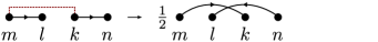
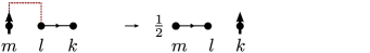
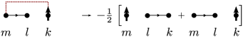
Figure 5: The action of $h_{ml}$ on the variational states. The dotted line signifies the sites acted upon by $h_{ml}$. Arrows fix the phase of singlets between sites of the lattice. The convention is explained in the main text.

For the calculations we present here these are the only rules needed. However, when considering the action of the Hamiltonian it is sometimes convenient to apply the simple rules

$$\big{[}m;k\big{]} =-\big{[}k;m\big{]}$$ (27)

$$\big{[}k;l\big{]}\uparrow_{m} =\big{[}k;m\big{]}\uparrow_{l}+\uparrow_{k}\big{[}m;l\big{]}\ ,$$ (28)

in order to reduce the action of the $h_{ml}$ to one of the above.

We want to stress that even though the single soliton states can be orthogonalized with relative ease [46] this is not generally the case and even after orthogonalization the resulting eigenvalue problem is still non-trivial for a general set of $J_{lm}$. Whether or not it is possible to proceed with analytical calculations often depends on specific choices for the coupling constants in the Hamiltonian. Here, we can solve the variational problem for any values of the couplings.

As can be seen in equation (24) and figure 5(b), the application of $h_{ml}$ to a given state $\varphi_{i}$ may result in a state that is not element of $\mathrm{span}\{\varphi_{i}\}$. Therefore, in order to evaluate

$$\big{(}\varphi_{i}\big{|}H\varphi_{j}\big{)} =\sum_{\{m,l\}}J_{ml}\big{(}\varphi_{i}\big{|}h_{ml}\varphi_{j}\big{)}$$

we need to compute the overlap of $h_{ml}\varphi_{j}$ with all the variational states. This slows down our calculations since it is not sufficient to build a table of all the overlaps of the $\varphi_{i}$. We now turn to a discussion of how the overlaps are calculated.

5 The Matrix Elements of the Overlap-Matrix $\mathfrak{B}$

As is explained in [47, 45] the magnitude of the overlaps of valence-bond-states depends solely on the length of loops created by overlaying the two states. If one chooses $l$ to be the length of such a loop then the overlap is of magnitude $2^{-l/2+1}$. To get the sign of the overlap we, in addition to overlaying them, reverse all arrows on one of the states. Then we follow the loop and count how often one has to go against the arrow. If the resulting number is odd, the sign of the overlap is negative. If the resulting number is even, the sign of the overlap is positive. Because the total number of bonds in the loop is even this leads to a well defined sign of the overlap.

Figure 6: The two states (a) and (b) together with the corresponding loop-structure created by reversing the arrows of one state and overlaying the two states (c). Both loops contribute a minus-sign. The overlap is given by $1/4$.

To get the overlaps of two states one only has to follow this prescription for every loop and multiply contributions from different loops. Figure 6(c) shows the loop-structure for the states shown in figure 6(a) and figure 6(b). The left loop is six bonds long and going around it one has to go against the direction of the arrow three times. The right loop is 2 bonds long and one has to go against the direction of the arrow once. The overlap is therefore given by:

$$(-2^{-2})(-2^{0})=\frac{1}{4}\ .$$

In the case of unpaired spins being part of the states the rules have to be modified slightly. If there is one unpaired spin in both states, upon overlaying the two states, there will in addition to loops be a string that goes from one unpaired spin to the other. As is the case for the loops, for the string the magnitude of the contribution to the overlap depends only on the length. One finds the contribution to be: $2^{-l/2}$. The contribution to the sign of the overlap can be determined in exactly the same way as in the case of complete loops.

6 The Calculation of the Reduced Density-Matrix and the Negativity

For the calculation of the negativity describing the entanglement between the impurity-spin and a distant part of the chain, it is necessary to separate the chain into three parts [26, 11]: the impurity-spin, the part whose entanglement with the impurity-spin is to be quantified and the part that separates the two (the parts will in the remainder of the paper also be referred to as region a, b and x respectively. The negativity is invariant under interchange of b and x. For clarification see figure 7).

Figure 7: The chain separated into three parts: the impurity-spin (a), the part whose entanglement with the impurity-spin is to be quantified (b) and the part that separates the two (x).

To calculate the negativity between the impurity-spin and a part of the chain that is separated from the impurity-spin by a different part, we have to compute the reduced density-matrix that results from tracing out the separating part of the chain. We will now explain how this is done within our variational framework.

Let the result of the generalized eigenvalue problem be the variational ground-state $\varphi_{g}$ given in the variational basis: $\varphi_{g}=\sum a_{i}\varphi_{i}$. To take trace of the density-matrix over the region x in figure 7, we express the density-matrix in a product-basis formed by states of region x and states of the rest of the chain. This requires us to represent the variational ground-state $\varphi_{g}$ in this product-basis. In doing so we follow the approach of reference [10], where the entanglement-entropy was calculated from a variational ground-state. For a chain with an odd number of spins these bases will in the following be introduced. We start with the case that the region x contains an even number of sites followed by the case that the region x contains an odd number of sites. For a chain with an even total number of sites an analogous calculation was performed.

6.1 An even number of sites to be traced out

1. For the impurity-spin we choose the $S_{z}$-basis and denote the two states by $f_{1}=\,\uparrow$ and $f_{2}=\,\downarrow$ .

2. For the region x we denote the basis by ${g_{i}}$. We take the region to contain at least two sites. The states are chosen to be:

   $$g_{1}= \sum_{n=1}^{R}a_{n}\ \underbrace{\uparrow\ \overbrace{\ \relbar\phantom{\uparrow}\dots\phantom{\uparrow}\relbar\ }^{n-1\ \mathrm{dimers}}\ \uparrow\ \relbar\ \dots\ \relbar}_{2R\ \mathrm{sites}}\ ,$$

   $$g_{2}= \sum_{n=1}^{R}a_{n}\ \underbrace{\uparrow\ \overbrace{\ \relbar\phantom{\uparrow}\dots\phantom{\uparrow}\relbar\ }^{n-1\ \mathrm{dimers}}\ \downarrow\ \relbar\ \dots\ \relbar}_{2R\ \mathrm{sites}}\ ,$$

   $$g_{3}= \underbrace{\uparrow\ \relbar\ \dots\ \relbar\uparrow}_{2R\ \mathrm{sites}}\ ,\ \ g_{4}=\underbrace{\downarrow\ \relbar\ \dots\ \relbar\downarrow}_{2R\ \mathrm{sites}}\ ,$$

   $$g_{5}= \underbrace{\downarrow\ \relbar\ \dots\ \relbar\uparrow}_{2R\ \mathrm{sites}}\ ,\ \ g_{6}=\underbrace{\uparrow\ \relbar\ \dots\ \relbar\downarrow}_{2R\ \mathrm{sites}}\ ,$$

   $$g_{7}= \underbrace{\relbar\ \dots\ \relbar}_{2R\ \mathrm{sites}}\ ,$$

   where the symbol ’$\relbar$’ is used for valence-bonds between neighbouring sites and $R$ is the highest possible number of dimers that can could be formed in region x.

3. For region b we define the states in the following way:

   $$\tilde{h}_{1}= \underbrace{\relbar\ \dots\ \relbar}_{L-2R-1\ \mathrm{sites}}$$

   $$\tilde{h}_{2}= \sum_{n=R+1}^{N-1}a_{n}\ \underbrace{\uparrow\ \overbrace{\ \relbar\phantom{\uparrow}\dots\phantom{\uparrow}\relbar\ }^{n-R-1\ \mathrm{dimers}}\ \uparrow\ \relbar\ \dots\ \relbar}_{L-2R-1\ \mathrm{sites}}$$

   $$\tilde{h}_{3}= \sum_{n=R+1}^{N-1}a_{n}\ \underbrace{\downarrow\ \overbrace{\ \relbar\phantom{\uparrow}\dots\phantom{\uparrow}\relbar\ }^{n-R-1\ \mathrm{dimers}}\ \uparrow\ \relbar\ \dots\ \relbar}_{L-2R-1\ \mathrm{sites}}$$

   In order to express the density-matrix of the impurity-spin and the region b in an orthonormal basis it is necessary to orthonormalize the basis $\{\tilde{h}_{i}\}$ as it is not orthogonal the way it is defined above:

   $$(\tilde{h}_{1}|\tilde{h}_{3})=\sum_{n=R+1}^{N-1}a_{n}\ (-2)^{-n+R+1}\left(\frac{-1}{\sqrt{2}}\right)\ .$$ (29)

   We do this following the usual Gram-Schmidt procedure. Our orthonormalized version is given by:

   $$h_{1} =\frac{\tilde{h}_{1}}{\sqrt{(\tilde{h}_{1}|\tilde{h}_{1})}}$$

   $$h_{2} =\frac{\tilde{h}_{2}}{\sqrt{(\tilde{h}_{2}|\tilde{h}_{2})}}$$

   $$h_{3} =\frac{\tilde{h}_{3}-(\tilde{h}_{3}|h_{1})h_{1}}{\sqrt{(\tilde{h}_{3}|\tilde{h}_{3})-|(\tilde{h}_{3}|h_{1})|^{2}}}\ .$$ (30)

For the product-space of the impurity-spin and region b we use the basis-states:

$$k_{1} =f_{1}h_{1},\ k_{2}=f_{1}h_{2},\ k_{3}=f_{1}h_{3},\$$

$$k_{4} =f_{2}h_{1},\ k_{5}=f_{2}h_{2},\ k_{6}=f_{2}h_{3}\ .$$

With these definitions, the variational ground-state can be written as:

$$\varphi_{g}=\sum a_{n}\varphi_{n}=\sum_{i,j}C_{ij}k_{i}g_{j}\ ,$$ (31)

where the matrix $C$ is given by:

$$C=\left(\begin{array}[]{ccccccc}0&\frac{\|\tilde{h}_{1}\|}{\sqrt{2}}&0&0&0&\frac{(\tilde{h}_{3}|h_{1})}{2}&a_{0}\|\tilde{h}_{1}\|\\ 0&0&0&-\frac{\|\tilde{h}_{2}\|}{\sqrt{2}}&0&0&0\\ 0&0&0&0&\frac{\kappa}{2}&0&0\\ -\frac{\|\tilde{h}_{1}\|}{\sqrt{2}}&0&-\frac{(\tilde{h}_{3}|h_{1})}{2}&0&0&0&0\\ 0&0&0&0&0&-\frac{\|\tilde{h}_{2}\|}{2}&0\\ 0&0&-\frac{\kappa}{2}&0&0&0&0\\ \end{array}\right)\ ,$$ (38)

where $\kappa=\sqrt{\|\tilde{h}_{3}\|^{2}-|(\tilde{h}_{3}|h_{1})|^{2}}$ and $\|h\|=\sqrt{(h|h)}$.

With the matrix $G_{ij}:=(g_{i}|g_{j})$, whose matrix-elements can be computed using the prescription given in section 5, one can write the reduced density-matrix of the impurity-spin and region b as

$$(\rho_{ab})_{ij} =(\mathrm{tr}_{x}\ \rho_{axb})_{ij}$$ (39)

$$=\sum_{n,m}C_{in}C_{jm}(g_{n}|g_{m})\ ,$$

or in matrix form:

$$\rho_{ab} =CGC^{\mathrm{T}}\ .$$ (40)

6.2 An odd number of sites to be traced out

1. For the impurity-spin we choose the $S_{z}$-basis and denoted the two states by $f_{1}=\,\uparrow$ and $f_{2}=\,\downarrow$ .

2. For the region to be traced out we denote the basis by ${g_{i}}$. The states are chosen to be:

   $$g_{1}= \underbrace{\relbar\ \dots\ \relbar\downarrow}_{2R+1\ \mathrm{sites}}\ ,\ \ g_{2}=\underbrace{\relbar\ \dots\ \relbar\downarrow}_{2R+1\ \mathrm{sites}}\ ,$$

   $$g_{3}= \sum_{n=1}^{R}a_{n}\ \underbrace{\uparrow\ \overbrace{\ \relbar\phantom{\uparrow}\dots\phantom{\uparrow}\relbar\ }^{n-1\ \mathrm{dimers}}\ \uparrow\ \relbar\ \dots\ \relbar\uparrow}_{2R+1\ \mathrm{sites}}\ ,$$

   $$g_{4}= \sum_{n=1}^{R}a_{n}\ \underbrace{\downarrow\ \overbrace{\ \relbar\phantom{\uparrow}\dots\phantom{\uparrow}\relbar\ }^{n-1\ \mathrm{dimers}}\ \uparrow\ \relbar\ \dots\ \relbar\uparrow}_{2R+1\ \mathrm{sites}}\ ,$$

   $$g_{5}= \sum_{n=1}^{R}a_{n}\ \underbrace{\uparrow\ \overbrace{\ \relbar\phantom{\uparrow}\dots\phantom{\uparrow}\relbar\ }^{n-1\ \mathrm{dimers}}\ \uparrow\ \relbar\ \dots\ \relbar\downarrow}_{2R+1\ \mathrm{sites}}\ ,$$

   $$g_{6}= \sum_{n=1}^{R}a_{n}\ \underbrace{\downarrow\ \overbrace{\ \relbar\phantom{\uparrow}\dots\phantom{\uparrow}\relbar\ }^{n-1\ \mathrm{dimers}}\ \uparrow\ \relbar\ \dots\ \relbar\downarrow}_{2R+1\ \mathrm{sites}}\ ,$$

   $$g_{7}= \underbrace{\uparrow\relbar\ \dots\ \relbar}_{2R+1\ \mathrm{sites}}\ ,\ \ g_{8}=\underbrace{\downarrow\relbar\ \dots\ \relbar}_{2R+1\ \mathrm{sites}}\ ,$$

   where the symbol ’$\relbar$’ is used for valence-bonds between neighbouring sites and $R$ is the highest possible number of dimers that can could be formed in region x.

3. For region b we define the states in the following way:

   $$\tilde{h}_{1}= \underbrace{\uparrow\relbar\ \dots\ \relbar}_{L-2R-2\ \mathrm{sites}}\ ,\ \ \tilde{h}_{2}=\underbrace{\downarrow\relbar\ \dots\ \relbar}_{L-2R-2\ \mathrm{sites}}\ ,$$

   $$\tilde{h}_{3}= \sum_{n=R+1}^{N-1}a_{n}\ \underbrace{\overbrace{\ \relbar\phantom{\uparrow}\dots\phantom{\uparrow}\relbar\ }^{n-R-1\ \mathrm{dimers}}\ \uparrow\ \relbar\ \dots\ \relbar}_{L-2R-2\ \mathrm{sites}}\ .$$

   We orthonormalize and build a product-basis for the impurity-spin and region b just as it is done in the case of an even number of sites that have to be traced out.

With $G_{ij}:=(g_{i}|g_{j})$ and

$$C=\left(\begin{array}[]{cccccccc}-\frac{a_{0}}{\sqrt{2}}&0&0&0&0&-\frac{1}{2}&0&\frac{(\tilde{h}_{1}|\tilde{h}_{3})}{\sqrt{2}}\\ 0&\frac{a_{0}}{\sqrt{2}}&0&\frac{1}{2}&0&0&0&0\\ 0&0&0&0&0&0&0&\frac{\kappa}{\sqrt{2}}\\ 0&0&0&0&\frac{1}{2}&0&-\frac{(\tilde{h}_{1}|\tilde{h}_{3})}{\sqrt{2}}&0\\ 0&0&-\frac{1}{2}&0&0&0&0&0\\ 0&0&0&0&0&0&-\frac{\kappa}{\sqrt{2}}&0\\ \end{array}\right)\ ,$$ (47)

where $\kappa=\sqrt{(\tilde{h}_{3}|\tilde{h}_{3})-|(\tilde{h}_{3}|h_{1})|^{2}}$, we can again write the reduced density-matrix as

$$\rho_{ab} =CGC^{\mathrm{T}}\ .$$ (48)

For a chain with an even total number of sites we followed an analogous procedure. In order to save space we have not included it here.

6.3 The Negativity

With the expression for the reduced density-matrix of the impurity-spin and region b, $\rho_{ab}$, at hand it is now straight forward to calculate the negativity according to its definition [26]

$$\mathcal{N}=\frac{\sum|\lambda_{i}|-1}{2}\ ,$$ (49)

where the $\lambda_{i}$ are the eigenvalues of the partial transpose of $\rho_{ab}$.

6.4 Precision of the Variational Approach

The variational states that form our starting point should yield almost exact results close to the MG-point ($J_{2}=J/2$) where a chain with an even number of spins is fully dimerized. However, the states we include in our variational calculation (see section 3) form only a subset of the states in which the bulk of the chain is dimerized. At the MG-point the contribution arising from these neglected states is negligible and the variational approach is very good. However, as $J_{2}$ is decreased toward the critical point $J_{2}^{c}$ we expect the contribution from the neglected states to grow in importance and at $J_{2}^{c}$, where the ground-state is no longer dimerized, we expect our variational approach to fail. Nevertheless, for intermediate $J_{2}$, $J_{2}^{c}<J_{2}\leq J/2$ we still expect the variational approach to yield qualitatively good results.

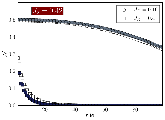
Figure 8: Variational results for the negativity (filled symbols) together with DMRG-data from reference [11] (empty symbols) for two values of the impurity-coupling $J_{K}$. The calculations were done for a chain of length $L=250$, with frustration $J_{2}=0.42$ and dimerization $\delta=0$.

It is possible to calculate the negativity, $\mathcal{N}$, using DMRG techniques, as was shown by Bayat et al [11]. In figure 8 we compare our variational results for $\mathcal{N}$ to DMRG results from reference [11] at $J_{2}=0.42J$ for 2 different values of $J_{K}$: $J_{K}=0.16$ and $J_{K}=0.4$ (Here $\delta=0$). The definition of $\mathcal{N}$ used in reference [11] differs from the one used by us by a factor of two. To account for this difference we multiplied their data by two. For both values of $J_{K}$ we observe a very good agreement between the DMRG and variational results.

7 $\mathcal{N}$ Compared to $S_{\mathrm{imp}}$ at the MG-Point

Having established the validity of the variational approach we now turn to a comparison of the two measures for the impurity entanglement $\mathcal{N}$ [11] and $S_{\mathrm{imp}}$ [9]. In figure 9 we show results for both $\mathcal{N}$ and $S_{\mathrm{imp}}$ at the MG-point for a system with $L=200$ sites and an impurity-coupling $J_{K}=0$. Shown is also the impurity entanglement arising from a single impurity valence bond (IVB) [9] between the impurity-spin and the bulk of the chain.

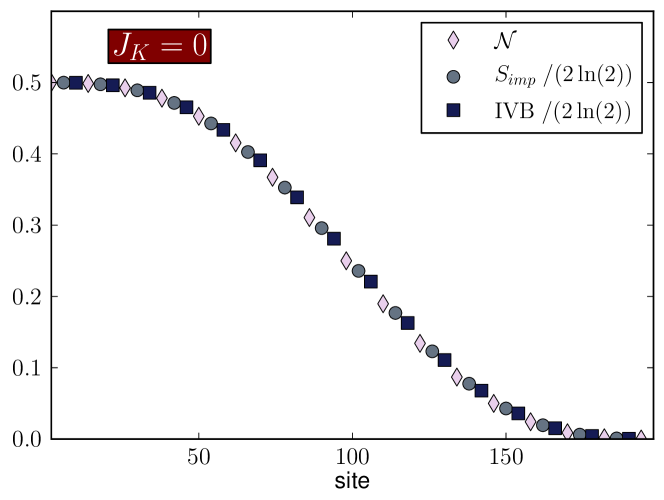
Figure 9: Variational results for the negativity $\mathcal{N}$ and the impurity entanglement $S_{imp}$ scaled by $1/(2\mathrm{ln}(2))$ at impurity-coupling $J_{K}=0$ and $\delta=0$. Shown is also the impurity entanglement arising from an impurity valence bond (IVB) scaled by $1/(2\mathrm{ln}(2))$. The calculations were done for a chain of length $L=200$ at the MG-point. For clarity only a fraction of all data points are shown.

For $J_{K}=0$ and $L$ even, the idea of an impurity valence bond is easy to understand. The uncoupled impurity must form a singlet with the unpaired $S=1/2$ in the bulk of the chain. If the entire system (impurity and bulk) is divided in 2 parts $A$ and $B$ this impurity valence bond will contribute either $\ln(2)$ or $0$ depending on whether the unpaired spin is in part $B$ or $A$. With the wave-function for the unpaired spin $\varphi_{\mathrm{sol}}(x)$ and $p=\int_{A}|\varphi_{\mathrm{sol}}(x)|^{2}dx$, the impurity entanglement is then simply [9, 10]:

$$S_{\mathrm{imp}}^{\mathrm{IVB}}=(1-p)\ln(2).$$ (50)

To a first approximation $\varphi_{\mathrm{sol}}(x)$ can be taken to be the wave-function of a free particle in a box [10]:

$$\varphi_{\mathrm{sol}}(i)=\sqrt{\frac{2}{L}}\mathrm{sin}\left(\frac{\pi i}{L}\right)\ .$$ (51)

It is also possible to obtain more precise estimates of $\varphi_{\mathrm{sol}}$ [10]. Apart from an overall scaling factor of $2\ln(2)$ the two measures are in the case shown in figure 9 essentially identical.

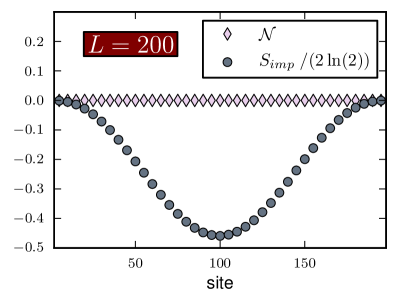
(a) $L=200$

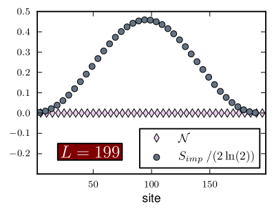
(b) $L=199$

Figure 10: Variational results for the negativity $\mathcal{N}$ and the impurity entanglement $S_{imp}$ scaled by $1/(2\mathrm{ln}(2))$ at impurity-coupling $J_{K}=1$. The calculations were done at the MG-point for a chain of length $L=200$ (a) as well as $L=199$ (b). For clarity only a fraction of all data points are shown.

We now compare the two measures of the impurity entanglement in the limit $J_{K}=1$. In figure 10(a) we show variational results for both quantities at $J_{K}=1$. Since the impurity here is coupled with the same strength as the remaining sites and since we consider a chain with an even number of sites, the chain is in its dimerized ground-state. The dimerization of the state implies that every spin is maximally entangled with one of its neighbours. It follows that the impurity is only entangled with its neighbour and not with any other spin. While this can be inferred from the negativity shown in figure 10(a) which is exactly 0 for $l>0$, this is not the case for $S_{\mathrm{imp}}$ which in fact becomes negative (!). The difference in the two measures arises from the subtractive procedure used to define $S_{\mathrm{imp}}$ where the term $S_{U}(1,l-1,L-1)$ in addition to terms cancelling out $S_{U}(1,l,L)$ also contains a contribution arising from the single unpaired spin which is present because $L-1$ is odd. This contribution from $S_{U}(1,l-1,L-1)$ can be identified as the single particle entanglement [10] (SPE). Hence, $S_{\mathrm{imp}}$ fails in this case to be a good measure of the impurity entanglement since $S_{U}(1,l-1,L-1)$ is not a good reference state and cannot be identified with $S({\rm no\ impurity})$. It would be very interesting to define a measure of the impurity entanglement based on a relative entropy but again one would need a well defined reference state with the impurity absent.

For a system with an odd number of sites the SPE is the only contribution to $S_{\mathrm{imp}}$ at $J_{K}=1$. Here the impurity is viewed in the general sense as arising from the boundary conditions yielding the non-zero $S_{\mathrm{imp}}$. However, the negativity, since it is really a tri-partite measure, is not sensitive to this and is negligible for $l>1$ as shown in figure 10(b) at the MG-point.

It may be conjectured that $\mathcal{N}$ and $S_{\mathrm{imp}}$ agree well as long as the IVB contribution dominates $S_{\mathrm{imp}}$ as is the case in figure 9. We also note that the SPE vanishes at $J_{2}^{c}$ [10] and we expect $\mathcal{N}$ and $S_{\mathrm{imp}}$ to exhibit the same scaling behaviour at $J_{2}^{c}$ as it indeed has been demonstrated [9, 11]. For $J_{2}>J_{2}^{c}$, $\mathcal{N}$ is the more faithful measure of the impurity entanglement and in the following we mainly use this measure.

8 The Negativity and the SPE for general $J_{K}$ at the MG-Point

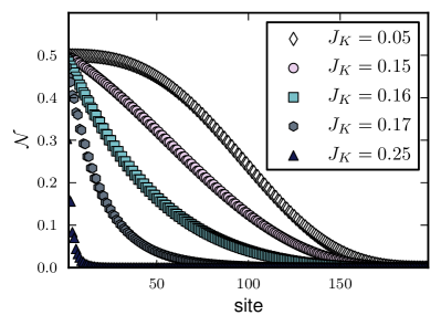
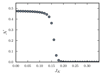
Figure 11: (a) Variational results for the negativity for different $J_{K}$ with $L=200$. (b) Variational results for the negativity for fixed size, $l=40$, of the subsystem x as a function of $J_{K}$ with $L=200$. All results are obtained at the MG-point with $\delta=0$.

As we saw in the previous section, the impurity entanglement for an even length system with $J_{K}=0$ can be seen as arising from an impurity valence bond (IVB). At the MG-point for $J_{K}=0$ this was calculated within the variational approach in reference [10]. Here we focus on the negativity $\mathcal{N}$ and the complete cross-over as $J_{K}$ is varied between $0$ and $1$. Variational results of $\mathcal{N}$ at different $J_{K}$ for a system of length $L=200$ (including the impurity site) are shown in figure 11(a). At $J_{K}=0$ the impurity entanglement is long-range, extending throughout the chain, but as $J_{K}$ is turned on it quickly becomes suppressed and for $J_{K}$ larger than $\sim 0.3$ it has all but disappeared reflecting the fact that the impurity valence bond now preferentially terminates close to the impurity site. For these non-zero values of $J_{K}$ the appropriate $\varphi_{sol}$ to use would then no longer be the wave-function of a free particle, as in equation (51), but instead a wave-function describing a localized state bound to the impurity site. The presence of such a localized state should be reflected in an exponentially decaying impurity entanglement away from the impurity site. For $J_{K}>0.15$ we have verified that the negativity $\mathcal{N}$ shown in figure 11(a) indeed has a tail decaying exponentially with the site index. The length scale, $\xi_{\mathrm{loc}}$, associated with this exponential decay is therefore clearly distinct from the bulk spin-spin correlation length in the system which here is effectively zero. The sharpness of the cross-over is illustrated in figure 11(b) where for a chain of $200$ spins the negativity with the region x containing $40$ spins is plotted versus $J_{K}$. As can be seen, $\mathcal{N}$ transitions from $\sim 0.5$ to $0$ very close to $J_{K}=0.15$. For $J_{K}\leq 0.15$ we have not been able to identify any exponentially decaying part in $\mathcal{N}$ as obtained within the variational approach even for systems substantially longer than $200$ and it appears that a finite $J_{K}^{c}\sim 0.15$ is needed to induce an exponential decay in $\mathcal{N}$. This would imply that the presence of a non-zero $J_{K}$ cannot be modelled as a simple one-dimensional potential well, since this would always have a bound-state independent of the depth of the potential well. Likely, an enlarged variational space for the calculation will change the value for $J_{K}^{c}$ and could possibly drive it all the way to zero. However, Bayat et al [11], using DMRG, do not find an exponential decay for $J_{2}=0.46$ and $J_{K}=0.16$ consistent with a non-zero $J_{K}^{c}$. Due to the complexity of the calculation of $\mathcal{N}$ in larger sub-spaces we have, however, been unable to complete such calculations.

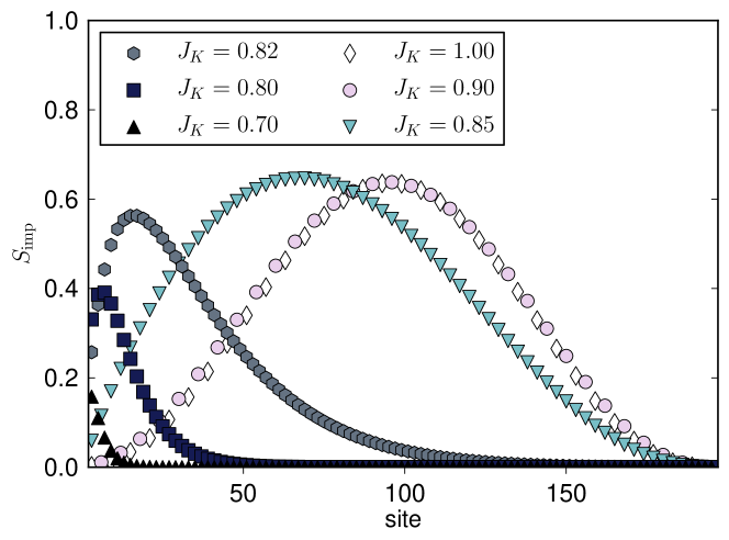
Figure 12: Variational results for the $S_{\mathrm{imp}}$ for different $J_{K}$ with $L=199$. All results are obtained at the MG-point with $\delta=0$. For clarity only a fraction of all data points is shown.

In a similar manner we can study the single particle entanglement (SPE) for general $J_{K}$ within the variational approach. Our results are shown in figure 12. The single particle entanglement arises from the presence of a single unpaired spin for odd $L$ which is always present in the ground-state for odd $L$. The unpaired spin moves freely throughout the system when $J_{K}=1$ but as $J_{K}$ is decreased away from 1 towards zero it rapidly becomes localized on the impurity site thereby quenching the impurity entanglement. As can be seen in figure 12 the impurity entanglement rapidly transitions around $J_{K}\sim 0.8-0.85$. While the variational approach agrees closely with DMRG data away from this transition region, some quantitative differences appear in this region due to the limitation of the Hilbert space used in the variational approach. The variational and DMRG results are however qualitatively the same and we have for clarity not included DMRG results in figure 12. We have verified that for $J_{K}\leq 0.85$ the data for $S_{\mathrm{imp}}$ shown in figure 12 develop an exponentially decaying part with an associated length scale, $\xi_{\mathrm{loc}}$, different from the bulk spin-spin correlation length. Also here, it appears that $\xi_{\mathrm{loc}}$ diverges before $J_{K}$ reaches 1 but this effect could possibly be due to finite-size effects in the DMRG calculations or limitations in the sub-space used in the variational calculations.

9 Impurity Entanglement with $\delta\neq 0$

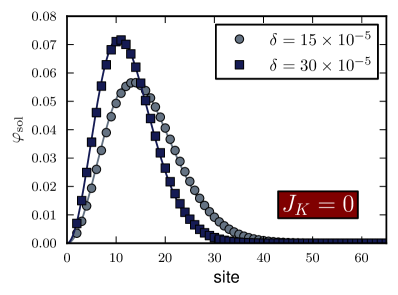
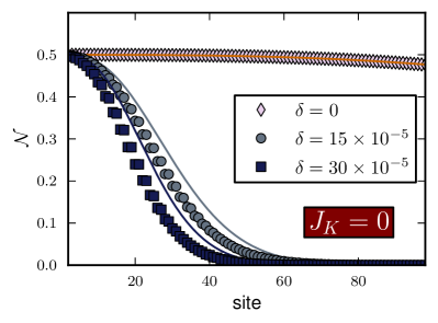
Figure 13: (a) Variational results for $\varphi_{\mathrm{sol}}$ (markers) compared to $\mathrm{Ai}(i/\xi+z)$ (lines) (see main text). (b) Variational results for the negativity at impurity-coupling $J_{K}=0$ for three values of the dimerization $\delta$ plotted along with the scaled IVB entanglement (lines). The calculations were done for a chain of length $L=500$, with $J_{2}=J/2$.

The variational approach that we employ here is straight forward to use for any $J_{2},\delta$ and $J_{K}$ and we now discuss our results for the impurity entanglement for non-zero explicit dimerization $\delta\neq 0$. As we stressed in the introduction the impurity entanglement can be long-range in these systems due to the near degeneracy of the two singlet ground-states of the chain with periodic boundary conditions. With a non-zero $\delta$ this degeneracy is lifted and we expect the impurity entanglement to decrease dramatically. Essentially, this is because when $\delta$ is increased it is more costly for the impurity to be entangled with far away parts of the systems: If the impurity is in a singlet with a spin far away, there are more dimers on weak bonds than if the impurity bonds with a site that is close to it. If we consider $L$ even, then, in order to have sizeable entanglement, the bulk of the chain must have a site in a valence-bond with the impurity-spin and this spin is then bound to one end of the chain [42].

For a chain with an even number of spins we expect to be able to describe $\mathcal{N}$ in terms of an IVB picture for which an estimate of $\varphi_{\mathrm{sol}}$ is needed for non-zero $\delta$. Such an estimate has been derived by Uhrig et al(reference [46]). They showed that to good approximation $\varphi_{\mathrm{sol}}(i)\propto\mathrm{Ai}(i/\xi+z)$, where $\mathrm{Ai(x)}$ is the Airy-function and $z_{1}=-2.3381$ is its biggest root. Here, the size of the area the impurity-spin binds to is roughly given by $\xi=(3m\delta/2)^{-1/3}$, where $m\approx 1/(1+7/\sqrt{65})$. Our variational approach directly yields the lowest state vector which is simply $\varphi_{\mathrm{sol}}$. In figure 13(a) we compare this directly to the $\mathrm{Ai}(i/\xi+z)$ where it can be seen that the agreement is good. It is noteworthy that the maximum in $\varphi_{\mathrm{sol}}$ is quite distant from the end of the chain in agreement with previous results.

We can use this result to estimate $\mathcal{N}$ using equation (50). In figure 13(b) we see typical graphs of the behaviour of the negativity as $\delta$ is increased with $J_{K}=0$ and $L=500$. The range over which the impurity-site is entangled is decreased upon increasing the dimerization. Figure 13(b) also includes the impurity valence bond entropy (IVB) obtained from equation (50) using the Airy functions for $\varphi_{\mathrm{sol}}$. For easier comparison with the negativity we scaled by a factor of $1/2\,\ln 2$. For $\delta=0$ we used equation (51) for $\varphi_{\mathrm{sol}}$. A reasonable agreement between $\mathcal{N}$ and the IVB contribution (solid lines) is observed. Overall, as one would expect, the impurity entanglement is now dramatically suppressed. Even for $\delta=15\times 10^{-5}$ the impurity entanglement is effectively zero beyond 60 sites. Following the above discussion we expect the extent over which the impurity entanglement is non-zero to diverge as $\delta^{-1/3}$ as dictated by $\xi$.

10 Conclusion

We have presented detailed discussion of how variational calculations can be used to calculate the negativity. This approach is quite generally applicable and should be very precise close to the MG-point. A complete characterization of the impurity entanglement for any $J_{K}$ can then be obtained. For $J_{K}=0$ ($L$ even) the impurity entanglement is long-range and extends throughout the system while for larger $J_{K}>0.15$ it decays exponentially with a length scale clearly different from the correlation length in the system. For $L$ odd the SPE present at $J_{K}=1$ is rapidly destroyed once $J_{K}$ is decreased below $J_{K}=0.8-0.85$. In both cases it would be valuable to perform higher precision calculations in order to determine whether or not a critical $J_{K}$ or $(1-J_{K})$ is needed to destroy the impurity entanglement. When a non-zero dimerization is introduced and the ground-state degeneracy is lifted, the impurity entanglement rapidly disappears. It would be interesting to investigate impurity entanglement in other gapped systems with degenerate singlet ground-states.

References

References

- [1] Calabrese P and Cardy J. Entanglement entropy and quantum field theory. J. Stat. Mech., P06002, 2004.
- [2] White S R. Density matrix formulation for quantum renormalization groups. Phys. Rev. Lett., 69:2863, 1992.
- [3] Zhou H-Q, Barthel T, Fjaerestad J, and Schollwöck U. Entanglement and boundary critical phenomena. Phys. Rev. A, 84:050305(R), 2006.
- [4] Laflorencie N, Sørensen E S, Chang M-S, and Affleck I. Boundary effects in the critical scaling of entanglement entropy in 1D systems. Phys. Rev. Lett., 96:100603–4, 2006.
- [5] Cho S Y and McKenzie R H. Quantum entanglement in the two-impurity Kondo model. Phys. Rev. A, 73:012109, 2006.
- [6] Kopp A and Le Hur K. Universal and measurable entanglement entropy in the spin-boson model. Phys. Rev. Lett., 98:220401, 2007.
- [7] Le Hur K, Doucet-Beaupre P, and Hofstetter W. Entanglement and criticality in quantum impurity systems. Phys. Rev. Lett., 99:126801, 2007.
- [8] Le Hur K. Entanglement entropy, decoherence, and quantum phase transitions of a dissipative two-level system. Annals of Physics, 323:2208–2240, 2007.
- [9] Sørensen E S, Chang M-S, Laflorencie N, and Affleck I. Impurity entanglement entropy and the Kondo screening cloud. J. Stat. Mech., L01001, 2007.
- [10] Sørensen E S, Chang M-S, Laflorencie N, and Affleck I. Quantum impurity entanglement. J. Stat. Mech., 2007:P08003, 2007.
- [11] Bayat A, Sodano P, and Bose S. Negativity as the entanglement measure to probe the Kondo regime in the spin-chain Kondo model. Phys. Rev. B, 81:064429, 2010.
- [12] Sodano P, Bayat A, and Bose S. Kondo cloud mediated long-range entanglement after local quench in a spin chain. Phys. Rev. B, 81:100412, 2010.
- [13] Eriksson E and Johannesson H. Impurity entanglement entropy in Kondo systems from conformal field theory. Arxiv preprint arXiv:1102.2492, 2011.
- [14] Affleck I, Laflorencie N, and Sørensen E S. Entanglement entropy in quantum impurity systems and systems with boundaries. Journal of Physics A: Mathematical and Theoretical, 42:504009, 2009.
- [15] Bose S. Quantum communication through an unmodulated spin chain. Phys. Rev. Lett., 91:207901, 2003.
- [16] Christandl M, Datta N, Ekert A, and Landahl A J. Perfect state transfer in quantum spin networks. Phys. Rev. Lett., 92:187902, 2004.
- [17] Christandl M, Datta N, Dorlas T C, Ekert A, Kay A, and Landahl A J. Perfect transfer of arbitrary states in quantum spin networks. Phys. Rev. A (Atomic, Molecular, and Optical Physics), 71:032312, 2005.
- [18] Burgarth D and Bose S. Perfect quantum state transfer with randomly coupled quantum chains. New J. Phys., 7:135, 2005.
- [19] Burgarth D, Giovannetti V, and Bose S. Efficient and perfect state transfer in quantum chains. J. Phys. A, 38:6793, 2005.
- [20] Wójcik A, Luczak T, Kurzyński P, Grudka A, Gdala T, and Bednarska M. Unmodulated spin chains as universal quantum wires. Phys. Rev. A, 72:034303, 2005.
- [21] Plenio M B and Semião F L. High efficiency transfer of quantum information and multiparticle entanglement generation in translation-invariant quantum chains. New J. Phys., 7:73, 2005.
- [22] Campos Venuti L, Degli Esposti Boschi C, and Roncaglia M. Long-distance entanglement in spin systems. Phys. Rev. Lett., 96:247206, 2006.
- [23] Campos Venuti L, Degli Esposti Boschi C, and Roncaglia M. Qubit teleportation and transfer across antiferromagnetic spin chains. Phys. Rev. Lett., 99:060401, 2007.
- [24] von Neumann J. Gött. Nachr., 273, 1927.
- [25] Wehrl A. General properties of entropy. Rev. Mod. Phys., 50:221, 1978.
- [26] Vidal G and Werner R F. Computable measure of entanglement. Phys. Rev. A, 65:032314, 2002.
- [27] Affleck I, Kennedy T, Lieb E H, and Tasaki H. Rigorous results on valence-bond ground states in antiferromagnets. Phys. Rev. Lett., 59:799–802, 1987.
- [28] Affleck I, Kennedy T, Lieb E H, and Tasaki H. Valence bond ground states in isotropic quantum antiferromagnets. Commun. Math. Phys., 115:477–528, 1988.
- [29] Tribedi A and Bose I. Quantum critical point and entanglement in a matrix-product ground state. Phys. Rev. A, 75:042304, 2007.
- [30] Tribedi A and Bose I. Entanglement and fidelity signatures of quantum phase transitions in spin liquid models. Phys. Rev. A, 77:032307, 2008.
- [31] Hirano T and Hatsugai Y. Entanglement entropy of one-dimensional gapped spin chains. J. Phys. Soc. Japan, 76:074603, 2007.
- [32] Fáth G, Legeva Ö, Lájko P, and Iglói F. Logarithmic delocalization of end spins in the antiferromagnetic Heisenberg chain. Phys. Rev. B, 73:214447, 2006.
- [33] Fan H, Korepin V, and Roychowdhury V. Entanglement in a valence-bond solid state. Phys. Rev. Lett., 93:227203, 2004.
- [34] Alipour S, Karimipour V, and Mermarzadeh L. Entanglement and quantum phase transitions in matrix-product spin-1 chains. Phys. Rev. A, 75:052322, 2007.
- [35] Geraedts S D and Sørensen E S. Exact results for the bipartite entanglement entropy of the AKLT spin-1 chain. Journal of Physics A: Mathematical and Theoretical, 43:185304, 2010.
- [36] Majumdar C K. Antiferromagnetic model with known ground state. Journal of Physics C: Solid State Physics, 3:911–915, 1970.
- [37] Haldane F D M. Spontaneous dimerization in the Heisenberg antiferromagnetic chain with competing interactions. Phys. Rev. B, 25:4925, 1982.
- [38] Eggert S. Numerical evidence for multiplicative logarithmic corrections from marginal operators. Phys. Rev. B, 54:9612, 1996.
- [39] Eggert S and Affleck I. Magnetic impurities in half-integer-spin Heisenberg antiferromagnetic chains. Phys. Rev. B, 46:10866, 1992.
- [40] Laflorencie N, Sørensen E S, and Affleck I. The kondo effect in spin chains. J. Stat. Mech., P02007, 2008.
- [41] Shastry B S and Sutherland B. Excitation spectrum of a dimerized Next-Neighbor antiferromagnetic chain. Phys. Rev. Lett., 47:964, 1981.
- [42] Sørensen E S, Affleck I, Augier D, and Poilblanc D. Soliton approach to spin-Peierls antiferromagnets: Large-scale numerical results. Phys. Rev. B, 58:R14701, 1998.
- [43] Caspers W J and Magnus W. Some exact excited states in a linear antiferromagnetic spin system. Phys. Lett. A, 88A:103, 1982.
- [44] Caspers W J, Emmett K M, and Magnus W. The Majumdar-Ghosh chain. Twofold ground state and elementary excitations. J. Phys. A, 17:2687, 1984.
- [45] Beach K S D and Sandvik A W. Some formal results for the valence bond basis. Nuclear Physics B, 750:142–178, 2006.
- [46] Uhrig G S, Schönfeld F, Laukamp M, and Dagotto E. Unified quantum mechanical picture for confined spinons in dimerized and frustrated spin chains. The European Physical Journal B, 7:67, 1999.
- [47] Sutherland B. Systems with resonating-valence-bond ground states: Correlations and excitations. Phys. Rev. B, 37:3786, 1988.