Stellar mass-to-light ratio gradients in galaxies: correlations with mass.

Abstract

We analyze the stellar mass-to-light ratio ($M/L$) gradients in a large sample of local galaxies taken from the Sloan Digital Sky Survey, spanning a wide range of stellar masses and morphological types. As suggested by the well known relationship between mass-to-light ($M/L$) ratios and colors, we show that $M/L$ gradients are strongly correlated with colour gradients, which we trace to the effects of age variations. Stellar $M/L$ gradients generally follow patterns of variation with stellar mass and galaxy type that were previous found for colour and metallicty gradients. In late-type galaxies $M/L$ gradients are negative, steepening with increasing mass. In early-type galaxies $M/L$ gradients are shallower while presenting a two-fold trend: they decrease with mass up to a characteristic mass of $\mbox{$M_{*}$}\sim 10^{10.3}\mbox{$M_{\odot}$}$ and increase at larger masses. We compare our findings with other analyses and discuss some implications for galaxy formation and for dark matter estimates.

1 Introduction

Colour and absorption line gradients are markers of stellar population variations within galaxies, providing important clues to galaxy evolution (e.g. Spolaor et al. 2009; Gonzalez-Perez et al. 2011; Rawle et al. 2010; Spolaor et al. 2010; Tortora et al. 2010a, herafter T+10, Tortora et al. 2011). Although spectral features are less ambiguous probes of stellar population properties than colours are (e.g. Spolaor et al. 2009, 2010; 2010; Rawle et al. 2010), there are only small samples available outside the nuclear regions of galaxies. Fortunately, studies based on colours turn out to provide, on average, similar age and metallicity estimates to spectral studies (e.g. T+10), allowing for much larger surveys of radially-extended stellar populations.

In T+10 we analyzed colour gradients within an effective radius ($R_{\rm eff}$) for an extensive sample of low-redshift galaxies based on SDSS data (Blanton et al. 2005), including both early-type (ETGs) and late-type (LTGs) galaxies. We carried out simple stellar populations analyses, fitting synthetic models to the observed colours to derive estimated age and metallicity gradients, and stellar masses (see T+10 and later in the paper for further details). The main results found can be summarized as follows:

1. Colour gradients are, on average, negative (i.e. galaxies are redder in the centre), except for galaxies with lower stellar masses ($\mbox{$M_{*}$}\mathrel{\hbox to0.0pt{\lower 3.5pt\hbox{\hskip 0.5pt$\sim$}\hss}\raise 0.5pt\hbox{$<$}}10^{9.3}\,\rm\mbox{$M_{\odot}$}$) which tend to have null or positive gradients. At fixed mass, LTGs have steeper gradients than ETGs, whose colour profiles in general show milder variations .

2. The colour gradients of LTGs decrease systematically with mass while the trend for ETGs changes near a mass of $\mbox{$M_{*}$}\sim 10^{10.3}\,\rm\mbox{$M_{\odot}$}$: systematically decreasing and increasing at lower and higher masses, respectively.

3. The primary driver of the colour gradients, mainly for galaxies with older centers, is metallicity variations, with age gradients playing a secondary role. For LTGs, the metallicity gradients tend to be steeper for higher masses, The same is true for ETGs except that for masses above $\mbox{$M_{*}$}\sim 10^{10.3}\,\rm\mbox{$M_{\odot}$}$, the (negative) gradients are fairly invariant or slightly increasing with mass.

4. At fixed mass, galaxies with older centres have the shallowest metallicity and age gradients.

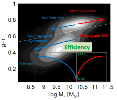
Figure 1: Diagram of colour versus stellar mass for the local SDSS galaxy sample analyzed in T+10. The grey-scale contours show the density of data points, with brighter regions marking higher densities. The thin white line separates the red sequence and blue cloud. The arrows and the curves in the inset panel give information about the efficiency of the phenomena which drive the two fold trend we discuss in the paper (see T+10 for further details). AGN feedback and merging are important at high mass with an efficiency that increases with mass, while SN feedback and gas inflow drive the galaxy evolution at lower masses, with an efficiency that is larger at the lowest masses.

We found that these results were generally consistent with others in the literature (e.g. Spolaor et al. 2009; Rawle et al. 2010) once different galaxy selection effects were taken into account.

The overall observational picture can be framed within the predictions of hydrodynamical and chemodynamical simulations of galaxy formation (Bekki & Shioya 1999; Kawata 2001; Kawata & Gibson 2003; 2004; Hopkins et al. 2009; Pipino et al. 2010; Tortora et al. 2011) which include various physical processes that can influence the gradients: supernovae and AGN feedback, galaxy mergers, interactions with environment, etc. A fresh and qualitative overview of this physical scenario is given by Fig. 1, where we show the isodensity contours for the colour-mass diagram (which we have already discussed in T+10) and superimpose some lines (in the inset) and arrows which indicate the efficiency of the highlighted physical processes. In particular, the observations for high-mass ETGs seem to generally suggest the influence of mergers and AGN feedback (2004; Hopkins et al. 2009; Sijacki et al. 2007), with an efficiency possibly increasing with mass (see red arrows and lines in the inset panel). On the other hand, the population gradients of LTGs and less massive ETGs may be mainly driven by infall and supernovae feedback (Larson 1974, 1975; Kawata 2001; Kawata & Gibson 2003; 2004; Pipino et al. 2010; Tortora et al. 2011), which are more efficient at very low masses (see blue lines and arrows).

In this paper we consider the implications of the observed colour, metallicity and age gradients from T+10 for variations of stellar mass-to-light ratio $M/L$ with radius. This issue is relevant for understanding the detailed distribution of mass within galaxies: both the stellar mass and the dark matter, whose distribution is inferred by substracting the stellar mass from the total dynamical mass. There has been scarcely any literature to date that focussed on this topic, except for a study in spiral galaxies by Portinari & Salucci (2010).

As a first approximation, one could use single-colour semi-empirical models such as those of Bell & de Jong (2001) and Bell et al. (2003, B03 hereafter) to go directly from colour gradients to $M/L$ gradients. However, we wish to make use of multiple colours, to allow for departures of individual galaxies from mean trends, to explore the systematics thoroughly, and to trace the dependence on stellar parameters, like age and metallicity.

This paper is organized as follows. The sample and the spectral analysis are discussed in §2, in where we also show the ability of our fitting procedure to recover the correct $M/L$ gradients, and we examine possible systematics. The results are shown in §3, while §4 is devoted to a discussion of the physical implications and conclusions.

2 Data and spectral analysis

Our database consists of $50\,000$ low redshift ($0.0033\leq z\leq 0.05$) galaxies in the NYU Value-Added Galaxy Catalog extracted from SDSS DR4 (Blanton et al. 2005, hereafter B05), recently analyzed in T+10. Following T+10, we have identified ETGs as those systems with a r-band S$\rm\acute{e}$rsic index satisfying the condition $2.5\leq n\leq 5.5$ and with a concentration index $C>2.6$. The final ETG sample consists of $10\,508$ galaxies. Of the remaining entries of our database, $\sim 27\,800$ are LTGs, defined as objects with $C\leq 2.6$, $n\leq 2.5$, and $\mbox{$\sigma_{0}$}\leq 150~{}\rm km/s$.

Table 1: Recovery of stellar population parameters from Monte Carlo simulations. A purely random sample of galaxies is generated, leaving the ages and metallicities free to vary across the whole range. We list the median error and the 25-75 percent scatter in the gradient $\Delta(X)=X_{\rm fit}-X_{\rm in}$, where $X_{\rm in}$ and $X_{\rm fit}$ are the input and fitted gradients with $X=\mbox{$\nabla_{\rm\tiny\mbox{$\Upsilon_{*}$}}$}$, $\nabla_{\rm age}$ and $\nabla_{\rm Z}$. The data are divided in three subsamples, on the basis of the input $M/L$s at $R_{2}$. Different initial perturbations $\delta$ and the results (1) with optical only ($ugriz$) (2) optical and near-IR ($ugrizJHKs$), and (3) optical and UV ($ugrizFUVNUV$) are shown.

	$\log\mbox{$\Upsilon_{*}$}_{in,2}\leq 0$			$0<\log\mbox{$\Upsilon_{*}$}_{in,2}\leq 0.4$			$\log\mbox{$\Upsilon_{*}$}_{in,2}>0.4$
	$ugriz$	$ugrizJHKs$	$ugrizFUVNUV$	$ugriz$	$ugrizJHKs$	$ugrizFUVNUV$	$ugriz$	$ugrizJHKs$	$ugrizFUVNUV$
	$\nabla_{\rm\tiny\mbox{$\Upsilon_{*}$}}$
$\delta=0.01$	$0_{-0.02}^{+0.02}$	$0_{-0.02}^{+0.02}$	$0_{-0.02}^{+0.02}$	$0_{-0.03}^{+0.04}$	$0_{-0.02}^{+0.02}$	$0_{-0.02}^{+0.02}$	$0_{-0.04}^{+0.03}$	$0_{-0.03}^{+0.02}$	$0_{-0.02}^{+0.02}$
$\delta=0.03$	$0_{-0.05}^{+0.04}$	$0_{-0.03}^{+0.03}$	$0_{-0.02}^{+0.02}$	$0.01_{-0.06}^{+0.10}$	$0_{-0.03}^{+0.03}$	$0_{-0.03}^{+0.03}$	$-0.01_{-0.07}^{+0.07}$	$0_{-0.04}^{+0.04}$	$0_{-0.02}^{+0.02}$
$\delta=0.05$	$0_{-0.07}^{+0.06}$	$0_{-0.04}^{+0.04}$	$0_{-0.03}^{+0.02}$	$0.02_{-0.10}^{+0.12}$	$0.01_{-0.05}^{+0.05}$	$0_{-0.04}^{+0.04}$	$-0.01_{-0.10}^{+0.09}$	$0_{-0.06}^{+0.06}$	$0_{-0.03}^{+0.03}$
	$\nabla_{\rm age}$
$\delta=0.01$	$0_{-0.04}^{+0.04}$	$0_{-0.02}^{+0.03}$	$0_{-0.02}^{+0.02}$	$0.01_{-0.05}^{+0.06}$	$0_{-0.03}^{+0.03}$	$0_{-0.03}^{+0.03}$	$0.01_{-0.06}^{+0.06}$	$0_{-0.04}^{+0.04}$	$0_{-0.03}^{+0.03}$
$\delta=0.03$	$0_{-0.08}^{+0.08}$	$0_{-0.04}^{+0.05}$	$0_{-0.03}^{+0.03}$	$0.02_{-0.12}^{+0.16}$	$0_{-0.05}^{+0.05}$	$0_{-0.04}^{+0.04}$	$-0.02_{-0.12}^{+0.11}$	$0_{-0.06}^{+0.07}$	$0_{-0.04}^{+0.03}$
$\delta=0.05$	$-0.01_{-0.12}^{+0.13}$	$0_{-0.07}^{+0.07}$	$0_{-0.04}^{+0.04}$	$0.04_{-0.17}^{+0.21}$	$0.01_{-0.08}^{+0.08}$	$0.01_{-0.06}^{+0.06}$	$-0.02_{-0.16}^{+0.15}$	$-0.01_{-0.09}^{+0.09}$	$0_{-0.05}^{+0.05}$
	$\nabla_{\rm Z}$
$\delta=0.01$	$0_{-0.05}^{+0.06}$	$0_{-0.03}^{+0.03}$	$0_{-0.03}^{+0.03}$	$-0.01_{-0.07}^{+0.06}$	$0_{-0.03}^{+0.03}$	$0_{-0.04}^{+0.03}$	$0.00_{-0.05}^{+0.05}$	$0_{-0.03}^{+0.03}$	$0_{-0.03}^{+0.03}$
$\delta=0.03$	$0_{-0.12}^{+0.12}$	$0_{-0.06}^{+0.05}$	$0_{-0.04}^{+0.04}$	$-0.02_{-0.18}^{+0.16}$	$0_{-0.05}^{+0.05}$	$0_{-0.04}^{+0.04}$	$0.02_{-0.10}^{+0.12}$	$0_{-0.05}^{+0.05}$	$0_{-0.04}^{+0.04}$
$\delta=0.05$	$0.01_{-0.20}^{+0.19}$	$0_{-0.08}^{+0.09}$	$0_{-0.05}^{+0.05}$	$-0.03_{-0.26}^{+0.22}$	$0.01_{-0.08}^{+0.09}$	$-0.01_{-0.06}^{+0.06}$	$0.02_{-0.15}^{+0.16}$	$-0.01_{-0.07}^{+0.07}$	$0_{-0.05}^{+0.05}$

Table 2: Median errors as in Table 1, but for $\delta=0.05$. Ages and metallicities are generated to have average $\nabla_{\rm age}$ and $\nabla_{\rm Z}$ around fixed values.

	$\log\mbox{$\Upsilon_{*}$}_{in,2}\leq 0$			$0<\log\mbox{$\Upsilon_{*}$}_{in,2}\leq 0.4$			$\log\mbox{$\Upsilon_{*}$}_{in,2}>0.4$
	$ugriz$	$ugrizJHKs$	$ugrizFUVNUV$	$ugriz$	$ugrizJHKs$	$ugrizFUVNUV$	$ugriz$	$ugrizJHKs$	$ugrizFUVNUV$
	$\nabla_{\rm\tiny\mbox{$\Upsilon_{*}$}}$
$\mbox{$\nabla_{\rm age}$}\sim 0.09$, $\mbox{$\nabla_{\rm Z}$}\sim-0.32$	$-0.01_{-0.09}^{+0.10}$	$0.01_{-0.06}^{+0.07}$	$0_{-0.03}^{+0.03}$	$-0.01_{-0.12}^{+0.12}$	$0_{-0.08}^{+0.07}$	$0_{-0.05}^{+0.04}$	$-0.06_{-0.14}^{+0.11}$	$-0.01_{-0.08}^{+0.06}$	$-0.01_{-0.04}^{+0.03}$
$\mbox{$\nabla_{\rm age}$}\sim-0.12$, $\mbox{$\nabla_{\rm Z}$}\sim-0.47$	$-0.02_{-0.10}^{+0.07}$	$0_{-0.06}^{+0.05}$	$0_{-0.03}^{+0.03}$	$-0.03_{-0.12}^{+0.12}$	$0_{-0.07}^{+0.07}$	$-0.01_{-0.05}^{+0.04}$	$-0.07_{-0.14}^{+0.11}$	$-0.02_{-0.07}^{+0.06}$	$-0.01_{-0.03}^{+0.03}$
$\mbox{$\nabla_{\rm age}$}\sim 0.35$, $\mbox{$\nabla_{\rm Z}$}\sim-0.08$	-	-	-	-	-	-	$-0.05_{-0.12}^{+0.09}$	$-0.01_{-0.07}^{+0.06}$	$0_{-0.03}^{+0.03}$
	$\nabla_{\rm age}$
$\mbox{$\nabla_{\rm age}$}\sim 0.09$, $\mbox{$\nabla_{\rm Z}$}\sim-0.32$	$-0.05_{-0.16}^{+0.20}$	$0_{-0.10}^{+0.10}$	$0_{-0.06}^{+0.05}$	$-0.02_{-0.21}^{+0.21}$	$0.01_{-0.11}^{+0.11}$	$-0.01_{-0.08}^{+0.07}$	$-0.10_{-0.25}^{+0.19}$	$-0.02_{-0.12}^{+0.10}$	$-0.01_{-0.06}^{+0.04}$
$\mbox{$\nabla_{\rm age}$}\sim-0.12$, $\mbox{$\nabla_{\rm Z}$}\sim-0.47$	$-0.03_{-0.16}^{+0.13}$	$0_{-0.08}^{+0.08}$	$-0.01_{-0.05}^{+0.05}$	$-0.05_{-0.20}^{+0.19}$	$0_{-0.10}^{+0.11}$	$-0.01_{-0.07}^{+0.06}$	$-0.13_{-0.24}^{+0.18}$	$-0.03_{-0.10}^{+0.10}$	$-0.01_{-0.06}^{+0.05}$
$\mbox{$\nabla_{\rm age}$}\sim 0.35$, $\mbox{$\nabla_{\rm Z}$}\sim-0.08$	-	-	-	-	-	-	$-0.08_{-0.21}^{+0.16}$	$-0.02_{-0.11}^{+0.10}$	$-0.01_{-0.05}^{+0.05}$
	$\nabla_{\rm Z}$
$\mbox{$\nabla_{\rm age}$}\sim 0.09$, $\mbox{$\nabla_{\rm Z}$}\sim-0.32$	$0.11_{-0.23}^{+0.17}$	$0.01_{-0.09}^{+0.08}$	$0.01_{-0.07}^{+0.08}$	$0.03_{-0.21}^{+0.24}$	$0_{-0.09}^{+0.09}$	$0.01_{-0.06}^{+0.07}$	$0.09_{-0.18}^{+0.23}$	$0.02_{-0.09}^{+0.08}$	$0.02_{-0.06}^{+0.06}$
$\mbox{$\nabla_{\rm age}$}\sim-0.12$, $\mbox{$\nabla_{\rm Z}$}\sim-0.47$	$0.05_{-0.18}^{+0.19}$	$0_{-0.10}^{+0.11}$	$0.01_{-0.05}^{+0.06}$	$0.05_{-0.18}^{+0.23}$	$0_{-0.08}^{+0.08}$	$-0.01_{-0.06}^{+0.07}$	$0.10_{-0.15}^{+0.22}$	$0.02_{-0.07}^{+0.08}$	$0.02_{-0.05}^{+0.06}$
$\mbox{$\nabla_{\rm age}$}\sim 0.35$, $\mbox{$\nabla_{\rm Z}$}\sim-0.08$	-	-	-	-	-	-	$0.06_{-0.14}^{+0.19}$	$0.02_{-0.07}^{+0.08}$	$0_{-0.05}^{+0.05}$

We have used the multi-band structural parameters given by B05 to derive the colour profile $(X-Y)(R)$ of each galaxy as the differences between the (logarithmic) surface brightness measurements in the two bands, $X$ and $Y$. We have defined the colour gradient as the angular coefficient of the relation $X-Y$ vs $\log R/\mbox{$R_{\rm eff}$}$, $\displaystyle\nabla_{X-Y}=\frac{\delta(X-Y)}{\delta\log(R/R_{\rm eff})}$, measured in mag dex^-1 (omitted in the following), where $R_{\rm eff}$ is the r-band effective radius. By definition, a positive gradient, $\nabla_{X-Y}>0$, means that a galaxy is redder as $R$ increases, while it is bluer outward for a negative gradient. The fit of synthetic colours is performed on the colours at $R_{1}=\mbox{$R_{\rm eff}$}/10$ and $R_{2}=\mbox{$R_{\rm eff}$}$ and on the total integrated colours.

The stellar population properties (age, metallicity and $M/L$) are derived by fitting Bruzual & Charlot (2003, hereafter BC03) “single burst” synthetic stellar models to the observed colours. Age and metallicity are free to vary, and a Chabrier (2001) initial mass function (IMF) is assumed. Stellar parameter gradients are defined as $\displaystyle\nabla_{W}=\frac{\delta(W)}{\delta\log(R/R_{\rm eff})}$, where $W=(age,Z,\mbox{$\Upsilon_{*}$})$ are the estimated age, metallicity and $M/L$. Because of the definitions adopted for $R_{1}$ and $R_{2}$, an easier and equivalent definition can be used, in fact, we define $\mbox{$\nabla_{\rm age}$}=\log[\rm age_{2}/\rm age_{1}]$, $\mbox{$\nabla_{\rm Z}$}=\log[Z_{2}/Z_{1}]$ and $\mbox{$\nabla_{\rm\tiny\mbox{$\Upsilon_{*}$}}$}=\log[\rm\mbox{$\Upsilon_{*}$}_{2}/\rm\mbox{$\Upsilon_{*}$}_{1}]$ where (age_i, $Z_{i}$, $\mbox{$\Upsilon_{*}$}_{i}$), with $i=1,2$, are the estimated parameters at $R_{1}$ and $R_{2}$, respectively. In the present paper we will concentrate on the analysis of the $M/L$ gradients, $\nabla_{\rm\tiny\mbox{$\Upsilon_{*}$}}$, in terms of stellar mass and velocity dispersion. The dataset, including main stellar parameters and gradients, is available at: http://www.itp.uzh.ch/$\rm\sim$ctortora/gradient_data.html.

Before proceeding, we check for systematic effects on our $\nabla_{\rm\tiny\mbox{$\Upsilon_{*}$}}$ estimates from the stellar population fits. Because of the well known age-metallicity degeneracy (Worthey 1994, Bruzual & Charlot 2003, Gallazzi et al. 2005), the stellar population parameters and the gradients might be biased when using the optical colours only, as we do now. Widening the wavelength baseline to include near-infrared (NIR) colours should ameliorate the degeneracy. In T+10 we checked age and metallicity inferences using optical versus optical+NIR constraints, and found little systematic difference. Here we will carry out a similar analysis of the $M/L$ gradients, using a suite of Monte Carlo simulations.

We extract some sets of simulated galaxy spectra from our BC03 spectral energy distribution libraries with random, uncorrelated stellar parameters and gradients. We start from generating data with fully random ages and metallicities, and then we also analyze the cases when the stellar parameters are constrained within fixed intervals, generating not-zero sample average gradients. We extract the input galaxy colours and add simulated measurement errors, as randomly extracted steps from the interval ($-\delta$,$+\delta$), with $\delta=0.01,0.03,0.05$. We apply our fitting procedure, searching for the best model in our synthetic library, which reproduces the colours of each of the simulated galaxies and then compare the output parameter estimates to the input model values. We perform the fit (1) using only the optical SDSS bands $ugriz$ and (2) adding NIR photometry ($J$, $H$ and $Ks$; Jarrett et al. 2003) and (3) ultraviolet photometry (NUV and FUV; Martin et al. 2005). We define the median error in the gradients as $\Delta(X)=X_{\rm fit}-X_{\rm in}$, where $X_{\rm in}$ and $X_{\rm fit}$ are the input and fitted gradients with $X=\mbox{$\nabla_{\rm\tiny\mbox{$\Upsilon_{*}$}}$}$, $\nabla_{\rm age}$ and $\nabla_{\rm Z}$, which we show in Tables 1 and 2.

Starting from the purely random case shown in Table 1, we have found that, adding the NIR or UV data, both the $M/L$ values and their gradients are perfectly recovered with a very little scatter. With optical data only, the uncertainties are doubled (around 0.1 in $\Delta(\mbox{$\nabla_{\rm\tiny\mbox{$\Upsilon_{*}$}}$})$) and there is a small systematic shift in the gradients (of $\log\mbox{$\nabla_{\rm\tiny\mbox{$\Upsilon_{*}$}}$}\sim 0.01-0.02$ for the worst case analyzed), but the results are fairly well recovered with no spurious trends expected. We notice that the median results are quite independent of the range adopted for the input $\mbox{$\Upsilon_{*}$}_{2}$, and only slight differences in the scatter are found. Although we will be mainly interested in the trends of $\nabla_{\rm\tiny\mbox{$\Upsilon_{*}$}}$ with mass and velocity dispersion, we have also checked the systematics in age and metallicity gradients. We find similar results to the case of $\nabla_{\rm\tiny\mbox{$\Upsilon_{*}$}}$ discussed above, but slightly larger shifts in the median and larger scatters ($\sim 0.2$ in the worst cases) when only the optical is used. In Table 2, calculating the sample averages, we start with the input values $\mbox{$\nabla_{\rm age}$}\neq 0$ and $\mbox{$\nabla_{\rm Z}$}\neq 0$. Here the median errors and the scatters increase, but the conclusions discussed above are qualitatively confirmed. When optical data are used, for high $\mbox{$\Upsilon_{*}$}_{2}$ we have the worst discrepancies in the estimated $M/L$ gradients amounting to $\sim-0.05$, $-0.07$. For age and metallicity gradients, we could underestimate (overestimate) the age (metallicity) gradients of $\sim 0.1$, which is reduced to $\sim 0.02$ when near-IR or UV are included.

Thus, in many cases we have found that the median errors are acceptable and within the typical sample scatter and the uncertainties due to the adopted stellar population prescription. We will consider these results as qualitative indications of the effects on estimated gradients caused by systematics.

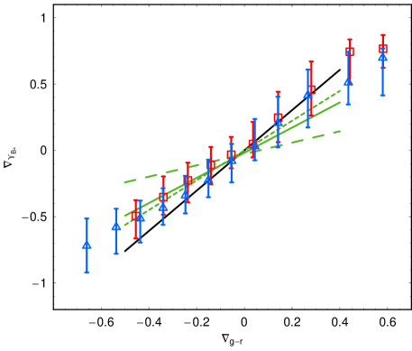
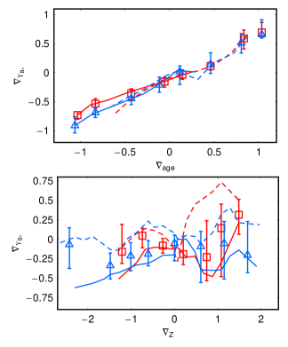
Figure 2: Left. $M/L$ gradient as a function of $g-r$ gradient for ETGs (red squares) and LTGs (blue triangles). Medians of the gradients (in bins of colour gradient) are plotted together with the 25-75 per cent quantiles, shown as error bars. The lines are for the gradients obtained using the best fitted $M/L$-colour relations in B03. The relationships between the $g$-band $M/L$ ($g$-band is approximatively the same as the $B$-band) and $g-r$ (solid black line), $u-g$ (long dashed green line), $g-i$ (short dashed green line) and $g-z$ (green line) are adopted and the recovered $\nabla_{\rm\tiny\mbox{$\Upsilon_{*}$}}$ are plotted as a function of $\nabla_{\rm g-r}$. Right. Age (top) and metallicity (bottom) gradients as a function of $g-r$ colour gradient. Solid and dashed lines show systems whose centres are older and younger than 6 Gyr, respectively. $M/L$ and colour gradients are tightly correlated for both ETGs and LTGs, and, while $\nabla_{\rm\tiny\mbox{$\Upsilon_{*}$}}$ correlates with $\nabla_{\rm age}$, no clear trend is observed in terms of $\nabla_{\rm Z}$.

3 Results

In this section we discuss first the $M/L$ gradients in terms of colour, age and metallicity gradients and then as a function of stellar mass and velocity dispersion, paying attention to the role of central age in the observed correlations.

3.1 Dependence on colour, age and metallicity gradients

We start by plotting in Fig. 2 the $M/L$ gradients as a function of $g-r$ colour gradient ($\nabla_{\rm g-r}$) for ETGs and LTGs. The two quantities are strongly and positively correlated and no statistically significant difference between the morphological types is found. While such a correlation is not surprising owing to the well known-correlations between colours and $M/L$ (Bell & de Jong 2001; B03), which should apply to all radii thus producing the relationship between $\nabla_{\rm\tiny\mbox{$\Upsilon_{*}$}}$ and $\nabla_{\rm g-r}$, there are important details to consider. Bell & de Jong (2001) have adopted different evolution models for LTGs to establish some linear correlations between integrated total colours and the corresponding $M/L$ determining some best fit relations between these two quantities, which have been proven to work for ETGs as well (Bell et al. 2003). Adopting the solar metallicity models in Bell & de Jong (2001) we have found a good agreement with Bruzual & Charlot (2003) or Maraston (2005) synthetic prescriptions in ETGs with high $M/L$, while at low $M/L$ Bell & de Jong (2001) overestimates the $M/L$ (see Tortora et al. (2009) for further details). In the left panel of Fig. 2 we compare our $\nabla_{\rm\tiny\mbox{$\Upsilon_{*}$}}$-$\nabla_{\rm g-r}$ trends with the ones (solid and dashed lines) derived from the B03 best fitted relations, finding a good agreement. The black and green lines plotted in Fig. 2 are derived by the relations between the g-band $M/L$ and the colours ($u-g$, $g-r$, $g-i$ and $g-z$) from B03. We insert in these relations the measured colour for each galaxy in our sample, deriving the corresponding $M/L$. This operation is made for both the radii $R_{1}$ and $R_{2}$, thus we can calculate the $M/L$ gradients. Finally, the plotted lines are obtained, first calculating medians of $\nabla_{\rm\tiny\mbox{$\Upsilon_{*}$}}$ in bins of $\nabla_{\rm g-r}$ and then fitting a straight line. We see that the best fitted relations depend on the colours adopted in the colour–$M/L$ relations from B+03 to derive the $M/L$ gradients. For instance, we observe a flattening of the $\nabla_{\rm\tiny\mbox{$\Upsilon_{*}$}}$–$\nabla_{\rm g-r}$ relation when using colours probing redder wavelengths, i.e. $g-i$ and $g-z$, but a shallower trend is obtained when $u-g$ is adopted. The agreement is quite good for moderate colour gradients, while for very steep positive or negative gradients some departures are observed.

Despite the good agreement, the very simplified approach in Bell & de Jong (2001) and B03 has some strong limitations. In fact, a) the B03 relations hold for integrated quantities, thus the radial variation of the $M/L$ can be derived if one assumes that the same relations apply at different apertures and in general, the zero-point and the slope of these fitted linear relations would depend on the radius adopted and b) these relations do not take into account the stellar parameters (e.g. age and metallicity at each radius) thus they do not allow to catch the full physics behind these correlations. These shortcomings are overcome by our multi-colour direct stellar population analysis which connects the $M/L$ gradients self-consistently to the underlying stellar population properties (such as age and metallicity). This also allows us to track the physical reasons for the $M/L$ variations, which in turn should be reproduced by galaxy formation models.

Differently from what happens for colour gradients which are mostly driven from metallicity gradients, from the right column of Fig. 2 it is evident that the $\nabla_{\rm\tiny\mbox{$\Upsilon_{*}$}}$–$\nabla_{\rm g-r}$ relation is driven mainly by age, in both LTGs and ETGs.

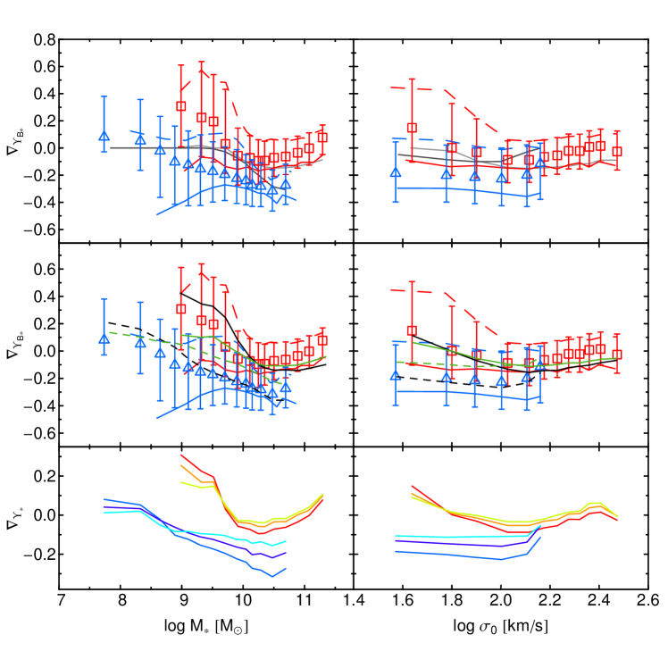
Figure 3: $M/L$ gradients as a function of stellar mass (left) and velocity dispersion (right). For ETGs a two fold trend in terms of both $M_{*}$ and $\sigma_{0}$ is found. LTGs present a steepening of the gradients with $M_{*}$, while they are independent of $\sigma_{0}$. Top: Default $B$-band gradients. The symbols are as in Fig. 2, with solid and dashed lines indicating galaxies with central $\rm age$ older and younger than $6\,\rm Gyr$, respectively. The light and dark grey lines are the results for ETGs and LTGs when no age gradients are assumed (adopting $\rm age=10\,\rm Gyr$). Middle: Default $B$-band gradients, symbols are as panels above. Black and green lines are the medians obtained using the $\mbox{$M/L$}-(g-r)$ and $\mbox{$M/L$}-(u-g)$ relations from B03, continue and dashed are for ETGs and LTGs. Bottom: Average gradients using different bandpasses: $B$ (red and blue lines for ETGs and LTGs, respectively), $V$ (orange and violet) and $i$ (yellow and cyan).

3.2 Trends with stellar mass and velocity dispersion

The trends of $\nabla_{\rm\tiny\mbox{$\Upsilon_{*}$}}$ with stellar mass and velocity dispersion are shown in the top panels of Fig. 3. As with the trend of colour and metallicity gradients with mass (see comments in §1 also T+10), we find that LTGs have a decreasing trend with mass and show $\nabla_{\rm\tiny\mbox{$\Upsilon_{*}$}}$$>0$ for $\log\mbox{$M_{*}$}/\mbox{$M_{\odot}$}\mathrel{\hbox to0.0pt{\lower 3.5pt\hbox{\hskip 0.5pt$\sim$}\hss}\raise 0.5pt\hbox{$<$}}9$ and $\nabla_{\rm\tiny\mbox{$\Upsilon_{*}$}}$$<0$ at larger masses. In contrast, ETGs have positive $\mbox{$\nabla_{\rm\tiny\mbox{$\Upsilon_{*}$}}$}\sim 0.25$ at low masses, which decreases down to a minimum of $\mbox{$\nabla_{\rm\tiny\mbox{$\Upsilon_{*}$}}$}\sim-0.1$ at $\log\mbox{$M_{*}$}/\mbox{$M_{\odot}$}\sim 10.3$ and then invert the trend, with the most massive ETGs having gradients around zero or slight positive. When plotted as a function of velocity dispersion, the $\nabla_{\rm\tiny\mbox{$\Upsilon_{*}$}}$ run with $\sigma_{0}$ is generally flatter, with LTGs having no trend and ETGs showing a two-fold trend with a minimum around $\log\mbox{$\sigma_{0}$}=2.1$ km/s and a mild increase toward the low and high $\sigma_{0}$ sides, always staying consistent with $\nabla_{\rm\tiny\mbox{$\Upsilon_{*}$}}$$\mathrel{\hbox to0.0pt{\lower 3.5pt\hbox{\hskip 0.5pt$\sim$}\hss}\raise 0.5pt\hbox{$<$}}0$.

Since galaxies are morphologically selected by using criteria on concentration and S$\rm\acute{e}$rsic index, the steeper gradients found for LTGs when compared with ETGs indicate a sequence in terms of such structural parameters. In fact, at fixed mass, galaxies with lower $C$ or $n$ have steeper colour and $M/L$ gradients.

As observed for the stellar population gradients (see T+10), the central age is responsible for much of the scatter of the trends versus mass and velocity dispersion, which is illustrated by the median distribution for centrally old ($>6\,\rm Gyr$) and young ($<6\,\rm Gyr$) galaxies in Fig. 3. In particular, young LTGs have almost null gradients, while the oldest ones have very steep values of $\mbox{$\nabla_{\rm\tiny\mbox{$\Upsilon_{*}$}}$}\sim-0.3$ to $-0.4$. ETGs show a similar but offset effect. Older ETGs have slightly negative values of $\sim-0.1$, while the younger ones have steep positive $\mbox{$\nabla_{\rm\tiny\mbox{$\Upsilon_{*}$}}$}\sim 0.5$ at very low masses, decreasing to $\sim 0.1$ at larger masses.

As a comparison, we also show in Fig. 3 (top panels) the results when galaxy colours are fitted to a synthetic spectral model which has no age gradient (fixed $\rm age=10\,\rm Gyr$). In this case, LTGs have $\nabla_{\rm\tiny\mbox{$\Upsilon_{*}$}}$ which are null up to $\log\mbox{$M_{*}$}/\mbox{$M_{\odot}$}\sim 9.5$, and decrease at larger masses, while gradients in ETGs show a milder trend when compared with the reference fit. When plotted versus $\sigma_{0}$  both LTGs and ETGs have similar $\nabla_{\rm\tiny\mbox{$\Upsilon_{*}$}}$ $\sim-0.1$ for all velocity dispersions. Note that these results are consistent with what was found for the older galaxies in the reference fit. We also compare our results with g-band $M/L$s derived from B03. As an example we plot the median lines derived using the $\mbox{$M/L$}-(g-r)$ and $\mbox{$M/L$}-(u-g)$ relations for both ETGs and LTGs. The trends with $M_{*}$ and velocity dispersion are qualitatively unchanged, but some differences emerge since the $M/L$s from each B03 relation are derived using different colours, which probe different wavelength spectral regions. The $M/L$s obtained using the $g-r$ colours seems to resemble our trends for LTGs, while the agreement is poorer when $u-g$ is used. For ETGs our trend is between the two B03 results at low mass, while the $M/L$ from $u-g$ is a little bit better at large mass.

We have also checked the effect of the waveband adopted for the $M/L$ ratios in the bottom panels of Fig. 3. Here, the $B$-band $M/L$ gradients are compared to the ones in $V$- and $i$-band. Except for the most massive ETGs, in general the $M/L$ gradients tend to become shallower (closer to zero) when using redder bands. Also, the trends with mass and velocity dispersion become weaker. Thus, redder bands, which are less affected by dust extinction and trace the older and metal-richer stellar populations in galaxies, tend to be less dependent on the existence of gradients in colour and stellar population parameters. Extending such analyzing into the NIR bands should find $M/L$ gradients increasingly approaching zero.

From the preceding results, we can see that although the age gradient is generally the driving parameter behind the $M/L$ gradient, this conclusion can vary depending on galaxy type, mass and central age. We summarize the gradients for different galaxy subsamples in Table 3, noting also which of the stellar parameters drives the $M/L$ gradient.

Table 3: $M/L$, age and metallicity gradients for subpopulations of galaxy type, stellar mass and central age. In (parentheses) we note whether the age or metallicity gradient drives the $M/L$ gradient.

LTGs	$\log\mbox{$M_{*}$}/\mbox{$M_{\odot}$}\mathrel{\hbox to0.0pt{\lower 3.5pt\hbox{\hskip 0.5pt$\sim$}\hss}\raise 0.5pt\hbox{$<$}}9$	$\log\mbox{$M_{*}$}/\mbox{$M_{\odot}$}~{}\hbox to0.0pt{$>$\hss}{\lower 4.30554pt\hbox{$\sim$}}9$
Young	$\mbox{$\nabla_{\rm\tiny\mbox{$\Upsilon_{*}$}}$}>0$; $\mbox{$\nabla_{\rm age}$}>0$; $\mbox{$\nabla_{\rm Z}$}\mathrel{\hbox to0.0pt{\lower 3.5pt\hbox{\hskip 0.5pt$\sim$}\hss}\raise 0.5pt\hbox{$<$}}0$	$\mbox{$\nabla_{\rm\tiny\mbox{$\Upsilon_{*}$}}$}<0$; $\mbox{$\nabla_{\rm age}$}>0$; $\mbox{$\nabla_{\rm Z}$}<0$
	(age)	(metallicity)
Old	$\mbox{$\nabla_{\rm\tiny\mbox{$\Upsilon_{*}$}}$}<0$; $\mbox{$\nabla_{\rm age}$}<0$; $\mbox{$\nabla_{\rm Z}$}\mathrel{\hbox to0.0pt{\lower 3.5pt\hbox{\hskip 0.5pt$\sim$}\hss}\raise 0.5pt\hbox{$<$}}0$	$\mbox{$\nabla_{\rm\tiny\mbox{$\Upsilon_{*}$}}$}<0$; $\mbox{$\nabla_{\rm age}$}\mathrel{\hbox to0.0pt{\lower 3.5pt\hbox{\hskip 0.5pt$\sim$}\hss}\raise 0.5pt\hbox{$<$}}0$; $\mbox{$\nabla_{\rm Z}$}<0$
	(age)	(metallicity)
ETGs	$\log\mbox{$M_{*}$}/\mbox{$M_{\odot}$}\mathrel{\hbox to0.0pt{\lower 3.5pt\hbox{\hskip 0.5pt$\sim$}\hss}\raise 0.5pt\hbox{$<$}}10$	$\log\mbox{$M_{*}$}/\mbox{$M_{\odot}$}~{}\hbox to0.0pt{$>$\hss}{\lower 4.30554pt\hbox{$\sim$}}10$
Young	$\mbox{$\nabla_{\rm\tiny\mbox{$\Upsilon_{*}$}}$}>0$; $\mbox{$\nabla_{\rm age}$}>0$; $\mbox{$\nabla_{\rm Z}$}~{}\hbox to0.0pt{$>$\hss}{\lower 4.30554pt\hbox{$\sim$}}0$	$\mbox{$\nabla_{\rm\tiny\mbox{$\Upsilon_{*}$}}$}>0$; $\mbox{$\nabla_{\rm age}$}>0$; $\mbox{$\nabla_{\rm Z}$}<0$
	(age)	(age)
Old	$\mbox{$\nabla_{\rm\tiny\mbox{$\Upsilon_{*}$}}$}<0$; $\mbox{$\nabla_{\rm age}$}\mathrel{\hbox to0.0pt{\lower 3.5pt\hbox{\hskip 0.5pt$\sim$}\hss}\raise 0.5pt\hbox{$<$}}0$; $\mbox{$\nabla_{\rm Z}$}~{}\hbox to0.0pt{$>$\hss}{\lower 4.30554pt\hbox{$\sim$}}0$	$\mbox{$\nabla_{\rm\tiny\mbox{$\Upsilon_{*}$}}$}<0$; $\mbox{$\nabla_{\rm age}$}\sim 0$; $\mbox{$\nabla_{\rm Z}$}<0$
	(age)	(metallicity)

4 Discussions and conclusions

In this paper we have investigated the correlation between $M/L$ gradients and stellar mass or velocity dispersion for a large sample of local galaxies from SDSS. The gradients $\nabla_{\rm\tiny\mbox{$\Upsilon_{*}$}}$ have been derived by the fitting of synthetic spectral models to observed optical colours. We have used Monte Carlo simulations to check that the optical-only wavelength baseline should not dramatically affect the results compared to including near-infrared and ultraviolet data. This conclusion is encouraging in view of future studies of higher redshift galaxies which are generally observed in rest-frame optical bands. Anyway, future analysis in local samples, relying on near-IR and/or UV data would be able to give further details about the degeneracies and systematics affecting stellar fitting.

We have found that there exists a tight positive correlation between $\nabla_{\rm\tiny\mbox{$\Upsilon_{*}$}}$ and colour gradients which is not surprising because of the well known $M/L$-colour correlations (e.g., Bell & de Jong 2001; B03). We have found that $M/L$ is a decreasing function of stellar mass in LTGs, while a two-fold trend is found for ETGs (for both stellar mass and velocity dispersion), in agreement with the trends of colour gradients discussed in T+10. Similar results are obtained using the $M/L$-colour relations from B03, which, although easy to use, do not give information about stellar population parameters. Thus, the novelty of our approach resides in our ability to check how $\nabla_{\rm\tiny\mbox{$\Upsilon_{*}$}}$ gradients are driven by variations in metallicity or age. In general, we have found that age is most important, but that metallicity becomes more important in many high-mass galaxies.

This picture does not change dramatically if $M/L$ gradients are calculated in redder bands ($V$- and $i$-bands rather than $B$). In these cases $\nabla_{\rm\tiny\mbox{$\Upsilon_{*}$}}$ are shallower and the trends with stellar mass and velocity dispersion become milder (Fig. 3). These results suggest that $M/L$ estimates from red or infrared bands would not depend on galactocentric radius, since the radiation emitted by stellar populations in these spectral regions is more homogenous.

This is the first work to derive $M/L$ gradients 1) from observations of a large galaxy sample and 2) using a direct stellar population analysis approach. The only point of comparison is the work by Portinari & Salucci (2010) in a sample of spiral galaxies, where negative $M/L$ gradients were found to be important in modelling rotation curves.

We may explain some of our observed trends through physical mechanisms as follow. Starting from low-mass systems, centrally-young LTGs have age increasing with radius while metallicity decreases, which can be due to the presence of a gas inflow which allows the formation of younger stars in the centre with a smaller $M/L$. Centrally-old LTGs have age decreasing with radius which implies recent outer star formation with a similar metallicity to the centre. Here the central star formation might have been quenched by SNe which have expelled metals to larger radii (where the younger stars drive a smaller $M/L$). Centrally-young ETGs have positive age, metallicity and $M/L$ gradients, and may hosting expanding shells (Mori et al. 1997). Centrally-old ETGs show mild negative age gradients and very shallow positive metallicity gradients, similarly to the old LTGs thus again suggesting SNe having played a role.

The more massive centrally-young LTGs have decreasing $M/L$ with radius, but also strong negative $\nabla_{\rm Z}$, thus the new stars formed inside the core ($\nabla_{\rm age}$$>0$) have higher metallicity and $M/L$. This might be due to recycled gas from SNe or AGN which is falls back to the centre due to the deep potential wells and produces a rejuvenated stellar population. In centrally-young ETGs, on the other hand, the younger stars formed later in the centres (i.e. with positive age gradients) and with higher metallicities, possibly because of a central burst of star formation in “wet” mergers (e.g. Rothberg & Joseph 2004; Hopkins et al. 2009; Hopkins et al. 2010; T+10). Centrally-old LTGs and ETGs show very similar behaviors, which seem compatible with merging events that largely wash out any age gradients (and the $\nabla_{\rm Z}$ in ETGs), and may produce coeval metallicities in the outer regions of the LTGs. In both cases the net effect is that metallicity is the main driver of the strong negative $\nabla_{\rm\tiny\mbox{$\Upsilon_{*}$}}$ in LTGs and of the weak negative $\nabla_{\rm\tiny\mbox{$\Upsilon_{*}$}}$ of the massive ETGs (in any). Thus, the physical mechanisms that can account for the observations outlined in Tab. 3 seem consistent with the evolutionary scenario discussed in §1.

In particular, the two-fold trend of ETGs in Fig. 3, with a minimum around $\log\mbox{$M_{*}$}/\mbox{$M_{\odot}$}=10.3$ is mirrored by the colour and stellar population gradients as in Fig. 1 (and T+10) and found also in other works (Rawle et al. 2010; Spolaor et al. 2009, 2010). The characteristic mass agrees well with the typical mass scale break for star forming and passive systems (Kauffmann et al. 2003), for “bright” and “ordinary” galaxies (Capaccioli et al. 1992a; Graham & Guzm$\rm\acute{a}$n 2003; Graham et al. 2003; Trujillo et al. 2004; 2009), or for cold and hot flow (shock heating; Dekel & Birnboim 2006).

Following the main conclusions in T+10, quasi-monolithic collapse and supernovae feedback could be the main drivers of the decreasing $\nabla_{\rm\tiny\mbox{$\Upsilon_{*}$}}$-$M_{*}$ trends in LTGs and low mass ETGs (Larson 1974; Kawata 2001, Kawata & Gibson 2003), while the increasing trends in massive ETGs could be explained by the heightened importance of mergers and AGN feedback (2004; Sijacki et al. 2007; Hopkins et al. 2009).

$M/L$ gradients are expected from simulations of galaxy formation and evolution. E.g. Boissier & Prantzos (1999) found in chemo-dynamical simulations of spiral galaxies that the central regions ($<12\,\rm kpc$) have steep negative $M/L$ gradients, becoming flatter at larger radii. High-redshift ($z\sim 2$) merger remnants simulated by Wuyts et al. (2010) showed time-dependent negative $M/L$ as a consequence of redder cores in redder galaxies (similarly to observations of local galaxies in T+10). $M/L$ gradients were also predicted for merger remnants by Hopkins et al. (2010), who stressed that the effective radius derived from the $B$-band light would increase with time (by $\sim$ 10%) simply because of stellar population gradients. This effect is important for conclusions about stellar densities and related dynamical implications (e.g. for the fundamental plane). Similarly van Dokkum (2008) argued that the existence of such gradients can imply that the observed quiescent galaxies at large redshift may be of an order or magnitude more dense than previously found from observations.

The $M/L$ gradients present a general complication for estimates of the dark matter distribution in galaxies. Portinari & Salucci (2010) found that for spiral galaxies, including $M/L$ gradients would change the fits to circular velocity curves but not produce strong effects on the inferred dark matter density parameters. To our knowledge, this issue has not been addressed in the literature for early-type galaxies, and it is beyond the scope of the present paper to do so in any detail. In particular, we have studied the stellar population gradients only inside 1 $R_{\rm eff}$, while the gradients out to $\sim$ 5 $R_{\rm eff}$ could be important for dark matter analyses (e.g. Napolitano et al. 2005, 2009, 2011). Assuming that the gradients do not change radically outside $\sim$ 1 $R_{\rm eff}$, for the massive ETGs generally studied with lensing or dynamics ($\mbox{$\sigma$}_{0}~{}\hbox to0.0pt{$>$\hss}{\lower 4.30554pt\hbox{$\sim$}}$ 150 km s^-1), we would expect the stellar $M/L$ gradients to be mild (see Fig. 3), and to not strongly affect the dark matter estimates.

A final issue is that until now, we have assumed that the IMF is invariant. If there are galaxy-to-galaxy variations in the IMF (see e.g. van Dokkum & Conroy 2010, 2011; Gunawardhana et al. 2011), then the stellar $M/L$ values are changed only by a constant multiplicative value, and the implied gradients remain unchanged. However, IMF variations if real would then likely exist within galaxies owing to variations in stellar populations. Indeed, there have been many suggestions that stars forming at early times had a non-standard IMF (e.g. Larson 2005; Klessen et al. 2007; van Dokkum 2008; Davé 2008; Holden et al. 2010).

One study of nearby ETGs suggested that systems with older stars within 1 $R_{\rm eff}$ have “lighter” (closer to Chabrier than Salpeter) IMFs (Napolitano, Romanowsky & Tortora, 2010). This would imply that positive and negative age gradients would decrease and increase the stellar $M/L$ gradients, respectively. Revisiting Fig. 3, the gradients for the centrally-young objects would decrease and the centrally old objects would increase, possibly reducing and even eliminating the age-related scatter in the gradient trends.

Another scenario would be if the central regions of massive ETGs have “higher-mass” IMFs than standard (van Dokkum & Conroy 2011), while the outer regions have accreted galaxies with more “normal” IMFs (e.g. Kroupa 2001 or Chabrier 2003). This would decrease these galaxies’ stellar $M/L$ gradients, although it is not clear how this effect would relate to age and metallicity trends.

In future analyses, we plan to analyze stellar $M/L$ profiles out to a few $R_{\rm eff}$, and analyze the impact of $M/L$ gradients on dark matter profile inferences, which may be compared to $\Lambda$CDM (e.g. Navarro, Frenk & White 1996). We will also consider the (probably small) adjustments implied for central dark matter inferences (e.g. Tortora et al. 2010b). Dust effects will further be examined: dust is not important for metallicity gradients (see T+10) but could affect age and thereby $M/L$ gradients, particularly for intermediate-mass ETGs.

References

- Auger et al. (2010) Auger M. W., Treu T., Bolton A. S., Gavazzi R., Koopmans L. V. E., Marshall P. J., Moustakas L. A., Burles, S. 2010, ApJ, 724, 511
- Bekki & Shioya (1999) Bekki, K., & Shioya, Y. 1999, ApJ, 513, 108
- Bell & de Jong (2001) Bell E. F. & de Jong R. S. 2001, ApJ, 550, 212
- Bell et al. (2003) Bell E. F., McIntosh D. H., Katz N., Weinberg M. D. 2003, ApJS, 149, 289 (B03)
- Blanton et al. (2005) Blanton M. R. et al. 2005, AJ, 129, 2562 (B05)
- Boissier & Prantzos (1999) Boissier S., Prantzos N. 1999, MNRAS, 307, 857
- Bruzual & Charlot (2003) Bruzual, A. G. & Charlot, S. 2003, MNRAS, 344, 1000
- Capaccioli et al. (1992a) Capaccioli M., Caon N. & D’Onofrio M. 1992, MNRAS, 259, 323
- Chabrier (2001) Chabrier, G. 2001, ApJ, 554, 1274
- Chabrier (2003) Chabrier, G. 2003, PASP, 115, 763
- Davé (2008) Davé, R. 2008, MNRAS, 385, 147
- Dekel & Birnboim (2006) Dekel A., & Birnboim Y. 2006, MNRAS, 368, 2
- den Brok et al. (2011) den Brok, M. et al. 2011, MNRAS, 414, 3052
- Di Matteo et al. (2009) di Matteo P., Pipino A., Lehnert M. D., Combes F., Semelin B. 2009, A&A, 499, 427
- Gallazzi et al. (2005) Gallazzi, A. et al. 2005, MNRAS, 362, 41
- Gunawardhana et al. (2011) Gunawardhana, M. L. P., et al. 2011, MNRAS, in press, arXiv:1104.2379
- Gargiulo, Saracco & Longhetti (2011) Gargiulo A., Saracco P., Longhetti M. 2011, MNRAS, 412.1804
- Gonzalez-Perez et al. (2011) Gonzalez-Perez V., Castander F. J. & Kauffmann G. 2011, MNRAS, 411, 1151
- Graham & Guzmn (2003) Graham A. W., Guzmn R., 2003, AJ, 125, 2936
- Graham et al. (2003) Graham A.W., Erwin P., Trujillo I., Asensio Ramos A., 2003, AJ, 125, 2951
- Holden et al. (2010) Holden, B. P., van der Wel, A., Kelson, D. D., Franx, M., & Illingworth, G. D. 2010, ApJ, 724, 714
- Hopkins et al. (2009) Hopkins P. F., Cox T. J., Dutta S. N., Hernquist L., Kormendy J., & Lauer T. R. 2009, ApJS, 181, 135
- Hopkins et al. (2010) Hopkins P.F., Bundy K. Hernquist L., Wuyts S., Cox T. J. 2010, MNRAS, 401, 1099
- Jarrett et al. (2003) Jarrett T. H., Chester T., Cutri R., Schneider S. E., Huchra J. P. 2003, AJ, 125, 525
- Kauffmann et al. (2003) Kauffmann G. et al. 2003, MNRAS, 341, 54
- Kawata (2001) Kawata D. 2001, ApJ, 558, 598
- Kawata & Gibson (2003) Kawata D. & Gibson B. K. 2003, MNRAS, 340, 908
- Klessen et al. (2007) Klessen, R. S., Spaans, M., & Jappsen, A.-K. 2007, MNRAS, 374, L29
- (29) Kobayashi C. 2004, MNRAS, 347, 740
- (30) Kormendy J., Fisher D. B., Cornell M. E., Bender R., 2009, ApJS, 182, 216
- Kroupa (2001) Kroupa P., 2001, MNRAS, 322, 231
- (32) Kuntschner H. et al. 2010, MNRAS, 408, 97
- (33) La Barbera F., et al. 2005, ApJ, 626, 19
- Larson (1974) Larson R. B., 1974, MNRAS, 166, 585
- Larson (1975) Larson R. B., 1975, MNRAS, 173, 671
- Larson (2005) Larson, R. B. 2005, MNRAS, 359, 211
- Maraston (2005) Maraston C. 2005, MNRAS, 362, 799
- Martin et al. (2005) Martin D. C. et al., 2005, ApJ, 619, L1
- Matteucci (1994) Matteucci F. 1994, A&A, 288, 57
- Mihos & Hernquist (1994) Mihos J. C. & Hernquist L., 1994, ApJ, 437, L47
- Mori et al. (1997) Mori, M. et al. 1997, ApJ, 478, 21
- Napolitano et al. (2005) Napolitano, N. R., et al. 2005, MNRAS, 357, 691
- Napolitano et al. (2009) Napolitano, N. R., Romanowsky, A. J., Coccato, L., et al. 2009, MNRAS, 393, 329
- Napolitano, Romanowsky & Tortora (2010) Napolitano N. R., Romanowsky A. J. & Tortora, C. 2010, MNRAS, 405, 2351
- Napolitano et al. (2011) Napolitano N. R. et al. 2011, MNRAS, 411, 2035
- Navarro, Frenk & White (1996) Navarro, J. F., Frenk, C. S., & White, S. D. M. 1996, ApJ, 462, 563
- Portinari & Salucci (2010) Portinari L. & Salucci P. 2010, A&A, 521, 82
- Pipino et al. (2008) Pipino A., D’Ercole A. & Matteucci F. 2008, A&A, 484, 679
- Pipino et al. (2010) Pipino A., D’Ercole A., Chiappini C. & Matteucci F. 2010, MNRAS, 407, 1347
- Rawle et al. (2010) Rawle T. D., Smith R. J. & Lucey J. R. 2010, MNRAS, 401, 852
- Romanowsky et al. (2009) Romanowsky, A. J., Strader, J., Spitler, L. R., Johnson, R., Brodie, J. P., Forbes, D. A., & Ponman, T. 2009, AJ, 137, 4956
- Rothberg & Joseph (2004) Rothberg B., Joseph R. D. 2004, AJ, 128, 2098
- Salpeter (1955) Salpeter, E.E. 1955 ApJ, 121, 161
- Snchez-Blzquez et al. (2007) Snchez-Blzquez P., Forbes D. A., Strader J., Brodie J., Proctor R. 2007, MNRAS, 377, 759
- Sijacki et al. (2007) Sijacki D. et al. 2007, MNRAS, 380, 877
- Spolaor et al. (2009) Spolaor, M., Proctor, R. N., Forbes, D. A., Couch, W. J. 2009, ApJ, 691, 138
- Spolaor et al. (2010) Spolaor M., Kobayashi C., Forbes D. A., Couch, W. J., Hau G. K. T. 2010, MNRAS, 408, 272
- Tamura et al. (2000) Tamura, N., et al. 2000, AJ, 119, 2134
- Tamura & Ohta (2000) Tamura, N., & Ohta, K. 2000, AJ, 120, 533
- Tamura & Ohta (2003) Tamura, N., & Ohta, K. 2003, AJ, 126, 596
- Tortora et al. (2009) Tortora C. et al. 2009, MNRAS, 396, 1132
- Tortora et al. (2009b) Tortora C. et al. 2009b, MNRAS, 396, 61
- Tortora et al. (2010a) Tortora C., Napolitano N. R., Cardone V. F., Capaccioli M., Jetzer Ph., Molinaro R. 2010a, MNRAS, 407, 144
- Tortora et al. (2010b) Tortora C., Napolitano N. R., Romanowsky A. J., Jetzer P. 2010b, ApJ, 721, 1
- Tortora et al. (2011) Tortora C., Romeo A. D., Napolitano N. R., Antonuccio-Delogu V., Meza A., Sommer-Larsen J., Capaccioli M. 2011, MNRAS, 411, 627
- Trujillo et al. (2004) Trujillo I., Erwin P., Asensio Ramos A., Graham A. W., 2004, AJ, 127, 1917
- van Dokkum (2008) van Dokkum, P. G. 2008, ApJ, 674, 29
- van Dokkum & Conroy (2010) van Dokkum, P. G., & Conroy, C. 2010, Nature, 468, 940
- van Dokkum & Conroy (2011) van Dokkum, P., & Conroy, C. 2011, ApJ, 735L, 13
- Worthey (1994) Worthey G. 1994, ApJS, 95, 107
- Wuyts et al. (2010) Wuyts S., Cox T. J., Hayward C. C., Franx M., Hernquist L., Hopkins P. F., Jonsson P., van Dokkum P. G. 2010, ApJ, 722, 1666