Quantum Filtering (Quantum Trajectories) for Systems Driven by Fields in Single Photon and Superposition of Coherent States

Abstract

We derive the stochastic master equations, that is to say, quantum filters, and master equations for an arbitrary quantum system probed by a continuous-mode bosonic input field in two types of non-classical states. Specifically, we consider the cases where the state of the input field is a superposition or combination of: (1) a continuous-mode single photon wave packet and vacuum, and (2) any continuous-mode coherent states.

I Background and Motivation

The production and verification of non-classical states of light, such as single-photon states LvoAicBen01 and superpositions of coherent states (also known as Schrödinger cat states) NeeNieHet06 ; OurTuaLau06 ; OurHyuTua07 , has become routine. In particular, the production of single photon states has been achieved in a variety of experimental architectures such as: cavity quantum electrodynamics (QED) KuhHenRem02 ; McKBocBoo04 , quantum dots in semiconductors YuaKarSte02 , and recently in circuit QED jay . Such non-classical states have been considered in connection with quantum computing KLM01 ; RalGilMil03 and secure communication GisRibTit02 over quantum networks CirZolKim97 .

A basic problem in quantum optics concerns the extraction of information about a system of interest (two-level atom, cavity mode, etc) from light scattered by the system, Figure 1. Based on measurements of the scattered, or output, light, one can determine a conditional state from which one can make estimates of observables of the system. A general approach to estimation problems of this kind, called filtering problems, was developed by Belavkin Belavkin1 -BarBel91 within a framework of continuous non-demolition quantum measurement in the case where the input probe field, $B(t)$ in Figure 1, is a quantum white noise with vacuum state (or more generally Gaussian state, see GSobolev04 - GK10 ). Belavkin’s formulation, which generalizes the classical nonlinear filtering theory Stratonovich , is quite general. For example, in the schematic representation of a continuous measurement process shown in Figure 1, the measurement signal $Y(t)$ produced by a detector (e.g. photon counter or homodyne detector) may be the number of quanta in the output field, or alternatively it may be a quadrature of the output field.

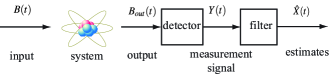
Figure 1: A schematic representation of a continuous measurement process, where the measurement signal produced by a detector is filtered to produce estimates $\hat{X}(t)=\pi_{t}(X)=\mathrm{tr}[\rho(t)X]$ of system operators $X$ at time $t$.

One obtains a filtering equation which is a stochastic differential equation of the state $\varrho(t)$ conditioned on $Y(t)$: in the later terminology employed in quantum optics, the output is referred to as a quantum trajectory and the filtering equation as a stochastic master equation CarBook93 ; DalCasMol92 ; GisPer92 . Averaging over the measured output is equivalent to a non-selective measurement, and the corresponding state will satisfy the corresponding master equation. The choice of detection scheme on the output field determines the particular selective evolution, usually referred to as an unravelling of the master equation in quantum optics. To date, quantum trajectories and quantum filtering have only been developed for input fields that are in a Gaussian state, with specific cases being coherent state fields (this includes vacuum fields as special case), thermal fields, and squeezed fields GarCol85 ; DumParZol92 ; GarZol00 . While the resulting equations allow us to estimate non-commutating observables of the monitored system, the Gaussian nature of the inputs ensure that they appear formally similar to the classical equations. The aim of the present paper is to extend the theory to classes of non-classical inputs.

In this article we extend Belavkin’s quantum filtering theory and the input-output theory of quantum optics GarCol85 ; CarBook93 to non-Gaussian continuous-mode states $\rho_{\text{field}}$ which are superpositions or combinations of

• a continuous-mode single photon and vacuum, and

• continuous-mode coherent states, i.e. continuous-mode cat-states.

The problem to be tackled here is to derive the master and stochastic master equations for a “system”$\otimes$“field” with initial state $\rho_{0}\otimes\rho_{\text{field}}$ and unitary evolution process $U\left(t\right)$ when the field state is one of the states above. To make the problem tractable, we seek a larger representation of the form “extended system”$\otimes$“field” where

$$\text{``extended system''=``ancilla''}\otimes\text{``system''}$$

such that, for all system observables $X$,

$$\text{{tr}}_{\text{system}\otimes\text{field}}\left\{\rho_{0}\otimes\rho_{\text{field}}\,U\left(t\right)^{{\dagger}}\left(X\otimes I\right)U\left(t\right)\right\}$$

$$=\text{{tr}}_{\text{ancilla}\otimes\text{system}\otimes\text{field}}\big{\{}\rho_{a}\otimes\rho_{0}\otimes P_{\text{vac}}$$

$$\tilde{U}\left(t\right)^{{\dagger}}\left(R\left(t\right)\otimes X\otimes I\right)\tilde{U}\left(t\right)\big{\}}$$ (1)

where $\tilde{U}\left(t\right)$ is a unitary evolution process coupling the ancilla, system, and field, $\rho_{a}$ is a fixed state of the ancilla, $P_{\text{vac}}=|0\rangle\langle 0|$ is the vacuum state (projection) for the continuous-mode field, and $R\left(t\right)$ is some process taking values in the observables of the ancilla. The filtering problem may then be solved for the extended system with reference to the vacuum state for the field using traditional techniques.

The extension to single photon states is interesting for foundational reasons TanWalCol91 as well as the aforementioned technological reasons KLM01 . Likewise, quantum filtering for cat states is of foundational importance, while practical uses would be towards quantum enhanced metrology WisMilBook . One possible application would be to quantum enhanced metrology of a time varying parameter MilMunNem02 ; MunRalGla04 .

This article is structured as follows. In Section II we review standard input-output theory. Specifically we consider the idealized quantum white-noise model of a quantum stochastic differential equation (QSDE) and use it to derive the master equations and quantum trajectories for Gaussian fields. Then we review a general parametrization to specify the system environment coupling for input-output systems. Using this parametrization we review the methods, recently introduced YanKim03_1 ; GouJam09a ; GouJam09b , to simplify and formalize the network theory of cascaded open quantum systems and quantum feedback networks.

Section III is focused on deriving the master equation and stochastic master equation (quantum filter) driven by continuous-mode single photon wave packets. We generalize the single photon filter to any superposition or combination of single photon and vacuum input field. The system that is probed is left arbitrary so in general our filter can apply to qubits, qudits and mechanical oscillators. As an example we calculate the single photon filter for a two level atom (or qubit) dispersively coupled to the field. We derive the trajectories for both a homodyne type measurement and a photon counting measurement.

In Section IV we present the extension to superpositions of coherent states. We derive the cat-state-filter for an arbitrary quantum system and an arbitrary cat state. Again we illustrate the filtering equations with a qubit system and homodyne and photon counting measurements.

In Section V we conclude and discuss our future research and some open questions.

Notation The commutator and anti-commutator will be denoted as $[A,B]=AB-BA$ and $[A,B]_{+}=AB+BA$, respectively. We set $\mathcal{D}_{A}B\equiv A^{{\dagger}}BA-\frac{1}{2}(A^{{\dagger}}AB+BA^{{\dagger}}A)$ and $\mathcal{D}_{A}^{\star}B\equiv ABA^{{\dagger}}-\frac{1}{2}(A^{{\dagger}}AB+BA^{{\dagger}}A)$.

The scattering, coupling and Hamiltonian operators describing a given Markovian open system coupling will be written as a triple $G=(S,L,H)$, to be explained in more detail in Section II.1, and this provides an operator-valued parameterization of the system. The associated superoperators are

$$\mathit{Lindbladian:} \,\mathcal{L}_{G}X\equiv-i[X,H]+\mathcal{D}_{L}X,$$

$$\mathit{Liouvillian:} \,\mathcal{L}_{G}^{\star}\rho\equiv-i[H,\rho]+\mathcal{D}_{L}^{\star}\rho,$$

and note that, for traceclass $\rho$ and bounded $X$,

$$\mathrm{tr}\{\rho\mathcal{L}_{G}X\}=\mathrm{tr}\{X\mathcal{L}_{G}^{\star}\rho\}.$$

II Models of Open Quantum Systems

In this section we briefly review quantum stochastic calculus (input-output theory) and quantum filtering (trajectories) for a system coupled to a heat bath modelled as a boson field in the vacuum state.

II.1 Input-Output Model Using QSDEs

Hudson and Parthasarathy HudPar84 ; Par92 showed how to dilate a dissipated completely positive semigroup evolution, with Lindblad generator, to a unitary model on the system space with a (Bose) Fock space ancilla. Here they developed an analogue to the Itō theory of stochastic integration with respect to creation, annihilation and scattering process $B^{{\dagger}}\left(t\right),B\left(t\right)$ and $\Lambda\left(t\right)$. They showed the existence and uniqueness of solutions to unitary quantum stochastic differential equations of the form

$$dU(t)= \biggl{\{}\left(S-1\right)d\Lambda\left(t\right)+LdB^{{\dagger}}(t)$$

$$-L^{{\dagger}}SdB(t)-(\mbox{$\frac{1}{2}$}L^{{\dagger}}L+iH)dt\biggr{\}}U(t).$$ (2)

where

$$G=\left(S,L,H\right)$$

consists of a unitary $S$ describing photon scattering phase, a bounded operator $L$ describing coupling to the creation mode of the field, and a bounded Hermitean operator $H$ describing the system Hamiltonian. (The result has been extended to non-bounded coefficients.) The increments are future pointing operator-valued Itō increment, that is $dB(t)\equiv B(t+dt)-B(t)$ is a forward of the quantum noise. In particular, we have. $[U(t),dB(t)]=[U(t),dB^{{\dagger}}(t)]=[U(t),d\Lambda(t)]=0$. The full quantum Itō table is

dt0000dB00dBdtdΛ00dΛdB†dB†0000.fragments fragmentsdt0000fragmentsdB00fragmentsdBfragmentsdtfragmentsdΛ00fragmentsdΛfragmentsdB†fragmentsdB†0000\begin{tabular}[]{l|llll}$\times$&$dt$&$dB$&$d\Lambda$&$dB^{{\dagger}}$\\ \hline\cr$dt$&0&0&0&0\\ $dB$&0&0&$dB$&$dt$\\ $d\Lambda$&0&0&$d\Lambda$&$dB^{{\dagger}}$\\ $dB^{{\dagger}}$&0&0&0&0\end{tabular}.

×dtdBdΛdB†×dtdBdΛdB† (3)

More generally, for quantum stochastic integral processes $X(t),Y(t)$, one has the Itō product rule

$$d(X(t)Y(t))=(dX(t))\,Y(t)+X(t)\,dY(t)+dX(t)\,dY(t).$$

Independently, Gardiner and Collett developed an equivalent quantum input-output theory GarCol85 ; GarZol00 based on Lehmann-Symanzik-Zimmermann scattering theory of Bose white noise processes. Formally one begins with singular fields satisfying

$$\left[b\left(t\right),b^{{\dagger}}\left(s\right)\right]=\delta\left(t-s\right),$$

with the connection to the regular processes being formally

$$B^{{\dagger}}\left(t\right) = \int_{0}^{t}b^{{\dagger}}\left(s\right)ds,\quad B\left(t\right)=\int_{0}^{t}b\left(s\right)ds,$$

$$\Lambda\left(t\right) = \int_{0}^{t}b^{{\dagger}}\left(s\right)b\left(s\right)ds.$$

The quantum stochastic calculus may then be understood as effectively arising through Wick ordering of the singular fields.

The multiple input version is relatively straightforward. We have $n$ independent inputs $b_{j}$ and with $B_{j}\left(t\right)=\int_{0}^{t}b_{j}\left(s\right)ds$, $\Lambda_{jk}\left(t\right)=\int_{0}^{t}b_{j}^{{\dagger}}\left(s\right)b_{k}\left(s\right)ds$, etc., we have

$$dU(t) =\left\{\sum_{jk}\left(S_{jk}-\delta_{jk}\right)d\Lambda_{jk}\left(t\right)+\sum_{j}L_{j}dB_{j}^{{\dagger}}(t)\right.$$

$$\left.-\sum_{jk}L_{j}^{{\dagger}}S_{jk}dB_{k}(t)-\biggl{(}\frac{1}{2}\sum_{j}L_{j}^{{\dagger}}L_{j}+iH\biggr{)}dt\right\}U(t),$$

where we now have parameterizing operators

$$S=\left(\begin{array}[]{ccc}S_{11}&\dots&S_{1n}\\ \vdots&\ddots&\vdots\\ S_{n1}&\dots&S_{nn}\end{array}\right),L=\left(\begin{array}[]{c}L_{1}\\ \vdots\\ L_{n}\end{array}\right),H$$

with $S$ unitary and $H$ self-adjoint. For simplicity we treat the case of a single input and output.

II.2 Heisenberg-Langevin Equations

The Heisenberg dynamics of arbitrary system operator $X$ is defined by transforming to the Heisenberg picture

$$j_{t}(X)=U^{\dagger}(t)(X\otimes I_{\mathrm{field}})U(t).$$

(We will usually drop the subscripts “system” and “field’ when there is no confusion.) From the quantum Itō product rule and table one deduces the QSDE for a system operator $j_{t}(X)=X(t)$: with all system operators transformed to the Heisenberg picture.

$$dj_{t}(X) =j_{t}(\mathcal{L}X)dt$$

$$+dB^{\dagger}(t)j_{t}(S^{\dagger}[X,L])+j_{t}([L^{\dagger},X]S)dB(t)$$

$$+j_{t}(S^{\dagger}XS-X)d\Lambda(t).$$ (4)

II.3 Derivation of the Master Equation

Suppose that the system is in an initial state $\rho(0)=\rho_{0}$ and that the joint state of the system and bath is $\rho_{0}\otimes P_{\text{vac}}$ where $P_{\text{vac}}=|0\rangle\langle 0|$ is projection onto the vacuum state of the field. The state of the system, $\varrho(t)$, obtained by averaging over the environment at a given time $t$ is then

$$\varrho(t)=\mathrm{tr}_{\text{field}}\left[U(t)(\rho_{0}\otimes P_{\text{vac}})U^{{\dagger}}(t)\right].$$ (5)

We wish to obtain a differential equation for the average of an observable $X$ of the system at time $t$:

$$\varpi_{t}\left(X\right) = \mathrm{tr}_{\text{system}\otimes\text{field}}\left\{j_{t}\left(X\right)\varrho_{0}\otimes P_{\text{vac}}\right\}$$

$$\equiv \mathrm{tr}_{\text{system}}\left\{\rho\left(t\right)X\right\},$$

and from the Heisenberg-Langevin equation (4) we have

$$d\varpi_{t}\left(X\right) = \mathrm{tr}_{\text{system}\otimes\text{field}}\left\{dj_{t}\left(X\right)\rho_{0}\otimes P_{\text{vac}}\right\}$$

$$= \mathrm{tr}_{\text{system}\otimes\text{field}}\left\{j_{t}\left(\mathcal{L}_{G}X\right)\rho_{0}\otimes P_{\text{vac}}\right\}dt,$$

as the increments $dB,dB^{{\dagger}},d\Lambda$ vanish in the vacuum state. We therefore obtain the equation

$$\frac{d\varpi_{t}\left(X\right)}{dt}=\varpi_{t}\left(\mathcal{L}_{G}X\right),\quad\varpi_{0}\left(X\right)=\mathrm{tr}_{\text{system}}\left\{\rho_{0}X\right\}$$

which may then be expressed as the master equation

$$\frac{d\varrho(t)}{dt}=\mathcal{L}_{G}^{\star}\varrho(t)\equiv-i[H,\varrho(t)]+\mathcal{D}_{L}^{\star}\varrho(t),$$ (6)

with initial data $\rho_{0}$. Note that the master equation (6) is a consequence of the QSDE model.

II.4 The Input-Output Relations

The output field $B_{\text{out}}$ is obtained from the input by moving into the Heisenberg picture:

$$B_{\text{out}}\left(t\right) = U\left(t\right)^{{\dagger}}\left(I_{\text{system}}\otimes B\left(t\right)\right)U\left(t\right)$$

$$\equiv U\left(\tau\right)^{{\dagger}}\left(I_{\text{system}}\otimes B\left(t\right)\right)U\left(\tau\right)$$

for any $\tau\geq t$. Again from the quantum Itō calculus we find

$$dB_{\text{out}}\left(t\right)=j_{t}\left(S\right)dB\left(t\right)+j_{t}\left(L\right)dt.$$ (7)

Note that the output field again satisfies the canonical commutation relations.

Figure 2: An open quantum system. The input field (before interaction) is represented by the operator $B(t)$ and output field (after interaction) is denoted by $B_{\mathrm{out}}(t)$.

II.5 Derivation of the Quantum Filter (Stochastic Master Equation) - Quadrature Case

We suppose that we continuously monitor the quadrature phase using perfect (100% efficiency) homodyne detection. This entails measurement, for each $t\geq 0$, of the field

$$Y(t) = B_{\mathrm{out}}(t)+B_{\mathrm{out}}^{{\dagger}}(t)$$

$$\equiv U\left(t\right)^{{\dagger}}\left(I_{\text{system}}\otimes Q\left(t\right)\right)U\left(t\right)$$

where $Q\left(t\right)=B\left(t\right)+B^{{\dagger}}\left(t\right)$. We note that the set of observables $\left\{Y\left(t\right):t\geq 0\right\}$ is self-commuting and we may simultaneously diagonalize (and measure!) all observables. At any time $t$, we may additionally estimate an observable that commutes with the observables up to time $t$. This includes observables $X\left(\tau\right)$ for $\tau\geq t$, since

$$\left[X\left(\tau\right),Y\left(t\right)\right]$$

$$= U\left(\tau\right)^{\ast}\left[X\otimes I_{\text{field}},I_{\text{system}}\otimes Q\left(t\right)\right]U\left(\tau\right)$$

$$\equiv 0\text{.}$$

This is the non-demolition property. Quantum filtering is the estimation of $j_{t}\left(X\right)$ based on observations of the output processes$\left\{Y\left(s\right):0\leq s\leq t\right\}$. Fig. 1 depicts the scenario we are considering. From the Itō calculus we see that

$$dY(t)=(L(t)+L^{{\dagger}}(t))dt+dQ(t).$$

Defining the expectation

$$\mathbb{E}[\cdot]=\mathrm{tr}\{\rho_{0}\otimes\rho_{\text{field}}\,(\cdot)\}$$

for a given state $\rho_{0}\otimes\rho_{\text{field}}$, we seek to minimize

$$\mathbb{E}[(\hat{X}(t)-j_{t}\left(X\right))^{2}]$$

over all observables $\hat{X}\left(t\right)$ in the algebra $\mathcal{Y}_{t}$ generated by $\left\{Y\left(s\right):0\leq s\leq t\right\}$. The minimizer is called the least-squares estimator for $X\left(t\right)$ given $\left\{Y\left(s\right):0\leq s\leq t\right\}$ and will be denoted as

$$\hat{X}(t)=\pi_{t}(X)=\mathbb{E}[j_{t}(X)\,|\,\mathcal{Y}_{t}].$$ (8)

The later notation suggest that in $\pi_{t}\left(X\right)$ is the conditional expectation of $j_{t}\left(X\right)$ given the past history, which would be the classical interpretation. While conditional expectations generally do not exist in the quantum probabilistic setting, the nondemolition property above suffices to allow one to realize precisely this interpretation, see for instance Bel94 ; BouvanHJam07 . The conditional expectation can indeed be interpreted as an orthogonal projection onto a subspace of commuting operators $\mathcal{Y}_{t}$. This means that $j_{t}(X)-\pi_{t}(X)$ is orthogonal to this measurement subspace $\mathcal{Y}_{t}$, that is,

$$\mathbb{E}[(j_{t}(X)-\pi_{t}(X))C]=0$$ (9)

for all operators $C$ belonging to the measurement subspace $\mathcal{Y}_{t}$, BouvanHJam07 . Setting $C=I$ shows that

$$\mathbb{E}[\pi_{t}(X))]=\mathbb{E}[j_{t}(X)].$$

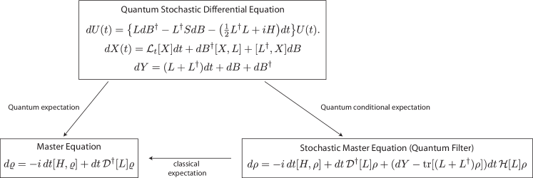
Figure 3: Relationship between QSDEs for the unitary, system and environment; master equation; and stochastic master equation (filter) for open quantum systems (${\mathcal{H}}_{L}$ is given by (14). The difference between the master equation and stochastic master equation is due to the difference in the type of expectation take, i.e. unconditioned or conditioned, respectively.

Now let us return to the vacuum state for the field: $\rho_{\text{field}}=P_{\text{vac}}$. We shall recall a simple derivation of the filter using an analogue of a the characteristic function technique of classical filtering AM . We introducing a process $C\left(t\right)$ satisfying the QSDE

$$dC\left(t\right)=g\left(t\right)C\left(t\right)dY\left(t\right),$$ (10)

with initial condition $C\left(0\right)=I$. Here we assume that $g$ is integrable, but otherwise arbitrary. The technique is to make an ansatz of the form

$$d\pi_{t}\left(X\right)=\alpha_{t}dt+\beta_{t}\left(X\right)dY\left(t\right)$$ (11)

where we assume that the processes $\alpha_{t}$ and $\beta_{t}$ are adapted and lie in $\mathcal{Y}_{t}$. These coefficients may be deduced from the identity

$$\mathbb{E}\left[\left(\pi_{t}\left(X\right)-j_{t}\left(X\right)\right)C\left(t\right)\right]=0$$

which is valid since $C(t)$ is in $\mathcal{Y}_{t}$. We note that the Itō product rule implies $I+II+III=0$ where

$$I = \mathbb{E}\left[\left(d\pi_{t}\left(X\right)-dj_{t}\left(X\right)\right)C\left(t\right)\right],$$

$$= \mathbb{E}\left[\alpha_{t}C\left(t\right)+\beta_{t}j_{t}\left(L+L^{{\dagger}}\right)C\left(t\right)\right]dt$$

$$-\mathbb{E}\left[j_{t}\left(\mathcal{L}_{G}X\right)C\left(t\right)\right]dt,$$

$$II = \mathbb{E}\left[\left(\pi_{t}\left(X\right)-j_{t}\left(X\right)\right)dC\left(t\right)\right],$$

$$= \mathbb{E}\left[\left(\pi_{t}\left(X\right)-j_{t}(X)\right)g\left(t\right)C\left(t\right)j_{t}\left(L+L^{{\dagger}}\right)\right]dt,$$

$$III = \mathbb{E}\left[\left(d\pi_{t}\left(X\right)-dj_{t}\left(X\right)\right)dC\left(t\right)\right]$$

$$= \mathbb{E}\left[\beta_{t}g\left(t\right)C\left(t\right)\right]dt+\mathbb{E}\left[g(t)j_{t}([L^{\dagger},X])C(t)\right]dt.$$

Now from the identity $I+II+III=0$ we may extract separately the coefficients of $g\left(t\right)C\left(t\right)$ and $C\left(t\right)$ as $g\left(t\right)$ was arbitrary to deduce

$$\pi_{t}\left(\left(\pi_{t}\left(X\right)-j_{t}(X)\right)j_{t}\left(L+L^{{\dagger}}\right)\right)+\pi_{t}\left(\beta_{t}\right) = 0,$$

$$\pi_{t}\left(\alpha_{t}+\beta_{t}j_{t}\left(L+L^{{\dagger}}\right)-j_{t}\left(\mathcal{L}_{G}X\right)\right) = 0.$$

Using the projective property of the conditional expectation $\pi_{t}((\pi_{t}X))=\pi_{t}(X)$ and the assumption that $\alpha_{t}$ and $\beta_{t}$ lie in $\mathcal{Y}_{t}$, we find after a little algebra that

$$\beta_{t} = \pi_{t}\left(XL+L^{{\dagger}}X\right)-\pi_{t}\left(X\right)\pi_{t}\left(L+L^{{\dagger}}\right),$$

$$\alpha_{t} = \pi_{t}\left(\mathcal{L}_{G}X\right)-\beta_{t}\pi_{t}\left(L+L^{{\dagger}}\right),$$

so that the equation (11) reads as

$$d\pi_{t}(X) = \pi_{t}(\mathcal{L}_{G}X)dt$$

$$+(\pi_{t}(XL+L^{{\dagger}}X)-\pi_{t}(L+L^{{\dagger}})\pi_{t}(X))dW(t),$$

where the innovations process $W(t)$ is a Wiener process. It is related to the measurement process $Y(t)$ by the equation

$$dY(t)=\pi_{t}(L+L^{{\dagger}})dt+dW(t)$$ (13)

and has the interpretation as given the difference between the observed change $dY(t)$ and the expected change $\pi_{t}(L+L^{{\dagger}})dt$ in the measured field immediately after time $t$. Note that the increment $dW(t)$ of the innovations process is independent of $\pi_{s}(X)$ for all $0\leq s\leq t$.

It important to note that $Q(t)$ (equivalent to a Wiener process) and $W(t)$ (also a Wiener process) are distinct, and that $Q(t)$ is not in the commutative observation subspace. Some care is needed in interpreting equation (II.5) for the quantum filter. All of the terms in this equation belong to the commutative subspace $\mathcal{Y}_{t}$, and so (by the spectral theorem BouvanHJam07 ) are statistically equivalent to classical stochastic processes.

The stochastic master equation may be expressed in terms of the density operator-valued stochastic process $\rho(t)$:

$$d\rho(t)=\mathcal{L}_{G}^{\star}\rho(t)dt+\mathcal{H}_{L}\rho(t)\,dW(t).$$

where we introduce

$$\mathcal{H}_{L}\rho=L\rho+L^{{\dagger}}\rho-\mathrm{tr}\left\{\left(L+L^{{\dagger}}\right)\rho\right\}\,\rho.$$ (14)

The increments $dW(t)$ can be generated independently of $\rho(s)$ for all $0\leq s\leq t$ and the stochastic master equation above driven by the generated increments can thus act as a simulated quantum trajectory of the state conditioned upon the measurement outcomes $\{y(s);\;0\leq s\leq t\}$.

II.6 Photon Counting Case

If instead we measure the number observable $Y(t)=U^{{\dagger}}(t)\Lambda(t)U(t)=\Lambda_{out}(t)=\int_{0}^{t}b_{out}^{{\dagger}}(s)b_{out}(s)ds$ then the quantum filter is (see the survey paper BouvanHJam07 for the derivation),

$$d\rho(t)=\mathcal{L}_{G}^{\star}\rho(t)dt+\mathcal{J}_{L}\rho(t)\,dN(t)$$

where

$$\mathcal{J}_{L}\rho=\frac{L\rho L^{{\dagger}}}{\mathrm{tr}\left\{\rho L^{{\dagger}}L\right\}}-\rho,$$

and the innovations process in this case is given by $dN(t)=dY-\mathrm{tr}\{\rho(t)L^{{\dagger}}L\}dt$ and is a compensated Poisson process of intensity $\mathrm{tr}\{\rho(t)L^{{\dagger}}L\}$.

II.7 Cascade Connections

A simple quantum network may be formed by connecting the output of one system to the input of another system, Gar93 ; Car93 ; YanKim03_1 ; GouJam09b . Fig. 4 illustrates the open quantum system $G=(S,L,H)$ equivalent to the cascade of systems $G_{1}=(S_{1},L_{1},H_{1})$ and $G_{2}=(S_{2},L_{2},H_{2})$. This equivalent system can be described in terms of the series product $G_{T}=G_{2}\triangleleft G_{1}$ GouJam09b , defined by

$$G_{2}\triangleleft G_{1}=(S_{2}S_{1},L_{2}+S_{2}L_{1},H_{1}+H_{2}+\mathrm{Im}\{L_{2}^{\dagger}S_{2}L_{1}]\}).$$ (15)

Note in equation (15) the order of the operators is important. The series product provides the three parameters for the combined or total open system $G$ in terms of the parameters for each of the systems $G_{1}$ and $G_{2}$.

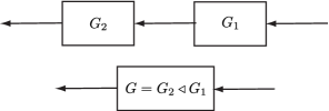
Figure 4: Two quantum systems cascaded, so that the output of system $G_{1}$ becomes the input of system $G_{2}$. Importantly the flow of information is directional. In (b) the circuit has been simplified using quantum network theory to an equivalent system $G=G_{2}\triangleleft G_{1}$. This type of network topology is called a cascade or series connection.

III Single Photon Fields

The master equation for a Markovian coupling of a system to a boson field in a continuous-mode one or two photon state was first treated in  GheEllPelZol99 . In this section, we review the problem of determining the associated filter (stochastic master equation) for an arbitrary system $G=(S,L,H)$ driven by a single photon field GJN11a . In section III.7 we generalize the master equation and filter to include any combination of single photon and vacuum as a probe field. The final section, section III.8, is an explicit example of the homodyne single photon filtering equations for a two level atom.

III.1 Continuous-Mode Single Photon States

There are many ways to generate single photon states single-photon-production . One common technique for creating heralded single photon states is by spontaneous parametric downconversion (SPDC). The photons from such a process are inherently multimodal SPDC-mulitmode , and spectral filtering is typically performed to get a single mode photon.

The creation operator for a photon with one-particle state $\xi$ is

$$B^{{\dagger}}\left(\xi\right)=\int_{0}^{\infty}\xi\left(t\right)dB^{{\dagger}}\left(t\right)$$ (16)

normalized so that $\left\|\xi\right\|^{2}=\int_{0}^{\infty}\left|\xi\left(t\right)\right|^{2}dt=1$. The single photon state is then defined to be

$$|1_{\xi}\rangle=B^{{\dagger}}(\xi)|0\rangle.$$ (17)

One may interpret this is the frequency domain as $|1_{\xi}\rangle=\int_{-\infty}^{\infty}\hat{\xi}(\omega)\hat{b}^{{\dagger}}(\omega)|0\rangle$ where $\hat{\xi}$ is the Fourier transform of  $\xi$ and $\hat{b}\left(\omega\right)$ the formal transform of the input process. This representation is often referred to as the multimode, or continuous-mode, single photon state, see for instance (Lou_book00, , Sec. 6.3), (Mil07, , Sec. 14.2), (Mil08, , Eq. (9)).

Much of the calculations that follow will involve the identities

$$dB(t)|1_{\xi}\rangle = \xi(t)|0\rangle dt,$$

$$d\Lambda(t)|1_{\xi}\rangle = \xi(t)dB^{{\dagger}}(t)|0\rangle,$$ (18)

and this will be the origin of the departure of the master and filter equations from the vacuum case.

III.2 Single Photon Master Equation

Without loss of generality we fix the initial state of the system to be a pure state $\rho_{0}=|\eta\rangle\langle\eta|$ and our aim is to obtain a differential equation for the expectation

$$\varpi_{t}^{11}\left(X\right)=\langle\eta 1_{\xi}|j_{t}\left(X\right)|\eta 1_{\xi}\rangle,$$

for arbitrary system operator $X$. Starting from the Heisenberg-Langevin equation as before, but now using the identities (18) we find

$$\frac{d}{dt}\varpi_{t}^{11}\left(X\right)=\mathbb{E}_{11}[j_{t}(\mathcal{L}_{G}X))]\\ +\mathbb{E}_{01}[j_{t}(S^{{\dagger}}[X,L])]\,\xi^{\ast}(t)+\mathbb{E}_{10}[j_{t}([L^{{\dagger}},X]S)]\,\xi(t)\\ +\mathbb{E}_{00}[j_{t}(S^{{\dagger}}XS-X)]\,|\xi(t)|^{2}\\ =\varpi_{t}^{11}(\mathcal{L}_{G}X)+\varpi_{t}^{01}(S^{{\dagger}}[X,L])\,\xi^{\ast}(t)\\ +\varpi_{t}^{10}([L^{{\dagger}},X]S)\,\xi(t)+\varpi_{t}^{00}(S^{{\dagger}}XS-X)\,|\xi(t)|^{2}$$

where

$$\mathbb{E}_{jk}\left[A\right] = \langle\eta\phi_{j}|A|\eta\phi_{k}\rangle$$

$$\varpi_{t}^{jk}\left(X\right) = \mathbb{E}_{jk}[j_{t}\left(X\right)]$$

with

$$\phi_{j}=\left|\begin{array}[]{cc}|0\rangle,&j=0;\\ |1_{\xi}\rangle,&j=1.\end{array}\right\}$$

Rather than finding a single master equation as in the vacuum case, we end up with a system of equations

$$\dot{\varpi}_{t}^{11}(X) =\varpi_{t}^{11}(\mathcal{L}X)+\varpi_{t}^{01}(S^{{\dagger}}[X,L])\xi^{\ast}(t)$$

$$+ \varpi_{t}^{10}([L^{{\dagger}},X]S)\xi(t)+\varpi_{t}^{00}(S^{{\dagger}}XS-X)|\xi(t)|^{2},$$

$$\dot{\varpi}_{t}^{10}(X) =\varpi_{t}^{10}(\mathcal{L}X)+\varpi_{t}^{00}(S^{{\dagger}}[X,L])\xi^{\ast}\!(t),$$

$$\dot{\varpi}_{t}^{01}(X) =\varpi_{t}^{01}(\mathcal{L}X)+\varpi_{t}^{00}([L^{{\dagger}},X]S)\xi(t),$$

$$\dot{\varpi}_{t}^{00}(X) =\varpi_{t}^{00}(\mathcal{L}X),$$ (19)

with initial conditions

$$\varpi_{0}^{11}(X)=\varpi_{0}^{00}(X)=\langle\eta,X\eta\rangle,\ \ \varpi_{0}^{10}(X)=\varpi_{0}^{01}(X)=0.$$ (20)

The main feature here is that the differential equation for expectations $\varpi^{jk}$ depends on lower order $\varpi^{jk}$, allowing us to solve for $\varpi^{11}$ inductively. Likewise, defining the traceclass operators $\varrho^{jk}$ via

$$\mathrm{tr}\left\{\varrho^{jk}(t)^{{\dagger}}X\right\}=\varpi_{t}^{jk}(X),$$ (21)

we obtain a system of equations

$$\dot{\varrho}^{11}(t) =\mathcal{L}^{\star}\varrho^{11}(t)+\![S\rho^{01}(t),L^{{\dagger}}]\xi(t)+\![L,\varrho^{10}(t)S^{{\dagger}}]\xi^{\ast}\!(t)$$

$$+(S\rho^{00}(t)S^{{\dagger}}-\varrho^{00}(t))|\xi(t)|^{2},$$

$$\dot{\varrho}^{10}(t) =\mathcal{L}^{\star}\varrho^{10}(t)+[S\rho^{00}(t),L^{{\dagger}}]\xi(t),$$

$$\dot{\varrho}^{01}(t) =\mathcal{L}^{\star}\varrho^{01}(t)+[L,\varrho^{00}(t)S^{{\dagger}}]\xi^{\ast}(t),$$

$$\dot{\varrho}^{00}(t) =\mathcal{L}^{\star}\varrho^{00}(t),$$ (22)

with

$$\varrho^{11}(0)=\varrho^{00}(0)=|\eta\rangle\langle\eta|,\ \ \varrho^{10}(0)=\varrho^{01}(0)=0.$$

Note $\varrho^{jk}(t)^{{\dagger}}=\varrho^{kj}(t)$.

III.3 An Input-Output Model of Single Photon Signal Generation

In section III.5 we will set up a general technique for deriving the filtering equations for situations including the single photon input field. It is possible to give an alternate derivation in this case motivated by the idea of using a pre-interaction preparation where a vacuum input is first passed through a fixed system in order to generate the one photon field. Our motivation for considering such a scenario stems from statistical and engineering modelling where it is common practice to use ‘signal generating filters’ AM driven by white noise to represent colored noise. Analogously, in this section, we construct a quantum signal generating filter $M=(S_{M},L_{M},H_{M})$. Cascading the single photon generating filter $M$ with the quantum system $G$ we wish to probe, Figure 5, we create an extended system. Because this extended system $G_{T}=G\triangleleft M$ is driven by vacuum, the master equation and quantum filter follow from the known vacuum case upon substitution of the parameters for the cascade system (Section III.5). We stress that the signal generation model here (and in Section IV.3 for the case of a system driven by a superposition of continuous-mode coherent states) serves only as a convenient theoretical mathematical device to derive the quantum filtering (or stochastic master) equations. It is not suggested that single photons with a given wavepacket shape are to be generated in practice with physical devices that implement this particular generator.

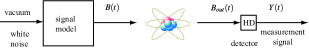
Figure 5: An ancilla system $M$ is used to model the effect of the single photon state for $B(t)$ on the system $G$.

The idea behind the signal generating filter $M$ is simple. We take the filter to be a two level atom initially prepared in its excited state $|\uparrow\rangle$. The interaction with the vacuum input is taken to be

$$(S_{M},L_{M},H_{M})=\left(I,\lambda\left(t\right)\sigma_{-},0\right),$$ (23)

which means that at some stage the atom decays into its ground state $|\downarrow\rangle$ creating a single photon in the output. The mechanism for producing the single photon is therefore spontaneous emission due to the coupling to the vacuum fluctuations. Here $\sigma_{-}$ is the lowering operator from the upper state $|\uparrow\rangle$ to the ground state $|\downarrow\rangle$. The Schrödinger equation for $|\psi_{t}\rangle=V(t)|\uparrow\rangle\otimes|0\rangle$ then becomes $d|\psi_{t}\rangle=\left[\lambda\left(t\right)\sigma_{-}dB_{t}^{\ast}-\frac{1}{2}\left|\lambda\left(t\right)\right|^{2}\sigma_{+}\sigma_{-}dt\right]\,|\psi_{t}\rangle$, and it is an elementary calculation to see that this has the exact solution

$$|\psi_{t}\rangle=\sqrt{w\left(t\right)}|\uparrow\rangle\otimes|0\rangle+|\downarrow\rangle\otimes B_{t}^{\ast}(\xi)|0\rangle$$ (24)

where $B_{t}^{\ast}\left(\xi\right)=\int_{0}^{t}\xi_{s}dB_{s}^{\ast}$, and (to preserve normalization) $w\left(t\right)=\int_{t}^{\infty}\left|\xi\left(s\right)\right|^{2}ds$ with the complex-valued function $\xi\left(\cdot\right)$ related to $\lambda\left(\cdot\right)$ by

$$\lambda\left(t\right)=\frac{1}{\sqrt{w\left(t\right)}}\xi\left(t\right).$$ (25)

Since $w\left(0\right)=\left\|\xi\right\|^{2}=1$, we therefore generate the limit state

$$|\psi_{\infty}\rangle=|\downarrow\rangle\otimes B^{{\dagger}}\left(\xi\right)|0\rangle\equiv|\downarrow\rangle\otimes|1_{\xi}\rangle.$$

Thus the generator model will output the desired single photon state $|1_{\xi}\rangle$ provided that we choose the (time-dependent) coupling strength $\lambda(t)$ according to (25).

III.4 The Extended System

We now define our extended system as the cascade system $G_{T}=G\triangleleft M$, as in Figure 5, where using the cascade connection formalism from Section II.7 we have

$$G_{T} =G\triangleleft M$$

$$=\left(S,L+\frac{\xi(t)}{\sqrt{w(t)}}S\sigma_{-},H+\frac{\xi(t)}{\sqrt{w(t)}}\mathrm{Im}(L^{{\dagger}}S\sigma_{-})\right).$$ (26)

Let us denote by $\tilde{U}(t)$ the unitary for the extended system driven by vacuum for the parameters $G_{T}$ on the ancilla+system Hilbert space. Specifying an initial state $|\uparrow\rangle\otimes|\eta\rangle\otimes|0\rangle$, we consider the expectation

$$\tilde{\varpi}_{t}(A\otimes X)=\mathbb{E}_{\uparrow\eta 0}[\tilde{U}^{\dagger}(t)(A\otimes X)\tilde{U}(t)],$$ (27)

(here $A$ is an ancilla operator, and $X$ is a system operator).

In order to be useful, the extended system $G_{T}$ (driven by vacuum) must be capable of capturing expectations of $X(t)$, for arbitrary operator $X$ of the system $G$, at time $t$ as if it were driven by the single photon field. That is, we must have

$$\mathbb{E}_{\eta\xi}[X(t)]=\mathbb{E}_{\uparrow\eta 0}[\tilde{U}^{{\dagger}}(t)(I\otimes X\otimes I)\tilde{U}(t)],$$ (28)

that is we have the situation outlined in equation (1) with

$$\rho_{a}=|\uparrow\rangle\langle\uparrow|,\quad R(t)=I.$$

We are required to show that

$$\mathbb{E}_{\eta\xi}[X(t)]=\mathbb{E}_{\uparrow\eta 0}[\tilde{U}^{{\dagger}}(t)(I\otimes X)\tilde{U}(t)]$$ (29)

holds for any operator $X$ of the system $G$.

Our verification of (29) is to compare the differentials of both sides. Now the left hand side of (29) is just the single photon expectation $\varpi_{t}^{11}(X)=\mathbb{E}_{11}[X(t)]=\mathbb{E}_{\eta\xi}[X(t)]$, whose differential equation is determined from the system (19). The differential of the right hand side of (29) may be found using the Lindblad superoperator $\mathcal{L}_{G_{T}}[A\otimes X]\!$ for the extended system, which may be expressed in the form

$$\mathcal{L}_{G_{T}}[A\otimes X]\! =A\otimes\mathcal{L}_{G}X+(\mathcal{D}_{L_{M}}A)\otimes X$$

$$+L_{M}^{{\dagger}}A\otimes S^{{\dagger}}[X,L]+AL_{M}\otimes[L^{{\dagger}},X]S$$

$$+L_{M}^{{\dagger}}AL_{M}\otimes(S^{{\dagger}}XS-X),$$

for any ancilla operator $A$ and system operator $X$. We first observe that

$$\mathcal{D}_{L_{M}}(I)=0,\ \ \mathcal{D}_{L_{M}}(\sigma_{-})=-\frac{|\xi(t)|^{2}}{2w(t)}\sigma_{-},$$

$$\mathcal{D}_{L_{M}}(\sigma_{+})=-\frac{|\xi(t)|^{2}}{2w(t)}\sigma_{+},\ \ \mathcal{D}_{L_{M}}(\sigma_{+}\sigma_{-})=-\frac{|\xi(t)|^{2}}{w(t)}\sigma_{+}\sigma_{-},$$

where $w(t)=\int_{t}^{\infty}|\xi(s)|^{2}ds$. Then we have

$$\frac{d}{dt}\mathbb{E}_{\uparrow\eta 0}[\tilde{U}^{{\dagger}}(t)(I\otimes X)\tilde{U}(t)]=$$

$$\tilde{\varpi}_{t}^{11}(\mathcal{L}_{G}X)+\tilde{\varpi}_{t}^{01}(S^{{\dagger}}[X,L])\xi^{\ast}(t)$$

$$+\tilde{\varpi}_{t}^{10}([L^{{\dagger}},X]S)\xi(t)+\tilde{\varpi}_{t}^{00}(S^{{\dagger}}XS-X)|\xi(t)|^{2},$$ (30)

where

$$\tilde{\varpi}_{t}^{jk}(X)=\frac{\tilde{\varpi}_{t}(Q_{jk}\otimes X)}{w_{jk}(t)},$$ (31)

with

$$\left(Q_{jk}\right) = \left(\begin{array}[]{cc}Q_{00}&Q_{01}\\ Q_{10}&Q_{11}\end{array}\right)=\left(\begin{array}[]{cc}\sigma_{+}\sigma_{-}&\sigma_{+}\\ \sigma_{-}&I\end{array}\right),$$

$$\left(w_{jk}\right) = \left(\begin{array}[]{cc}w_{00}&w_{01}\\ w_{10}&w_{11}\end{array}\right)=\left(\begin{array}[]{cc}w(t)&\sqrt{w(t)}\\ \sqrt{w(t)}&1\end{array}\right).$$

Notice that equation (30) for $\tilde{\varpi}_{t}^{11}(X)$ has the same form as the $\varpi_{t}^{11}(X)$ equation in (19). In general, the equations for $\tilde{\varpi}_{t}^{jk}(X)$ have the same form as equations (19) for $\varpi_{t}^{jk}(X)$. Since at time $t=0$ we have $\tilde{\varpi}_{0}^{jk}(X)=\varpi_{0}^{jk}(X)$, it follows that $\tilde{\varpi}_{t}^{jk}(X)=\varpi_{t}^{jk}(X)$ for all $t$. This establishes the identity (29).

III.5 Single Photon Stochastic Master Equation (Filter) for Quadrature Phase Measurements

In this section we explain how the quantum filter for the conditional expectation

$$\pi_{t}^{11}(X)=\mathbb{E}_{\eta\xi}[X(t)|Y(s),0\leq s\leq t]$$

for the system $G$ driven by a single photon field may now be obtained from the quantum filter for the conditional expectation

$$\tilde{\pi}_{t}(A\otimes X)=\mathbb{E}_{\uparrow\eta 0}[\tilde{U}^{\dagger}(t)(A\otimes X)\tilde{U}(t)|I\otimes Y(s),0\leq s\leq t]$$ (34)

for the extended system $G_{T}=G\triangleleft M$ driven by vacuum.

Indeed, we have

$$d\tilde{\pi}_{t}(A\otimes X) = \tilde{\pi}_{t}(\mathcal{L}_{G_{T}}(A\otimes X))dt$$ (35)

$$+(\tilde{\pi}_{t}(A\otimes XL_{T}+L_{T}^{\dagger}A\otimes X)$$

$$-\tilde{\pi}_{t}(L_{T}+L_{T}^{\dagger})\tilde{\pi}_{t}(A\otimes X))dW(t),$$

where $dW(t)=dY(t)-\tilde{\pi}_{t}(L_{T}+L_{T}^{\dagger})dt$. If we define

$$\pi^{jk}_{t}(X)=\frac{\tilde{\pi}_{t}(Q_{jk}\otimes X)}{w_{jk}(t)},$$ (36)

where $Q_{jk}$ and $w_{jk}(t)$ were defined in the previous section, we obtain the coupled system of nonlinear stochastic differential equations

$$d\pi^{11}_{t}(X)= \bigl{\{}\pi^{11}_{t}(\mathcal{L}X)+\pi^{01}_{t}(S^{\dagger}[X,L])\xi^{\ast}(t)+\pi^{10}_{t}([L^{\dagger},X]S)\xi(t)+\pi^{00}_{t}(S^{\dagger}XS-X)|\xi(t)|^{2}\bigr{\}}dt$$

$$+\big{\{}\pi^{11}_{t}(XL+L^{\dagger}X)+\pi^{01}_{t}(S^{\dagger}X)\xi^{\ast}(t)+\pi^{10}_{t}(XS)\xi(t)-\pi^{11}_{t}(X)K_{t}\big{\}}dW(t),$$

$$d\pi^{10}_{t}(X)= \bigl{\{}\pi^{10}_{t}(\mathcal{L}X)+\pi^{00}_{t}(S^{\dagger}[X,L])\xi^{\ast}(t)\bigr{\}}dt+\big{\{}(\pi^{10}_{t}(XL+L^{\dagger}X)+\pi^{00}_{t}(S^{\dagger}X)\xi^{\ast}(t)-\pi^{10}_{t}(X)K_{t}\big{\}}dW(t),$$

$$d\pi^{01}_{t}(X)= \bigl{\{}\pi^{01}_{t}(\mathcal{L}X)+\pi^{00}_{t}(S^{\dagger}[X,L])\xi^{\ast}(t)\bigr{\}}dt+\big{\{}(\pi^{01}_{t}(XL+L^{\dagger}X)+\pi^{00}_{t}(S^{\dagger}X)\xi^{\ast}(t)-\pi^{01}_{t}(X)K_{t}\big{\}}dW(t),$$

$$d\pi^{00}_{t}(X)= \pi^{00}_{t}(\mathcal{L}X)dt+\big{\{}\pi^{00}_{t}(XL+L^{\dagger}X)-\pi^{00}_{t}(X)K_{t}\big{\}}dW(t).$$ (37)

Here,

$$K_{t}=\pi^{11}_{t}(L+L^{\dagger})+\pi^{01}_{t}(S)\xi(t)+\pi^{10}_{t}(S^{\dagger})\xi^{\ast}(t)$$ (38)

and the innovations process $W(t)$ (given above) may be expressed as

$$dW(t)=dY(t)-K_{t}dt.$$ (39)

We have $\pi^{01}_{t}(X)=\pi^{10}_{t}(X^{\dagger})^{\dagger}$, and the initial conditions are $\pi^{11}_{0}(X)=\pi^{00}_{0}(X)=\langle\eta,X\eta\rangle,\ \ \pi^{10}_{0}(X)=\pi^{01}_{0}(X)=0.$

In order to see that the single photon quantum filter is given by the system of coupled equations (37), we must show that the conditional expectation for the system driven by the single photon field is given by

$$\pi_{t}(X) = \mathbb{E}_{\eta\xi}[X(t)|Y(s),\ 0\leq s\leq t]$$ (40)

$$= \mathbb{E}_{\uparrow\eta 0}[\tilde{U}^{{\dagger}}(t)(A\otimes X)\tilde{U}(t)|I\otimes Y(s),0\leq s\leq t]$$

$$= \pi_{t}^{11}(X).$$

To obtain the filter, we again apply the characteristic function technique, setting $C=C_{g}(t)$ as before with $dc_{g}(t)=g(t)c_{g}(t)dY(t)$. We need to verify that

$$\mathbb{E}_{\eta 0}[j_{t}(X)c_{g}(t)]=\mathbb{E}_{\eta 0}[\pi_{t}(X)c_{g}(t)]$$ (41)

For the extended system we have

$$\mathbb{E}_{\uparrow\eta 0}[\tilde{U}^{{\dagger}}(t)(A\otimes X)\tilde{U}(t)c_{g}(t)]=\mathbb{E}_{\eta 0}[\tilde{\pi}_{t}(A\otimes X)c_{g}(t)],$$ (42)

for all functions $g$, arbitrary ancilla, and system operators $A$ and $X$ respectively. Hence (41) will follow provided we can show that

$$\mathbb{E}_{jk}[X(t)c_{g}(t)]=\frac{\mathbb{E}_{e\eta 0}[\tilde{U}^{{\dagger}}(t)(Q_{jk}\otimes X)\tilde{U}(t)c_{g}(t)]}{w_{jk}(t)}.$$ (43)

However, equation (43) may be verified in exactly the same way we proved that $\tilde{\varpi}_{t}^{jk}(X)=\varpi_{t}^{jk}(X)$ in the previous section, that is, by comparing the differentials of both sides of (43). The details of this calculation are omitted.

Now, write $\pi_{t}^{jk}(X)=\mathrm{tr}(($$\varrho$${}^{jk}(t))^{{\dagger}}X)$. Then from the differential equations for $\pi_{t}^{jk}(X)$ and the definition $\varrho$${}^{jk}(t)$ we immediate get the differential equations for the evolution of $\varrho$${}^{jk}(t)$, as follows:

$$d\rho^{11}(t) = \bigl{\{}\mathcal{L}^{\star}\rho^{11}(t)+[S\rho^{01}(t),L^{\dagger}]\xi(t)+[L,\rho^{10}(t)S^{\dagger}]\xi^{\ast}(t)+(S\rho^{00}(t)S^{\dagger}-\rho^{00}(t))|\xi(t)|^{2}\big{\}}dt$$

$$+\big{\{}L\rho^{11}(t)+\rho^{11}(t)L^{\dagger}+\rho^{10}(t)S^{\dagger}\xi^{\ast}(t)+S\rho^{01}(t)\xi(t)-K_{t}\rho^{11}(t)\big{\}}dW(t),$$

$$d\rho^{10}(t) = \big{\{}\mathcal{L}^{\star}\rho^{10}(t)+[S\rho^{00}(t),L^{\dagger}]\xi(t)\big{\}}dt+\big{\{}L\rho^{10}(t)+\rho^{10}(t)L^{\dagger}+S\rho^{00}(t)\xi(t)-K_{t}\rho^{10}(t)\big{\}}dW(t),$$

$$d\rho^{01}(t) = \big{\{}\mathcal{L}^{\star}\rho^{01}(t)+[L,\rho^{00}(t)S^{\dagger}]\xi^{\ast}(t)\big{\}}dt+\big{\{}L\rho^{01}(t)+\rho^{01}(t)L^{\dagger}+\rho^{00}(t)S^{\dagger}\xi^{\ast}(t)-K_{t}\rho^{01}(t)\big{\}}dW(t),$$

$$d\rho^{00}(t) = \mathcal{L}^{\star}\rho^{00}(t)dt+\big{\{}L\rho^{00}(t)+\rho^{00}(t)L^{\dagger}-K_{t}\rho^{00}(t)\big{\}}dW(t),$$ (44)

where

$$K_{t} \equiv\mathrm{tr}\{{{(L+L^{{\dagger}})\rho^{11}(t)\}}}$$

$$+\mathrm{tr}\{S\rho{{{}^{01}(t)\}}}\xi(t)+\mathrm{tr}\{{{S^{{\dagger}}\rho^{10}(t)\}}}\xi^{\ast}(t),$$

with the initial condition

$$\rho^{11}(0) =\rho^{00}(0)=|\eta\rangle\langle\eta|,\;\rho^{10}(0)=\rho^{01}(0)=0.$$

III.6 Single Photon Stochastic Master Equation (Filter) for Photon Counting Measurements

In this section we briefly derive the filtering equations for photon counting measurements. The quantum filter for the photon counting case is given by the system of equations

$$d\pi^{11}_{t}(X) = \{\pi^{11}_{t}(\mathcal{L}X)+\pi^{01}_{t}(S^{\dagger}[X,L])\xi^{\ast}(t)+\pi^{10}_{t}([L^{\dagger},X]S)\xi(t)+\pi^{00}_{t}(S^{\dagger}XS-X)|\xi(t)|^{2}\}dt$$

$$+\biggl{\{}\nu_{t}^{-1}\left(\pi^{11}_{t}(L^{\dagger}XL)+\pi^{01}_{t}(S^{\dagger}XL)\xi^{\ast}(t)+\pi^{10}_{t}(L^{\dagger}XS)\xi(t)+\pi^{00}_{t}(S^{\dagger}XS)|\xi(t)|^{2}\right)-\pi^{11}_{t}(X)\biggr{\}}dN(t),$$

$${d\pi^{10}_{t}(X)} = \{\pi^{10}_{t}(\mathcal{L}X)+\pi^{00}_{t}(S^{\dagger}[X,L])\xi^{\ast}(t)\}dt+\biggl{\{}\nu_{t}^{-1}\left(\pi^{10}_{t}(L^{\dagger}XL)+\pi^{00}_{t}(S^{\dagger}XL)\xi^{\ast}(t)\right)-\pi^{10}_{t}(X)\biggr{\}}dN(t),$$

$$d\pi^{01}_{t}(X) = \{\pi^{01}_{t}(\mathcal{L}X)+\pi^{00}_{t}([L^{\dagger},X]S)\xi(t)\}dt+\bigg{\{}\nu_{t}^{-1}\left(\pi^{01}_{t}(L^{\dagger}XL)+\pi^{00}_{t}(L^{\dagger}XS)\xi(t)\right)-\pi^{01}_{t}(X)\bigg{\}}dN(t),$$

$$d\pi^{00}_{t}(X) = \pi^{00}_{t}(\mathcal{L}X)dt+\biggl{\{}\nu_{t}^{-1}\bigl{(}\pi^{00}_{t}(L^{\dagger}XL)\bigr{)}-\pi^{01}_{t}(X)\biggr{\}}dN(t),$$

or in the Schrödinger-picture

$$d\rho^{11}(t) = \bigl{\{}\mathcal{L}^{\star}\rho^{11}(t)+[S\rho^{01}(t),L^{\dagger}]\xi(t)+[L,\rho^{10}(t)S^{\dagger}]\xi^{\ast}(t)+(S\rho^{00}(t)S^{\dagger}-\rho^{00}(t))|\xi(t)|^{2}\big{\}}dt$$

$$+\biggl{\{}\nu_{t}^{-1}\left(L\rho^{11}(t)L^{\dagger}+L\rho^{10}(t)S^{\dagger}\xi^{\ast}(t)+S\rho^{10}(t)L^{\dagger}\xi(t)+S\rho^{00}(t)S^{\dagger}|\xi(t)|^{2}\right)-\rho^{11}(t)\biggr{\}}dN(t),$$

$$d\rho^{10}(t) = \big{\{}\mathcal{L}^{\star}\rho^{10}(t)+[S\rho^{00}(t),L^{\dagger}]\xi(t)\big{\}}dt+\biggl{\{}\nu_{t}^{-1}\left(L\rho^{10}(t)L^{\dagger}+S\rho^{00}(t)L^{\dagger}\xi(t)\right)-\rho^{10}(t)\biggr{\}}dN(t),$$

$$d\rho^{01}(t) = \big{\{}\mathcal{L}^{\star}\rho^{01}(t)+[L,\rho^{00}(t)S^{\dagger}]\xi^{*}\!(t)\big{\}}dt+\bigg{\{}\nu_{t}^{-1}\left(L\rho^{01}(t)L^{\dagger}+L\rho^{00}(t)S^{\dagger}\xi^{*}(t)\right)-\rho^{01}(t)\bigg{\}}dN(t),$$

$$d\rho^{00}(t) = \mathcal{L}^{\star}\rho^{00}(t)dt+\biggl{\{}\nu_{t}^{-1}\bigl{(}L\rho^{00}(t)L^{\dagger}\bigr{)}-\rho^{00}(t)\biggr{\}}dN(t),$$ (45)

where

$$\nu_{t} =\pi^{11}_{t}(L^{\dagger}L)+\pi^{01}_{t}(S^{\dagger}L)\xi^{\ast}(t)$$

$$+\pi^{10}_{t}(L^{\dagger}S)\xi(t)+\pi^{00}_{t}(I)|\xi(t)|^{2},$$

$$={\rm Tr}\left[{{\rho^{11}(t)L^{\dagger}L}}\right]+{\rm Tr}\left[{{\rho^{10}(t)S^{\dagger}L}}\right]\xi^{\ast}(t)$$

$$+{\rm Tr}\left[{{\rho^{01}(t)L^{\dagger}S}}\right]\xi(t)+{\rm Tr}\left[{{\rho^{00}(t)I}}\right]|\xi(t)|^{2},$$

and the innovations process $N(t)$ is given by

$$dN(t)=dY(t)-\nu_{t}dt.$$

III.7 Combination of One Photon and Vacuum States

In this section we take the state of the field to be in a state defined by the density operator

$$\rho_{\mathrm{field}}=\sum_{jk}\gamma_{kj}|\phi_{j}\rangle\langle\phi_{k}|$$ (46)

where we use the notation introduced above for the photon $|\phi_{1}\rangle=|1_{\xi}\rangle$ and vacuum $|\phi_{0}\rangle=|0\rangle$ states. The coefficients $\gamma_{jk}$ must of course satisfy the condition that the $2\times 2$ complex matrix

$$\rho_{a}=\sum_{jk}\gamma_{kj}|j\rangle\langle k|=\left(\begin{array}[]{cc}\gamma_{11}&\gamma_{10}\\ \gamma_{01}&\gamma_{00}\end{array}\right)$$ (47)

is a density matrix, i.e. $\rho_{a}\geq 0$, $\mathrm{Tr}[\rho_{a}]=1$. By choosing the coefficients $\gamma_{jk}$ appropriately we can model an input field that is any combination of single photon and vacuum. For example: the single photon field is given by $\gamma_{11}=1$ and all other coefficients are zero, a superposition like $\left|{\psi}\right\rangle_{f}=\alpha_{1}\left|{1_{\xi}}\right\rangle+\alpha_{0}\left|{0}\right\rangle$ is obtained by setting $\gamma_{11}=|\alpha_{1}|^{2},\,\gamma_{10}=\alpha_{1}\alpha_{0}^{\ast},\,\gamma_{01}=\alpha_{0}\alpha_{1}^{\ast},\,\gamma_{00}=|\alpha_{0}|^{2}$; and a simple combination is $\rho_{\mathrm{field}}=\eta\left|{1}\right\rangle\!\left\langle{1}\right|+(1-\eta)\left|{0}\right\rangle\!\left\langle{0}\right|$ where $\gamma_{11}=\eta,\,\gamma_{00}=1-\eta$ and $\gamma_{10}=\gamma_{01}=0$.

III.7.1 The Master Equation

The expectation $\varpi_{t}(X)=\langle X(t)\rangle$ of the system operator $X(t)$ when the system and field are initialized in the state $|\eta\rangle\langle\eta|\otimes\rho_{\mathrm{field}}$ is given by

$$\varpi_{t}(X)=\mathbb{E}_{\eta\rho_{\mathrm{field}}}[X(t)] = \sum_{jk}\gamma_{jk}\mathbb{E}_{jk}[X(t)]$$ (48)

$$= \sum_{jk}\gamma_{jk}\varpi_{t}^{jk}(X),$$

where $\varpi_{t}^{jk}(X)$ are defined in section III.2. While there is no differential equation for $\varpi_{t}(X)$, it can be computed from the weighted sum (48), Figure 6. From equation (48) we see that the density operator for the expectation $\varpi_{t}(X)=\mathrm{tr}\left\{\varrho(t)X\right\}$ is given by

$$\varrho(t)=\sum_{jk}\gamma_{kj}\varrho^{jk}(t),$$ (49)

where the $\varrho^{jk}(t)$ are the density operators introduced in section III.2.

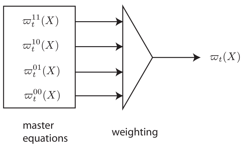
Figure 6: The expectation $\varpi_{t}(X)=\langle X(t)\rangle$ of the system operator $X(t)=j_{t}(X)$ when the system and field are initialized in the state $|\eta\rangle\langle\eta|\otimes\rho_{\mathrm{field}}$ may be calculated by weighting the solutions $\varpi_{t}^{jk}(X)$ from the single photon master equations (19).

III.7.2 The Stochastic Master Equation

Turning now to the problem of determining the filter, we again make use of the cascade extended system from Section III.4. Now we have

$$\varpi_{t}^{jk}(X)=\frac{\tilde{\varpi}_{t}(Q_{jk}\otimes X)}{w_{jk}(t)},$$ (50)

and so if we define the matrix

$$R(t)=\sum_{jk}\frac{\gamma_{jk}}{w_{jk}(t)}Q_{jk},$$ (51)

where $w_{jk}(t)$ and $Q_{jk}$ are as defined in Section III.4, we have (using (50), (48) and (27))

$$\varpi_{t}(X)=\tilde{\varpi}_{t}(R(t)\otimes X).$$ (52)

Note that the definition (27) of $\tilde{\varpi}_{t}(R(t)\otimes X)$ involves the ancilla system initialized in the excited state $|e\rangle=|\uparrow\rangle$.

The conditional expectation

$$\pi_{t}(X)=\mathbb{E}_{\eta\rho_{\mathrm{field}}}[X(t)\,|\,Y(s),0\leq s\leq t]$$ (53)

corresponding to the field in the state $\rho_{\mathrm{field}}$ is related to the conditional expectation $\tilde{\pi}_{t}(A\otimes X)$ for the extended system (see (34)) by the Bayes relation

$$\pi_{t}(X)=\frac{\tilde{\pi}_{t}(R(t)\otimes X)}{\tilde{\pi}_{t}(R(t)\otimes I)}.$$ (54)

Division by the denominator in (54) is needed to ensure the normalization $\pi_{t}(I)=1$. To prove (54), we need to show that $\tilde{\pi}_{t}(R(t)\otimes X)=\tilde{\pi}_{t}(R(t)\otimes I)\pi_{t}(X)$, or equivalently

$$\mathbb{E}_{\uparrow\eta 0}[\tilde{\pi}_{t}(R(t)\otimes X)c_{g}(t)]=\mathbb{E}_{\uparrow\eta 0}[\tilde{\pi}_{t}(R(t)\otimes I)\pi_{t}(X)c_{g}(t)]$$

for all choice of characteristic functions $c_{g}\left(t\right)$. However, $\mathbb{E}_{\uparrow\eta 0}[\tilde{\pi}_{t}(R(t)\otimes X)c_{g}(t)]$ equals $\mathbb{E}_{\uparrow\eta 0}[\tilde{U}^{{\dagger}}(t)(R(t)\otimes X\otimes I)\tilde{U}(t)c_{g}(t)]$, but by the extended system representation this is just $\mathbb{E}_{\eta\rho_{\mathrm{field}}}[X(t)c_{g}(t)]$ which in turn equals $\mathbb{E}_{\eta\rho_{f}}[\pi_{t}(X)c_{g}(t)]\equiv\mathbb{E}_{\uparrow\eta 0}[\tilde{U}^{{\dagger}}(t)(R(t)\otimes I)\tilde{U}(t)\pi_{t}(X)c_{g}(t)]$ which establishes the Bayes relation (54).

Since

$$\tilde{\pi}_{t}(R(t)\otimes X)=\sum_{jk}\gamma_{jk}\pi^{jk}_{t}(X),$$ (55)

where $\pi^{jk}_{t}(X)$ is defined by (36), the desired conditional expectation may be expressed as

$$\pi_{t}(X)=\frac{\sum_{j,k}\gamma_{jk}\pi^{jk}_{t}(X)}{\sum_{j,k}\gamma_{jk}\pi^{jk}_{t}(I)}.$$ (56)

Again, there is no differential equation for $\pi_{t}(X)$; instead it is computed from a normalized weighted sum, (56), and the filtering equations (37), Figure 7. The corresponding conditional density operator is given by

$$\rho(t)=\frac{\sum_{jk}\gamma_{kj}\rho^{jk}(t)}{\sum_{jk}\gamma_{kj}\mathrm{tr}\left\{\rho^{jk}(t)\right\}},$$ (57)

where the conditional quantities $\rho^{jk}(t)$ may be computed from the single photon filtering equations (44).

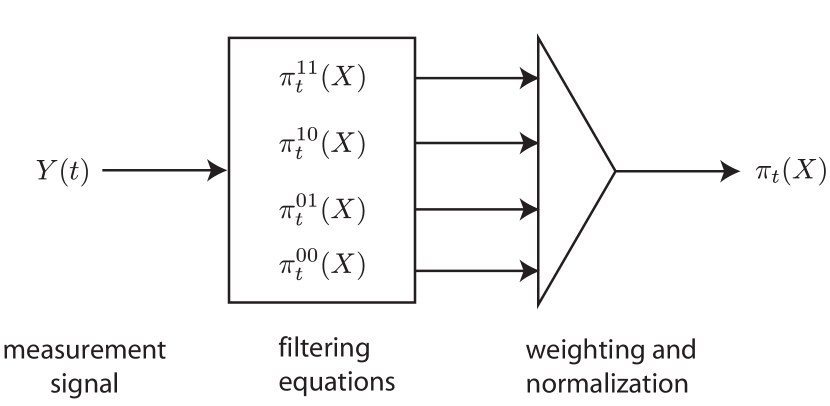
Figure 7: Relationship between the measured signal and the filtered estimate. The differential equations (37) must be integrated to compute $\pi_{t}^{jk}(X)$. Then depending on the state of the input field, the probe, these estimates must be weighted by the appropriate coefficients and normalized as specified in (56) to produce the desired conditional expectation $\pi_{t}(X)$.

These expressions allow filtering on any combination of a single photon and a vacuum state. One notable case it that of simple combination of one photon and vacuum ($\rho_{\mathrm{probe}}=p\left|{1}\right\rangle\!\left\langle{1}\right|+(1-p)\left|{0}\right\rangle\!\left\langle{0}\right|$) which is an experimentally accurate model for the output of the SPDC process LvoAicBen01 .

III.8 Illustrative Example of Single Photon Master and Filtering Equations

Here apply the filtering method derived above to the problem of exciting a two level atom, in free space, with a continuous mode single photon. This problem has received much attention recently StoAlbLeu07 ; WanSheSca10 ; StoAlbLeu10 ; RepSheFan10 . Until now it has only been possible to calculate ensemble averaged quantities. Here we show the individual trajectories associated with a particular experimental run.

This problem can be parametrized in our model as follows. We take the coupling operator to be $L=\sqrt{\kappa}\sigma_{-}$, the internal dynamics of the atom are specified by the Hamiltonian $H=0$ and there is no scattering i.e. $S=I$. Here $\kappa>0$ is the coupling rate (often referred to as the measurement strength) and is chosen to be $\kappa=1$. The atom is take to be in the ground state initially $\left|{g}\right\rangle\!\left\langle{g}\right|$, then a single photon in the wavepacket $\xi(t)$ interacts with the atom. We take the wavepacket to be a Gaussian parametrized as

$$\xi_{\rm gau}(t)=\left(\frac{\Omega^{2}}{2\pi}\right)^{1/4}\!\exp{\left[-\frac{\Omega^{2}}{4}(t-t_{c})^{2}\right]},$$ (58)

where $t_{c}$ specifies the peak arrival time and $\Omega$ is the frequency bandwidth of the pluse.

Now we wish to calculate the excited state population of the two level atom as a function of time. Other studies have only been able to calculate the master equation evolution of the atomic state StoAlbLeu07 ; WanSheSca10 ; StoAlbLeu10 ; RepSheFan10 . In our formalism this corresponds to propagating the master equations and taking the expectation

$$\mathbb{P}_{e}(t) ={\rm Tr}\left[{{\varrho^{11}(t)\left|{e}\right\rangle\!\left\langle{e}\right|}}\right],$$ (59)

where $\varrho^{11}(t)$ is the solution to Eq. (22). In Fig. 8 Eq. (59) is plotted, the dotted line (red), as a function of time for a two level atom interacting with a gaussian pulse. We choose $\Omega=1.46\kappa$ which is known to be optimal for excitation via a single photon in a Gaussian pulse StoAlbLeu07 ; WanSheSca10 ; StoAlbLeu10 . Our numerics agree with the prior results that $\max_{t}\mathbb{P}_{e}(t)\approx 0.8$ StoAlbLeu07 ; WanSheSca10 ; StoAlbLeu10 .

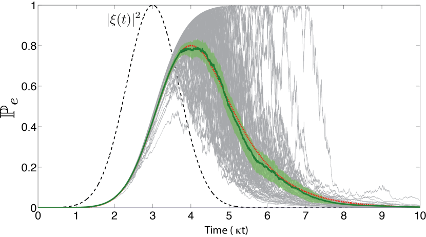
Figure 8: The excited state population, $\mathbb{P}_{e}$, of a two-level atom interacting with one photon in a Gaussian wavepacket. The dashed line is the Gaussian wavepacket $|\xi(t)|^{2}$ with bandwidth $\Omega=1.46\kappa$. The dotted (red) line is $\mathbb{P}_{e}$ as calculated by the master equation. The grey lines are the individual trajectories $\mathbb{P}_{e}^{c}$. The solid line is the ensemble average of sixty four trajectories plotted with error bars (the shaded light green region).

However, in our formalism we can also calculate the conditional state of the system using the quantum filtering equations derived above. The conditional excited state population is denoted by

$$\mathbb{P}_{e}^{c}(t) ={\rm Tr}\left[{{\rho^{11}(t)\left|{e}\right\rangle\!\left\langle{e}\right|}}\right],$$ (60)

where $\rho^{11}(t)$ is the solution to the filtering equations Eq. (44) or Eq. (45) for homodyne or photon counting measurements respectively. In what follows we will focus on the homodyne measurement filtering equations i.e. Eq. (44).

In Fig. 8, 64 different trajectories given by Eq. (60) are plotted as grey lines. For this particular bandwidth there is very little spread in the trajectories for $t<3$. After the bulk of the wavepacket has passed, at $t=4$, many of the trajectories start to decay, as evidenced by the many grey lines below $\mathbb{P}_{e}^{c}=0.5$ for $t>4$. Nevertheless there are a number of trajectories which continue to rise towards $\mathbb{P}_{e}^{c}=1$ for $t>4$. This means in a particular run of an experiment the atom may become fully excited. Such behavior can not be seen through the master equation approach of Refs. StoAlbLeu07 ; WanSheSca10 ; StoAlbLeu10 ; RepSheFan10 .

It is possible to confirm the consistency of the trajectories with the master equation solution by calculating a numerical average of the trajectories. We plot the ensemble average of the trajectories as the solid line in Fig. 8 with error bars smeared around this line. The numerically calculated ensemble average agrees with the master equation behavior given that a small ensemble was used to calculate this mean value.

IV Superposition of Coherent Field States

In this section we turn to the problem of determining the master equation and the quantum filter for systems drive by a boson field whose state is a superposition of continuous-mode coherent states. In section IV.1 we describe continuous-mode coherent states and superpositions of them, as well as the action of the quantum noises on such states. Section IV.2 is devoted to the derivation of the master equation for superpositions of coherent states. In section IV.3 we develop a cascaded system signal model. This model allows us to use the methodology from Section III, with appropriate changes due to the nature of the superposition of coherent states, to derive the filtering equations in section IV.4. Then we give the filter for the case of photon counting in section IV.5 and generalize to mixed input states.

IV.1 Superpositions and Combinations of Coherent States

Typically single mode coherent states of a field are denoted by $\left|{\alpha}\right\rangle$. In this paper we shall often refer to a superposition of continuous-mode coherent states as a (continuous-mode) cat-state Lou_book00 ; GarChi_book08 . Formally, the superpositions of continuous-mode coherent states is given by

$$|\psi\rangle=\sum_{j=1}^{n}s_{j}|\alpha_{j}\rangle,$$ (61)

where $|\alpha_{j}\rangle$ are coherent states, determined by functions $\alpha_{j}(t)$ with $\alpha_{j}\neq\alpha_{k}$ if $j\neq k$. The superposition weights $s_{j}$ are complex numbers such that $\langle\psi|\psi\rangle=\sum_{j,k}s_{j}^{\ast}s_{k}\langle\alpha_{j}|\alpha_{k}\rangle=1$ (i.e., $\psi$ is normalized and is a pure state vector of the field). Given a function $\alpha$, the coherent state $|\alpha\rangle$ of a continuous-mode field is given by the displacement or Weyl operator $D(\alpha)$ applied to the vacuum state of the continuous-mode field:

$$|\alpha\rangle=D(\alpha)|0\rangle.$$ (62)

The inner product of two coherent states $|\alpha\rangle$, $|\beta\rangle$ in the Fock space is given by

$$\langle\alpha|\beta\rangle=\exp\Big{(}-\frac{1}{2}\parallel\alpha\parallel^{2}-\frac{1}{2}\parallel\beta\parallel^{2}+\langle\alpha,\beta\rangle\Big{)},$$ (63)

where $\langle g,f\rangle=\int_{-\infty}^{\infty}g(s)^{*}f(s)ds$ and $\parallel\!\cdot\!\parallel=\langle\cdot,\cdot\rangle$ are the $L^{2}$ inner product and norm, respectively. The normalization condition for the superposition state (61) means that the coefficients must satisfy $\sum_{j,k}s_{j}^{\ast}s_{k}g_{jk}=1$, where $g_{jk}=\langle\alpha_{j}|\alpha_{k}\rangle$.

More generally, we may consider a field density operator

$$\rho_{\mathrm{field}}=\sum_{jk}\gamma_{kj}|\alpha_{j}\rangle\langle\alpha_{k}|,$$ (64)

that generalizes the superposition state $|\psi\rangle$ to allow for statistical combinations of coherent states. The normalization for the state $\rho_{\mathrm{field}}$ is $\sum_{j,k}\gamma_{jk}g_{jk}=1$.

In what follows the action of the quantum noises $dB$ and $d\Lambda$ on coherent states will be important:

$$dB(t)|\alpha\rangle = \alpha(t)|\alpha\rangle dt,$$

$$d\Lambda(t)|\alpha(t)\rangle = dB^{\ast}(t)\alpha(t)|\alpha\rangle.$$ (65)

IV.2 Master Equation for Systems Driven by a Field in a Combination or Superposition of Coherent States

Again, before we derive the master equation we introduce some notation that helps to formulate the master equation. Recall that we defined the asymmetric expectation $\mathbb{E}_{jk}\left[{X\otimes F}\right]\equiv\langle\eta|X|\eta\rangle\langle\phi_{j}|F|\phi_{k}\rangle$. In section III we took the field states $|\phi_{j}\rangle,|\phi_{k}\rangle$ to be either vacuum or one photon. In this section we use this same notation but the field states are understood to be continuous-mode coherent states i.e. $|\alpha_{j}\rangle,|\alpha_{k}\rangle$. The indices $j,k$ now take the values $1,\ldots,n$.

The expectation of an arbitrary system observable, with respect to the state $|\eta\rangle\langle\eta|\otimes\rho_{\mathrm{field}}$, at time $t$ is

$$\varpi_{t}(X)=\mathbb{E}_{\eta\rho_{\mathrm{field}}}[X(t)].$$ (66)

Using the notation (similar to the single photon case)

$$\varpi_{t}^{jk}(X)=\mathbb{E}_{jk}\left[{X(t)}\right]=\langle\eta\alpha_{j}|X(t)|\eta\alpha_{k}\rangle,$$ (67)

with $\rho_{\mathrm{field}}$ as given in 64, we may write  (66) as

$$\varpi_{t}(X)=\sum_{jk}\gamma_{jk}\varpi_{t}^{jk}(X).$$ (68)

As in section III.2, we can derive the Heisenberg master equation by taking the expectation of the equation of motion for an arbitrary system operator $dX(t)$, i.e.  (4). Doing so yields the equations

$$\dot{\varpi}_{t}^{jk}(X)=\varpi_{t}^{jk}(\mathcal{G}_{t}^{jk}X),$$ (69)

where we define a new superoperator

$$\mathcal{G}_{t}^{jk}X \equiv \mathcal{L}X+S^{{\dagger}}[X,L]\alpha_{j}^{\ast}(t)+[L^{{\dagger}},X]S\alpha_{k}(t)$$ (70)

$$+(S^{{\dagger}}XS-X)\alpha_{j}^{\ast}(t)\alpha_{k}(t),$$

with initial conditions $\varpi_{0}^{jk}(X)=\langle\eta|X|\eta\rangle g_{jk}$. Note that equations (69) are uncoupled.

The corresponding density operator is

$$\varrho(t)=\sum_{jk}\gamma_{jk}\varrho^{jk}(t)$$ (71)

where

$$\dot{\varrho}^{jk}=\mathcal{G}_{t}^{jk\star}[\varrho^{jk}] \equiv \mathcal{L}^{\star}\varrho+[S\varrho^{jk},L^{{\dagger}}]\alpha_{j}(t)+[L,\varrho S^{{\dagger}}]\alpha_{k}^{\ast}(t)$$ (72)

$$+(S\varrho^{jk}S^{{\dagger}}-\varrho^{jk})\alpha_{j}(t)\alpha_{k}^{\ast}(t),$$

and $\varrho^{jk}(0)=\left|{\eta}\right\rangle\!\left\langle{\eta}\right|{g_{jk}}$.

The master equations (69) and (72) consist of a weighted sum of cross-expectations. Clearly these equations reduce to the vacuum master equation if the only term in the superposition or combination is the vacuum.

IV.3 Extended System

In this section we describe a cascade extended system $G_{T}=G\triangleleft M$ that will be used in section IV.4 to determine the quantum filtering equations for the mixed or superposition of coherent state field. The ancilla system $M$ will be an $n$-level system, with orthonormal basis $|j\rangle$, $j=1,\ldots,n$. The parameters for this system are

$$M=(I,L_{M},0),$$

where

$$L_{M}=\sum_{j}\alpha_{j}(t)|j\rangle\langle j|,$$ (73)

and we take the initial state of the ancilla to be the density matrix

$$\rho_{a}=\frac{1}{N_{a}}\sum_{jk}\gamma_{kj}|j\rangle\langle k|,$$ (74)

where $N_{a}=\sum_{l}\gamma_{ll}$ is a normalization factor. The extended system is

$$G_{T}=G\triangleleft M=(S,L+SL_{M},H+\mathrm{Im}\left\{L^{{\dagger}}SL_{M}\right\}).$$

Define $Q_{jk}=|j\rangle\langle k|$. Then a straightforward calculation shows that

$$\mathcal{L}_{L_{M}}(Q_{jk})=m_{jk}(t)Q_{jk},$$ (75)

where

$$m_{jk}(t)=\alpha_{j}^{\ast}(t)\alpha_{k}(t)-\frac{1}{2}|\alpha_{j}(t)|^{2}-\frac{1}{2}|\alpha_{k}(t)|^{2}.$$ (76)

Now consider the extended system $G_{T}$ initialized in the state $\rho_{a}\otimes|\eta\rangle\langle\eta|\otimes|0\rangle\langle 0|$ (driven by vacuum $|0\rangle$). Then the methods used in Sections III.4 and III.7 may be adapted to the present case to show that

$$\varpi_{t}^{jk}(X)=\frac{\tilde{\varpi}_{t}(Q_{jk}\otimes X)}{w_{jk}(t)},$$ (77)

where $w_{jk}(t)$ is defined to be the solution of

$$\dot{w}_{jk}(t)=m_{jk}(t)w_{jk}(t),\ \ w_{jk}(0)=\frac{1}{N_{a}g_{jk}},$$ (78)

and

$$\mathbb{E}_{\eta\rho_{\mathrm{field}}}[X(t)]=\mathbb{E}_{\rho_{a}\eta 0}[\tilde{U}^{{\dagger}}(t)(R(t)\otimes X)\tilde{U}(t)],$$ (79)

where

$$R(t)=\sum_{j,k}\frac{\gamma_{jk}}{w_{jk}(t)}Q_{jk},$$ (80)

These expressions are very similar to the photon case, but with some important differences. For instance, the ancilla was initialized in the excited state for the photon case, while here for the mixed coherent case the initial ancilla state is the density $\rho_{a}$.

IV.4 The Stochastic Master Equation (Filter) for Amplitude Quadrature Measurements

The quantum filter for the general combination of coherent state case may now be derived in exactly the same way as was done for the combination of single photon and vacuum in Section III.7. The conditional expectation we are interested in is

$$\pi_{t}(X)=\mathbb{E}_{\eta\rho_{\mathrm{field}}}[X(t)\,|\,Y(s),0\leq s\leq t],$$ (81)

where now $\rho_{\mathrm{field}}$ is given by (64). Equations (54), (56), and (57) again hold, but with modifications to the terms as described above. The filtering equations are as follows.

The conditional quantities $\pi_{t}^{jk}(X)$ satisfy the coupled system of equations

$$d\pi_{t}^{jk}(X)=\pi_{t}^{jk}(\mathcal{G}^{jk}X)dt+\mathcal{H}_{t}^{jk}\left(X\right)dW(t)$$

where the innovations process $W(t)$ is a Wiener process and is given by

$$dW(t)= dY(t)$$

$$-\sum_{l}\frac{\gamma_{ll}}{N_{a}}\pi_{t}^{ll}(L+S\alpha_{l}(t)+L^{{\dagger}}+S^{{\dagger}}\alpha_{l}^{\ast}(t))dt.$$

and the new superoperator $\mathcal{H}_{l}^{jk}\left(\cdot\right)$ is defined by

$$\mathcal{H}_{l}^{jk}\left(X\right)$$

$$\!\equiv\pi_{t}^{jk}\big{(}X(L+S\alpha_{k}(t))+(L^{{\dagger}}+S^{{\dagger}}\alpha_{j}^{\ast}(t))X\big{)}$$

$$\quad\!-\pi_{t}^{jk}(X)\sum_{l}\frac{\gamma_{ll}}{N_{a}}\pi^{ll}({L+L^{{\dagger}}+S\alpha_{l}(t)+S^{{\dagger}}\alpha_{l}^{\ast}(t))}.$$

As before, we may write $\pi_{t}^{jk}(X)=\mathrm{tr}\left\{{\varrho}^{jk}(t)^{{\dagger}}X\right\}$, where $\varrho^{jk}(t)$ satisfies the coupled differential equations (for $j,k=1,2,\ldots,n$):

$$d\rho^{jk}(t)=\mathcal{G}_{t}^{jk\star}[\rho^{jk}(t)]dt+\mathcal{H}_{t}^{jk\star}\left[{\rho^{jk}(t)}\right]dW(t)$$ (82)

where

$$\mathcal{H}_{t}^{jk\star}\left[{\rho^{jk}}\right]\equiv (L+S\alpha_{k}(t))\rho^{jk}+\rho^{jk}(L^{{\dagger}}+S^{{\dagger}}\alpha_{j}^{\ast}(t))$$

$$-\rho^{jk}\sum_{l} \frac{\gamma_{ll}}{N_{a}}\mathrm{tr}\left[{{(L+L^{{\dagger}}+S\alpha_{l}(t)+S^{{\dagger}}\alpha_{l}^{\ast}(t))\rho^{ll}}}\right],$$

with initial conditions $\rho_{0}^{jk}(t)=|\eta\rangle\langle\eta|g_{jk}$ (recall that $g_{jk}=\langle\alpha_{j}|\alpha_{k}\rangle$). The conditional density operator is given by (57), with the $\rho^{jk}(t)$ given instead by (82).

We remark that the innovations for the cat case now depends on the weights, in contrast to the mixed photon/vacuum case.

IV.5 The Stochastic Master Equation (Filter) for Photon Counting Measurements

Analogously, we may also compute the quantum filtering equations for a system driven by a coherent superposition in the case where the measurement performed on the output field, $Y(t)$, is photon counting. The filtering equations in the Heisenberg form are given by (for $j,k=1,2,\ldots,n$):

$$d\pi^{jk}_{t}(X) = \pi^{jk}_{t}(\mathcal{G}^{jk}(X))dt+\biggl{(}\frac{\pi_{t}^{jk}(L^{\dagger}XL+\alpha_{k}(t)L^{\dagger}XS+\alpha_{j}^{*}(t)S^{\dagger}XL+\alpha_{j}^{*}(t)\alpha_{k}(t)S^{\dagger}XS)}{\sum_{j=1}^{n}\frac{\gamma_{jj}}{N_{a}}\pi_{t}^{jj}(L^{\dagger}L+\alpha_{j}(t)L^{\dagger}S+\alpha_{j}^{*}(t)S^{\dagger}L+|\alpha_{j}|^{2}I)}-\pi_{t}^{jk}(X)\biggr{)}dN(t),$$

where

$$dN(t) = dY(t)-\sum_{j=1}^{n}\frac{\gamma_{jj}}{N_{a}}\pi_{t}^{jj}(L^{\dagger}L+\alpha_{j}(t)L^{\dagger}S+\alpha_{j}^{*}(t)S^{\dagger}L+|\alpha_{j}(t)|^{2}I)dt,$$ (83)

and with initial conditions $\pi_{0}^{jk}(X)=\langle\eta|X|\eta\rangle g_{jk}$. The corresponding Schrödinger-picture filter is

$$d\rho^{jk}(t) = \mathcal{G}_{t}^{jk\star}[\rho^{jk}]dt+\biggl{(}\mathcal{N}^{-1}[L\rho^{jk}L^{\dagger}+\alpha_{k}(t)S\rho^{jk}L^{\dagger}+\alpha_{j}^{*}(t)L\rho^{jk}S^{\dagger}+\alpha_{j}^{*}(t)\alpha_{k}(t)S\rho^{jk}S^{\dagger})]-\rho^{jk}\biggr{)}dN(t),$$

where

$$\mathcal{N}=\sum_{j=1}^{n}\frac{\gamma_{jj}}{N_{a}}{\rm Tr}\left[{{\rho^{jj}(L^{\dagger}L+\alpha_{j}(t)L^{\dagger}S+\alpha_{j}^{*}(t)S^{\dagger}L+|\alpha_{j}|^{2}I)}}\right]$$ (84)

and $dN(t)=dY(t)-\mathcal{N}dt$, with initial conditions $\rho^{jk}(0)=\left|{\eta}\right\rangle\!\left\langle{\eta}\right|g_{jk}$.

V Conclusion

We have shown that quantum filtering may be extended beyond the Gaussian input situation to consider a range of non-classical states that are of current interest. Photon wave packet shaping is already being applied experimentally and our filtering equations for the single photon input completes the problem addressed by Gheri et al. in GheEllPelZol99 by giving the quantum trajectories associated to the master equation they derive. We extend this general combinations of the vacuum an a one photon state through a straightforward weighting procedure. The filter equations themselves have potential applications to areas such as shaping wave packet for maximal / minimal absorption by, for instance, a two level atom, or to controlling the system so as to shape the outgoing field.

We have also derived the quantum filter for cat states. While the concept of an environment being in a superposition of states may seem unphysical from the perspective of macroscopic superselection rules, as we have seen this may effectively be what happens internally once a standard input is first fed through an appropriate filter system $M$. This leads naturally to questions of decoherence Kupsch97 , and whether preparing input in a cat state is advantageous in preventing decoherence of cat states for a given system. It is now experimentally possible to isolate quantum systems sufficiently well to create cat states in a laboratory NeeNieHet06 ; OurTuaLau06 ; OurHyuTua07 . The cat-state filtering equation will be of importance for investigating questions as to whether such superpositions may protected via appropriate environment engineering.

Acknowledgements. The authors wish to thank J. Hope for helpful discussions and for pointing out reference single-photon-production to us. We also wish to thank A. Doherty, H. Wiseman, E. Huntington and an anonymous referee (of an earlier version of this manuscript) for helpful discussions and suggestions; G. Zhang for carefully reading and earlier version of this manuscript; and B. Baragiola for discussions about sec. III H. MJ and HIN gratefully acknowledge the support of the Australian Research Council. JC acknowledges support from National Science Foundation Grant No. PHY-0903953 and Office of Naval Research Grant No. N00014-11-1-008. JG gratefully acknowledges the support of the UK Engineering and Physical Sciences Research Council through Research Project EP/H016708/1

References

- (1) A. I. Lvovsky, H. Hansen, T. Aichele, O. Benson, J. Mlynek, and S. Schiller, Phys. Rev. Lett. 87, 050402 (2001).
- (2) J. S. Neergaard-Nielsen, B. Melholt Nielsen, C. Hettich, K. Mølmer, and E. S. Polzik, Phys. Rev. Lett. 97, 083604 (2006).
- (3) A. Ourjoumtsev, R. Tualle-Brouri, J. Laurat, and P. Grangier, Philippe, Science 312, 83 (2006).
- (4) A. Ourjoumtsev, H. Jeong, R. Tualle-Brouri, and P. Grangier, Philippe, Nature 448, 784 (2007).
- (5) A. Kuhn, M. Hennrich, and G. Rempe, Phys. Rev. Lett. 87, 067901 (2002).
- (6) J. McKeever, A. Boca, A. D. Boozer, R. Miller, J. R. Buck, A. Kuzmich, and H. J. Kimble, Science 303 1992 (2004).
- (7) Z. Yuan, B. E. Kardynal, R. M. Stevenson, A. J. Shields, C. J. Lobo, K. Cooper, N. S. Beattie, D. A. Ritchie, and M. Pepper, Science 295, 102 (2002).
- (8) C. Eichler, D. Bozyigit, C. Lang, L. Steffen, J. Fink, and A. Wallraff, Phys. Rev. Lett. 106, 220503 (2011).
- (9) E. Knill, R. LaFlamme, and G. J. Milburn, Nature (London) 409, 46 (2001).
- (10) T. C. Ralph, A. Gilchrist, and G. J. Milburn, Phys. Rev. A 68, 042319 (2003).
- (11) N. Gisin, G. Ribordy, W. Tittel, and H. Zbinden, Reviews of modern physics, 74, 145 (2002).
- (12) J. I. Cirac, P. Zoller, H. J. Kimble, and H. Mabuchi, Phys. Rev. Lett. 78, 3221 (1997).
- (13) V. P. Belavkin, In Lecture notes in Control and Inform Sciences 121, 245–265, Springer–Verlag, Berlin 1989.
- (14) V. P. Belavkin, In Stochastic Methods in Mathematics and Physics 310–324, World Scientific, Singapore 1989.
- (15) P. Staszewski and G. Staszewska, Open Systems & Information Dynamics, 3, 275 (1995).
- (16) A. Barchielli and V. P. Belavkin, Phys. A Math. Gen. 24, 1495 (1991).
- (17) J.E. Gough, A. Sobolev, Open Sys. & Inf. Dynamics, 11, 1-21, (2004)
- (18) L. Bouten, M. Guta, and H. Maassen, J. Phys. A: Math. and Gen. 37, 3189 (2004).
- (19) L. Bouten, R. van Handel and M. R. James, SIAM Journal on Control and Optimization 46, 2199 (2007).
- (20) J. Gough, C. Köstler, Commun. Stoch. Anal., 4, No. 4, 505-521 (2010)
- (21) R.L Stratonovich, Radio Engineering and Electronic Physics, 5:11, pp.1-19, (1960).
- (22) H. J. Carmichael. An open systems approach to quantum optics (Springer: lecture notes in physics vol. 18, 1993).
- (23) J. Dalibard, Y. Castin, and K. Mølmer, Phys. Rev. Lett. 68, 580 (1992).
- (24) N. Gisin and I. C. Percival, J. Phys. A: Math. Gen. 25, 567 (1992).
- (25) R. Drum, A. S. Parkins, P. Zoller, and C. W. Gardiner, Phys. Rev. A 46, 4382 (1992).
- (26) C. W. Gardiner and P. Zoller. Quantum Noise (Springer Berlin, 2000).
- (27) C. W. Gardiner and M. J. Collett, Phys. Rev. A 31, 3761 (1985).
- (28) S. M. Tan, D. F. Walls, and M. J. Collett, Phys. Rev. Lett. 66, 252-255 (1991)
- (29) H. M. Wiseman and G. J. Milburn, Quantum Measurement and Control, (Cambridge Univ. Press, Cambridge, 2010)
- (30) G. J. Milburn W. J. Munro, K. Nemoto and S. L. Braunstein, Phys. Rev. A 66, 023819 (2002).
- (31) W. J. Munro, T. C. Ralph, S. Glancy, S. L. Braunstein, A. Gilchrist, K. Nemoto, and G. J. Milburn, Journal of Optics B: Quantum and Semiclassical Optics, 6, 828 (2004).
- (32) M. Yanagisawa and H. Kimura, IEEE Trans. Automat. Control 48, 2107 (2003), and M. Yanagisawa and H. Kimura, IEEE Trans. Automat. Control 48, 2121 (2003).
- (33) J. Gough, M. R. James, Commun. Math. Phys. 287, 1109 (2009).
- (34) J. Gough, M. R. James, IEEE Trans. on Automatic Control 54, 2530 (2009).
- (35) R. L. Hudson and K. R. Parthasarathy, Commun. Math. Phys. 93, 301 (1984).
- (36) K.R. Parthasarathy. An introduction to quantum stochastic calculus (Birkhauser, 1992).
- (37) V. Belavkin, Theory Probab. Appl. 38, 573 (1994)
- (38) B.D.O Anderson, J. Moore, Optimal Filtering, (Prentice-Hall, 1979)
- (39) C. W. Gardiner, Phys. Rev. Lett. 70, 2269 (1993).
- (40) H. J. Carmichael, Phys. Rev. Lett. 70, 2273 (1993).
- (41) K. M. Gheri, K. Ellinger, T. Pellizzari, and P. Zoller, Fortschr. Phys. 46, 401 (1998).
- (42) J. Gough, M. James, and H. Nurdin, Quantum master equation and filter for systems driven by fields in a single photon state, IEEE Conference on Decision and Control, (2011).
- (43) M. G. Raymer, J. Noh, K. Banaszek and I. A. Walmsley, Phys. Rev. A 72, 023825 (2005); A. M. BrańczykT. C. Ralph, W. Helwig and C. Silberhorn, New Journal of Physics 12, 063001 (2010).
- (44) R. Loudon, The Quantum Theory of Light, 3rd ed. (Oxford University Press, Oxford, 2000).
- (45) G. J. Milburn, in Springer Handbook of Lasers and Optics, edited by F. Träger (Springer, 2007) Chap. 14, pp. 1053 -1078.
- (46) G. J. Milburn, Eur. Phys. J. Special Topics 159, 113 (2008).
- (47) B. Lounis and M. Orrit, Rep. Prog. Phys. 68, 1129 (2005); S. Scheel, Journal of Modern Optics 56, 141 (2009).
- (48) J. Kupsch, J. Kupsch, in Decoherence and the Appearance of a Classical World in Quantum Theory, edited by D. Guilini et al. (Springer, Berlin, 1997).
- (49) J.C. Garrison, R.Y. Chiao, Quantum optics, (Oxford University Press, 2008).
- (50) M. Stobińska, G. Alber, and G. Leuchs, EPL 86, 14007 (2009).
- (51) Y. Wang, J. Minář, L. Sheridan, and V. Scarani, Phys. Rev. A 83, 063842 (2011).
- (52) M. Stobińska, G. Alber, and G. Leuchs, Chapter 8 - Quantum Electrodynamics of One-Photon Wave Packets Pages 457-483, in Unstable States in the Continuous Spectra, Part I: Analysis, Concepts, Methods, and Results, Edited by Cleanthes A. Nicolaides and Erkki Br ndas, Volume 60, Pages 1-549 (2010). Also available as arXiv:1002.3059v2.
- (53) E. Rephaeli, Jung-Tsung Shen, and S. Fan, Phys. Rev. A 82, 033804 (2010).