Numerical study of fluxon solutions of sine-Gordon equation under the influence of the boundary conditions

Abstract

The fluxon solutions of a boundary problem for the sine-Gordon equation (SGE) are investigated numerically in dependence on the boundary conditions. Interconnection between fluxon and constant solutions is analyzed. Numerical results are discussed in context of the long Josephson junction model.

1 Introduction

The sine-Gordon equation is a nonlinear hyperbolic partial differential equation involving the d’Alembert operator and the sine of the unknown function. The equation reads

$$u_{tt}-u_{xx}+\sin u=0\,,$$ (1)

where $u=u(x,t)$. It arises in differential geometry and various areas of physics, including applications in relativistic field theory, Josephson junctions (JJs) or mechanical transmission lines. The stack of coupled JJs describing by system of coupled sine-Gorgon equations is investigating very intensively today [1, 2, 3].

In the framework of the long JJs model, the dynamics of the magnetic flux in a JJ of length $2l$ is described by the perturbed sine-Gordon equation:

$$\varphi_{xx}-\varphi_{tt}-\alpha\varphi_{t}=\sin\varphi-\gamma\,,\quad t>0\,,\quad x\in(-l,l)$$ (2)

with boundary conditions

$$\varphi_{x}(\pm l,t)=h_{e}\,,$$ (3)

where $\varphi$ is the magnetic flux distribution, $h_{e}$ – the external magnetic field, $\gamma$ – the external current and $\alpha\geq 0$ – the dissipation coefficient.

The aim of this work is a numerical investigation of the properties of the static fluxon solutions of Eq.(2) under the influence of the external magnetic field parameter $h_{e}$ in (3). Such solutions satisfy the following boundary problem

$$-\varphi_{xx}+\sin\varphi-\gamma=0,\quad x\in(-l;l),\quad\varphi_{x}(\pm l)=h_{e}\,.$$ (4)

Here, we only consider the case of the JJ length $2l=10$ with zero external current $\gamma=0$.

2 Numerical approach

The static fluxon solutions of Eq.(2) are obtained numerically, by solving of the boundary problem (4). The stability analysis is based on numerical solution of the following Sturm-Liouville problem [4]

$$-\psi_{xx}+q(x)\psi=\lambda\psi,\quad\psi_{x}(\pm l)=0,\quad q(x)=\cos\varphi(x,p),\quad p=(l,h_{e},\gamma).$$ (5)

In this approach, the minimal eigenvalue of Eq.(5) $\lambda_{0}(p)>0$ corresponds to a stable solution. In case $\lambda_{0}(p)<0$ solution $\varphi(x,p)$ is unstable. The case $\lambda_{0}(p)=0$ indicates a bifurcation with respect to one of parameters $p=(l,h_{e},\gamma)$.

The numerical solving of Eq.(4) is based of the continuous analog of Newton’s method [5]. At each Newtonian iteration the corresponding linearized problem is solved, on a uniform grids with $1025$ number of nodes, using a three-point Numerov approximation of the fourth order accuracy [6].

For numerical solution of the Sturm-Liouville problem (5) we applied the standard three-point second order finite-difference formulae. First several eigenvalues of the resulting algebraic three-diagonal eigenvalue problem are obtained by means of the standard EISPACK code. Details of numerical scheme are described in [7, 8, 9] for the double sine-Gordon equation.

The known for $h_{e}=0$ solutions $M_{0}$ and $\Phi^{1}$ are numerically path-followed to non-zero positive $h_{e}$. At each $i$th step of the numerical continuation we analyze the stability of solution $\varphi(x,h_{e}^{(i)})$ and calculate the following physical characteristics:

• full magnetic flux of the distribution $\Delta\varphi^{(i)}\varphi=\varphi(l,h_{e}^{(i)})-\varphi(-l,h_{e}^{(i)})$;

• quantity $N$ denoted “number of fluxons” in [7] and determined as follows

  $$N[\varphi(x,h_{e}^{(i)})]=\frac{1}{2l\pi}\int\limits_{-l}^{l}\varphi(x,h_{e}^{(i)})\,dx.$$ (6)

Note, since each solution $\varphi$ of Eq.(4) is defined with an accuracy $2k\pi$ ($k\in\mathbf{Z}$) then the value $N[\varphi]$ is also defined with accuracy $2k$. The arbitrariness at the choice of integer number $k$ can be used for the “concordance” of the value $N$ with the value of the full magnetic flux $\Delta\varphi$ according to the condition

$$\left|N[\varphi]-\Delta\varphi/2\pi\right|\rightarrow\min.$$ (7)

Below, as in [7, 8, 9, 11], solutions $\varphi$ with $n=N$ where N satisfies Eq.(7) are denoted $\varphi^{n}$.

The crossing through the turning points in the numerical continuation (where the direction of the moving along the curve $\Delta\varphi(h_{e})$ changes as we follow on the new branch) was organized as in [10]. The turning points are identified with help of the relation that is tested at each $i$th step of numerical continuation:

$$\left|\frac{{h_{e}}^{(i)}-{h_{e}}^{({i-1})}}{\Delta\varphi^{(i)}-\Delta\varphi^{(i-1)}}\right|<\varepsilon.$$ (8)

where $\varepsilon>0$ is small known quantity. Note that (8) is a simple approximation of equality $dh_{e}/d\Delta\varphi=0$ that is valid at the turning points of the curve $\Delta\varphi(h_{e})$. In case we run into a turning point the sign of $h_{e}$-increment should be changed. At each step of the numerical continuation, the initial guess for Newtonian process was chosen in the form

$$\varphi(h_{e}^{(i+1)})=\varphi(h_{e}^{(i)})+(h_{e}^{(i+1)}-h_{e}^{(i)})\cdot\frac{\varphi(h_{e}^{(i)})-\varphi(h_{e}^{(i-1)})}{h_{e}^{(i)}-h_{e}^{(i-1)}}$$ (9)

that prevents the continuation from reversing to the previous branch of $\Delta\varphi(h_{e})$.

3 Numerical results

Figure 1: Internal magnetic field distribution $\varphi_{x}(x)$ associated with the state $M_{0}$ for several values of the magnetic field $h_{e}$.

Figure 2: Internal magnetic field distribution $\varphi_{x}(x)$ associated with the state $\Phi^{1}$ for several values of magnetic field $h_{e}$.

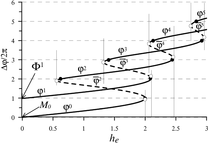
Figure 3: Dependence of the full magnetic flux $\Delta\varphi$ on the magnetic field $h_{e}$ for fluxon distributions associated with $M_{0}$ and $\Phi^{1}$. Solid and dashed lines correspond, respectively, stable and unstable states. Light circles indicate the turning points, dark circles indicate the points where solution changes its stability.

Figure 4: Dependence of the minimal eigenvalue $\lambda_{0}$ on the magnetic field $h_{e}$ for the branch associated with $\Phi^{1}$. Light circles indicate the turning points, dark circles indicate the points of stability change.

Figure 5: Dependence of the minimal eigenvalue $\lambda_{0}$ on the magnetic field $h_{e}$ for the branch associated with $M_{0}$. Light circles indicate the turning points, dark circles indicate the points of stability change.

Figure 6: Coexisting stable internal magnetic field distributions $\varphi_{x}$ at magnetic field $h_{e}=1$.

Figure 7: Coexisting stable internal magnetic field distributions $\varphi_{x}$ at magnetic field $h_{e}=2$.

Two basic distributions are known at $h_{e}=0$: the uniform Meissner solution $M_{0}$ with $N[M_{0}]=0$ and the fluxon solution $\Phi^{1}$ with $N[\Phi^{1}]=1$ ([7]). Minimal eigenvalue $\lambda_{0}$ of Eq.(5) is negative for $\Phi^{1}$ and positive for $M_{0}$. As we continue basic state $M_{0}$ to $h_{e}>0$ $\lambda_{0}$ stays positive, i.e. the branch is stable until $h_{e}=2$. In the $\Phi^{1}$ case, the minimal eigenvalue $\lambda_{0}$ crosses zero at the point $h_{e}=h_{1}=0.054$, i.e. the branch is unstable for $0\leq h_{e}\leq h_{1}$ and stable for $h_{1}<h_{e}<2.098$. Transformation of the internal magnetic field shape of basic solutions in dependence on $h_{e}$ is shown on Figs.2, 2.

The $\Delta\varphi(h_{e})$ branches associated with the basic solutions $M_{0}$ and $\Phi^{1}$ are presented on Fig.3. It is seen, at some points (light circles in Fig.3) the curves $\Delta\varphi(h_{e})$ turn back to another, upper, branches. When the $\Delta\varphi(h_{e})$ curve turns to the left (“$\supset$”-point) the quantity $N$ is increased to $N+2$. So, the branch started from the basic $M_{0}$ solution at $h_{e}=0$, joins the fluxons (stable and unstable) with the even $N$ while the another branch (associated with the $\Phi^{1}$ basic fluxon) connects fluxons (stable and unstable) with the odd $N$.

The change of stability occurs at the points (marked by dark circles in Fig.3) where the $\lambda_{0}(h_{e})$ curve crosses zero, see Figs.5,5. The “${\supset}$”- and “$\subset$”-turning points are indicated by the light circles. The “$\subset$”-turning points connect a pair of unstable solutions with the same number $N$: $\varphi^{n}$ and $\bar{\varphi}^{n}$. An increasing $N$ to $N+2$ is observed at the “${\supset}$”-turning points (light circles).

Thus, for $0<h_{e}<h_{1}$ we have a single stable static distribution (associated with the basic solution $M_{0}$). For $h_{1}<h_{e}<h_{cr}$, $h_{cr}=0.561$ this distribution coexist with another one associated with the basic solution $\Phi^{1}$. An increasing of magnetic field $h_{e}$ leads appearing, at $h_{cr}$, (most left light circle in Fig.3) a pair of (unstable) states ($\varphi^{2}$, $\bar{\varphi}^{2}$). As $h_{e}$ is growing next, the stabilization of $\bar{\varphi}^{2}$ occurs (most left dark circle in Fig.3), i.e. for $h_{e}=1$ we have three stable distributions to be coexisting with unstable state $\varphi^{2}$, see Fig.7. Further increasing $h_{e}$ induces a creation, at each “$\subset$”-point, of additional pair ($\varphi^{n}$, $\bar{\varphi}^{n}$) with growing $n$, see Fig.7. At the same time, the pairs $(\varphi^{n},\bar{\varphi}^{n+2})$ with previous values $n$ are sequentially disappearing at the “$\supset$”-points.

4 Conclusions

The detailed information on the variation of fluxon structure with external magnetic field in long Josephson junction is very important for correct interpretation of the experimental results. In this paper we investigated stationary fluxon solutions of Eq.(2),(3) in dependence on the external magnetic field $h_{e}$. Our numerical technique allowed us to establish the interconnection between the basic solution $M_{0}$ at $h_{e}=0$ and the stationary distributions $\varphi^{n}$ with even numbers $n$ as well as the interconnection between basic state $\Phi^{1}$ at $h_{e}=0$ and $\varphi^{n}$ with odd numbers $n$. Coexistence of different stable $n$-fluxon distributions at different values of external magnetic field $h_{e}$ is been shown. We consider that predicted transformations of the stable fluxon distributions can be observed experimentally by investigation of the critical current in dependence of external magnetic field.

Acknowledgments.

The work was supported by the Program for collaboration of JINR (Dubna) and Bulgarian scientific centers. EVZ was partially supported by RFBR (Grant No. 09-01-00770). PKhA was partially supported by project NI11-FMI-004.

References

- [1] Koshelev, A.E.: Stability of dynamic coherent states in intrinsic Josephson-junction stacks near internal cavity resonance. Phys. Rev. B. vol. 82, 174512 (2010)
- [2] X. Hu, S. Z. Lin, Phase dynamics in a stack of inductively coupled intrinsic Josephson junctions and terahertz electromagnetic radiation. Supercond. Sci. Technol., vol. 23, 053001 (2010)
- [3] Krasnov, V. M.: THz emission from intrinsic Josephson junctions at zero magnetic field via breather auto-oscillations, Phys. Rev. B 83, 174517 (2011)
- [4] Galpern, Yu.S., Filippov, A.T.: Joint solution states in inhomogeneous Josephson junctions. Sov. Phys. JETP. vol. 59, p. 894 (Russian) (1984)
- [5] Puzynin, I. V., Boyadzhiev, T. L., Vinitskii, S. I., Zemlyanaya, E. V., Puzynina, T. P., Chuluunbaatar, O.: Methods of Computational Physics for Investigation of Models of Complex Physical Systems. Physics of Particles and Nuclei. vol. 38, No. 1, pp. 70 116 (2007)
- [6] Zemlyanaya, E.V., Puzynin, I.V., Puzynina, T.P.: PROGS2H4 – the software package for solving the boundary probem for the system of differential equations. JINR Comm. P11-97-414, Dubna, 18pp (Russian) (1997)
- [7] Atanasova, P.Kh., Zemlyanaya, E.V., Boyadjiev, T.L., Shukrinov, Yu.M.: Numerical modeling of long Josephson junctions in the frame of double sine-Gordon equation. Mathematical Models and Computer Simulations. vol. 3, No. 3, pp. 388-397 (2011)
- [8] Atanasova, P.Kh., Boyadjiev, T.L., Shukrinov, Yu.M., Zemlyanaya E.V.: Numerical study of magnetic flux in the LJJ model with double sine-Gordon equation. arXiv:1007.4778v1 (2010); In: LNCS 6046, Dimova, S., Kolkovska N.(Eds.) pp. 347-352, Springer, Heidelberg (2011)
- [9] Atanasova, P.Kh., Boyadjiev, T.L., Shukrinov, Yu.M., Zemlyanaya E.V.: Numerical investigation of the second harmonic effects in the LJJ. arXiv:1005.5691v1 (2010)
- [10] Zemlyanaya, E.V., Barashenkov, I.V.: Numerical study of the multisoliton complexes in the damped-driven NLS. Math. Modelling (Russian) vol. 16, no. 3, pp. 3-14 (2004)
- [11] Atanasova, P.Kh., Boyadjiev, T.L., Shukrinov, Yu.M., Zemlyanaya E.V., Seidel, P.: Influence of Josephson current second harmonic on stability of magnetic flux in long junctions. arXiv:1007.4778v1, 2010; J. Phys. Conf. Ser. 248, 012044 (2010)