1 Introduction

In recent papers [1]-[3] we have considered the possibility of useing the LHC as pion-proton and pion-pion collider. Here we continue to study the prospect of making unique measurements to extract cross-sections for $\pi$p and $\pi\pi$ interactions at TeV energies.

Motivations for the present analysis are quite obvious. As one of the simplest QCD bound states and as the Goldstone boson of chiral symmetry breaking, the pion is a very interesting theoretical object: its structure carries important implications for the QCD confinement mechanism and the realization of symmetries like isospin in nature. It is also of practical importance for the hadronic input to the photon structure at low scales. The latter is connected via Vector Meson Dominance to the meson structure, which is poorly known and thus often replaced by the pion structure.

The parton distributions (PDFs and GPDs) of the nucleons are now well determined by global analyses of the precise data for deep inelastic lepton-nucleon scattering, Drell-Yan and prompt-photon production. The recent summaries can be found in [4]-[7], in this work we use distributions from [8] integrated into PYTHIA [9]. The covered region is

$$10^{-6}<x<1,\;\sim 1\;{\rm GeV}^{2}<Q^{2}<10^{9}\;{\rm GeV}^{2}.$$

Unfortunately, determinations of the pion structure have made little progress over the last decade (see [4] or [10]-[12] and refs. therein). They are based on old Drell-Yan and prompt photon data at fixed target energies and large values of the partonic momentum fraction $x>0.2$. Many details are still based on pure theoretical assumptions, partially the precise knowledge of the nucleon distributions, and the use of different sum rules [12] that relate nucleon and pion distributions. In order to improve the situation, it has been proposed to measure the (virtual) pion structure at low $x$ (down to $x\sim 10^{-4}$) in deep inelastic scattering (DIS) and photoproduction with leading neutrons at HERA [13],[14]. Since the pion is by far the lightest hadron, its exchange dominates the $p\to n$ transition and it will almost be on its mass shell, particularly at small values of the squared momentum transfer $t$ between the proton and the neutron. Analysis and references to the DIS dijets data are presented in [13]-[16]. Now we have pion distributions in the region

$$10^{-5}<x<1,\;5\;{\rm GeV}^{2}<Q^{2}<1.31\cdot 10^{6}\;{\rm GeV}^{2}.$$

The parton model of QCD gives us the simple representation of a proton as a three quark state and the pion as a quark-antiquark one. This difference in the internal structure of nucleons and pions can be investigated experimentally. A long time ago it was proposed to measure forward-backward asymmetry and jet multiplicities in $pp$ and $\pi p$ reactions with high $p_{T}$ events [17]. The assymmetry can serve a clear signal that partons have different momentum distributions in protons and pions. It is possible to perform such analysis for $\pi\pi$ reaction also.

In this note we consider the production of leading neutrons plus inclusive dijet state, i.e. processes of the type

$$pp\to n\ jjX$$ (1)

and

$$pp\to n\ jjX\ n.$$ (2)

These processes may allow us to extract parton distributions in the pion in an unprecedentally wide kinematical region:

$$10^{-6}<x<1,\;\sim 10\;{\rm GeV}^{2}<Q^{2}<10^{8}\;{\rm GeV}^{2}$$

for $\sqrt{s}$ up to 14 TeV.

2 Extraction of $\pi$ p and $\pi$ $\pi$ cross-sections from single and double pion exchange measurements.

In this section we give an outline of calculations of pion exchange processes with leading neutron production. Diagrams for Single (S$\pi$E) and Double (D$\pi$E) pion exchange processes are presented in Fig. 1. Factors $F_{\pi}$ can be normalized to the low energy data [18, 19] and expressed as

$$F_{\pi}(\xi,t)=\frac{G^{2}_{\pi^{+}pn}}{16\pi^{2}}\frac{-t}{\left(t-m_{\pi}^{2}\right)^{2}}{\rm e}^{2bt}\xi^{1-2\alpha_{\pi}(t)},$$ (3)

where $-t\simeq({\vec{q}}^{\;2}+m_{p}^{2}\xi^{2})/(1-\xi)$, the pion trajectory is $\alpha_{\pi}(t)=\alpha^{\prime}_{\pi}(t-m_{\pi}^{2})$ with the slope $\alpha^{\prime}_{\pi}\simeq 0.9$ GeV^-2. $\xi=1-x_{L}$, where $x_{L}$ is the fraction of the initial proton’s longitudinal momentum carried by the neutron, and $G_{\pi^{0}pp}^{2}/(4\pi)=G_{\pi^{+}pn}^{2}/(8\pi)=13.75$ [18]. From recent data [19],[20], we expect $b\simeq 0.3\;{\rm GeV}^{-2}$.

Figure 1: Diagrams of Single (S$\pi$E) and Double (D$\pi$E) pion exchanges.

Absorbtive corrections $S$, $S_{2}$ are estimated in our model for high energy diffractive scattering. Details of calculations can be found in [1, 2]. Final formulas for cross-sections look as follows

$$\frac{d\sigma_{{\rm S}\pi{\rm E}}}{dt\;d\xi} \!\!\!\!= \!\!\!\!F_{\pi}(\xi,t)S\left(s/s_{0},\xi,t\right)\sigma_{\pi p}(s\;\xi),$$ (4)

$$\frac{d\sigma_{{\rm D}\pi{\rm E}}}{dt_{1}dt_{2}d\xi_{1}d\xi_{2}} \!\!\!\!= \!\!\!\!F_{\pi}(\xi_{1},t_{1})F_{\pi}(\xi_{2},t_{2})S_{2}\left(s/s_{0},\xi_{1,2},t_{1,2}\right)\sigma_{\pi\pi}(s\;\xi_{1}\xi_{2}).$$ (5)

Here

$$\sigma_{\pi p}(\hat{s};\{m_{p}^{2},m_{\pi}^{2}\})\simeq\sigma_{\pi_{virt}p}(\hat{s};\{m_{p}^{2},t\}),\sigma_{\pi\pi}(\hat{s};\{m_{\pi}^{2}\})\simeq\sigma_{\pi_{virt}\pi_{virt}}(\hat{s};\{t_{1,2}\}),$$

since the main contribution comes from pions with very low virtualities $|t_{i}|<0.3\;{\rm GeV}^{2}$. We are interested in the kinematical range $0.01$ GeV${}^{2}<|t_{i}|<0.5$ GeV², $\xi_{i}<0.4$, where formulaes (4),(5) dominate according to [21, 22].

The next question is how to extract $\pi$ p and $\pi$ $\pi$ cross-sections from the data on S$\pi$E and D$\pi$E? The exact procedure is similar to the Goebel [23] and Chew-Low [24] method:

$$\sigma_{\pi p}(s\;\xi) \!\!\!\!= \!\!\!\!\lim_{t\to m_{\pi}^{2}}\sigma_{\pi_{virt}p}(s\;\xi;\{t\})\frac{S\left(s/s_{0},\xi,t\right)t}{m_{\pi}^{2}}=\lim_{t\to m_{\pi}^{2}}E(\xi,t)\frac{d\sigma_{{\rm S}\pi{\rm E}}}{dt\;d\xi}$$ (6)

$$\sigma_{\pi\pi}(s\;\xi_{1}\xi_{2}) \!\!\!\!= \!\!\!\!\lim_{t_{1,2}\to m_{\pi}^{2}}\sigma_{\pi_{virt}\pi_{virt}}(s\;\xi_{1}\xi_{2};\{t_{1,2}\})\frac{S_{2}\left(s/s_{0},\xi_{1,2},t_{1,2}\right)t_{1}t_{2}}{m_{\pi}^{4}}=$$ (7)

$$\!\!\!\!= \!\!\!\!\lim_{t_{1,2}\to m_{\pi}^{2}}E(\xi_{1},t_{1})E(\xi_{2},t_{2})\frac{d\sigma_{{\rm D}\pi{\rm E}}}{dt_{1}dt_{2}d\xi_{1}d\xi_{2}},$$

$$E(\xi,t) \!\!\!\!= \!\!\!\!-\frac{\left(t-m_{\pi}^{2}\right)^{2}}{m_{\pi}^{2}}\frac{16\pi^{2}}{G^{2}_{\pi^{+}pn}{\rm e}^{2bt}\xi^{1-2\alpha_{\pi}(t)}}.$$ (8)

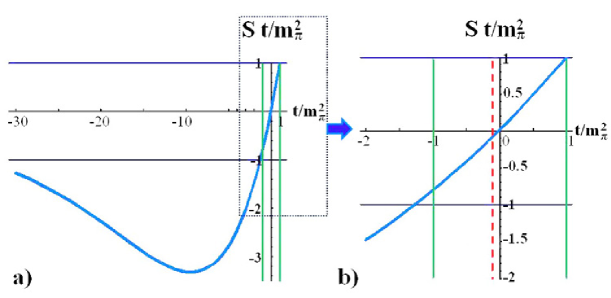
Figure 2: Function from the expression (6) at fixed $\xi=0.05$. The boundary of the physical region $t\simeq-m_{p}^{2}\xi^{2}/(1-\xi)$ is represented by vertical dashed line.

The behavior of corresponding functions is shown in the Fig. 2. When t is equal to mass of the pion squared, we have no absorbtion at all ($S=1$) and extracted cross-sections are independent on the model for rescattering corrections.

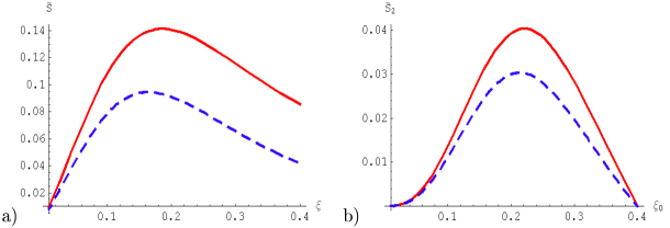
Figure 3: Rescattering corrections integrated with formfactors for $\sqrt{s}=0.9$ TeV (solid) and $\sqrt{s}=7$ TeV (dashed): a) $\tilde{S}(s,\;\xi)$; b) $\tilde{S}_{2}(s,\;\xi_{0})$.

The real situation is more complicated, especially from the experimental point of view. It is rather difficult to measure transverse momentum of a fast leading neutron, we can only get some restrictions on $t$ from the acceptance of detectors. We propose to use the model dependent integrated method presented by formulas

$$\tilde{S}(s,\xi) \!\!\!\!= \!\!\!\!\int_{t_{min}}^{t_{max}}dt\;S\left(\frac{s}{s_{0}},\xi,t\right)F_{\pi}(\xi,t),\;\sigma_{\pi p}\left(M_{\pi p}^{2}\right)=\frac{\frac{d\sigma_{{\rm S}\pi{\rm E}}}{d\xi}}{\tilde{S}(s,\xi)},\;\xi\simeq\frac{M_{\pi p}^{2}}{s},$$ (9)

$$\tilde{S}_{2}(s,\xi_{0}) \!\!\!\!= \!\!\!\!\int_{-y_{0}}^{y_{0}}dy\int_{t_{min}}^{t_{max}}dt_{1}dt_{2}\;S_{2}\left(\frac{s}{s_{0}},\xi_{0}{\rm e}^{\pm y},t_{1,2}\right)F_{\pi}(\xi_{0}{\rm e}^{y},t_{1})F_{\pi}(\xi_{0}{\rm e}^{-y},t_{2}),$$ (10)

$$\sigma_{\pi\pi}\left(M_{\pi\pi}^{2}\right) \!\!\!\!= \!\!\!\!\frac{\frac{d\sigma_{{\rm D}\pi{\rm E}}}{d\xi_{0}}}{\tilde{S}_{2}(s,\xi_{0})},\;\xi_{0}\simeq\frac{M_{\pi\pi}}{\sqrt{s}},\;y_{0}=\ln\frac{\xi_{max}}{\xi_{0}}.$$ (11)

Functions $\tilde{S}$ and $\tilde{S}_{2}$ are shown in the Fig. 3. Models for rescattering give us theoretical errors. If we have the data on p p and anti-p p total and elastic cross-sections, these uncertainties could be reduced to the errors of the data. For example, without LHC measurements at 10 TeV theoretical uncertainties can be estimated only from model predictions and can reach 20% for the most popular models. These errors are low for energies less than 1.9 TeV, since we have precise measurements from Tevatron.

Our method (9) which used a very narrow t interval was applied to the extraction of $\pi^{+}$ p total cross-sections at low energies [1]. It was shown in [1] that extracted points are close to the real data and four different model predictions which is a clear signal of the validity of our method.

3 Pion exchanges with dijet production

Since it is possible to extract $\pi$ p and $\pi$ $\pi$ cross-sections (total, elastic, Drell-Yan, direct photon or inclusive dijet production and so on) from the LHC data it should be possible to use such results to look inside the pion as we usually do it with proton and anti-proton. In this article we consider only the case of the inclusive dijet production as an example.

Let us consider $\pi$ p or $\pi$ $\pi$ scattering with dijet production as a general process of the type $h_{1}+h_{2}\to{\rm jet}\;{\rm jet}\;{\rm X}$ (see Fig. 4 for definitions). Momenta of particles can be represented as usual (for any $p\equiv\{p_{0},p_{3};\;\vec{p}\}$):

$$k_{a} \!\!\!\!= \!\!\!\!\left\{x_{a}p_{h_{1},0},x_{a}p_{h_{1},3};\;\vec{k}_{t,a}\right\},\;k_{b}=\left\{x_{b}p_{h_{2},0},x_{b}p_{h_{2},3};\;\vec{k}_{t,b}\right\},$$ (12)

$$k_{i} \!\!\!\!= \!\!\!\!\left(k_{t,i}\cosh\eta_{i},k_{t,i}\sinh\eta_{i};\;\vec{k}_{t,i}\right),\;i=c,d,$$ (13)

$$\hat{s} \!\!\!\!\simeq \!\!\!\!x_{a}x_{b}M_{h_{1}h_{2}}^{2}\simeq M_{jj}^{2}=(k_{c}+k_{d})^{2}=(k_{a}+k_{b})^{2},$$ (14)

$$\hat{t} \!\!\!\!= \!\!\!\!(k_{a}-k_{c})^{2}=(k_{b}-k_{d})^{2}.$$ (15)

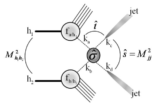
Figure 4: Process $h_{1}+h_{2}\to{\rm jet}\;{\rm jet}\;{\rm X}$.

In the case of $\pi$ p scattering we have

$$p_{h_{1}}=p_{\pi}\simeq\left\{\xi\frac{\sqrt{s}}{2},\xi\frac{\sqrt{s}}{2};\;\vec{q}\right\},\;p_{h_{2}}=p_{2}\simeq\left\{\frac{\sqrt{s}}{2},-\frac{\sqrt{s}}{2};\;\vec{0}\right\}$$

and for $\pi$ $\pi$ scattering

$$p_{h_{1}}=p_{\pi,1}\simeq\left\{\xi_{1}\frac{\sqrt{s}}{2},\xi_{1}\frac{\sqrt{s}}{2};\;\vec{q}_{1}\right\},\;p_{h_{2}}=p_{\pi,2}\simeq\left\{\xi_{2}\frac{\sqrt{s}}{2},-\xi_{2}\frac{\sqrt{s}}{2};\;\vec{q}_{2}\right\}.$$

For $|t_{i}|\ll m_{h_{1},h_{2}}^{2}\ll M^{2}_{h_{1}h_{2}}$ we have

$$x_{a}=\frac{1}{2p_{h_{1},0}}\left(m_{\perp,c}\;{\rm e}^{\eta_{c}}+m_{\perp,d}\;{\rm e}^{\eta_{d}}\right),\;x_{b}=\frac{1}{2p_{h_{2},0}}\left(m_{\perp,c}\;{\rm e}^{-\eta_{c}}+m_{\perp,d}\;{\rm e}^{-\eta_{d}}\right),$$

$$m_{\perp,i}=\sqrt{m_{i}^{2}+k_{t,i}^{2}}.$$ (16)

And in the collinear approximation $k_{t,\;a,b}\ll k_{t}\simeq k_{t,c}\simeq k_{t,d}$, $m_{a,b,c,d}\ll k_{t}$

$$x_{a}=\frac{k_{t}}{p_{h_{1},0}}{\rm e}^{y}\cosh\eta,\;x_{b}=\frac{k_{t}}{p_{h_{2},0}}{\rm e}^{-y}\cosh\eta,$$

$$M_{jj}\simeq 2k_{t}\cosh\eta,\;\eta=\frac{\eta_{d}-\eta_{c}}{2},\;y=\frac{\eta_{d}+\eta_{c}}{2},$$

$$\hat{t}\simeq-\frac{\hat{s}}{2}(1+z),\;\hat{u}\simeq-\frac{\hat{s}}{2}(1-z),\;z=\tanh\eta=\cos\theta^{*},$$ (17)

where $\theta^{*}$ is the scattering angle in the CM frame of partons a and b.

The basic formula for inclusive two parton production in the collinear approximation looks as follows

$$\frac{d\sigma_{h_{1}+h_{2}\to c\;d\;X}(M_{h_{1}h_{2}}^{2})}{dx_{a}dx_{b}dz}=\frac{\hat{s}}{2}\sum_{a,b}f_{a/h_{1}}(x_{a})f_{b/h_{2}}(x_{b})\frac{d\hat{\sigma}_{ab\to cd}}{d\hat{t}}(\hat{s};\;z)=$$

$$=\sum_{a,b}f_{a/h_{1}}(x_{a})f_{b/h_{2}}(x_{b})\frac{d\hat{\sigma}_{ab\to cd}}{dz}(\hat{s};\;z),$$ (18)

where $f_{i/h}(x)$ is the number density of parton $i$ (quark, anti-quark or gluon) with the longitudinal momentum $x\;p_{h,0}$ in the hadron $h$. Renormalization and factorization scales are hidden in $G$ and $\hat{\sigma}$. We can reconstruct momenta of final partons from jets measurements and then use our method (9)-(11) to obtain combinations of PDFs in the pion and a proton. Since we know proton PDFs from other experiments, we can extract combinations of pion’s PDFs

$$\sum_{a,b}f_{a/\pi}(x_{a})\tilde{f}_{b/p}(s\;\xi\;x_{a})=\frac{\frac{d\sigma_{{\rm S}\pi{\rm E}}^{jj}}{d\xi dx_{a}}}{\tilde{S}(s,\xi)},$$ (19)

$$\tilde{f}_{b/p}(s\;\xi\;x_{a})=\int dx_{b}\;f_{b/p}(x_{b})\hat{\sigma}_{ab\to cd}(s\;\xi\;x_{a}x_{b}),$$ (20)

$$\sum_{a,b}f_{a/\pi}(x_{a})f_{b/\pi}(x_{b})\hat{\sigma}_{ab\to cd}(s\;\xi_{0}^{2}x_{a}x_{b})=\frac{\frac{d\sigma_{{\rm D}\pi{\rm E}}^{jj}}{d\xi_{0}dx_{a}dx_{b}}}{\tilde{S}_{2}(s,\xi_{0})},$$ (21)

and $d\hat{\sigma}_{ab\to cd}/dz$ can be found in the Table 1.

Table 1: Leading order parton-parton cross-sections $d\hat{\sigma}_{ab\to cd}/dz=\frac{\pi\alpha_{s}^{2}}{2\hat{s}}A_{ab\to cd}(\hat{s},\hat{t},\hat{u})$.

Subrocess	$A_{ab\to cd}$
$qq^{\prime}\to qq^{\prime}$	$\frac{4}{9}\frac{\hat{s}^{2}+\hat{u}^{2}}{\hat{t}^{2}}$
$qq\to qq$	$\frac{4}{9}\left[\frac{\hat{s}^{2}+\hat{u}^{2}}{\hat{t}^{2}}+\frac{\hat{s}^{2}+\hat{t}^{2}}{\hat{u}^{2}}\right]-\frac{8}{27}\frac{\hat{s}^{2}}{\hat{t}\hat{u}}$
$q\bar{q}\to q^{\prime}\bar{q}^{\prime}$	$\frac{4}{9}\frac{\hat{t}^{2}+\hat{u}^{2}}{\hat{s}^{2}}$
$q\bar{q}\to q\bar{q}$	$\frac{4}{9}\left[\frac{\hat{s}^{2}+\hat{u}^{2}}{\hat{t}^{2}}+\frac{\hat{u}^{2}+\hat{t}^{2}}{\hat{s}^{2}}\right]-\frac{8}{27}\frac{\hat{u}^{2}}{\hat{s}\hat{t}}$
$gq\to gq$	$-\frac{4}{9}\left[\frac{\hat{s}}{\hat{u}}+\frac{\hat{u}}{\hat{s}}\right]+\frac{4}{9}\frac{\hat{s}^{2}+\hat{u}^{2}}{\hat{t}^{2}}$
$q\bar{q}\to gg$	$\frac{32}{27}\left[\frac{\hat{t}}{\hat{u}}+\frac{\hat{u}}{\hat{t}}\right]-\frac{8}{3}\frac{\hat{t}^{2}+\hat{u}^{2}}{\hat{s}^{2}}$
$gg\to q\bar{q}$	$\frac{1}{6}\left[\frac{\hat{t}}{\hat{u}}+\frac{\hat{u}}{\hat{t}}\right]-\frac{3}{8}\frac{\hat{t}^{2}+\hat{u}^{2}}{\hat{s}^{2}}$
$gg\to gg$	$\frac{9}{2}\left[3-\frac{\hat{t}\hat{u}}{\hat{s}^{2}}-\frac{\hat{s}\hat{u}}{\hat{t}^{2}}-\frac{\hat{s}\hat{t}}{\hat{u}^{2}}\right]$

4 Experimental possibilities.

We propose to measure jet production in single and double pion exchange reactions ((1), (2)) at the LHC using the CMS detector [25]. Diagrams of the reactions (1) and (2) are shown on the Fig. 5 (a) and (b) correspondingly.

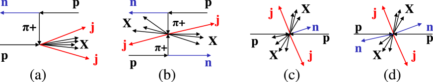
Figure 5: (a) and (b): diagrams for the processes of S$\pi$E and D$\pi$E with 2-jet production. (c) and (d): diagrams for the processes of $pp$ inelastic interactions with 2 jets and leading neutrons production, which can imitate processes (a) and (b).

In these processes two jets are produced in the hard $\pi^{+}p$ and $\pi^{+}\pi^{+}$ scattering which allows us to study parton distributions in pions in a still unexplored kinematical region. In this chapter we discuss perspectives of such measurements at 7 TeV. The Zero Degree Calorimeters (ZDCs) [26] can be used [1, 2] to measure the leading neutrons. The ZDCs are placed on the both sides of CMS, 140m away from the interaction point. They have electromagnetic and hadronic sections designed to measure photons and neutrons in the pseudorapidity region $|\eta|>8.5$.

The Monte-Carlo generator MONCHER v.1.0 [27] has been used for numerical simulation of the processes (1) and (2). This generator is developed by two of the authors of the article for S$\pi$E and D$\pi$E simulation specially. The kinematics of S$\pi$E and D$\pi$E reactions are defined by the relative energy loss $\xi_{n}$ and the square of the transverse momentum $t_{n}$ of the leading neutron. The vertex $p\pi^{+}_{virt}n$ is generated according to the model described in the Ref. [1, 2]. PYTHIA 6.420 [9] is used for the $\pi^{+}_{virt}p\to X$ generation for the single pion exchange and $\pi^{+}_{virt}\pi^{+}_{virt}\to X$ generation for the double pion exchange. All background processes have been generated by PYTHIA 6.420. Diagrams of two background processes, $pp$ inelastic interactions with 2 jets and leading neutrons production imitating signal, are presented on the Fig. 5 (c) and (d).

PYTHIA 6.420 predicts 90.76 mb for the $pp$ total cross section at 7 TeV. The inelastic part of this cross section, which is interesting for us as background, consists of 48.4 mb of minimum bias events, 13.7 mb of single diffractive events and 9.3 mb of double diffractive events. MONCHER 1.0 predicts 1.31$\div$1.85 mb for S$\pi$E and 0.17$\div$0.30 mb for D$\pi$E processes at 7 TeV. Uncertainty in the cross sections comes from the different models for $\pi^{+}p$ and $\pi^{+}\pi^{+}$ interactions. In this study we use the most pessimistic estimations from the Donnachie-Landshoff parametrization [28]. Therefore before any selections the ratio of the signal and background processes at 7 TeV looks as follows:

$$\rm\sigma_{D\pi E}:\sigma_{S\pi E}:\sigma_{TOTAL}=1:7.6:530.$$

In the rest of this paper we seek effective criteria to raise the signal/background ratio for single and double pion exchange.

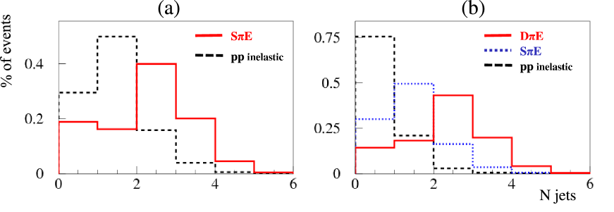
Figure 6: (a) Multiplicity distribution of jets from the S$\pi$E (red(solid)) and $pp$ inelastic events (black(dashed)) selected by (22). (b) Multiplicity distribution of jets from the D$\pi$E (red(solid)), S$\pi$E (blue(dotted)) and $pp$ inelastic events (black(dashed)) selected by (23).

For S$\pi$E we selected events with signal from neutrons in the forward or backward ZDC and with the absence of neutrons in the opposite one:

$$\left[\begin{array}[]{l}\rm N_{n}^{f}>0\quad\&\quad N_{n}^{b}=0\quad\&\quad\xi_{n}^{f}<0.4\\ \rm N_{n}^{b}>0\quad\&\quad N_{n}^{f}=0\quad\&\quad\xi_{n}^{b}<0.4.\end{array}\right.$$ (22)

For the D$\pi$E we selected events with neutrons on both sides:

$$\begin{array}[]{l}\rm N_{n}^{f}>0\quad\&\quad N_{n}^{b}>0\quad\&\quad\xi_{n}^{f}<0.4\quad\&\quad\xi_{n}^{b}<0.4.\end{array}$$ (23)

Here, $N_{n}^{f}$ ($N_{n}^{b}$) is the number of neutrons hitting the forward (backward) ZDC, $\xi_{n}^{f}$ ($\xi_{n}^{b}$) is the relative energy loss of the forward (backward) neutron. The signal to background ratio becomes equal to 0.22 for the S$\pi$E and 0.76 for the D$\pi$E after selections (22) and (23) respectively. For S$\pi$E all background events are produced in the inelastic $pp$ interactions (minimum bias, single and double diffraction). For D$\pi$E 20% of background are imitated by S$\pi$E and 80% come from $pp$ inelastic interactions.

Fig.6 presents distributions of the multiplicity $N^{jets}$ of the jets from S$\pi$E, D$\pi$E and $pp$ inelastic events selected by (22) (a) and by (23) (b). Signal (red solid histograms) and background (blue dotted and black dashed) have rather different distributions of $N^{jets}$. For the analysis we selected 2-jet events dominating in the S$\pi$E and D$\pi$E production(around 40%).

Fig. 7 (a) and (b) shows pseudorapidity distributions in $\eta^{jets}$ and transverse momentum $p_{t}^{jets}$ of jets from the 2-jet S$\pi$E (red(solid)) and $pp$ inelastic (black(dashed)) events selected by (22). The $p_{t}^{jets}$ distribution of the jets from signal (red (solid) histogram) shows a more gentle sloping behaviour comparing with jets from background (black (dashed) histogram). It can be used for the further signal/background separation. Vertical lines on the plot (a) show the total Barrel, Endcap and HF acceptance of CMS. Plot (c) on the Fig. 7 presents the distribution of the sum of jets and neutron energies, $E_{jjn}=E_{j1}+E_{j2}+E_{n}$, for the signal and background 2-jet events selected by (22). The last right bin of the distribution, peaking at 7 TeV, corresponds to the exclusive production of jets. Events with $E_{jjn}<7$ TeV come from the inclusive jets production. It is seen that 2-jet signal events are produced in the exclusive process dominantly (ratio of exclusive to inclusive production is approximately equal to $8.4$). For the background, inversely, inclusive production of 2-jet events is more intensive (exlusive/inclusive ratio is approximately equal to $0.23$). We also use this difference for the further signal/background separation.

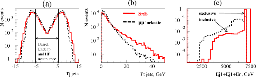
Figure 7: Distributions in $\eta^{jets}$ (a), transverse momentum $p_{t}^{jets}$ (b) of jets and the sum of jets and neutron energies,$E_{jjn}=E_{j1}+E_{j2}+E_{n}$, from the 2-jet S$\pi$E (red(solid)) and $pp$ inelastic events (black(dashed)) selected by (22). The last right bin of the distribution (c), peaking at 7 TeV, corresponds to the exclusive production of jets. Events with $E_{jjn}<7$ TeV on the plot (c) come from the inclusive jets production. Vertical lines on the plot (a) shows Barrel, Endcap and HF acceptance of the CMS.

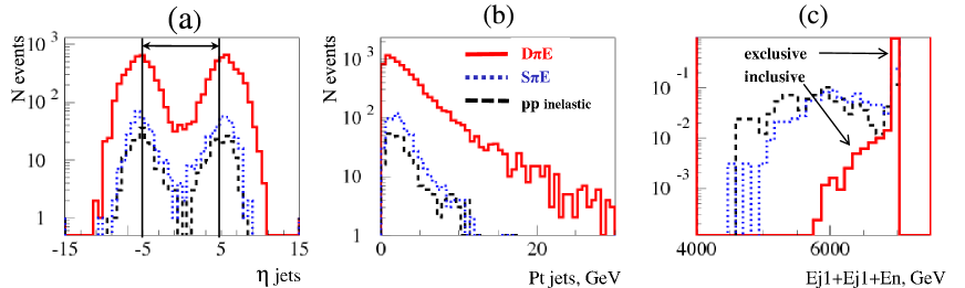
Figure 8: The same as on the Fig.7 for the 2-jet D$\pi$E (red(solid)), S$\pi$E (blue(dotted)) and $pp$ inelastic events (black(dashed)) selected by (23).

Fig. 8 shows the same distributions as Fig. 7 for D$\pi$E (red (solid) histogram), S$\pi$E (blue (dotted)) and $pp$ inelastic (black (dashed)) 2-jet events selected by (23). The difference between signal and background in the $p_{t}^{jets}$ distributions becomes more essential. Practically, there are no background events at $p_{t}^{jets}>10$ GeV, which can be used for the total separation of the 2-jet D$\pi$E events from background. Almost all 2-jet D$\pi$E events selected by (22) are produced exclusively. The ratio of exclusive to inclusive production is equal $\approx 14$.

Analysing distributions of jets for signal and background we suggest the following cuts

$$\left\{\begin{array}[]{l}\rm|\eta^{jets}|<5\\ \rm p_{t}^{jets}>30\ GeV,\\ \end{array}\right.$$ (24)

for 2-jet S$\pi$E events selection and

$$\left\{\begin{array}[]{l}\rm|\eta^{jets}|<5\\ \rm p_{t}^{jets}>10\ GeV,\\ \end{array}\right.$$ (25)

for 2-jet D$\pi$E events selection. $p_{t}^{jets}$-cut can be varied depending on trigger requirements and number of detected events to optimize signal/background ratio.

Events of the reaction (1) selected by (22)&(24) have $\approx$15% of background from 2-jet $pp$ inelastic production with leading neutrons. Events of the reaction (2) selected by (23)&(25) have $\approx$3% of background from $pp$ inelastic and S$\pi$E production imitating signal. The additinal requirement

$$\rm 6990<\sum{(E_{jets}+E_{neutrons})}<7010\ GeV,$$ (26)

selecting events with exclusive jets production, allows to suppress background for (1) down to the level 6.5% and completely suppress the background for (2).

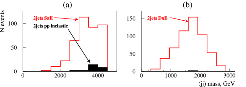
Figure 9: Distributions of events in (a) Invariant mass of (jj) system for S$\pi$E events selected by (22)&(24)&(26) is shown by red (solid) line. 3% of background from $pp$ inelastic events is shown by black histogram. (b) Invariant mass of (jj) system for D$\pi$E events selected by (23)&(25)&(26).

Invariant mass of the 2-jet system produced exclusively in the reaction (1) is shown on the Fig. 9 (a) for the events selected by (22)&(24)&(26). Invariant mass of the 2-jet system produced exclusively in the reaction (2) is shown on the Fig. 9 (b) for the events selected by (23)&(25)&(26). Efficiency of the signal selection depends on $p_{t}^{jets}$-cut dominantly. With selections (22)&(24)&(26) we save 2% of the single pion exchange events (1) and 9% of the double pion exchange events (2) with (23)&(25)&(26).

5 Discussions and conclusions

We propose to measure reactions of single (S$\pi$E) and double (D$\pi$E) pion exchange with 2-jet production at the LHC with CMS [25] using the ZDC calorimeter [26] to detect leading neutrons. Numerical simulation of reactions (1) and (2) has been performed with MONCHER 1.0 [27] event generator. Background events from 2-jet $pp$ inelastic interactions have been generated by PYTHIA 6.420 [9]. In this study we investigated effective criteria for selection of events in reactions (1) and (2) and estimated signal/background ratio. On the generator level of simulation the perspectives for such measurements look quite positive.

For 2-jet D$\pi$E events we can suppress completely the background from S$\pi$E and $pp$ inelastic interactions using a trigger for neutrons from ZDC (selections (23)) and properties of the jets measured in Barrel, Endcap and HF of the CMS (selection (25)). The rest of the 2-jet D$\pi$E events after all selections, 9%, is equivalent to $\approx 8\div 12\mu$b (uncertainty is caused by different predictions for D$\pi$E cross section).

For 2-jet S$\pi$E events we suggested selections (22)&(24)&(26) which use only trigger requirements for neutrons from the ZDC and properties of jets. These selections suppress background from 2-jet inelastic events almost completely and save $\approx 2\%$ of the signal, which is equivalent to $\approx 10\div 14\mu$b.

The data accumulated by the CMS detector (more than 300 pb^-1 at a time of the writing of this text) gives chances to extract millions of pure 2-jet S$\pi$E and D$\pi$E events, which are exclusive dominantly, for the detailed investigation of PDFs in the pion.

From the theoretical point of view it would be very impressive if we had parton distributions in the pion in a still unexplored kinematical region, since pion is a fundamental “participant” of the strong interaction. Also comparison of PDFs in the pion and the proton (anti-proton) can shed light on the mechanism of quark confinement and differences in the internal (quark, gluon) field structure of mesons and baryons.

References

• [1] V. Petrov, R. Ryutin and A. Sobol, LHC as $\pi p$ and $\pi\pi$ collider, Eur. Phys. J. C. 65 (2010) 637.
• [2] A. Sobol, R. Ryutin, V. Petrov, M. Murray, Elastic $\pi^{+}p$ and $\pi^{+}\pi^{+}$ scattering at LHC, Eur. Phys. J. C 69 (2010) 641.
• [3] R.A. Ryutin, V.A. Petrov, A.E. Sobol, Towards extraction of $\pi^{+}\;p$ and $\pi^{+}\pi^{+}$ cross-sections from charge exchange processes at the LHC, arXiv:1101.0078 [hep-ph], Eur. Phys. J. C 71 (2011) 1667.
• [4] http://durpdg.dur.ac.uk/
• [5] M. Dittmar et al., Parton distributions, e-Print: arXiv:0901.2504 [hep-ph].
• [6] C. Weiss, Generalized parton distributions: Status and perspectives, AIP Conf.Proc.1149 (2009) 150.
• [7] A.V. Belitsky, A.V. Radyushkin, Unraveling hadron structure with generalized parton distributions, Phys. Rep. 418 (2005) 1.
• [8] A.D. Martin, W.J. Stirling, R.S. Thorne, G. Watt, Parton distributions for the LHC, Eur. Phys. J. C63 (2009) 189.
• [9] T. Sjostrand, S. Mrenna, P. Skands, PYTHIA 6.4 Physics and Manual, JHEP 0605 (2006) 026.
• [10] By E609 Collaboration (A. Bordner et al.), Experimental information on the pion gluon distribution function, Z. Phys. C72 (1996) 249.
• [11] A.D. Martin., R.G. Roberts., W.J. Stirling and P.J. Sutton, Parton distributions for the pion extracted from Drell-Yan and prompt photon experiments, Phys. Rev. D45 (1992) 2349.
• [12] M. Gluck, E. Reya, I. Schienbein, Pionic parton distributions revisited, Eur. Phys. J. C10 (1999) 313.
• [13] H. Holtmann, G. Levman, N.N. Nikolaev, A. Szczurek, J. Speth, How to measure the pion structure function at HERA, Phys. Lett. B338 (1994) 363.
• [14] G. Levman, The Structure of the pion and nucleon, and leading neutron production at HERA, Nucl. Phys. B642 (2002) 3.
• [15] M. Klasen, The Pion structure function and jet production in gamma $p\to n\;X$, J. Phys. G28 (2002) 1091.
• [16] M. Klasen, G. Kramer, Photoproduction of jets on a virtual pion target in next-to-leading order QCD, Phys. Lett. B508 (2001) 259.
• [17] W. Selove et al., Search for difference in pion / proton internal structure, preprint: FERMILAB-PROPOSAL-0246 (1973).
• [18] V. Stoks, R. Timmermans and J.J. de Swart, On the pion - nucleon coupling constant, Phys. Rev. C 47 (1993) 512; R.A. Arndt, I.I. Strakovsky, R.L. Workman and M.M. Pavan, Updated analysis of $\pi\;N$ elastic scattering data to 2.1-GeV: The Baryon spectrum, Phys. Rev. C 52 (1995) 2120.
• [19] ZEUS Collab., S Chekanov et al., Leading neutron production in $e^{+}\;p$ collisions at HERA, Nucl. Phys. B 637 (2002) 3.
• [20] B.Z. Kopeliovich, B. Povh and I. Potashnikova, Deep inelastic electroproduction of neutrons in the proton fragmentation region, Z. Phys. C 73 (1996) 125.
• [21] K.G. Boreskov, A.B. Kaidalov and L.A. Ponomarev, Nucleon spectra in p p collisions and the reggeized pi-meson exchange model, Sov. J. Nucl. Phys. 19 (1974) 565.
• [22] K.G. Boreskov, A.B. Kaidalov, V.I. Lisin, E.S. Nikolaevskii, L.A. Ponomarev, Model of reggeized one pion exchange and reaction $p\;p\;\to\;p\;n\pi^{+}$, Sov.J.Nucl.Phys. 15 (1972) 203.
• [23] C. Goebel, Determination of the $\pi-\pi$ Interaction Strength from $\pi-N$ Scattering, Phys. Rev. Lett. 1 (1958) 337.
• [24] G.F. Chew and F.E. Low, Unstable particles as targets in scattering experiments, Phys. Rev. 113 (1959) 1640.
• [25] The Compact Muon Solenoid, Technical Proposal, CERN/LHCC-94-38, LHCC/P1.
• [26] A.S. Ayan et. al., ZDC Technical Design Report, CMS-IN-2006/54.
• [27] A. Sobol, R. Ryutin, MonChERv1.0. (Monte-Carlo for CHarge Exchange Reactions), talk presented at the FWD PAG meeting, 29.03.2011, CERN.
• [28] A. Donnachie, P.V. Landshoff, Total cross-sections, Phys. Lett. B 296 (1992) 227.