Large deviations for cluster size distributions in a continuous classical many-body system

Abstract

An interesting problem in statistical physics is the condensation of classical particles in droplets or clusters when the pair-interaction is given by a stable Lennard–Jones-type potential. We study two aspects of this problem. We start by deriving a large deviations principle for the cluster size distribution for any inverse temperature $\beta\in(0,\infty)$ and particle density $\rho\in(0,\rho_{\mathrm{cp}})$ in the thermodynamic limit. Here $\rho_{\mathrm{cp}}>0$ is the close packing density. While in general the rate function is an abstract object, our second main result is the $\Gamma$-convergence of the rate function toward an explicit limiting rate function in the low-temperature dilute limit $\beta\to\infty$, $\rho\downarrow 0$ such that $-\beta^{-1}\log\rho\to\nu$ for some $\nu\in(0,\infty)$. The limiting rate function and its minimisers appeared in recent work, where the temperature and the particle density were coupled with the particle number. In the decoupled limit considered here, we prove that just one cluster size is dominant, depending on the parameter $\nu$. Under additional assumptions on the potential, the $\Gamma$-convergence along curves can be strengthened to uniform bounds, valid in a low-temperature, low-density rectangle.

T1Supported by the DFG-Forschergruppe 718 “Analysis and Stochastics in Complex Physical Systems.”

, and

1 Introduction

We consider interacting $N$-particle systems in a box $\Lambda=[0,L]^{d}\subset\mathbb{R}^{d}$ with interaction energy

$$U_{N}(x_{1},\ldots,x_{N}):=\sum_{1\leq i<j\leq N}v\bigl{(}|x_{i}-x_{j}|\bigr{)},$$ (1)

where $v\dvtx[0,\infty)\to\mathbb{R}\cup\{\infty\}$ is a pair potential of Lennard–Jones type; see Figure 1. That is:

• it is large close to zero, inducing a repulsion that prevents the particles from clumping;

• it has a nondegenerate negative part, inducing an attraction, that is, particles try to assume a certain fixed distance to each other;

• it vanishes at infinity; that is, long-range effects are absent.

Additionally, we always assume that $v$ is stable and has compact support. We allow for the possibility that $v=\infty$ in some interval $[0,r_{\mathrm{hc}}]$ to represent hard core interaction. See Assumption (V) in Section 1.2 below for details.

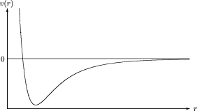
Figure 1: The pair potential $v(r)=1.5r^{-12}-5r^{-6}$ of Lennard–Jones type.

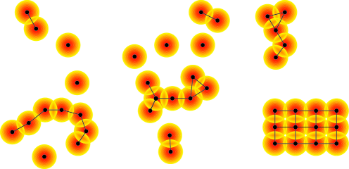
Figure 2: A schematic figure illustrating the cluster decomposition of a particle configuration and the induced graph structure.

A particle configuration $\mathbf{x}=(x_{1},\ldots,x_{N})$ in the box is randomly structured into a number of smaller subconfigurations, that is, well-separated smaller groups, which we call clusters; see Figure 2. One of our main questions is about the joint distribution of the cluster sizes, that is, their cardinalities. Intuitively, if the box size is large in comparison to the particle number, then one expects many small clusters, and if it is small, then one expects few large ones. We will analyse this question more closely in the thermodynamic limit, that is, keeping $\beta\in(0,\infty)$ fixed and taking

$$N\to\infty,L=L_{N}\to\infty\mbox{ such that}\qquad\frac{N}{L_{N}^{d}}\to\rho,$$ (2)

for some fixed particle density $\rho\in(0,\infty)$, followed by the dilute low-temperature limit

$$\beta\to\infty,\rho\downarrow 0\mbox{ such that}\qquad{-}\frac{1}{\beta}\log\rho\to\nu,$$ (3)

for some $\nu\in(0,\infty)$. In this regime, the total entropy of the system is well approximated by the sum of the entropies of the clusters, and the excluded-volume effect between the clusters as well as the mixing entropy may be neglected. As a consequence, particles tend to favor one optimal cluster size, which depends on $\nu$ and may be infinite.

In recent work CKMS10 , the free energy was analysed in the coupled dilute low-temperature limit

$$N\to\infty,\beta=\beta_{N}\to\infty,L=L_{N}\to\infty\mbox{ such that}$$

(4)

$$\qquad-\frac{1}{\beta_{N}}\log\frac{N}{L_{N}^{d}}\to\nu,$$

with some constant $\nu\in(0,\infty)$. It was found that the limiting free energy is a piecewise linear, continuous function of $\nu$ with at least one kink, that is, nondifferentiable point. Furthermore, there was a phenomenological discussion of the interplay between the limiting cluster distribution and the kinks in the limiting free energy, on base of a variational representation. See Section 1.3 for details.

In the present paper, we go beyond CKMS10 by considering the physically relevant setting of a thermodynamic limit and by proving limit laws for the quantities of interest. That is, our two main purposes are: [(ii)]

to derive, for fixed $\beta,\rho\in(0,\infty)$, a large deviations principle for the cluster size distribution in the thermodynamic limit in (2), and

to derive afterwards limit laws (laws of large numbers) for the cluster size distribution in the low-temperature dilute limit in (3). In this way, we decouple the limit in (1) into taking two separate limits, and we prove limit laws for the cluster sizes in this regime.

The organisation of Section 1 is as follows. In Section 1.1 we introduce our model and define the thermodynamic set-up. Our main result concerning the large deviations principle for the cluster size distribution is formulated in Section 1.2. The low-temperature dilute limit is discussed in Sections 1.3 and 1.4. Adopting additional, stronger assumptions we give in Section 1.5 bounds that are uniform in the temperature for dilute systems. Finally we discuss in Section 1.6 some mathematical and physical problems related to our results.

1.1 The model and its thermodynamic set-up

Here are our assumptions on the pair interaction potential that will be in force throughout the paper.

Assumption (V).

The function $v\dvtx[0,\infty)\to\mathbb{R}\cup\{\infty\}$ satisfies the following: [(1)]

$v$ is finite except possibly for a hard core: there is a $r_{\mathrm{hc}}\geq 0$ such that $v\equiv\infty$ on $(0,r_{\mathrm{hc}})$ and $v<\infty$ on $(r_{\mathrm{hc}},\infty)$.

$v$ is stable, that is, $U_{N}(\mathbf{x})/N$ is bounded from below in $N\in\mathbb{N}$ and $\mathbf{x}\in(\mathbb{R}^{d})^{N}$.

The support of $v$ is compact, more precisely, $b:=\sup\operatorname{supp}(v)$ is finite.

$v$ has an attractive tail: there is a $\delta\in(0,b)$ such that $v(r)<0$ for all $r\in(b-\delta,b)$.

$v$ is continuous in $[r_{\mathrm{hc}},\infty)$.

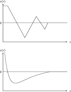
Figure 3: Two examples of pair interaction potentials satisfying Assumption (V).

See Figure 3 for two examples. Assumption (V) differs from Assumption (V) in CKMS10 in two points: here we drop the requirement $v(r_{\mathrm{hc}})=\infty$, and stability was there a consequence of some cumbersome additional assumption.

We introduce the Gibbs measure induced by the energy defined in (1). For $\beta\in(0,\infty)$, $N\in\mathbb{N}$ and a box $\Lambda\subset\mathbb{R}^{d}$, we define the probability measure $\mathbb{P}_{\beta,\Lambda}^{({N})}$ on $\Lambda^{N}$ by the Lebesgue density

$$\mathbb{P}_{\beta,\Lambda}^{({N})}(\mathrm{d}\mathbf{x})=\frac{1}{Z_{\Lambda}(\beta,N)N!}\mathrm{e}^{-\beta U_{N}(\mathbf{x})}\,\mathrm{d}\mathbf{x},\qquad\mathbf{x}\in\Lambda^{N},$$ (5)

where

$$Z_{\Lambda}(\beta,N):=\frac{1}{N!}\int_{\Lambda^{N}}\mathrm{e}^{-\beta U_{N}(\mathbf{x})}\,\mathrm{d}\mathbf{x}$$

is the canonical partition function at inverse temperature $\beta$.

We introduce the notions of connectedness and clusters. Fix $R\in(b,\infty)$. Given $\mathbf{x}=(x_{1},\ldots,x_{N})\in(\mathbb{R}^{d})^{N}$, we introduce on the set $\{x_{1},\ldots,x_{N}\}$ a graph structure by connecting two points if their distance is $\leq\!R$. In this way, the notion of $R$-connectedness is naturally introduced, which we also call just connectedness. The connected components are also called clusters. A cluster of cardinality $k\in\mathbb{N}$ is called a $k$-cluster. By $N_{k}(\mathbf{x})$ we denote the number of $k$-clusters in $\mathbf{x}$, and by

$$\rho_{k,\Lambda}(\mathbf{x}):=\frac{N_{k}(\mathbf{x})}{|\Lambda|}$$

the $k$-cluster density, the number of $k$-clusters per unit volume. We consider the cluster size distribution

$$\bolds{\rho}_{\Lambda}:=(\rho_{k,\Lambda})_{k\in\mathbb{N}}$$ (6)

as an $M_{N/|\Lambda|}$-valued random variable, where

$$M_{\rho}:=\biggl{\{}(\rho_{k})_{k\in\mathbb{N}}\in[0,\infty)^{\mathbb{N}}\Big{|}\sum_{k\in\mathbb{N}}k\rho_{k}\leq\rho\biggr{\}},\qquad\rho\in(0,\infty).$$ (7)

On $M_{\rho}$ we consider the topology of pointwise convergence, in which it is compact. Note that for each finite $N$ and any box $\Lambda\subset\mathbb{R}^{d}$,

$$\sum_{k=1}^{N}k\rho_{k,\Lambda}(\mathbf{x})=\frac{N}{|\Lambda|},\qquad\mathbf{x}\in\Lambda^{N}.$$

However, some mass of $\bolds{\rho}_{\Lambda}$ may be lost in the limit $N\to\infty$ to infinitely large clusters. The distribution of $\bolds{\rho}_{\Lambda}$ under the Gibbs measure $\mathbb{P}_{\beta,\Lambda}^{({N})}$ is the main object of our study.

Introduce the free energy per unit volume as

$$f_{\Lambda}\biggl{(}\beta,{\frac{N}{|\Lambda|}}\biggr{)}:=-\frac{1}{\beta|\Lambda|}\log Z_{\Lambda}(\beta,N).$$

It is known Ru99 that the free energy per unit volume in the thermodynamic limit,

$$f(\beta,\rho):=\mathop{\lim_{N,L\to\infty}}_{N/L^{d}\to\rho}f_{[0,L]^{d}}\biggl{(}\beta,{\frac{N}{L^{d}}}\biggr{)},$$ (8)

exists in $\mathbb{R}$ for all $\rho>0$ when there is no hard core, that is, if $r_{\mathrm{hc}}=0$. When $r_{\mathrm{hc}}>0$, there is a threshold $\rho_{\mathrm{cp}}>0$, the close packing density, such that the limit exists and is finite for $\rho\in(0,\rho_{\mathrm{cp}})$, and is $\infty$ for $\rho>\rho_{\mathrm{cp}}$. Since we are interested in dilute systems, that is, small $\rho$, we will always assume that $\rho\in(0,\rho_{\mathrm{cp}})$.

1.2 Large deviations for cluster distribution under the Gibbs measure

Our first main result is a large deviations principle (LDP) for the cluster size distribution under the Gibbs measure. For the concept of large deviations principles, see the monograph DZ98 .

Theorem 1.1 ((Large deviation principle with convex rate function)).

Fix $\beta\in(0,\infty)$ and $\rho\in(0,\rho_{\mathrm{cp}})$. Then, in the thermodynamic limit $N\to\infty$, $L\to\infty$, $N/L^{d}\to\rho$, the distribution of $\bolds{\rho}_{\Lambda}$ under $\mathbb{P}_{\beta,\Lambda}^{({N})}$ with $\Lambda=[0,L]^{d}$ satisfies a large deviations principle on $M_{\rho+\varepsilon}$ with speed $|\Lambda|=L^{d}$, where $\varepsilon>0$ is such that $N/L^{d}\leq\rho+\varepsilon$. The rate function $J_{\beta,\rho}\dvtx M_{\rho+\varepsilon}\to[0,\infty]$ is convex, and its effective domain $\{J_{\beta,\rho}(\cdot)<\infty\}$ is contained in $M_{\rho}$. For $\rho$ sufficiently small, $\{J_{\beta,\rho}(\cdot)<\infty\}$ is equal to $M_{\rho}$.

If we impose $N/L^{d}\leq\rho$, the theorem also holds with $M_{\rho}$ instead of $M_{\rho+\varepsilon}$.

The proof of Theorem 1.1 is in Section 2. Define $f(\beta,\rho,\cdot)\dvtx M_{\rho}\to[0,\infty]$ through the equality

$$J_{\beta,\rho}(\bolds{\rho})=:\beta\bigl{(}f(\beta,\rho,\bolds{\rho})-f(\beta,\rho)\bigr{)}.$$ (9)

Then the LDP may be rewritten, formally, as

$$\frac{1}{N!}\int_{\Lambda^{N}}\mathrm{e}^{-\beta U_{N}(\mathbf{x})}\mathbh{1}\bigl{\{}\bolds{\rho}_{\Lambda}(\mathbf{x})\approx\bolds{\rho}\bigr{\}}\,\mathrm{d}\mathbf{x}\approx\exp\bigl{(}-\beta|\Lambda|f(\beta,\rho,\bolds{\rho})\bigr{)}.$$

Thus $f(\beta,\rho,\bolds{\rho})$ may be considered as the free energy associated with the cluster size distribution $\bolds{\rho}_{\Lambda}$, thought of as an order parameter. The identity $\inf J_{\beta,\rho}=0$ translates into

$$f(\beta,\rho)=\inf_{M_{\rho}}f(\beta,\rho,\cdot).$$

In words: the (unconstrained) free energy is recovered as infimum of the constrained free energy as the order parameter is varied, a relation in the spirit of Landau theory.

It is a general fact from large deviations theory that an LDP implies tightness. More specifically, the LDP of Theorem 1.1 implies a limit law for the cluster size distribution toward the set of minimisers of the rate function. This is even a law of large numbers if this set is a singleton. Hence, Theorem 1.1 gives us control on the limiting behaviour of the cluster size distribution under the Gibbs measure in the thermodynamic limit. However, in the general context of Theorem 1.1, we cannot offer any formula for the rate function $J_{\beta,\rho}$. We have to restrict ourselves to the low-temperature dilute limit (3). In this setting we obtain explicit asymptotic formulae in Section 1.3 below, and this is our second main result.

1.3 The dilute low-temperature limit of the rate function

In this section, we formulate and comment on our main result about the limiting behaviour of the LDP rate function $J_{\beta,\rho}$ introduced in Theorem 1.1 and of its minimisers in the dilute low-temperature limit in (3). This behaviour is explicitly identified in terms of the ground-state energy of $U_{N}$,

$$E_{N}:=\inf_{\mathbf{x}\in(\mathbb{R}^{d})^{N}}U_{N}(\mathbf{x}),\qquad N\in\mathbb{N}.$$

It can be seen as in the proof of CKMS10 , Lemma 1.1, using subadditivity that the limit

$$e_{\infty}:=\lim_{N\to\infty}\frac{E_{N}}{N}\in(-\infty,0)$$

exists. It lies in the nature of the regime in (3) that it is not the cluster size distribution $\rho_{k}$ that will converge toward an interesting limit (actually, these will vanish), but the term $q_{k}=k\rho_{k}/\rho$, which carries the interpretation of frequency of particles in $k$-clusters. Therefore, let

$$\mathcal{Q}:=\biggl{\{}\mathbf{q}=(q_{k})_{k\in\mathbb{N}}\in[0,1]^{\mathbb{N}}\Big{|}\sum_{k\in\mathbb{N}}q_{k}\leq 1\biggr{\}}$$

and introduce, for $\nu\in(0,\infty)$, the map $g_{\nu}\dvtx\mathcal{Q}\to\mathbb{R}$ defined by

$$g_{\nu}(\mathbf{q}):=\sum_{k\in\mathbb{N}}q_{k}\frac{E_{k}-\nu}{k}+\biggl{(}1-\sum_{k\in\mathbb{N}}q_{k}\biggr{)}e_{\infty}.$$ (10)

Our second main result is the following.

Theorem 1.2 (($\Gamma$-convergence of the rate function)).

Let $\nu\in(0,\infty)$. In the limit $\beta\to\infty$, $\rho\to 0$ such that $-\beta^{-1}\log\rho\to\nu$, the function

$$\mathcal{Q}\to\mathbb{R}\cup\{\infty\},\qquad\mathbf{q}=(q_{k})_{k\in\mathbb{N}}\mapsto\frac{1}{\rho}f\biggl{(}\beta,\rho,\biggl{(}\frac{\rho q_{k}}{k}\biggr{)}_{k\in\mathbb{N}}\biggr{)}$$

$\Gamma$-converges to $g_{\nu}$.

For the notion of $\Gamma$-convergence, see the monograph dMaso . Theorem 1.2 is proved in Section 5.1. The physical intuition is the following: at low density, the particle system can be approximated by an ideal gas of clusters; see hillbook , Chapter 5 or sator . “Ideal” means that we neglect the “excluded volume,” that is, the constraint that clusters have mutual distance $\geq R$. As can be seen from the proof of Lemma 3.1, this means that the rate function $f(\beta,\rho,\cdot)$ is well approximated by the ideal free energy

$$f^{\mathrm{ideal}}\bigl{(}\beta,\rho,(\rho_{k})_{k}\bigr{)} := \sum_{k\in\mathbb{N}}k\rho_{k}f_{k}^{\mathrm{cl}}(\beta)+\biggl{(}\rho-\sum_{k\in\mathbb{N}}k\rho_{k}\biggr{)}f_{\infty}^{\mathrm{cl}}(\beta)$$

$${}+\frac{1}{\beta}\sum_{k\in\mathbb{N}}\rho_{k}(\log\rho_{k}-1).$$

Here $f_{k}^{\mathrm{cl}}(\beta)$ and $f_{\infty}^{\mathrm{cl}}(\beta)$ should be thought of as free energies per particle in clusters of size $k$ (resp., in infinitely large clusters); see Section 3 for the precise definitions. The functional $\rho g_{\nu}$ is obtained from $f^{\mathrm{ideal}}$ by two simplifications, justified at low temperatures.

• First, we approximate cluster internal free energies by their ground state energies.

• Second, we split the entropic term as

  $$\frac{1}{\beta}\sum_{k\in\mathbb{N}}\rho_{k}(\log\rho_{k}-1)=\sum_{k\in\mathbb{N}}\rho_{k}\frac{\log\rho}{\beta}+\frac{1}{\beta}\sum_{k\in\mathbb{N}}\rho_{k}\biggl{(}\log\frac{\rho_{k}}{\rho}-1\biggr{)}$$

  and keep only the first sum. Thus we keep the entropic contribution coming from the ways to place the clusters (their centers of gravity) in the box and discard the mixing entropy.

Since these two simplifications suppress physical intuition to some extent, it appears natural to further analyse the consequences of the approximation with the above ideal free energy; this is carried out in JK . Interesting connections with well-known cluster expansions are discussed in J .

In classical statistical physics, the approach we take here goes under the name of a geometric, or droplet, picture of condensation hillbook , sator . This is closely related to the well-known contour picture of the Ising model and lattice gases Ru99 . Lattice gas cluster sizes have been studied, for example, in lebowitz , continuous systems were investigated in murmann , zessin . The focus of these works was on parameter regions where only small clusters occur. Our declared goal, in contrast, is to derive bounds that cover both the small cluster and the large cluster regimes (in the notation introduced below, this means both $\nu>\nu^{*}$ and $\nu<\nu^{*}$).

Under additional assumptions on the pair potential, we can replace the somewhat abstract $\Gamma$-convergence result with more concrete uniform error bounds; see equations (15) to (18) in Theorem 1.8.

The rate function $g_{\nu}$ appeared in CKMS10 in the description of the behaviour of the partition function $Z_{\beta,\Lambda}^{({N})}$ in the coupled dilute low-temperature limit in (1). More precisely, it was shown there that, in this limit, for any $\nu\in(0,\infty)$,

$$-\frac{1}{N\beta_{N}}\log Z_{\beta_{N},\Lambda_{N}}^{({N})}\to\mu(\nu).$$

It was phenemenologically discussed, but it was not given mathematical substance to, the conjecture that the random variable $\mathbf{q}_{\Lambda_{N}}=(k\rho_{k,\Lambda_{N}}/\rho)_{k\in\mathbb{N}}$ under $\mathbb{P}_{\beta_{N},\Lambda_{N}}^{({N})}$ with $\Lambda_{N}=[0,L_{N}]^{d}$ satisfies an LDP with speed $N\beta_{N}$ and rate function given by $g_{\nu}(\cdot)-\mu(\nu)$. This would be in line with Theorems 1.1 and 1.2, and we do believe that this is indeed true, but we make no attempt to prove this.

1.4 Limit laws in the dilute low-temperature limit

The minimiser(s) of the rate function $f(\beta,\rho,\cdot)$ are of high interest, since they describe the limiting behaviour of the cluster size distribution under the Gibbs measure. It is a general fact from the theory of $\Gamma$-limits that $\Gamma$-convergence implies the convergence of minima over compact subsets and of the minimiser(s). For the limiting rate function $g_{\nu}$, the global minimiser has been identified in CKMS10 . The minimum is

$$\mu(\nu)=\inf_{\mathcal{Q}}g_{\nu}=\inf_{N\in\mathbb{N}}\frac{E_{N}-\nu}{N},$$ (12)

and the minimisers are given as follows.

Lemma 1.3 ((Minimisers of $g_{\nu}$)).

The number $\nu^{*}:=\inf_{N\in\mathbb{N}}(E_{N}-Ne_{\infty})$ is strictly positive. The map $\nu\mapsto\mu(\nu)$ is continuous, piecewise affine and concave. Let $\mathcal{N}\subset(0,\infty)$ be the set of points where $\mu(\cdot)$ changes its slope. Then ${\mathcal{N}}$ is bounded, and $\mu(\nu)=-\nu$ for $\nu>\max{\mathcal{N}}$ and $\mu(\nu)=e_{\infty}$ for $\nu<\nu^{*}$. Furthermore:

[(1)]

$\nu^{*}\in\mathcal{N}\subset[\nu^{*},\infty)$, and $\mathcal{N}$ is at most countable with $\nu^{*}$ as only possible accumulation point.

For $\nu>\nu^{*}$, we have $\mu(\nu)<e_{\infty}$ and every minimiser $\mathbf{q}=(q_{k})_{k}$ of $g_{\nu}$ satisfies $\sum_{k\in\mathbb{N}}q_{k}=1$. If $\nu\notin\mathcal{N}$, then $g_{\nu}$ has the unique minimiser $\mathbf{q}^{({\nu})}=(q_{k}^{({\nu})})_{k}$ with $q_{k}^{({\nu})}=\delta_{k,k(\nu)}$ with $k(\nu)$ the unique minimiser of $k\mapsto(E_{k}-\nu)/k$ over $\mathbb{N}$. The map $\nu\mapsto k(\nu)$ is constant between subsequent points in ${\mathcal{N}}$.

For $\nu<\nu^{*}$, we have $\mu(\nu)=e_{\infty}$ and the unique minimiser of $g_{\nu}$ is the constant zero sequence $(q_{k})_{k\in\mathbb{N}}$ with $q_{k}=0$ for any $k$.

This is essentially CKMS10 , Theorem 1.5; the proof is found in the Appendix. If, as in CKMS10 , the point $\infty$ is added to the state space $\mathbb{N}$ of the measures in $\mathcal{Q}$, then the minimisers of $g_{\nu}$ are concentrated on $\mathbb{N}$ for $\nu>\nu^{*}$ and on $\{\infty\}$ for $\nu<\nu^{*}$; it was left open in CKMS10 whether or not the latter regime is nonvoid.

The set $\mathcal{N}$ is infinite if and only if $(E_{k}-ke_{\infty})_{k\in\mathbb{N}}$ has no minimiser. In dimensions $d\geq 2$, it is expected (and shown in some cases; see R81 , yeung ) that $E_{k}-ke_{\infty}\geq\operatorname{cst.}k^{1-1/d}\to\infty$, ensuring that $\mathcal{N}$ is a finite set.

Now we can draw a conclusion from Theorem 1.2 about the limiting behaviour of the minimisers of the rate function in the dilute low-temperature limit. The following assertions are well known consequences from the $\Gamma$-convergence of Theorem 1.2; see dMaso , Theorem 7.4 and Corollary 7.24.

Corollary 1.4.

In the situation of Theorem 1.2: [(1)]

the free energy per particle converges to $\mu(\nu)$,

$$\frac{1}{\rho}f(\beta,\rho)\to\mu(\nu);$$

if $\mu(\cdot)$ is differentiable at $\nu$ [i.e., for $\nu\in(0,\infty)\setminus{\mathcal{N}}$], any minimiser $\bolds{\rho}^{({\beta,\rho})}=(\rho_{k}^{({\beta,\rho})})_{k}$ of $J_{\beta,\rho}$ converges to the minimiser of $g_{\nu}$:

$$\frac{k\rho_{k}^{({\beta,\rho})}}{\rho}\to q_{k}^{({\nu})},\qquad k\in\mathbb{N}.$$

Figure 4: A diagram illustrating the expected relationship of the slope condition $-T\log\rho=-\beta^{-1}\log\rho\to\nu$ and the minimisers of the rate function in the dilute low-temperature limit. The phases I and IV always exist. Depending on the pair potential, there can be values of $\nu$ for which $2\leq k(\nu)<\infty$, yielding intermediate phases (e.g., II and III, although the precise number of intermediate phases will depend on the pair potential).

For an illustration, see Figure 4. Another important consequence of Theorem 1.2, together with the LDP of Theorem 1.1, is a kind of law of large numbers for the cluster size distribution $\bolds{\rho}_{\Lambda_{N}}$ in the thermodynamic limit, followed by the low-temperature dilute limit. A convenient formulation is in terms of the vector $\mathbf{q}_{\Lambda}=(q_{k,\Lambda})_{k\in\mathbb{N}}$ with $q_{k,\Lambda}=k\rho_{k,\Lambda}/\rho$, the frequency of particles in $k$-clusters, if $|\Lambda|=N/\rho$.

Corollary 1.5.

For any $\nu\in(0,\infty)\setminus{\mathcal{N}}$, any $K\in\mathbb{N}$ and any $\varepsilon>0$, if $\beta$ is sufficiently large, $\rho$ sufficiently small and $-\frac{1}{\beta}\log\rho$ is sufficiently close to $\nu$, then, for boxes $\Lambda_{N}$ with volume $N/\rho$,

$$\lim_{N\to\infty}\mathbb{P}_{\beta,\Lambda_{N}}^{({N})}\bigl{(}|q_{k(\nu),\Lambda_{N}}-1|\geq\varepsilon\bigr{)}=0\qquad\mbox{if }\nu>\nu^{*}$$ (13)

and

$$\lim_{N\to\infty}\mathbb{P}_{\beta,\Lambda_{N}}^{({N})}\Biggl{(}\sum_{k=1}^{K}q_{k,\Lambda_{N}}\geq\varepsilon\Biggr{)}=0\qquad\mbox{if }\nu<\nu^{*}.$$ (14)

We prove (13) and (14) simultaneously. Consider the set

$$A=\cases{\displaystyle\biggl{\{}\bolds{\rho}\in M_{\rho}\dvtx\biggl{|}\frac{k(\nu)\rho_{k(\nu)}}{\rho}-1\biggr{|}\geq\varepsilon\biggr{\}},&\quad$\mbox{for }\nu>\nu^{*},$\vspace*{2pt}\cr\displaystyle\Biggl{\{}\bolds{\rho}\in M_{\rho}\dvtx\sum_{k=1}^{K}\frac{k\rho_{k,\Lambda}}{\rho}\geq\varepsilon\Biggr{\}},&\quad$\mbox{for }\nu<\nu^{*}$.}$$

Then the $\Gamma$-convergence of Theorem 1.2 implies dMaso , Theorem 7.4, that

$$\liminf_{\beta,\rho}\frac{1}{\rho}\inf_{A}f(\beta,\rho,\cdot)\geq-\inf_{A}g_{\nu},$$

where $\liminf_{\beta,\rho}$ refers to the limit in Theorem 1.2. Furthermore, it is easy to see from Lemma 1.3 that $\delta=\inf_{A}g_{\nu}-\inf g_{\nu}$ is positive. We pick now $\beta$ so large and $\rho$ so small and $-\beta^{-1}\log\rho$ so close to $\nu$ that $\frac{1}{\rho}\inf_{A}f(\beta,\rho,\cdot)-\inf_{A}g_{\nu}\geq-\delta/4$ and $\frac{1}{\rho}f(\beta,\rho)-\mu(\nu)\leq\delta/4$ [the latter is possible by Corollary 1.4(1)]. Now the LDP of Theorem 1.1 yields that

$$\limsup_{N\to\infty}\frac{1}{|\Lambda_{N}|}\log\mathbb{P}_{\beta,\Lambda_{N}}^{({N})}(\bolds{\rho}_{\Lambda_{N}}\in A)$$

$$\qquad\leq-\inf_{A}I_{\beta,\rho}=-\beta\Bigl{[}\inf_{A}f(\beta,\rho,\cdot)-f(\beta,\rho)\Bigr{]}$$

$$\qquad\leq-\beta\rho\biggl{[}\inf_{A}g_{\nu}-\mu(\nu)-\frac{\delta}{4}-\frac{\delta}{4}\biggr{]}=-\beta\rho\delta/2<0.$$

Hence, $\lim_{N\to\infty}\mathbb{P}_{\beta,\Lambda_{N}}^{({N})}(\bolds{\rho}_{\Lambda_{N}}\in A)=0$. Noting that this probability is identical to the two probabilities on the left of (13) and (14) for our two choices of $A$, finishes the proof.

It may come as a surprise that, for most values of the parameter $\nu$, the cluster size distribution is asymptotically concentrated on just one particular cluster size that depends only on $\nu$. This may be vaguely explained by the fact that the zero-temperature limit $\beta\to\infty$ forces the system to become asymptotically “frozen” in a state in which every cluster size assumes the globally optimal configuration size, which is unique for $\nu\in(\nu^{*},\infty)\setminus{\mathcal{N}}$. Furthermore, note that Corollary 1.5 does not give the existence of “infinite large” clusters (i.e., clusters whose size diverges with $N$) for any value of $\beta$ and $\rho$, not even for $\nu<\nu^{*}$ and $-\beta^{-1}\log\rho\approx\nu$.

1.5 Uniform bounds

Under some natural additional assumptions on the pair potential, the assertions of Theorem 1.2 can be strengthened; see Theorem 1.8 below. Indeed, we will assume that the ground states of the functional $U_{N}$ consist of well-separated particles, which are contained in a ball with volume of order $N$, and we assume some more regularity of the interaction function $v$. Then we show that the $\Gamma$-convergence in Theorem 1.2 in the coupled limit in (3) can be strengthened to estimates that are uniform in some low-temperature, low-density rectangle $(\overline{\beta},\infty)\times(0,\overline{\rho})$. This leads to corresponding uniform estimates on $|\frac{1}{\rho}f(\beta,\rho)-\mu(\nu)|$ and on minimisers. We now formulate this.

Assumption 1.6 ((Minimum interparticle distance, Hölder continuity)).

[(ii)]

There is $r_{\mathrm{min}}\geq r_{\mathrm{hc}}$ such that, for all $N\in\mathbb{N}$, every minimiser $(x_{1},\ldots,\break x_{N})\in(\mathbb{R}^{d})^{N}$ of the energy function $U_{N}$ has interparticle distance lower bounded as $|x_{i}-x_{j}|\geq r_{\mathrm{min}}$, $i\neq j$.

The pair potential $v$ is uniformly Hölder continuous in $[r_{\mathrm{min}},\infty)$.

The existence of a uniform lower bound $r_{\mathrm{min}}$ for ground state interparticle distance is, of course, trivial when the potential has a hard core $r_{\mathrm{hc}}>0$. A sufficient condition for the existence of $r_{\mathrm{min}}>0$ for a potential without hard core is, for example, that $v(r)/r^{d}\to\infty$ as $r\to 0$, as can be shown along Th06 , Lemma 2.2.

Assumption 1.7 ((Maximum interparticle distance)).

There is a constant $c>0$ such that for all $N\in\mathbb{N}$ every minimiser $(x_{1},\ldots,x_{N})\in(\mathbb{R}^{d})^{N}$ of the energy function $U_{N}$ has interparticle distance upper bounded by $|x_{i}-x_{j}|\leq cN^{1/d}$.

On physical grounds, we would expect that this assumption is true for every reasonable potential. To the best of our knowledge, however, nontrivial rigorous results are available in dimension two only, for Radin’s soft disk potential R81 and for potentials satisfying conditions (H1) to (H3) from yeung . These potentials satisfy Assumption 1.6 as well.

Theorem 1.8.

Suppose that in addition to Assumption (V) the pair potential also satisfies Assumptions 1.6 and 1.7. Then there are $\overline{\rho},\overline{\beta},C>0$ such that for every $(\beta,\rho)\in[\overline{\beta},\infty)\times(0,\overline{\rho}]$, putting $\nu:=-\beta^{-1}\log\rho$, the following holds: [(1)]

Estimate on the rate function:

$$\qquad\biggl{|}\frac{1}{\rho}f\biggl{(}\beta,\rho,\biggl{(}{\frac{\rho q_{k}}{k}\biggr{)}_{k\in\mathbb{N}}}\biggr{)}-g_{\nu}\bigl{(}(q_{k})_{k}\bigr{)}\biggr{|}\leq\frac{C}{\beta}\log\beta,\qquad(q_{k})_{k\in\mathbb{N}}\in\mathcal{Q}.$$ (15)

Estimate on the free energy:

$$\biggl{|}\frac{1}{\rho}f(\beta,\rho)-\mu(\nu)\biggr{|}\leq 2\frac{C}{\beta}\log\beta.$$ (16)

Minimisers: For any minimiser $\bolds{\rho}^{({\beta,\rho})}$ of $f(\beta,\rho,\cdot)$, put $\mathbf{q}^{({\beta,\rho})}:=\break(k\rho_{k}^{({\beta,\rho})}/\rho)_{k\in\mathbb{N}}$. Then, if $\nu<\nu^{*}$,

$$\sum_{k\in\mathbb{N}}\frac{q_{k}^{({\beta,\rho})}}{k}\leq 2\frac{C}{\nu^{*}-\nu}\frac{1}{\beta}\log\beta.$$ (17)

If $\nu>\nu^{*}$, then

$$\sum_{k\in M(\nu)}q^{({\beta,\rho})}_{k}\geq 1-2\frac{C}{\Delta(\nu)}\frac{1}{\beta}\log\beta,$$ (18)

where

$$\Delta(\nu):=\inf\biggl{\{}\frac{E_{k}-\nu}{k}\Big{|}k\in\mathbb{N}\setminus M(\nu)\biggr{\}}-\mu(\nu)>0$$

is the gap above the minimum, and $M(\nu)\subset\mathbb{N}$ is the set of minimisers of $((E_{k}-\nu)/k)_{k\in\mathbb{N}}$ [thus $M(\nu)=\{k(\nu)\}$ for $\nu\notin\mathcal{N}$].

Theorem 1.8 is proved in Section 5.2. One can see from the proof that one can choose $\overline{\rho}=(2\alpha+2R)^{-d}$. It follows in particular that the $\Gamma$-convergence and the two convergences from Corollary 1.4 can be strengthened to convergence for just taking $\beta\to\infty$, uniformly in $\rho\in(0,\overline{\rho}]$, with an error of order $\beta^{-1}\log\beta$. This form of the error order term is an artefact of the assumption of Hölder continuity; the constant $C$ depends on the Hölder parameter.

Note that (17) implies that, in the case $\nu<\nu^{*}$, for every $K\in\mathbb{N}$, the fraction of particles in clusters of size $\leq K$ is bounded by

$$\sum_{k\leq K}\frac{k\rho_{k}^{({\beta,\rho})}}{\rho}=\sum_{k\leq K}q_{k}^{({\beta,\rho})}\leq\frac{2C}{\nu^{*}-\nu}K\frac{1}{\beta}\log\beta.$$

This shows that, as $\beta\to\infty$, for some choices of $K=K_{\beta}\to\infty$, the fraction of particles in clusters of size $\leq K_{\beta}$ vanishes; that is, the average cluster size becomes very large. Note that the law of large numbers in (14) in Corollary 1.5 may, under Assumptions 1.6 and 1.7, be proved also with $K$ replaced by $K_{\beta}$.

1.6 Some remarks concerning related mathematical and physical problems

Our problem is connected with continuum percolation problems for interacting particle systems; see the review ghm01 . In our setting of finite systems, the term “percolation” should be replaced with “formation of unbounded components,” that is, clusters whose size diverges as the number of particles goes go infinity. The problem of percolation or nonpercolation for continuous particle systems in an infinite-volume Gibbs state (i.e., in a grand-canonical setting) is studied in pechersky , where Pechersky and Yambartsev prove that, for sufficiently high chemical potential and sufficiently low temperature, percolation does occur. However, they do not give any information on the densities at which percolation occurs. This hinders the physical interpretation, since one cannot say whether the percolation is due to high density or strong attraction. In this light, our results are stronger and at the same time weaker: we do show that a transition from bounded to unbounded clusters happens at low density, but only in a limiting sense along low-temperature, low-density curves; there is no fixed temperature or density at which we prove the formation of unbounded clusters.

In addition, our work has an interesting relationship to quantum Coulomb systems. In the simplest case, a gas of protons and electrons, we may ask whether we observe a fully ionized gas, where protons and electrons stay for themselves, or a gas of neutral molecules, with protons and electrons paired up together. The mathematical model is in terms of a quantum mechanical Hamiltonian in a fermionic Hilbert space for particles of positive and negative charge interacting via a long ranged Coulomb potential. The analogues of our ground states $E_{k}$ are defined as ground state energies of the Hamiltonian restricted to sectors with prescribed particle numbers and center of mass motion removed. Rigorous mathematical results were given by Fefferman fefferman (see also cly ), in the Saha regime, also called atomic or molecular limit: when the temperature goes to $0$ at fixed, negative enough chemical potential, the Coulomb gas behaves like an ideal gas of different types of molecules or particles. The chemical composition is determined by the chemical potential by an energy minimization problem, akin to minimizing $E_{k}-k\mu$ as a function of $k$, which in turn is the grand-canonical version of our auxiliary variational problem $(E_{k}-\nu)/k=\mathrm{min}$.

Our results adapt this quantum Coulomb system picture to a classical setting. From this point of view, the key novelty is that we work in the canonical rather than the grand-canonical ensemble; this allows us to extend results to the region where formation of large clusters occurs. Indeed, in the canonical ensemble we can take the density larger than the transition density, which is conjectured to exist and to be of the order $\exp(-\beta\nu^{*})$, and at the same time impose that the density be small. In the grand-canonical ensemble, we may of course take the chemical potential larger than the transition potential, but then we lose control over the density and cannot apply the dilute mixture approximation.

The remainder of this paper is organised as follows. In Section 2 we prove the LDP of Theorem 1.1, in Section 3 we compare the rate function with an explicit ideal rate function, and in Section 4 we compare temperature-depending quantities with the ground states. Finally, the proofs of Theorems 1.2 and 1.8 are given in Section 5.

2 Proof of the LDP

In this section, we prove Theorem 1.1. We fix $\beta\in(0,\infty)$ and $\rho\in(0,\rho_{\mathrm{cp}})$ throughout this section. In Section 2.1 we explain our strategy and formulate the main steps, and in Sections 2.2–2.4 we prove these steps. The proof of Theorem 1.1 is finished in Section 2.5.

2.1 Strategy

The main idea is to derive first a large deviations principle for the distribution of $(\rho_{k,\Lambda})_{k=1,\ldots,j}$ for fixed $j\in\mathbb{N}$, that is, for the projection of $\bolds{\rho}_{\Lambda}$ on the first $j$ components, and apply the Dawson–Gärtner theorem for the transition to the projective limit as $j\to\infty$. From the proof of the principle for the projection, we isolate an important step (see Proposition 2.1): using standard subadditivity arguments, we prove the existence of thermodynamic limit for constrained free energy, the constraint referring to cluster size concentrations of size $\leq j$. The principle for the projection of $\bolds{\rho}_{\Lambda}$ appears in Proposition 2.2.

Given $N,N_{1},\ldots,N_{j}\in\mathbb{N}_{0}$ define the constrained partition function with fixed cluster numbers of size $\leq j$,

$$\qquad Z_{\Lambda}(\beta,N,N_{1},\ldots,N_{j}):=\frac{1}{N!}\int_{\Lambda^{N}}\mathrm{e}^{-\beta U_{N}(\mathbf{x})}\prod_{k=1}^{j}\mathbh{1}\bigl{\{}N_{k}(\mathbf{x})=N_{k}\bigr{\}}\,\mathrm{d}\mathbf{x}.$$ (19)

Note that $Z_{\Lambda}(\beta,N,N_{1},\ldots,N_{j})=0$ if $\sum_{k=1}^{j}kN_{k}>N$.

In the following we shall often be interested in the interior or boundary of subsets $A\subset[0,\infty)^{j+1}$ for some $j\in\mathbb{N}$. Unless explicitly stated otherwise, $\operatorname{Int}A$ and $\partial A$ refer to the interior and boundary of $A$ considered as a subset of $\mathbb{R}^{j+1}$. In particular, if $0\in A$, then $0$ is automatically a boundary point.

We denote by $\operatorname{dom}h=\{x\dvtx h(x)<\infty\}=\{h(\cdot)<\infty\}$ the effective domain of an $(-\infty,\infty]$-valued function $h$.

Proposition 2.1.

Fix $j\in\mathbb{N}$. Then there is a function $f_{j}(\beta,\cdot)\dvtx\break[0,\infty)^{j+1}\to\mathbb{R}\cup\{\infty\}$ such that:

• $f_{j}(\beta,\cdot)$ is convex and lower semi-continuous;

• its effective domain has nonempty interior $\Delta_{j}:=\operatorname{Int}_{\mathbb{R}^{j+1}}\operatorname{dom}f_{j}(\beta,\cdot)$ and $f_{j}(\beta,\cdot)$ is continuous in $\Delta_{j}$;

• its effective domain is contained in

  $$\operatorname{dom}f_{j}(\beta,\cdot)\subset\overline{\Delta}_{j}\subset\Biggl{\{}(\rho,\rho_{1},\ldots,\rho_{j})\in[0,\infty)^{j+1}\Big{|}\rho\in[0,\rho_{\mathrm{cp}}],\sum_{k=1}^{j}k\rho_{k}\leq\rho\Biggr{\}},$$

and, moreover, if $|\Lambda_{N}|,N,N_{1}^{({N})},\ldots,N_{j}^{({N})}\to\infty$ in such a way that

$$\frac{N}{|\Lambda_{N}|}\to\rho,\frac{N_{1}^{({N})}}{|\Lambda_{N}|}\to\rho_{1},\ldots,\frac{N^{({N})}_{j}}{|\Lambda_{N}|}\to\rho_{j},$$ (20)

then:

• if $(\rho,\rho_{1},\ldots,\rho_{j})\in\Delta_{j}$,

  $$\lim_{N\to\infty}\frac{1}{|\Lambda_{N}|}\log Z_{\Lambda_{N}}\bigl{(}\beta,N,N_{1}^{({N})},\ldots,N_{j}^{({N})}\bigr{)}=-\beta f_{j}(\beta,\rho,\rho_{1},\ldots,\rho_{j}),$$ (21)

  and the limit is finite;

• if $(\rho,\rho_{1},\ldots,\rho_{j})\in\partial\Delta_{j}$ (boundary of $\Delta_{j}$), then

  $$\limsup_{N\to\infty}\frac{1}{|\Lambda_{N}|}\log Z_{\Lambda_{N}}\bigl{(}\beta,N,N_{1}^{({N})},\ldots,N_{j}^{({N})}\bigr{)} \leq -\beta f_{j}(\beta,\rho,\rho_{1},\ldots,\rho_{j})$$

  $$\in \mathbb{R}\cup\{-\infty\};$$

• if $(\rho,\rho_{1},\ldots,\rho_{j})\in\overline{\Delta}_{j}^{\mathrm{c}}$, then (21) holds true, and the limit is $-\beta f_{j}(\beta,\rho,\rho_{1},\break\ldots,\rho_{j})=-\infty$.

This proposition is proved in Section 2.2.

The set $\Delta_{1}$ is related to close-packing situations. For example, when $j=1$ and the density $\rho$ is higher than $1/|B(0,R)|$ (where we recall that $R$ is the parameter in our notion of connectedness), it is impossible to have a gas formed only of $1$-clusters, and we have $f_{1}(\beta,\rho,\rho)=\infty$.

Analogously to (9), let

$$I_{\beta,\rho,j}(\rho_{1},\ldots,\rho_{j}):=\beta\bigl{(}f_{j}(\beta,\rho,\rho_{1},\ldots,\rho_{j})-f(\beta,\rho)\bigr{)}.$$

We will prove in Section 2.4 the following.

Proposition 2.2 ((LDP for projection of $\bolds{\rho}_{\Lambda}$)).

Fix $j\in\mathbb{N}$. Then, in the thermodynamic limit $N\to\infty$, $L\to\infty$, $N/L^{d}\to\rho$, the distribution of $(\rho_{1,\Lambda},\ldots,\rho_{j,\Lambda})$ under the Gibbs measure $\mathbb{P}_{\beta,\Lambda}^{({N})}$ with $\Lambda=[0,L]^{d}$ satisfies a large deviations principle with scale $|\Lambda|$ and rate function $I_{\beta,\rho,j}$. Moreover, the rate function is good and convex.

Recall that a rate function is called good if its level sets are compact. In this case, it is in particular lower semicontinuous. The large deviations principle means that, for any open set ${\mathcal{O}}\subset[0,\infty)^{j}$ and any closed set ${\mathcal{C}}\subset[0,\infty)^{j}$, with $\Lambda=[0,L]^{d}$,

$$\liminf_{N,L\to\infty,N/L^{d}\to\rho}\frac{1}{|\Lambda|}\log\mathbb{P}_{\beta,\Lambda}^{({N})}\bigl{(}(\rho_{1,\Lambda},\ldots,\rho_{j,\Lambda})\in{\mathcal{O}}\bigr{)} \geq -\inf_{{\mathcal{O}}}I_{\beta,\rho,j},$$ (23)

$$\limsup_{N,L\to\infty,N/L^{d}\to\rho}\frac{1}{|\Lambda|}\log\mathbb{P}_{\beta,\Lambda}^{({N})}\bigl{(}(\rho_{1,\Lambda},\ldots,\rho_{j,\Lambda})\in{\mathcal{C}}\bigr{)} \leq -\inf_{{\mathcal{C}}}I_{\beta,\rho,j}.$$ (24)

We refer to (23) as to the lower bound for open sets and to (24) as to the upper bound for closed sets.

2.2 Proof of Proposition 2.1: Subadditivity arguments

In this section we prove Proposition 2.1. For the remainder of this section, we fix $j\in\mathbb{N}$.

The crucial point is the following supermultiplicativity of partition functions, which translates into subadditivity of free energies: Let $N^{\prime},N^{\prime\prime}\in\mathbb{N}$. Let $\Lambda^{\prime},\Lambda^{\prime\prime}$ be two disjoint measurable sets which have mutual distance larger than the potential range $b$, and $\Lambda$ large enough to contain the union of the two. Then

$$Z_{\Lambda}\bigl{(}\beta,N^{\prime}+N^{\prime\prime}\bigr{)}\geq Z_{\Lambda^{\prime}\dot{\cup}\Lambda^{\prime\prime}}\bigl{(}\beta,N^{\prime}+N^{\prime\prime}\bigr{)}\geq Z_{\Lambda^{\prime}}\bigl{(}\beta,N^{\prime}\bigr{)}Z_{\Lambda^{\prime\prime}}\bigl{(}\beta,N^{\prime\prime}\bigr{)}.$$ (25)

This standard trick leads to a proof of the existence of the thermodynamic limit by subadditivity methods Ru99 (where subadditivity is applied to the microcanonical ensemble instead of canonical, but the method is the same).

The starting point of our proof is the observation that a similar inequality holds for constrained partition functions $Z_{\Lambda}(\beta,N,N_{1},\ldots,N_{j})$ provided $\Lambda^{\prime}$ and $\Lambda^{\prime\prime}$ have mutual distance $>R$, where we recall that $R\in(b,\infty)$ was picked arbitrarily. Therefore we can prove existence of the constrained free energy by adapting the standard methods. Let us recall, roughly, the standard strategy of proof: [(1)]

As a first step, one proves existence of limits of $-\frac{1}{\beta|\Lambda|}\log Z_{\Lambda}(\beta,N,N_{1},\break\ldots,N_{j})$ along special sequences of cubes—roughly, the sequence is defined in an iterative way by doubling the cube’s side length and adding a “security margin,” and multiplying particle numbers by $2^{d}$. This uses subadditivity and yields a densely defined, convex function $\eta$.

Then one shows that the function $\eta$ is locally bounded in some region of nonempty interior and therefore can be extended to a continuous function $f$ in some nonempty open set $\Delta$.

At last, one proves the convergence of $-\frac{1}{\beta|\Lambda|}\log Z_{\Lambda}(\beta,N,N_{1},\ldots,N_{j})$ to $f$ along general cubes.

Our proof follows these steps, with some complications. Notably, an extra argument is required in step (2); see Lemma 2.6 below. Moreover, we make the choice—convenient in view of the large deviations framework—to assign values to the free energy not only in $\Delta$ and outside $\overline{\Delta}$ (where $f$ is $\infty$) but also in $\partial\Delta$ by requiring global lower semi-continuity and convexity.

2.2.1 Convergence along special sequences

Let $R^{\prime}>R$ and $L^{*}_{0}>0$ be fixed, and define $(L^{*}_{n})_{n\in\mathbb{N}_{0}}$ recursively by $L^{*}_{n+1}=2L^{*}_{n}+R^{\prime}$. Explicitly, $L^{*}_{n}=-R^{\prime}+2^{n}(L^{*}_{0}+R^{\prime})$. Let $\Lambda^{*}_{n}=[0,L^{*}_{n}]^{d}$. Thus $\Lambda^{*}_{n+1}$ can be considered as the union of $2^{d}$ copies of $\Lambda_{n}$ with a corridor of width $R^{\prime}$ between them. Let

$$\mathcal{D}_{j}:=\bigl{\{}\bolds{\rho}=(\rho,\rho_{1},\ldots,\rho_{j})\in[0,\infty)^{j+1}|$$

$$\hskip 34.0pt\rho>0,\exists q\in\mathbb{N}_{0}\dvtx 2^{qd}\bigl{(}L^{*}_{0}+R^{\prime}\bigr{)}^{d}\bolds{\rho}\in\mathbb{N}_{0}^{j+1}\bigr{\}}.$$

Lemma 2.3 ([Introduction of $\eta_{j}(\beta,\cdot)$]).

Let $(\rho,\rho_{1},\ldots,\rho_{j})\in\mathcal{D}_{j}$, and put for $n\in\mathbb{N}$

$$N^{({n})}:=2^{nd}\bigl{(}L^{*}_{0}+R^{\prime}\bigr{)}^{d}\rho,\qquad N_{k}^{({n})}:=2^{nd}\bigl{(}L^{*}_{0}+R^{\prime}\bigr{)}^{d}\rho_{k}$$

(26)

$$\eqntext{(k=1,\ldots,j).}$$ (27)

The following limit exists in $\mathbb{R}\cup\{\infty\}$ and is equal to an infimum:

$$\eta_{j}(\beta,\rho,\rho_{1},\ldots,\rho_{j}) := -\lim_{n\to\infty}\frac{1}{\beta|\Lambda^{*}_{n}|}\log Z_{\Lambda^{*}_{n}}\bigl{(}\beta,N^{({n})},N_{1}^{({n})},\ldots,N_{j}^{({n})}\bigr{)}$$

$$= \inf_{n\in\mathbb{N}}\biggl{(}-\frac{1}{\beta|\Lambda_{n}^{*}|}\log Z_{\Lambda^{*}_{n}}\bigl{(}\beta,N^{({n})},N_{1}^{({n})},\ldots,N_{j}^{({n})}\bigr{)}\biggr{)}.$$

This limit is finite as soon as $Z_{\Lambda^{*}_{n}}(\beta,N^{({n})},N_{1}^{({n})},\ldots,N_{j}^{({n})})>0$ for some $n\in\mathbb{N}$. In particular,

$$\bigl{\{}\eta_{j}(\beta,\cdot)<\infty\bigr{\}}\subset\Biggl{\{}(\rho,\rho_{1},\ldots,\rho_{j})\in{\mathcal{D}}_{j}\dvtx\sum_{k=1}^{j}k\rho_{k}\leq\rho\leq\rho_{\mathrm{cp}}\Biggr{\}}.$$ (29)

We can place $2^{d}$ shifted copies of $\Lambda^{*}_{n}$ in $\Lambda^{*}_{n+1}$ in such a way that the copies have distance $\geq R^{\prime}$ to each other. Hence we have

$$Z_{\Lambda^{*}_{n+1}}\bigl{(}\beta,N^{{({n+1})}},N_{1}^{{({n+1})}},\ldots,N_{j}^{{({n+1})}}\bigr{)}\geq\bigl{(}Z_{\Lambda^{*}_{n}}\bigl{(}\beta,N^{({n})},N_{1}^{({n})},\ldots,N_{j}^{{({n})}}\bigr{)}\bigr{)}^{2^{d}}.$$

Abbreviating

$$u_{n}=-\frac{1}{|\Lambda^{*}_{n}|}\log Z_{\Lambda^{*}_{n}}\bigl{(}\beta,N^{({n})},N_{1}^{({n})},\ldots,N_{j}^{{({n})}}\bigr{)}\quad\mbox{and}\quad 1+\varepsilon_{n}:=\frac{2^{d}|\Lambda^{*}_{n}|}{|\Lambda^{*}_{n+1}|},$$

this is just the inequality $u_{n+1}\leq(1+\varepsilon_{n})u_{n}$. Our goal is to show that $\lim_{n\to\infty}u_{n}$ exists and is equal to $\underline{u}:=\inf_{n\in\mathbb{N}}u_{n}$. Note that

$$1+\varepsilon_{n}=\frac{2^{d}|\Lambda^{*}_{n}|}{|\Lambda^{*}_{n+1}|}=\biggl{(}\frac{2^{n+1}(L_{0}^{*}+R^{\prime})-2R^{\prime}}{2^{n+1}(L_{0}^{*}+R^{\prime})-R^{\prime}}\biggr{)}^{d}=1+O\bigl{(}2^{-n}\bigr{)},$$

which yields $\sum_{n=1}^{\infty}|\varepsilon_{n}|<\infty$. The case $\underline{u}=-\infty$ is excluded by exploiting the stability of the energy: for some $C\in(0,\infty)$, we have

$$Z_{\Lambda_{n}^{*}}\bigl{(}\beta,N^{({n})},N_{1}^{({n})},\ldots,N_{j}^{{({n})}}\bigr{)} \leq Z_{\Lambda_{n}^{*}}\bigl{(}\beta,N^{{({n})}}\bigr{)}\leq\frac{1}{N^{({n})}!}\mathrm{e}^{-\beta E_{N^{({n})}}}\bigl{|}\Lambda_{n}^{*}\bigr{|}^{N^{({n})}}$$

$$\leq \mathrm{e}^{CN^{({n})}},$$

and hence $\underline{u}\geq-C\rho$.

If $\underline{u}=\infty$, then $u_{n}=\infty$ for all $n$ and in particular $u_{n}\to\infty=\underline{u}$. Consider now the case $\underline{u}\in\mathbb{R}$. For $\delta>0$, let $q\in\mathbb{N}$ such that $u_{q}\leq\ell+\delta$ and $1-\delta\leq\prod_{k=q}^{n}(1+\varepsilon_{k})\leq 1+\delta$ for all $n\geq q$. Then for $n\geq q$,

$$\underline{u}\leq u_{n}\leq u_{q}\prod_{k=q}^{n-1}(1+\varepsilon_{k})\leq(\underline{u}+\delta)(1+\delta).$$

Letting first $n\to\infty$ and then $\delta\to 0$ we conclude that $u_{n}\to\underline{u}$. The additional assertion is clear from the proof and from the fact that, for $\rho>\rho_{\mathrm{cp}}$, we have $\infty=f(\beta,\rho)=-\frac{1}{\beta}\lim_{n\to\infty}\frac{1}{|\Lambda_{n}^{*}|}\log Z_{\Lambda_{n}^{*}}(\beta,N^{{({n})}})$.

2.2.2 Properties of the limit function $\eta_{j}(\beta,\cdot)$

The next lemma essentially states that $\eta_{j}(\beta,\cdot)$ is a convex function. The precise formulation needs some care since the domain ${\mathcal{D}}_{j}$ of this function is not closed under taking arbitrary convex combinations.

Lemma 2.4.

Let $\bolds{\rho},\bolds{\rho}^{\prime}\in\mathcal{D}_{j}$. Let $t\in(0,1)$ be a dyadic fraction, that is, of the form $t=p/2^{q}$ for some $p,q\in\mathbb{N}_{0}$. Then $t\bolds{\rho}+(1-t)\bolds{\rho}^{\prime}\in\mathcal{D}_{j}$ and

$$\eta_{j}\bigl{(}\beta,t\bolds{\rho}+(1-t)\bolds{\rho}^{\prime}\bigr{)}\leq t\eta_{j}(\beta,\bolds{\rho})+(1-t)\eta_{j}\bigl{(}\beta,\bolds{\rho}^{\prime}\bigr{)}.$$ (30)

Consider the cubes $\Lambda_{n}^{*}$ defined as above. $\Lambda_{n+1}^{*}$ is the union of two sets of $2^{d-1}$ copies of $\Lambda_{n}^{*}$ plus some margin space. We first consider $t=\frac{1}{2}$. We can lower bound

$$Z_{\Lambda_{n+1}^{*}}\bigl{(}\beta,2^{(n+1)d}\bigl{(}L_{0}^{*}+R^{\prime}\bigr{)}^{d}\bigl{(}\bolds{\rho}+\bolds{\rho}^{\prime}\bigr{)}/2\bigr{)}$$

$$\qquad\geq\bigl{(}Z_{\Lambda_{n}^{*}}\bigl{(}\beta,2^{nd}\bigl{(}L_{0}^{*}+R^{\prime}\bigr{)}^{d}\bolds{\rho}\bigr{)}\bigr{)}^{2^{d-1}}\bigl{(}Z_{\Lambda_{n}^{*}}\bigl{(}\beta,2^{nd}\bigl{(}L_{0}^{*}+R^{\prime}\bigr{)}^{d}\bolds{\rho}^{\prime}\bigr{)}\bigr{)}^{2^{d-1}}.$$

We divide by $|\Lambda_{n+1}^{*}|$ and pass to the limit, and this gives equation (30) for the case $t=\frac{1}{2}$. The general case is obtained by iterating the inequality.

The following is a technical preparation for the proof of the local boundedness of $\eta_{j}(\beta,\cdot)$ in Lemma 2.6 and will also be used later. We define a cluster partition function with volume constraint: for $a,\beta>0$, $k\in\mathbb{N}$, let

$$Z_{k}^{\mathrm{cl},a}(\beta):=\frac{1}{k!a^{d}}\int_{([0,a]^{d})^{k}}\mathrm{e}^{-\beta U(x_{1},x_{2},\ldots,x_{k})}\mathbf{1}\bigl{\{}\{x_{1},x_{2},\ldots,x_{k}\}$$

(31)

$$\hskip 216.0pt\mathrm{connected}\bigr{\}}\,\mathrm{d}x_{1}\cdots\mathrm{d}x_{k}.$$

Lemma 2.5.

Let $\delta\in(0,[R-r_{\mathrm{hc}}]/3)$. There is a $C(\delta)\in\mathbb{R}$ such that for all $k\in\mathbb{N}$ and $a_{k}>\delta+k^{1/d}(r_{\mathrm{hc}}+2\delta)$,

$$a_{k}^{d}Z_{k}^{\mathrm{cl},a_{k}}(\beta)\geq\bigl{|}B(0,\delta/2)\bigr{|}^{k}\exp\bigl{(}-\beta C(\delta)k\bigr{)}.$$ (32)

The cube $[0,a_{k}]^{d}$ is large enough so that, for some $h\in(r_{\mathrm{hc}}+2\delta,R-\delta)$ and some ${\theta}\in\mathbb{R}^{d}$, the cubic lattice $[0,a_{k}]^{d}\cap({\theta}+(h\mathbb{Z})^{d})$ contains at least $k$ points all having distance $\geq\delta/2$ to the boundary of the box. By placing particles in the lattice, we obtain an $(R-\delta)$-connected reference configuration $(x_{1},\ldots,x_{k})\in([0,a_{k}]^{d})^{k}$ with the following properties:

• all points have distance $\geq\delta/2$ to the boundary of $[0,a_{k}]^{d}$;

• distinct points $x_{i},x_{j}$ have distance $>r_{\mathrm{hc}}+\delta$ to each other.

We can lower bound $Z_{k}^{\mathrm{cl},a_{k}}(\beta)$ by integrating only over those configurations with exactly one particle per ball $B(x_{i},\delta/2)$. Such a configuration is always $R$-connected. Moreover the energy of such a configuration can be upper bounded by $C(\delta)k$ with

$$C(\delta):=\sum_{{\ell}\in\mathbb{Z}^{d}\setminus\{0\}}\sup_{s\in(r_{\mathrm{hc}}+\delta,R)}\bigl{|}v\bigl{(}s|{\ell}|\bigr{)}\bigr{|}<\infty,$$

and equation (32) follows.

Lemma 2.6 ($\overline{\{\eta_{j}(\beta,\cdot)<\infty\}}$ has nonempty interior).

For $\overline{\rho}\in(0,\infty)$, let

$$A_{j}(\overline{\rho}):=\Biggl{\{}(\rho,\rho_{1},\ldots,\rho_{j})\in(0,\infty)\times[0,\infty)^{j}\Big{|}\rho\leq\overline{\rho},\sum_{k=1}^{j}k\rho_{k}\leq\rho\Biggr{\}}.$$

Let $\delta\in(0,(R-r_{\mathrm{hc}})/3)$ and $C(\delta)$ be as in Lemma 2.5. Fix $\overline{\rho}(\delta):=(r_{\mathrm{hc}}+R+2\delta)^{-d}$. Then for all $\bolds{\rho}\in A_{j}(\overline{\rho}(\delta))\cap\mathcal{D}_{j}$, we have $\eta_{j}(\beta,\bolds{\rho})\leq C(\delta)-\beta^{-1}\log|B(0,\break\delta/2)|<\infty$. In particular,

$$A_{j}\bigl{(}\overline{\rho}(\delta)\bigr{)}\cap\mathcal{D}_{j}\subset\bigl{\{}\eta_{j}(\beta,\cdot)<\infty\bigr{\}}.$$

We first give an appropriate lower bound for the constrained partition function for the two extreme cases when (1) all clusters have the same size $k\in\{1,\ldots,j\}$, and (2) all clusters are larger than $j$. Afterwards, we use the convexity of $\eta_{j}(\beta,\cdot)$ (see Lemma 2.4) to handle all other cases.

Thus fix $\bolds{\rho}=(\rho,\rho_{1},\ldots,\rho_{j})\in\mathcal{D}_{j}\cap A_{j}(\overline{\rho}(\delta))$. In the first case, let $k\in\{1,\ldots,j\}$ and $\bolds{\rho}=\bolds{\rho}^{{({k})}}$ with $\bolds{\rho}^{{({k})}}_{k}=\rho_{k}=\rho/k$ and $\bolds{\rho}^{{({k})}}_{i}=\rho_{i}=0$ for $i\neq k$. It follows that the $N^{({n})}$, $N_{i}^{({n})}$’s defined as in equation (2.3) satisfy $N^{({n})}=kN_{k}^{({n})}$ and $N_{i}^{({n})}=0$ for $i\neq k$. Furthermore, let $a_{k}>\delta+k^{1/d}(r_{\mathrm{hc}}+2\delta)$ such that $\rho(a_{k}+R)^{d}<k$. We are going to use the boxes $\Lambda_{n}^{*}$ defined above. In $\Lambda_{n}^{*}$, we place cubes of side-length $a_{k}$ with mutual distance $\geq R$. As $n\to\infty$, the number of such boxes behaves like

$$\ell_{n}:=\biggl{\lfloor}\frac{|\Lambda_{n}^{*}|}{(a_{k}+R)^{d}}\biggr{\rfloor}\sim\frac{N^{({n})}/\rho}{(a_{k}+R)^{d}}>\frac{N^{({n})}}{k}.$$

Thus we can lower bound the partition function by requiring that each $k$-cluster lies entirely in one of the above boxes, and there is at most one cluster in each such box. This gives

$$Z_{\Lambda_{n}^{*}}\bigl{(}\beta,N^{{({n})}},N_{1}^{{({n})}},\ldots,N_{j}^{{({n})}}\bigr{)} \geq \pmatrix{\ell_{n}\cr N^{{({n})}}/k}\bigl{(}a_{k}^{d}Z_{k}^{\mathrm{cl},a_{k}}(\beta)\bigr{)}^{N^{{({n})}}/k}$$

$$\geq \bigl{|}B(0,\delta/2)\bigr{|}^{N^{{({n})}}}\exp\bigl{(}-\beta N^{{({n})}}C(\delta)\bigr{)},$$

where in the last step we used Lemma 2.5 and estimated the counting term against one. Thus we find

$$\lim_{n\to\infty}\frac{1}{|\Lambda_{n}^{*}|}\log Z_{\Lambda_{n}^{*}}\bigl{(}\beta,N^{{({n})}},N_{1}^{{({n})}},\ldots,N_{j}^{{({n})}}\bigr{)}\geq\rho\bigl{(}-\beta C(\delta)+\log\bigl{|}B(0,\delta/2)\bigr{|}\bigr{)}.$$

Thus

$$\eta_{j}\bigl{(}\beta,\bolds{\rho}^{{({k})}}\bigr{)}\leq\rho\bigl{(}C(\delta)-\beta^{-1}\log\bigl{|}B(0,\delta/2)\bigr{|}\bigr{)}.$$

In the next step, we assume that $\bolds{\rho}=\bolds{\rho}^{{({0})}}$ with $\bolds{\rho}^{{({0})}}_{k}=\rho_{k}=0$ for all $k=1,\ldots,j$. Again, we define $N^{{({n})}}$ and the $N_{i}^{{({n})}}$ by (2.3). We now lower bound the constrained partition function by putting all particles into one cluster:

$$Z_{\Lambda_{n}^{*}}\bigl{(}\beta,N^{({n})},N_{1}^{{({n})}},\ldots,N_{j}^{{({n})}}\bigr{)}\geq\bigl{|}\Lambda_{n}^{*}\bigr{|}Z_{N^{({n})}}^{\mathrm{cl},L_{n}^{*}}(\beta)\qquad\mbox{for }N^{({n})}\geq j+1.$$

Observe that $a_{n}:=L_{n}^{*}$ satisfies the conditions from Lemma 2.5, and thus we also have

$$\eta_{j}\bigl{(}\beta,\bolds{\rho}^{{({0})}}\bigr{)}\leq\rho\bigl{(}C(\delta)-\beta^{-1}\log\bigl{|}B(0,\delta/2)\bigr{|}\bigr{)}.$$

In the general case, let $q_{k}:=k\rho_{k}/\rho$ for $k\in\{1,\ldots,j\}$ and $q_{0}:=1-\sum_{k=1}^{j}q_{k}$. Then $q_{0},q_{1},\ldots,q_{j}\geq 0$ are dyadic fractions and satisfy $\sum_{k=0}^{j}q_{k}=1$. Furthermore, $\bolds{\rho}=\sum_{k=0}^{j}q_{k}\bolds{\rho}^{{({k})}}$. It follows from Lemma 2.4 that

$$\eta_{j}(\beta,\bolds{\rho})\leq\sum_{k=0}^{j}q_{k}\eta_{j}\bigl{(}\beta,\bolds{\rho}^{{({k})}}\bigr{)}\leq\rho\bigl{(}C(\delta)-\beta^{-1}\log\bigl{|}B(0,\delta/2)\bigr{|}\bigr{)}.$$

2.2.3 Extension of $\eta_{j}(\beta,\cdot)$ to $\mathbb{R}^{j+1}$

We now extend $\eta_{j}(\beta,\cdot)\dvtx\mathcal{D}_{j}\to\mathbb{R}\cup\{\infty\}$ to a convex, lower semi-continuous function $f_{j}(\beta,\cdot)\dvtx\mathbb{R}^{j+1}\to\mathbb{R}\cup\{\infty\}$. We follow the proof of Ru99 , Proposition 3.3.4, page 45. Let $\Gamma_{j}$ be the closure of $\{\eta_{j}(\beta,\cdot)<\infty\}$, and let $\Delta_{j}$ be the interior of $\Gamma_{j}$. Note that $\Gamma_{j}\subset[0,\infty)^{j+1}$, as $\eta_{j}(\beta,\cdot)=\infty$ on $\mathbb{R}^{j+1}\setminus[0,\infty)^{j+1}$.

Lemma 2.7.

(1) The interior $\Delta_{j}$ of $\Gamma_{j}$ is nonempty. [(2)]

The restriction of $\eta_{j}(\beta,\cdot)$ to $\mathcal{D}_{j}\cap\Delta_{j}$ has a unique continuous extension $\widetilde{f}_{j}(\beta,\cdot)\dvtx\Delta_{j}\to\mathbb{R}$.

Define $f_{j}(\beta,\cdot)\dvtx\mathbb{R}^{j+1}\to\mathbb{R}\cup\{\infty\}$ by

$$f_{j}(\beta,\bolds{\rho})=\cases{\widetilde{f}_{j}(\beta,\bolds{\rho}),&\quad$\mbox{if }\bolds{\rho}\in\Delta_{j},$\vspace*{2pt}\cr+\infty,&\quad$\mbox{if }\bolds{\rho}\in\overline{\Delta}_{j}^{\mathrm{c}},$\vspace*{2pt}\cr\displaystyle\mathop{\liminf_{\bolds{\rho}^{\prime}\to\bolds{\rho}}}_{\bolds{\rho}^{\prime}\in\Delta_{j}}f_{j}\bigl{(}\beta,\bolds{\rho}^{\prime}\bigr{)},&\quad$\mbox{if }\bolds{\rho}\in\partial\Delta_{j}$.}$$ (34)

Then $f_{j}(\beta,\cdot)$ is convex and lower semi-continuous, and

$$f_{j}(\beta,\bolds{\rho})=\lim_{t\downarrow 0}f_{j}\bigl{(}\beta,\bolds{\rho}+t\bigl{(}\bolds{\rho}^{\prime}-\bolds{\rho}\bigr{)}\bigr{)},\qquad\bolds{\rho}\in\partial\Delta_{j},\bolds{\rho}^{\prime}\in\Delta_{j}.$$ (35)

$$\bigl{\{}f_{j}(\beta,\cdot)<\infty\bigr{\}}$$

$$\qquad\subset\overline{\Delta}_{j}\subset\Biggl{\{}(\rho,\rho_{1},\ldots,\rho_{j})\in[0,\infty)^{j+1}|\rho\in[0,\rho_{\mathrm{cp}}],\sum_{k=1}^{j}k\rho_{k}\leq\rho\Biggr{\}}.$$

(1) This follows from Lemma 2.6.

(2) For the existence and uniqueness of a continuous extension in $\Delta_{j}$, follow Ru99 , page 45. The key point is that in $\Delta_{j}$, $\eta_{j}(\beta,\cdot)$ is a locally uniformly bounded, densely defined, convex function in the sense of Lemma 2.4.

(3) Let us extend $\widetilde{f}_{j}(\beta,\cdot)$ to $\mathbb{R}^{j+1}$ with $\widetilde{f}_{j}(\beta,\bolds{\rho})=\infty$ for $\bolds{\rho}\in\mathbb{R}^{j+1}\setminus\Delta_{j}$. Then $\widetilde{f}_{j}(\beta,\cdot)$ is convex, but may fail to be lower semi-continuous. Furthermore, $\widetilde{f}_{j}(\beta,\cdot)$ and $f_{j}(\beta,\cdot)$ can differ only on $\partial\Delta_{j}$. The lower semi-continuous hull of $\widetilde{f}_{j}(\beta,\cdot)$ is

$$\mathrm{cl}\widetilde{f}_{j}(\beta,\bolds{\rho}):=\liminf_{\bolds{\rho}^{\prime}\to\bolds{\rho}}\widetilde{f}_{j}\bigl{(}\beta,\bolds{\rho}^{\prime}\bigr{)},\qquad\bolds{\rho}\in\mathbb{R}^{j+1};$$

see hl01 , Definition 1.2.4, page 79. This is a convex, lower semi-continuous function which coincides with $\widetilde{f}_{j}(\beta,\bolds{\rho})$ in $\Delta_{j}$ hl01 , Proposition 1.2.6, page 80. It follows that $\mathrm{cl}\widetilde{f}_{j}(\beta,\bolds{\rho})$ coincides with $f_{j}(\beta,\cdot)$ in $\Delta_{j}$. It is elementary to see that in the definition of $\mathrm{cl}\widetilde{f}_{j}(\beta,\cdot)$, the limit inferior can be restricted to those $\bolds{\rho}^{\prime}\to\bolds{\rho}$ that are in $\Delta_{j}$. In other words, $\mathrm{cl}\widetilde{f}_{j}(\beta,\cdot)$ and $f_{j}(\beta,\cdot)$ coincide throughout $\mathbb{R}^{j+1}$. This shows that $f_{j}(\beta,\cdot)$ is convex and lower semicontinuous. Equation (35) follows from hl01 , Proposition 1.2.5.

(4) The first inclusion follows from the definition of $f_{j}(\beta,\cdot)$, and the second from (29).

2.2.4 Limit behavior along general sequences

Lemma 2.8.

Fix $(\rho,\rho_{1},\ldots,\rho_{j})\in(0,\infty)^{j+1}$. Let $(N_{1}^{({N})})_{N\in\mathbb{N}},\ldots,\break(N_{j}^{({N})})_{N\in\mathbb{N}}$ be $\mathbb{N}_{0}$-valued sequences and $(\Lambda_{N})_{N\in\mathbb{N}}$ a sequence of cubes such that as $N\to\infty$, (20) holds. Then, if $(\rho,\rho_{1},\ldots,\rho_{j})$ is in $\Delta_{j}$,

$$\lim_{N\to\infty}\frac{1}{|\Lambda_{N}|}\log Z_{\Lambda_{N}}\bigl{(}\beta,N,N_{1}^{({N})},\ldots,N_{j}^{({N})}\bigr{)}$$

(37)

$$\qquad=-\beta f_{j}(\beta,\rho,\rho_{1},\ldots,\rho_{j})\in\mathbb{R}.$$

We proceed as in Ru99 , page 47. We first prove the lower bound in (2.8). We will approximate $(\rho,\rho_{1},\ldots,\rho_{j})$ with $(\rho^{*},\rho^{*}_{1},\ldots,\rho^{*}_{j})\in\mathcal{D}_{j}$ satisfying $\rho>\rho^{*}$ and $\rho^{*}_{1}\leq\rho_{1},\ldots,\rho^{*}_{j}\leq\rho_{j}$. The idea is to pick the size parameter $n=n(N)\to\infty$ of the special sequence of cubes $\Lambda_{n(N)}^{*}$ introduced at the beginning of Section 2.2.1 in such a way that the cubes are small compared to $\Lambda_{N}$. Hence, we can place a lot of them inside $\Lambda_{N}$ at mutual distance $\geq R$. Afterwards, we distribute the particles and clusters inside a certain number of special cubes according to the distribution $(\rho^{*},\rho^{*}_{1},\ldots,\rho^{*}_{j})$ and place the few remaining particles somewhere else in $\Lambda_{N}$.

Let $(n(N))_{N\in\mathbb{N}}$ be an integer-valued sequence such that

$$n(N)\to\infty\quad\mbox{and}\quad\bigl{|}\Lambda_{n(N)}^{*}\bigr{|}^{2}/|\Lambda_{N}|\to 0.$$

We define $N_{*}^{{({n(N)})}}$ and $N_{*,k}^{{({n(N)})}}$ by (2.3) with $n$ replaced by $n(N)$ and $\rho,\rho_{1},\ldots,\rho_{j}$ replaced by $\rho^{*},\rho^{*}_{1},\ldots,\rho^{*}_{j}$. Let $m_{N}\in\mathbb{N}_{0}$ and $r^{({N})}\in\{0,\ldots,\break N_{*}^{{({n(N)})}}-1\}$ be such that

$$N=m_{N}N_{*}^{{({n(N)})}}+r^{({N})}.$$

This is possible because $\rho>\rho^{*}$ and therefore $N>N_{*}^{{({n(N)})}}$ for all sufficiently large $N$. For $k\in\{1,\ldots,j\}$, define $r_{k}^{({N})}$ by

$$N_{k}^{({N})}=m_{N}N_{*,k}^{{({n(N)})}}+r_{k}^{({n(N)})}.$$

We claim that, for sufficiently large $N$, the $r_{k}^{({N})}$ are nonnegative integers. Indeed, this follows from

$$N_{k}^{({N})}\sim\rho_{k}|\Lambda_{N}|\quad\mbox{and}\quad m_{N}N_{*,k}^{{({n(N)})}}\sim\frac{\rho|\Lambda_{N}|}{\rho^{*}|\Lambda_{n(N)}^{*}|}\rho_{k}^{*}\bigl{|}\Lambda_{n(N)}^{*}\bigr{|}=\frac{\rho}{\rho^{*}}\rho_{k}^{*}|\Lambda_{N}|$$

in combination with $\rho_{k}\geq\rho_{k}^{*}>\frac{\rho}{\rho^{*}}\rho_{k}^{*}$. Moreover, we can place $m_{N}+r^{({N})}$ copies of $\Lambda_{n(N)}^{*}$ with mutual distance $\geq R$ inside $\Lambda_{N}$. This is so because

$$m_{N}\bigl{|}\Lambda_{n(N)}^{*}\bigr{|} \sim \frac{\rho}{\rho^{*}}|\Lambda_{N}|\quad\mbox{and}$$

$$r^{({N})}\bigl{|}\Lambda_{n(N)}^{*}\bigr{|} = O\bigl{(}N_{*}^{{({n(N)})}}\bigl{|}\Lambda_{n(N)}^{*}\bigr{|}\bigr{)}=O\bigl{(}\rho^{*}|\Lambda_{n(N)}|^{2}\bigr{)}=o\bigl{(}|\Lambda_{N}|\bigr{)}.$$

We lower bound the constrained partition function with parameters $N,N_{1}^{({N})},\break\ldots,N_{j}^{({N})}$ by distributing first particles and clusters in the $m_{N}$ boxes following the distribution $N^{{({n(N)})}}_{*,k}$. This leaves $r^{({N})}$ particles. Of those we distribute first $kr_{k}^{({N})}$ as clusters of size $k$, one per special cube, and then we distribute the remaining $s^{({N})}$ particles into clusters of size $j+1$ except maybe for one of size between $j+2$ and $2j+1$. Pretend for simplicity that they all have size $j+1$. Then we get

$$\log Z_{\Lambda_{N}}\bigl{(}\beta,N,N_{1}^{({N})},\ldots,N_{j}^{({N})}\bigr{)}$$

$$\qquad\geq m_{N}\log Z_{\Lambda_{n(N)}^{*}}\bigl{(}\beta,N_{*}^{{({n(N)})}},N_{*,1}^{{({n(N)})}},\ldots,N_{*,j}^{{({n(N)})}}\bigr{)}$$

$$\qquad\quad{}+\sum_{k=1}^{j+1}r^{({N})}_{k}\log Z_{k}^{\mathrm{cl},L_{n(N)}^{*}}(\beta),$$

where $L_{n(N)}^{*}$ denotes the side length of $\Lambda_{n(N)}^{*}$. Using that $\sum_{k=1}^{j+1}r_{k}^{({N})}\leq r^{({N})}\leq N_{*}^{{({n(N)})}}=o(|\Lambda_{N}|)$, we get

$$\liminf_{N\to\infty}\frac{1}{|\Lambda_{N}|}\log Z_{\Lambda_{N}}\bigl{(}\beta,N,N_{1}^{({N})},\ldots,N_{j}^{({N})}\bigr{)}\geq-\beta\frac{\rho}{\rho^{*}}f_{j}\bigl{(}\beta,\rho^{*},\rho_{1}^{*},\ldots,\rho_{j}^{*}\bigr{)}.$$

Now let $(\rho^{*},\rho^{*}_{1},\ldots,\rho^{*}_{j})\to(\rho,\rho_{1},\ldots,\rho_{j})$ and use the continuity of $f_{j}(\beta,\cdot)$ in $\Delta_{j}$, to obtain

$$\liminf_{N\to\infty}\frac{1}{|\Lambda_{N}|}\log Z_{\Lambda_{N}}\bigl{(}\beta,N,N_{1}^{({N})},\ldots,N_{j}^{({N})}\bigr{)}\geq-\beta f_{j}(\beta,\rho,\rho_{1},\ldots,\rho_{j}).$$

Now we prove the upper bound in (2.8). First of all, let us observe that the lower bound holds not only for sequences of cubes, but more generally for sequences of domains $\Lambda^{\prime\prime}_{N}$ that converge to infinity in the Fisher sense, as can be shown along the lines of our proof and Ru99 . We shall need the statement not for general Fisher domains but only for $\Lambda^{\prime\prime}_{N}$ defined below, which is an L-shaped domain that is a difference of two cubes.

Now fix $C\in(0,\frac{1}{2})$. For $N\in\mathbb{N}$, let $n(N)\in\mathbb{N}$ be so large that $\Lambda_{n(N)}^{*}$ contains $\Lambda_{N}$ and satisfies

$$0<C\leq\frac{|\Lambda_{N}|}{|\Lambda_{n(N)}^{*}|}\leq\frac{1}{2},\qquad n\in\mathbb{N}.$$

Let $\Lambda^{\prime\prime}_{N}$ be the set of points in $\Lambda_{n(N)}^{*}$ having distance $>R^{\prime}$ to $\Lambda_{N}$. Then $(|\Lambda_{N}|+|\Lambda^{\prime\prime}_{N}|)/|\Lambda_{n(N)}^{*}|\to 1$. Let $\bolds{\rho}^{*}=(\rho^{*},\rho^{*}_{1},\ldots,\rho^{*}_{j})\in\Delta_{j}\cap\mathcal{D}_{j}$ such that $\rho^{*}_{k}>0$. Define $N_{*}^{{({n(N)})}}$ and $N_{*,k}^{{({n(N)})}}$ as in equation (2.3) with $n$ replaced by $n(N)$ and $\rho,\rho_{1},\ldots,\rho_{j}$ replaced by $\rho^{*},\rho^{*}_{1},\ldots,\rho^{*}_{j}$. Then

$$Z_{\Lambda_{n(N)}^{*}}\bigl{(}\beta,N_{*}^{{({n(N)})}},N_{*,1}^{{({n(N)})}},\ldots,N_{*,j}^{{({n(N)})}}\bigr{)}$$

$$\qquad\geq Z_{\Lambda_{N}}\bigl{(}\beta,N,N_{1}^{({N})},\ldots,N_{j}^{({N})}\bigr{)}$$

$$\qquad\quad{}\times Z_{\Lambda_{N}^{\prime\prime}}\bigl{(}\beta,N_{*}^{{({n(N)})}}-N,N_{*,1}^{{({n(N)})}}-N_{1}^{({N})},\ldots,N_{*,j}^{{({n(N)})}}-N_{j}^{({N})}\bigr{)}.$$

Assume for simplicity that $|\Lambda_{N}|/|\Lambda_{n(N)}^{*}|\to\alpha\in(0,1/2]$ (otherwise go to suitable subsequences). Then

$$\frac{N_{*}^{{({n(N)})}}-N}{|\Lambda_{N}^{\prime\prime}|}\sim\frac{\rho^{*}|\Lambda_{n(N)}^{*}|-\rho|\Lambda_{N}|}{|\Lambda_{N}^{\prime\prime}|}\to\frac{\rho^{*}-\rho\alpha}{1-\alpha}=:\rho^{\prime\prime}.$$

Define $\rho^{\prime\prime}_{1},\ldots,\rho^{\prime\prime}_{j}$ in an analogous way, and put $\bolds{\rho}^{\prime\prime}=(\rho^{\prime\prime},\rho^{\prime\prime}_{1},\ldots,\rho^{\prime\prime}_{j})$. Thus $\bolds{\rho}^{*}=\alpha\bolds{\rho}+(1-\alpha)\bolds{\rho}^{\prime\prime}$ and

$$\bigl{|}\bolds{\rho}^{\prime\prime}-\bolds{\rho}\bigr{|}=(1-\alpha)^{-1}\bigl{|}\bolds{\rho}-\bolds{\rho}^{*}\bigr{|}\leq 2\bigl{|}\bolds{\rho}-\bolds{\rho}^{*}\bigr{|},$$

with $|\cdot|$ the Euclidean norm. Let $\varepsilon>0$ such that $B_{\varepsilon}(\bolds{\rho})\subset\Delta_{j}$. Now additionally assume that $\bolds{\rho}^{*}\in B_{\varepsilon/2}(\bolds{\rho})$. Thus $\bolds{\rho}^{\prime\prime}\in\Delta_{j}$. In equation (2.2.4), we take logarithms, divide by $|\Lambda_{n(N)}^{*}|$ and pass to the limit $N\to\infty$, which gives

$$-\beta f_{j}\bigl{(}\beta,\bolds{\rho}^{*}\bigr{)}$$

$$\qquad\geq\alpha\limsup_{N\to\infty}\frac{1}{|\Lambda_{N}|}\log Z_{\Lambda_{N}}\bigl{(}\beta,N,N_{1}^{({N})},\ldots,N_{j}^{({N})}\bigr{)}-(1-\alpha)\beta f_{j}\bigl{(}\beta,\bolds{\rho}^{\prime\prime}\bigr{)}.$$

To conclude we let $\bolds{\rho}^{*}\to\bolds{\rho}$ (hence $\bolds{\rho}^{\prime\prime}\to\bolds{\rho}$) and use $\alpha>0$ and the continuity of $f_{j}(\beta,\cdot)$ at $\bolds{\rho}$.

Lemma 2.9.

Assume the situation of Lemma 2.8. If $\bolds{\rho}=(\rho,\rho_{1},\ldots,\rho_{j})$ is in $\overline{\Delta}_{j}^{\mathrm{c}}$ or in $\partial\Delta_{j}$, then

$$\limsup_{N\to\infty}\frac{1}{|\Lambda_{N}|}\log Z_{\Lambda_{N}}\bigl{(}\beta,N,N_{1}^{({N})},\ldots,N_{j}^{({N})}\bigr{)}\leq-\beta f_{j}(\beta,\bolds{\rho}).$$

[Recall that $f_{j}(\beta,\bolds{\rho})=\infty$ in the first case.]

We proceed as in Ru99 , Proposition 3.3.8, page 48. One can show that there is an $\alpha\in(0,1/2]$ such that for $\bolds{\rho}^{*}\in\mathcal{D}_{j}$ satisfying $\rho^{*}_{k}>0$ whenever $\rho_{k}>0$, and $\bolds{\rho}^{\prime\prime}\in\Delta_{j}$ satisfying

$$\bolds{\rho}^{*}=\alpha\bolds{\rho}+(1-\alpha)\bolds{\rho}^{\prime\prime},$$ (39)

it holds that

$$-\beta\eta_{j}\bigl{(}\beta,\bolds{\rho}^{*}\bigr{)} \geq \alpha\limsup_{N\to\infty}\frac{1}{|\Lambda_{N}|}\log Z_{\Lambda_{N}}\bigl{(}\beta,N,N_{1}^{({N})},\ldots,N_{j}^{({N})}\bigr{)}$$

$${}-(1-\alpha)\beta f_{j}\bigl{(}\beta,\bolds{\rho}^{\prime\prime}\bigr{)}.$$

The proof of this is similar to the proof of the upper bound in Lemma 2.8.

(a) Consider the case $\bolds{\rho}\in\overline{\Delta}_{j}^{\mathrm{c}}$. For $\bolds{\rho}^{\prime\prime}\in\Delta_{j}$, we define $\bolds{\rho}^{*}$ by (39). By choosing $\bolds{\rho}^{\prime\prime}$ close enough to $\partial\Delta_{j}$, we can ensure that $\bolds{\rho}^{*}\in\mathcal{D}_{j}\cap\overline{\Delta}_{j}^{\mathrm{c}}$. Thus we conclude from (2.2.4) that

$$\limsup_{N\to\infty}\frac{1}{|\Lambda_{N}|}\log Z_{\Lambda_{N}}\bigl{(}\beta,N,N_{1}^{({N})},\ldots,N_{j}^{({N})}\bigr{)}=-\infty.$$

(b) If $\bolds{\rho}\in\partial\Delta_{j}$, let $\bolds{\rho}^{\prime}(\varepsilon)\in\Delta_{j}\cap B_{\varepsilon}(\bolds{\rho})$ be such that $f_{j}(\beta,\bolds{\rho}^{\prime}(\varepsilon))\to f_{j}(\beta,\bolds{\rho})$ as $\varepsilon\downarrow 0$. By hl01 , Lemma 2.1.6, page 35, the half-open line segment $(\bolds{\rho},\bolds{\rho}^{\prime}(\varepsilon)]$ is contained in $\Delta_{j}$. Since $\mathcal{D}_{j}$ is dense and because of the continuity of $f_{j}(\beta,\cdot)$ at $\bolds{\rho}^{\prime}(\varepsilon)$, we can find $\bolds{\rho}^{\prime\prime}(\varepsilon)\in\Delta_{j}\cap B_{\varepsilon}(\bolds{\rho})$ such that:

• $\bolds{\rho}^{*}(\varepsilon)$, defined by (39) with $\bolds{\rho}^{\prime\prime}$ replaced by $\bolds{\rho}^{\prime\prime}(\varepsilon)$, is in $\Delta_{j}\cap\mathcal{D}_{j}\cap B_{\varepsilon}(\bolds{\rho})$;

• $|f_{j}(\beta,\bolds{\rho}^{\prime}(\varepsilon))-f_{j}(\beta,\bolds{\rho}^{\prime\prime}(\varepsilon))|\leq\varepsilon$, so that $f_{j}(\beta,\bolds{\rho}^{\prime\prime}(\varepsilon))\to f_{j}(\beta,\bolds{\rho})$ as $\varepsilon\to 0$.

It follows from equation (2.2.4) that

$$\alpha\limsup_{N\to\infty}\frac{1}{|\Lambda_{N}|}\log Z_{\Lambda_{N}}\bigl{(}\beta,N,N_{1}^{({N})},\ldots,N_{j}^{({N})}\bigr{)}$$

$$\qquad\leq\limsup_{\varepsilon\to 0}\bigl{(}-\beta f_{j}\bigl{(}\beta,\bolds{\rho}^{*}(\varepsilon)\bigr{)}+(1-\alpha)\beta f_{j}\bigl{(}\beta,\bolds{\rho}^{\prime\prime}(\varepsilon)\bigr{)}\bigr{)}$$

$$\qquad\leq-\alpha\beta f_{j}(\beta,\bolds{\rho}).$$

Proof of Proposition 2.1 This is now straightforward from the previous lemmas.

2.3 The $\rho$-sections of ${\Delta_{j}}$

We already saw that the set $\{f_{j}(\beta,\cdot)<\infty\}$ has nonempty interior $\Delta_{j}$. In view of the large deviations principle we are interested in properties of the map $(\rho_{1},\ldots,\rho_{j})\mapsto f_{j}(\beta,\rho,\rho_{1},\ldots,\rho_{j})$ at fixed $\beta$ and $\rho$. This means that we look at the restriction of $f_{j}(\beta,\cdot)$ to the hyperplane of constant density $\rho$.

Now, this restricted map inherits the convexity and lower semi-continuity from $f_{j}(\beta,\cdot)$. The question whether the set where it is finite has nonempty interior is, however more subtle. Closely related is the question whether $\Delta_{j}$ has nonempty intersection with the hyperplane of constant density $\rho$.

To this aim consider the $\rho$-section of $\Delta_{j}$,

$$C_{j}(\rho):=\bigl{\{}(\rho_{1},\ldots,\rho_{j})\in(0,\infty)^{j}|(\rho,\rho_{1},\ldots,\rho_{j})\in\Delta_{j}\bigr{\}}.$$ (41)

Put differently, $\{\rho\}\times C_{j}(\rho)$ is the intersection of $\Delta_{j}$ with the hyperplane of constant density $\rho$. The hyperplane always cuts through the interior of $\Delta_{j}$, that is, cannot be tangent to $\Delta_{j}$:

Lemma 2.10.

For any $\rho\in(0,\rho_{\mathrm{cp}})$, the set $C_{j}(\rho)$ is nonempty, convex and open. Moreover,

$$\overline{C_{j}(\rho)}=\bigl{\{}(\rho_{1},\ldots,\rho_{j})\in[0,\infty)^{j}|(\rho,\rho_{1},\ldots,\rho_{j})\in\overline{\Delta}_{j}\bigr{\}}.$$ (42)

This last equation says that it does not matter whether we take first the $\rho$-section and then close the set, or if we close first and then take the section.

The essential ingredients of the proof of Lemma 2.10 are the convexity of $f_{j}(\beta,\cdot)$, Lemma 2.6 and the following.

Lemma 2.11.

Let $\rho\in(0,\rho_{\mathrm{cp}})$. Then there is at least one point $(\rho_{1},\ldots,\break\rho_{j})\in[0,\infty)^{j}$ such that $f_{j}(\beta,\rho,\rho_{1},\ldots,\rho_{j})<\infty$.

Let $N/|\Lambda_{N}|\to\rho$. Let $(N_{1}^{({N})},\ldots,N_{j}^{({N})})$ be such that

$$Z_{\Lambda_{N}}\bigl{(}\beta,N,N_{1}^{({N})},\ldots,N_{j}^{({N})}\bigr{)}=\max_{(N_{1},\ldots,N_{j})\in\mathbb{N}_{0}^{j}}Z_{\Lambda_{N}}(\beta,N,N_{1},\ldots,N_{j}).$$

According to the Hardy–Ramanujan formula, the number of partitions of $N$ is not larger than $\exp(O(\sqrt{N}))$. Thus we find

$$Z_{\Lambda_{N}}(\beta,N)\leq\exp\bigl{(}O(\sqrt{N})\bigr{)}Z_{\Lambda_{N}}\bigl{(}\beta,N,N_{1}^{({N})},\ldots,N_{j}^{({N})}\bigr{)}.$$

Passing to a suitable subsequence, we may assume that $N_{k}^{({N})}/|\Lambda_{N}|\to\rho_{k}$, $k=1,\ldots,j$, for some $(\rho_{1},\ldots,\rho_{j})\in[0,\infty)^{j}$. The previous inequality then yields

$$-\infty<-\beta f(\beta,\rho)\leq-\beta f_{j}(\beta,\rho,\rho_{1},\ldots,\rho_{j}).$$

Proof of Lemma 2.10 Let $\rho\in(0,\rho_{\mathrm{cp}})$. Let $\rho^{\prime}\in(\rho,\rho_{\mathrm{cp}})$ and $(\rho^{\prime}_{1},\ldots,\break\rho^{\prime}_{j})\in[0,\infty)^{j}$ such that $f_{j}(\beta,\bolds{\rho}^{\prime})<\infty$, where $\bolds{\rho}^{\prime}=(\rho^{\prime},\rho^{\prime}_{1},\ldots,\rho^{\prime}_{j})$. Hence, $\bolds{\rho}^{\prime}\in\overline{\Delta}_{j}$. Let $\overline{\rho}(\delta)$ and $A(\overline{\rho}(\delta))$ be as in Lemma 2.6. Let $\mathcal{C}\subset[0,\infty)^{j+1}$ be the cone with apex $\bolds{\rho}^{\prime}$ and base $A(\overline{\rho}(\delta))$, that is, the set of convex combinations of points in $A(\overline{\rho}(\delta))$ and $\bolds{\rho}^{\prime}$. By convexity, $\mathcal{C}\subset\Delta_{j}$. Looking at the $\rho$-sections of $\mathcal{C}$ we find that $C_{j}(\rho)$ is not empty.

Convexity and openness of $C_{j}(\rho)$ are inherited from $\Delta_{j}$.

Now we prove (42). Let $H_{\rho}=\{\rho\}\times\mathbb{R}^{j}\subset\mathbb{R}^{j+1}$ be the hyperplane of density $\rho$. By hl01 , Proposition 2.1.10, page 37,

$$\overline{\Delta_{j}\cap H_{\rho}}=\overline{\Delta}_{j}\cap\overline{H}_{\rho}.$$

The left-hand side is identified as $\{\rho\}\times\overline{C_{j}(\rho)}$ while the right-hand side is $\{\rho\}\times A$ with $A$ the set from the right-hand side in equation (42).

2.4 Proof of Proposition 2.2: LDP for the projection of $\bolds{\rho}_{\Lambda}$

In this section, we prove the large deviations principle for $(\rho_{1,\Lambda},\ldots,\rho_{j,\Lambda})$ under the Gibbs measure, as formulated in Proposition 2.2. This is equivalent to showing the two bounds in (23) and (24) and the claimed properties of $I_{\beta,\rho,j}$. Observe that the distribution of $(\rho_{1,\Lambda},\ldots,\rho_{j,\Lambda})$ under the Gibbs measure is concentrated on the compact set $M_{\rho}$. Hence, the family of these distributions is in particular exponentially tight. Hence, it is enough to prove the upper bound in (24) for compact sets. From this, in particular the compactness of the level sets of $I_{\beta,\rho,j}$ follows, but we will also give an independent proof.

For the remainder of this section, we fix $\rho\in(0,\rho_{\mathrm{cp}})$.

2.4.1 Properties of $I_{\beta,\rho,j}$

Recall the function $I_{\beta,\rho,j}\dvtx[0,\infty)^{j}\to\mathbb{R}\cup\{\infty\}$ from (2.1) and the $\rho$-section $C_{j}(\rho)$ of $\Delta_{j}$ from (41). Recall from Lemma 2.10 that $C_{j}(\rho)$ is nonempty, open and convex.

Lemma 2.12.

(1) $I_{\beta,\rho,j}$ is convex, and its level sets are compact.[(2)]

$I_{\beta,\rho,j}$ is finite in $C_{j}(\rho)$ and infinite in the complement of the closure of $C_{j}(\rho)$.

For every open set $\mathcal{O}\subset[0,\infty)^{j}$,

$$\inf_{\mathcal{O}}I_{\beta,\rho,j}=\cases{\displaystyle\inf_{\mathcal{O}\cap C_{j}(\rho)}I_{\beta,\rho,j},&\quad$\mbox{if }\mathcal{O}\cap C_{j}(\rho)\neq\varnothing,$\vspace*{2pt}\cr\infty,&\quad$\mbox{if }\mathcal{O}\cap C_{j}(\rho)=\varnothing$.}$$ (43)

Remark 2.13.

Equation (43) will be needed in the proof of the lower bound for the large deviations principle. The convexity enters in a crucial way in equation (43). Lower semi-continuity alone would not suffice!—(3) proves that the open set $C_{j}(\rho)$ is a $I_{\beta,\rho,j}$-continuity set; see DZ98 , page 5.

(1) Convexity and lower semi-continuity are immediate consequences of the properties for $f_{j}(\beta,\cdot)$, since the restriction of a convex, lower semi-continuous function to a hyperplane is also convex and lower semi-continuous. Thus the level sets of $I_{\beta,\rho,j}$ are closed. By equation (2.7),

$$\{I_{\beta,\rho,j}<\infty\}\subset\Biggl{\{}(\rho_{1},\ldots,\rho_{j})\in[0,\infty)^{j}\Big{|}\sum_{k=1}^{j}k\rho_{k}\leq\rho\Biggr{\}}.$$

It follows that the level sets are also bounded, hence compact.

(2) If $(\rho_{1},\ldots,\rho_{j})$ is in $C_{j}(\rho)$, then $(\rho,\rho_{1},\ldots,\rho_{j})\in\Delta_{j}$ by definition of $C_{j}(\rho)$, and therefore $f_{j}(\beta,\rho,\rho_{1},\ldots,\rho_{j})<\infty$. Hence, $I_{\beta,\rho,j}(\rho_{1},\ldots,\rho_{j})<\infty$.

If $(\rho_{1},\ldots,\rho_{j})$ is in the complement of the closure of $C_{j}(\rho)$, then by equation (42), $(\rho,\rho_{1},\ldots,\rho_{j})$ is in the complement of the closure of $\Delta_{j}$, from which $I_{\beta,\rho,j}(\rho_{1},\ldots,\rho_{j})=\infty$ follows.

(3) If $\mathcal{O}$ and $C_{j}(\rho)$ are disjoint, $I_{\beta,\rho,j}=+\infty$ on $\mathcal{O}$ by (2). If the sets are not disjoint, we know that

$$\inf_{\mathcal{O}}I_{\beta,\rho,j}=\inf_{\mathcal{O}\cap\overline{C_{j}(\rho)}}I_{\beta,\rho,j}\leq\inf_{\mathcal{O}\cap C_{j}(\rho)}I_{\beta,\rho,j},$$ (44)

and it remains to prove the opposite inequality. Thus let $\bolds{\rho}=(\rho_{1},\ldots,\rho_{j})\in\mathcal{O}\cap\partial C_{j}(\rho)$. Let $\bolds{\rho}^{\prime}\in C_{j}(\rho)$. By equation (35),

$$I_{\beta,\rho,j}(\bolds{\rho})=\lim_{t\downarrow 0}I_{\beta,\rho,j}\bigl{(}\bolds{\rho}+t\bigl{(}\bolds{\rho}^{\prime}-\bolds{\rho}\bigr{)}\bigr{)}.$$

Because $\mathcal{O}$ is open and by hl01 , Lemma 2.1.6, page 35, for sufficiently small $t$, $\bolds{\rho}+t(\bolds{\rho}^{\prime}-\bolds{\rho})\in\mathcal{O}\cap C_{j}(\rho)$. Thus for some suitable $t_{0}>0$,

$$I_{\beta,\rho,j}(\bolds{\rho}) = \lim_{t\downarrow 0}I_{\beta,\rho,j}\bigl{(}\bolds{\rho}+t\bigl{(}\bolds{\rho}^{\prime}-\bolds{\rho}\bigr{)}\bigr{)}\geq\inf_{t\in(0,t_{0})}I_{\beta,\rho,j}\bigl{(}\bolds{\rho}+t\bigl{(}\bolds{\rho}^{\prime}-\bolds{\rho}\bigr{)}\bigr{)}$$

$$\geq \inf_{\mathcal{O}\cap C_{j}(\rho)}I_{\beta,\rho,j}.$$

2.4.2 The two bounds in (23) and (24)

For $A\subset[0,\infty)^{j}$, let

$$\mathcal{P}_{N}(j,A):=\Biggl{\{}(N_{1},\ldots,N_{j})\in\mathbb{N}_{0}^{j}\Big{|}\bigl{(}N_{1}/|\Lambda_{N}|,\ldots,N_{N}/|\Lambda_{N}|\bigr{)}\in A,\sum_{k=1}^{j}kN_{k}\leq N\Biggr{\}}.$$

We note that the probability of finding $(\rho_{1,\Lambda_{N}},\ldots,\rho_{j,\Lambda_{N}})$ in the set $A$ is a sum of constrained partition functions

$$\mathbb{P}_{\beta,\Lambda_{N}}^{{({N})}}\bigl{(}(\rho_{1,\Lambda_{N}},\ldots,\rho_{j,\Lambda_{N}})\in A\bigr{)}$$

$$\qquad=\frac{1}{Z_{\Lambda_{N}}(\beta,N)}\sum_{(N_{1},\ldots,N_{N})\in\mathcal{P}_{N}(j,A)}Z_{\Lambda_{N}}(\beta,N,N_{1},\ldots,N_{j}).$$

Upper bound in (24) for compact sets. Let $K\subset[0,\infty)^{j}$ be a compact set. Let $(N_{1}^{({N})},\ldots,N_{j}^{({N})})\in\mathcal{P}_{N}(j,K)$ maximize the constrained partition function over $\mathcal{P}_{N}(j,K)$, that is,

$$Z_{\Lambda_{N}}\bigl{(}\beta,N,N_{1}^{({N})},\ldots,N_{j}^{({N})}\bigr{)}=\max_{(N_{1},\ldots,N_{j})\in\mathcal{P}_{N}(j,K)}Z_{\Lambda_{N}}(\beta,N,N_{1},\ldots,N_{j}).$$

Then

$$\mathbb{P}_{\beta,\Lambda_{N}}^{({N})}\bigl{(}(\rho_{1,\Lambda_{N}},\ldots,\rho_{j,\Lambda_{N}})\in K\bigr{)}\leq\frac{|\mathcal{P}_{N}(j,K)|}{Z_{\Lambda_{N}}(\beta,N)}Z_{\Lambda_{N}}\bigl{(}\beta,N,N_{1}^{({N})},\ldots,N_{j}^{({N})}\bigr{)}.$$

Now, the cardinality of $\mathcal{P}_{N}(j,K)$ is smaller than the number of partitions of $N$, and therefore not larger than $\exp(O(\sqrt{N}))$, which is $\mathrm{e}^{o(N)}$. The sequence $(N_{1}^{({N})}/|\Lambda_{N}|,\ldots,N_{j}^{({N})}/|\Lambda_{N}|)_{N\in\mathbb{N}}$ takes values in the compact set $K$ and therefore, going to a subsequence, we can assume that it converges to some $(\rho_{1},\ldots,\rho_{j})\in K$. Applying Proposition 2.1 we find

$$\limsup_{N\to\infty}\frac{1}{|\Lambda_{N}|}\log Z_{\Lambda_{N}}\bigl{(}\beta,N,N_{1}^{({N})},\ldots,N_{j}^{({N})}\bigr{)} \leq -\beta f_{j}(\beta,\rho,\rho_{1},\ldots,\rho_{j})$$

$$\leq -\beta\inf_{K}f_{j}(\beta,\rho,\cdot).$$

This yields the upper bound in (24) for $K={\mathcal{C}}$.

Lower bound in (23) for open sets. Let $\mathcal{O}\subset[0,\infty)^{j}$ be an open set. Let $(\rho_{1},\ldots,\rho_{j})\in\mathcal{O}$. We can choose $(N_{1}^{({N})},\ldots,N_{j}^{({N})})\in\mathcal{P}_{N}(j,\mathcal{O})$ so that $N_{k}^{({N})}/|\Lambda_{N}|\to\rho_{k}$, $k=1,\ldots,j$, and have

$$\mathbb{P}_{\beta,\Lambda_{N}}^{({N})}\bigl{(}(\rho_{1,\Lambda_{N}},\ldots,\rho_{j,\Lambda_{N}})\in\mathcal{O}\bigr{)}\geq\frac{1}{Z_{\Lambda_{N}}(\beta,N)}Z_{\Lambda_{N}}\bigl{(}\beta,N,N_{1}^{({N})},\ldots,N_{j}^{({N})}\bigr{)}.$$

If $(\rho,\rho_{1},\ldots,\rho_{j})$ is in $\Delta_{j}$ or in the complement of the closure of $\Delta_{j}$, we conclude from Proposition 2.1 that

$$\liminf_{N\to\infty}\frac{1}{|\Lambda_{N}|}\log\mathbb{P}_{\beta,\Lambda_{N}}^{({N})}\bigl{(}(\rho_{1,\Lambda_{N}},\ldots,\rho_{j,\Lambda_{N}})\in\mathcal{O}\bigr{)}\geq-I_{\beta,\rho,j}(\rho_{1},\ldots,\rho_{j}).$$

Thus, taking on the right-hand side the supremum over all such $(\rho_{1},\ldots,\rho_{j})$, we obtain

$$\liminf_{N\to\infty}\frac{1}{|\Lambda_{N}|}\log\mathbb{P}_{\beta,\Lambda_{N}}^{({N})}\bigl{(}(\rho_{1,\Lambda_{N}},\ldots,\rho_{j,\Lambda_{N}})\in\mathcal{O}\bigr{)} \geq -\inf_{\mathcal{O}\cap C_{j}(\rho)}I_{\beta,\rho,j}$$

$$= -\inf_{\mathcal{O}}I_{\beta,\rho,j}.$$

The last equality uses Lemma 2.12 for the case $\mathcal{O}\cap C_{j}(\rho)\neq\varnothing$, and (23) is proved in this case. If $\mathcal{O}$ and $C_{j}(\rho)$ are disjoint, then $\inf_{\mathcal{O}}I_{\beta,\rho,j}=\infty$, and (23) is trivially true. This completes the proof of Proposition 2.2.

2.5 The finish: Proof of the LDP for $(\bolds{\rho}_{\Lambda_{N}})_{N\in\mathbb{N}}$

The proof of Theorem 1.1 follows essentially from Proposition 2.2 and the Dawson–Gärtner theorem, the LDP for projective limits; see DZ98 , Theorem 4.6.1. More precisely, let

$$I_{\beta,\rho}\bigl{(}(\rho_{k})_{k\in\mathbb{N}}\bigr{)}=\beta\bigl{(}f\bigl{(}\beta,\rho,(\rho_{k})_{k\in\mathbb{N}}\bigr{)}-f(\beta,\rho)\bigr{)}$$

with

$$f\bigl{(}\beta,\rho,(\rho_{k})_{k\in\mathbb{N}}\bigr{)}:=\sup_{j\in\mathbb{N}}f_{j}(\beta,\rho,\rho_{1},\ldots,\rho_{j}).$$

Consider first $I_{\beta,\rho}$ as a function from $[0,\infty)^{\mathbb{N}}$ to $\mathbb{R}\cup\{\infty\}$, and endow $[0,\infty)^{\mathbb{N}}$ with the product topology, By the Dawson–Gärtner theorem, $I_{\beta,\rho}$ is a good rate function and $(\bolds{\rho}_{\Lambda_{N}})_{N\in\mathbb{N}}$ satisfies a large deviations principle with rate function $I_{\beta,\rho}$.

Now for all $N$, $\mathbb{P}_{\beta,\Lambda_{N}}^{({N})}(\bolds{\rho}_{\Lambda_{N}}\in M_{\rho+\varepsilon})=1$. Moreover, $M_{\rho+\varepsilon}$ is closed as a subset of $[0,\infty)^{\mathbb{N}}$ in the product topology. Thus by DZ98 , Lemma 4.1.5, we conclude that $(\bolds{\rho}_{\Lambda_{N}})_{N\in\mathbb{N}}$ satisfies a large deviations principle also as an $M_{\rho+\varepsilon}$-valued random variable in this topology.

Next, one easily sees that on $M_{\rho+\varepsilon}$ the product topology and the $\ell^{1}$ topology coincide. It follows that $(\bolds{\rho}_{\Lambda_{N}})$ satisfies the LDP also in this topology with the good rate function $I_{\beta,\rho}$.

$I_{\beta,\rho}$ is convex because it is the supremum of a family of convex functions.

Finally, if $I_{\beta,\rho}((\rho_{k})_{k\in\mathbb{N}})$ is finite, then, for all $j\in\mathbb{N}$, we have $f_{j}(\beta,\rho,\rho_{1},\ldots,\break\rho_{j})<\infty$ and hence by Proposition 2.1, $\sum_{k=1}^{j}k\rho_{k}\leq\rho$. Letting $j\to\infty$ we obtain $\sum_{k=1}^{\infty}k\rho_{k}\leq\rho$. This proves that $\{I_{\beta,\rho}<\infty\}$ is contained in $M_{\rho}$.

3 Approximation with an ideal mixture of clusters

In this section, we compare the rate function $f(\beta,\rho,\cdot)$ defined in (9) with an ideal rate function. This rate function describes a uniform mixture of clusters that do not interact with each other. This function has a particularly simple shape, since the combinatorial complexity does not take care of the excluded-volume effect, that is, different clusters do not repel each other.

One of the crucial points is a lower estimate for the combinatorial complexity of putting a given number of clusters into a large box in a well-separated way. For this, we need to control the free energy of clusters that fit into some box of a certain volume. It is relatively easy to achieve this if the radius of that box is of order of the cardinality of the cluster, that is, under the sole condition Assumption (V). This will turn out in Section 5.1 to be sufficient for the regime in (3), that is, for the proof of Theorem 1.2. However, in order to handle also the much more flexible bounds in Theorem 1.8, we will have to use boxes with volume of order of the cluster cardinality and to make use of Assumption 1.7.

We consider the cluster partition function, which is defined, for $\beta>0$ and $k\in\mathbb{N}$, by

$$Z_{k}^{\mathrm{cl}}(\beta)=\frac{1}{k!}\int_{(\mathbb{R}^{d})^{k-1}}\mathrm{e}^{-\beta U_{k}(0,x_{2},\ldots,x_{k})}\mathbf{1}\bigl{\{}\{0,x_{2},\ldots,x_{k}\}\mbox{ connected}\bigr{\}}\,\mathrm{d}x_{2}\cdots\mathrm{d}x_{k}.$$

Recall the cluster partition function $Z_{k}^{\mathrm{cl},a}(\beta)$ with restriction to $[0,a]^{d}$ and additional factor $a^{-d}$ introduced in (2.2.2) above. The reader easily checks that

$$\lim_{a\to\infty}Z_{k}^{\mathrm{cl},a}(\beta)=Z_{k}^{\mathrm{cl}}(\beta),\qquad k\in\mathbb{N},\beta\in(0,\infty).$$

We also define associated cluster-free energies per particle:

$$f_{k}^{\mathrm{cl}}(\beta):=-\frac{1}{\beta k}\log Z_{k}^{\mathrm{cl}}(\beta),\qquad f_{k}^{\mathrm{cl},a}(\beta):=-\frac{1}{\beta k}\log Z_{k}^{\mathrm{cl},a}(\beta).$$ (45)

Let

$$f_{\infty}^{\mathrm{cl}}(\beta):=\liminf_{k\to\infty}f_{k}^{\mathrm{cl}}(\beta)\quad\mbox{and}\quad f_{\infty}^{\mathrm{cl}}(\beta,\rho):=\limsup_{k\to\infty}f_{k}^{\mathrm{cl},L_{k}}(\beta),$$ (46)

where $L_{k}$ is such that the volume of $[0,L_{k}]^{d}$ is equal to $k/\rho$. We will see in Section 4 [see Lemma 4.3 and (55)] that these quantities are finite. One can actually show that they exist as limits, but we will not need that.

Now we can state our bounds. The first one expresses the (simple) bound that comes from dropping the excluded-volume effect. Recall definition (1.3) of the ideal free energy $f^{\mathrm{ideal}}$.

Lemma 3.1 ((Lower bound)).

For all $\beta,\rho>0$ and $\bolds{\rho}\in M_{\rho}$,

$$f(\beta,\rho,\bolds{\rho})\geq f^{\mathrm{ideal}}(\beta,\rho,\bolds{\rho}).$$ (47)

Recall the definition (19) of the constrained partition functions $Z_{\Lambda}(\beta,N,N_{1},\ldots,N_{N})$. We show first that

$$Z_{\Lambda}(\beta,N,N_{1},\ldots,N_{N})\leq\prod_{k=1}^{N}\frac{(|\Lambda|Z_{k}^{\mathrm{cl}}(\beta))^{N_{k}}}{N_{k}!},$$ (48)

for all $N,N_{1},\ldots,N_{N}\in\mathbb{N}_{0}$ with $\sum_{k=1}^{N}kN_{k}=N$. Fix such a vector $(N,N_{1},\break\ldots,N_{N})$. Let $\mathbf{x}=(x_{1},\ldots,x_{N})\in\Lambda^{N}$ with $N_{1}$ clusters of size $1$, $N_{2}$ clusters of size $2$, etc. Consider the graph with vertices $\{1,\ldots,N\}$ and edges those $\{i,j\},i\neq j$, where $|x_{i}-x_{j}|\leq R$. The graph splits into connected components; this induces a partition $\mathcal{I}(\mathbf{x})$ of the index set $\{1,\ldots,N\}$. The set partition has $N_{1}$ sets of size $1$, $N_{2}$ sets of size $2$, etc. Let $\mathcal{J}=\mathcal{J}((N_{k})_{k})$ be the collection of such set partitions of $\{1,\ldots,N\}$. Note that the integral of $\mathrm{e}^{-\beta U_{N}}$ over $\{\mathbf{x}\dvtx\mathcal{I}(\mathbf{x})=\mathcal{I}\}$ does not depend on $\mathcal{I}\in\mathcal{J}$. The cardinality of $\mathcal{J}$ is

$$|\mathcal{J}|=\frac{N!}{\prod_{k=1}^{N}(N_{k}!k!^{N_{k}})}.$$

Therefore, for any $\mathcal{I}^{({0})}\in\mathcal{J}$, we may write

$$Z_{\Lambda}(\beta,N,N_{1},\ldots,N_{N}) = \frac{1}{N!}\sum_{\mathcal{I}\in\mathcal{J}}\int_{\Lambda^{N}}\mathrm{e}^{-\beta U_{N}(\mathbf{x})}\mathbh{1}\bigl{\{}\mathcal{I}(\mathbf{x})=\mathcal{I}\bigr{\}}\,\mathrm{d}\mathbf{x}$$

$$= \frac{1}{\prod_{k=1}^{N}(N_{k}!k!^{N_{k}})}\int_{\Lambda^{N}}\mathrm{e}^{-\beta U_{N}(\mathbf{x})}\mathbh{1}\bigl{\{}\mathcal{I}(\mathbf{x})=\mathcal{I}^{({0})}\bigr{\}}\,\mathrm{d}\mathbf{x}.$$

The indicator function in the last integral can be upper bounded by dropping the requirement that clusters have mutual distance $\geq R$. This leads to a product of indicator functions, one for each cluster, encoding that the cluster is connected and stays inside $\Lambda$. Noting that

$$\frac{1}{k!}\int_{\Lambda^{N}}\mathrm{e}^{-\beta U(x_{1},\ldots,x_{k})}\mathbh{1}\bigl{\{}\{x_{1},\ldots,x_{k}\}\mbox{ connected}\bigr{\}}\,\mathrm{d}x_{1}\cdots\mathrm{d}x_{k}\leq|\Lambda|Z_{k}^{\mathrm{cl}}(\beta)$$

(integrate first over $x_{2},\ldots,x_{k}$ at fixed $x_{1}$, and then over $x_{1}$), we deduce equation (48).

Next, we note that $n!\geq(n/\mathrm{e})^{n}$ for all $n\in\mathbb{N}$. Therefore, (48) gives that

$$\qquad Z_{\Lambda}(\beta,N,N_{1},\ldots,N_{N})\leq\exp\biggl{(}-\beta|\Lambda|f^{\mathrm{ideal}}\biggl{(}\beta,\frac{N}{|\Lambda|},\biggl{(}\frac{N_{k}}{|\Lambda|}\biggr{)}_{k\in\mathbb{N}}\biggr{)}\biggr{)},$$ (49)

where we have set $N_{k}=0$ for $k\geq N+1$, and $f^{\mathrm{ideal}}$ is defined in (1.3).

Now we turn to a lower bound for the rate function. Let $\mathcal{O}\subset M_{\rho}$ be an open set. For $N\in\mathbb{N}$, let $\bolds{\rho}^{({N})}$ be a cluster size distribution in $M_{\rho}$ of the form $\rho_{k}^{({N})}=N_{k}/|\Lambda_{N}|$ with integer $N_{k}$, and minimizing $f^{\mathrm{ideal}}(\beta,N/|\Lambda|,\bolds{\rho})$ among distributions of this type. Summing equation (49) over partitions related to $\mathcal{O}$, we obtain

$$-\inf_{\mathcal{O}}I_{\beta,\rho} \leq \liminf_{N\to\infty}\frac{1}{|\Lambda_{N}|}\log\mathbb{P}_{\beta,\Lambda_{N}}^{({N})}(\bolds{\rho}_{\Lambda_{N}}\in\mathcal{O})$$

$$\leq -\beta\liminf_{N\to\infty}f^{\mathrm{ideal}}\biggl{(}\beta,\frac{N}{|\Lambda_{N}|},\bolds{\rho}^{({N})}\biggr{)}+\beta f(\beta,\rho).$$

We have used that the number of integer partitions of $N$, by the Hardy–Ramanujan formula, is of order $\exp(O(\sqrt{N}))$ and therefore does not contribute at the exponential scale considered here. Since $M_{\rho}$ is compact, we may assume, up to choosing subsequences, that $\rho_{k}^{({N})}\to\rho_{k}$ for all $k$, that is, $\bolds{\rho}^{({N})}$ converges to some $\bolds{\rho}\in M_{\rho}$. Since the functional $(\rho,\bolds{\rho})\mapsto f^{\mathrm{ideal}}(\beta,\rho,\bolds{\rho})$ is lower semi-continuous, it follows that, along the chosen subsequence,

$$f^{\mathrm{ideal}}(\beta,\rho,\bolds{\rho})=\liminf_{N\to\infty}f^{\mathrm{ideal}}\biggl{(}\beta,{\frac{N}{|\Lambda_{N}|}},\bolds{\rho}^{({N})}\biggr{)}\geq\inf_{\overline{\mathcal{O}}}f^{\mathrm{ideal}}(\beta,\rho,\cdot).$$

We deduce

$$\inf_{\mathcal{O}}f(\beta,\rho,\cdot)\geq\inf_{\overline{\mathcal{O}}}f^{\mathrm{ideal}}(\beta,\rho,\cdot),$$

for every open set $\mathcal{O}\subset M_{\rho}$. To conclude, for $\bolds{\rho}\in M_{\rho}$, noting that $M_{\rho}$ is metrizable, we can choose open environments $\mathcal{O}\searrow\{\bolds{\rho}\}$ and complete the proof by exploiting the lower semi-continuity of $f^{\mathrm{ideal}}(\beta,\rho,\cdot)$.

Our second bound controls the error when dropping the excluded-volume effect. This was much easier in CKMS10 and was hidden in the proof of Proposition 2.2 there.

Proposition 3.2 ((Upper bound)).

For each $k\in\mathbb{N}$, let $a_{k}>0$ be such that $(a_{k}+R)^{d}<k/\rho$. Then, for any $\bolds{\rho}=(\rho_{k})_{k\in\mathbb{N}}$,

$$f(\beta,\rho,\bolds{\rho}) \leq \sum_{k\in\mathbb{N}}k\rho_{k}f_{k}^{\mathrm{cl},a_{k}}(\beta)+\biggl{(}\rho-\sum_{k\in\mathbb{N}}k\rho_{k}\biggr{)}f_{\infty}^{\mathrm{cl}}(\beta,\rho)+\frac{1}{\beta}\sum_{k\in\mathbb{N}}\rho_{k}\log\rho$$

$${}+\frac{1}{\beta}\sum_{k\in\mathbb{N}}\rho_{k}\biggl{(}-\log\biggl{(}1-\frac{\rho}{k}(a_{k}+R)^{d}\biggr{)}+\log\biggl{(}1+\frac{R}{a_{k}}\biggr{)}^{d}\biggr{)}.$$

We first remark that it is enough to show (3.2) for $\bolds{\rho}$ replaced by $\frac{\rho}{k}\mathbf{e}^{({k})}$ for any $k\in\mathbb{N}$ [where $\mathbf{e}^{{({k})}}=(\delta_{k,j})_{j\in\mathbb{N}}$] and for $\bolds{\rho}$ replaced by $\mathbf{0}$, the sequence consisting of zeros. Indeed, recall from Theorem 1.1 that $f(\beta,\rho,\cdot)$ is convex, note that an arbitrary $\bolds{\rho}$ can be written as the convex combination

$$(\rho_{k})_{k\in\mathbb{N}}=\sum_{k\in\mathbb{N}}\frac{k\rho_{k}}{\rho}{\frac{\rho}{k}}\mathbf{e}^{({k})}+\biggl{(}1-\sum_{k\in\mathbb{N}}\frac{k\rho_{k}}{\rho}\biggr{)}\mathbf{0},$$

and note that the right-hand side of (3.2) is affine in $\bolds{\rho}$. Hence, we only have to show that

$$f\biggl{(}\beta,\rho,{\frac{\rho}{k}\mathbf{e}^{({k})}}\biggr{)}$$

$$\qquad\leq\rho f_{k}^{\mathrm{cl},a_{k}}(\beta)+\frac{1}{\beta}\frac{\rho}{k}\log\rho+\frac{1}{\beta}\frac{\rho}{k}\biggl{(}-\log\biggl{(}1-\frac{\rho}{k}(a_{k}+R)^{d}\biggr{)}$$ (51)

$$\qquad\quad{}+\log\biggl{(}\biggl{(}1+\frac{R}{a_{k}}\biggr{)}^{d}\biggr{)}\biggr{)},\qquad k\in\mathbb{N},$$

and that

$$f(\beta,\rho,\mathbf{0})\leq\rho f_{\infty}^{\mathrm{cl}}(\beta,\rho).$$ (52)

We now prove (52). Let $\mathcal{O}\subset M_{\rho}$ be an open set containing $\mathbf{0}$, and $\overline{\mathcal{O}}$ its closure. By the LDP,

$$\limsup_{N\to\infty}\frac{1}{|\Lambda_{N}|}\log\mathbb{P}_{\beta,\Lambda_{N}}^{({N})}(\bolds{\rho}_{\Lambda_{N}}\in\overline{\mathcal{O}})\leq-\inf_{\overline{\mathcal{O}}}I_{\beta,\rho}.$$

For $N\in\mathbb{N}$, consider the cluster size distribution obtained by putting all particles into one large cluster, $\rho_{1}^{({N})}=\cdots=\rho_{N-1}^{({N})}=0$, $\rho_{N}^{({N})}=1/|\Lambda_{N}|$. Note that $\bolds{\rho}^{({N})}=(\rho_{k}^{({N})})_{k\in\mathbb{N}}$ lies in $M_{\rho}$ for any $N\in\mathbb{N}$. We have $\bolds{\rho}^{({N})}\to 0$ as $N\to\infty$ and thus $\bolds{\rho}^{({N})}\in\mathcal{O}\subset\overline{\mathcal{O}}$ for sufficiently large $N$. As a consequence, we can lower bound

$$\mathbb{P}_{\beta,\Lambda_{N}}^{({N})}(\bolds{\rho}_{\Lambda_{N}}\in\overline{\mathcal{O}})\geq\mathbb{P}_{\beta,\Lambda_{N}}^{({N})}\bigl{(}\bolds{\rho}_{\Lambda_{N}}=\bolds{\rho}^{({N})}\bigr{)}=\frac{|\Lambda_{N}|Z_{N}^{\mathrm{cl},L_{N}}(\beta)}{Z_{\Lambda_{N}}(\beta,N)}.$$

Recalling that $|\Lambda_{N}|=N/\rho$, it follows that

$$-\inf_{\overline{\mathcal{O}}}I_{\beta,\rho}\geq\limsup_{N\to\infty}\frac{1}{|\Lambda_{N}|}\log\frac{|\Lambda_{N}|Z_{N}^{\mathrm{cl},L_{N}}(\beta)}{Z_{\Lambda_{N}}(\beta,N)}\geq-\beta\rho f_{\infty}^{\mathrm{cl}}(\beta,\rho)+\beta f(\beta,\rho).$$

Since $I_{\beta,\rho}(\cdot)=\beta f(\beta,\rho,\cdot)-\beta f(\beta,\rho)$, this implies $\inf_{\overline{\mathcal{O}}}f(\beta,\rho,\cdot)\leq\rho f_{\infty}^{\mathrm{cl}}(\beta,\rho)$. This holds for all open sets $\mathcal{O}$ containing $\mathbf{0}$. Letting $\mathcal{O}\searrow\{\mathbf{0}\}$ and using the lower semi-continuity of $f(\beta,\rho,\cdot)$, we deduce (52).

Now let us turn to (3). We proceed in a way that is analogous to Lemma 2.6. Fix $k\in\mathbb{N}$. Let $N$ be a multiple of $k$. Consider the cluster size distribution obtained by putting all particles into clusters of size $k$, that is, put $N_{j}^{({N})}=(N/k)\delta_{j,k}$ for $j\in\mathbb{N}$. We divide the box $\Lambda_{N}$ into $\ell_{N}$ boxes of side length $a_{k}$ with mutual distance at least $R$. Hence, $\ell_{N}\sim\frac{N}{\rho}(a_{k}+R)^{-d}$. The assumption $(a_{k}+R)^{d}<k/\rho$ guarantees that $\ell_{N}>N/k$ for sufficiently large $N$. Therefore, we can lower bound

$$Z_{\Lambda_{N}}\bigl{(}\beta,N,N_{1}^{({N})},\ldots,N_{N}^{({N})}\bigr{)}\geq\pmatrix{\ell_{N}\cr N/k}\bigl{(}a_{k}^{d}Z_{k}^{\mathrm{cl},a_{k}}(\beta)\bigr{)}^{N/k}.$$

Therefore, using that $|\Lambda_{N}|=N/\rho$ and Stirling’s formula,

$$\liminf_{N\to\infty}\frac{1}{|\Lambda_{N}|}\log Z_{\Lambda_{N}}\bigl{(}\beta,N,N_{1}^{({N})},\ldots,N_{N}^{({N})}\bigr{)}$$

(53)

$$\qquad\geq\frac{\rho}{k}\log Z_{k}^{\mathrm{cl},a_{k}}(\beta)-\frac{\rho}{k}\log\rho+\frac{\rho}{k}\log\biggl{(}\frac{a_{k}^{d}}{(a_{k}+R)^{d}}-\frac{\rho a_{k}^{d}}{k}\biggr{)}.$$

Multiplying the right-hand side with $-\beta^{-1}$, the right-hand side of (3) arises. In the same way as in the proof of (52), one derives, with the help of Lemma 2.8, that $f(\beta,\rho,\frac{\rho}{k}\mathbf{e}^{{({k})}})$ is not larger than $-\beta^{-1}$ times the left-hand side of (3). This ends the proof of (3).

4 Bounds for the cluster free energy

In this section we give some more bounds that will later be used in the proofs of Theorems 1.2 and 1.8. We further estimate some entropy terms, and we give bounds that control the replacement of temperature-depending terms by the corresponding ground-state terms. Throughout this section we assume that the pair potential $v$ satisfies Assumption (V).

We will later replace the term $\sum_{k}\rho_{k}(\log\rho_{k}-1)$ in $f^{\mathrm{ideal}}(\beta,\rho,(\rho_{k})_{k})$ by $\sum_{k}\rho_{k}\log\rho_{k}$. To this aim the following will be useful.

Lemma 4.1 ((Entropy bound)).

For any probability distribution $(p_{k})_{k\in\mathbb{N}}$ on $\mathbb{N}$,

$$0\leq-\sum_{k\in\mathbb{N}}p_{k}\log p_{k}\leq 1+\log\sum_{k\in\mathbb{N}}kp_{k}.$$

We may assume that the expectation $\sum_{k\in\mathbb{N}}kp_{k}$ is finite. It is elementary to see that the maximizer of the entropy among the set of probability distributions with a given finite expectation is a geometric distribution. For $p_{k}=(1-u)u^{k-1}$, $k\in\mathbb{N}$, for some $u\in(0,1)$, the expectation is $\sum_{k\in\mathbb{N}}kp_{k}=1/(1-u)$, and the entropy is

$$-\sum_{k\in\mathbb{N}}p_{k}\log p_{k} = -\log(1-u)-(1-u)\sum_{k\in\mathbb{N}}u^{k-1}(k-1)\log u$$

$$= -\log(1-u)-\frac{u\log u}{1-u}=\log\sum_{k\in\mathbb{N}}kp_{k}+\frac{u\log u}{u-1}.$$

We conclude by observing that $x\log x\geq x-1$ for all $x>0$ and recalling that $u<1$.

Lemma 4.2.

For any $\rho\in(0,\infty)$ and any $\bolds{\rho}=(\rho_{k})_{k\in\mathbb{N}}\in M_{\rho}$,

$$\sum_{k\in\mathbb{N}}\rho_{k}\log\frac{\rho_{k}}{\rho}\geq-2\rho.$$

Put $m:=\sum_{k\in\mathbb{N}}\rho_{k}$ and $p_{k}:=\rho_{k}/m$. Then

$$\sum_{k\in\mathbb{N}}\rho_{k}\log\frac{\rho_{k}}{\rho} = \sum_{k\in\mathbb{N}}mp_{k}\log\frac{mp_{k}}{\rho}=m\log\frac{m}{\rho}+m\sum_{k\in\mathbb{N}}p_{k}\log p_{k}$$

$$\geq m\log\frac{m}{\rho}-m-m\log\sum_{k\in\mathbb{N}}kp_{k}\geq 2m\log\frac{m}{\rho}-m,$$

where we applied Lemma 4.1 and that $\sum_{k\in\mathbb{N}}kp_{k}\leq\rho/m$. Now use the inequality $x\log x\geq x-1$ and drop the term $m$.

In our bounds in Lemma 3.1 and Proposition 3.2, we will later replace the cluster-free energies with ground state energies; in this section we give bounds that will allow us to control the replacement error. We also prove that $f_{\infty}^{\mathrm{cl}}(\beta)$ and $f_{\infty}^{\mathrm{cl}}(\beta,\rho)$ are finite.

Lemma 4.3 ([Lower bound for $f_{k}^{\mathrm{cl}}(\beta)$ and $f_{\infty}^{\mathrm{cl}}(\beta)$]).

There is a constant $C>0$ such that for all $\beta\in(0,\infty)$,

$$f_{k}^{\mathrm{cl}}(\beta)\geq\frac{E_{k}}{k}-\frac{C}{\beta},\qquad k\in\mathbb{N},\beta\in(0,\infty).$$

In particular, $f_{\infty}^{\mathrm{cl}}(\beta)\geq e_{\infty}-\frac{C}{\beta}$ for any $\beta\in(0,\infty)$.

We follow CKMS10 , Section 2.4. First, note that

$$Z^{\mathrm{cl}}_{k}(\beta)\leq\mathrm{e}^{-\beta E_{k}}\frac{1}{k!}\thinspace\bigl{|}\bigl{\{}(x_{2},\ldots,x_{k})\in\bigl{(}\mathbb{R}^{d}\bigr{)}^{k-1}\dvtx\{0,x_{2},\ldots,x_{k}\}\ R\mbox{-connected}\bigr{\}}\bigr{|}$$

with $|\cdot|$ the Lebesgue volume. Now, with each $\mathbf{x}^{\prime}=(x_{2},\ldots,x_{k})$ such that $\mathbf{x}:=(0,\mathbf{x}^{\prime})$ is $R$-connected, we can associate a tree $T(\mathbf{x}^{\prime})$ with vertex set $\{1,\ldots,k\}$ and edge set $E(T(\mathbf{x}^{\prime}))\subset\{\{i,j\}\dvtx i\neq j\}$, and such that

$$\{i,j\}\in E\bigl{(}T\bigl{(}\mathbf{x}^{\prime}\bigr{)}\bigr{)}\quad\Longrightarrow\quad|x_{i}-x_{j}|\leq R.$$

Note that for a given $\mathbf{x}^{\prime}$, there are in general several trees satisfying this condition; we pick arbitrarily one of them and call it $T(\mathbf{x}^{\prime})$. Now we have

$$\bigl{|}\bigl{\{}\mathbf{x}^{\prime}\in\bigl{(}\mathbb{R}^{d}\bigr{)}^{k-1}|\bigl{(}0,\mathbf{x}^{\prime}\bigr{)}\ R\mbox{-connected}\bigr{\}}\bigr{|}$$

$$\qquad=\sum_{T\ \mathrm{tree}}\bigl{|}\bigl{\{}\mathbf{x}^{\prime}\in\bigl{(}\mathbb{R}^{d}\bigr{)}^{k-1}|\bigl{(}0,\mathbf{x}^{\prime}\bigr{)}\ R\mbox{-connected},T\bigl{(}\mathbf{x}^{\prime}\bigr{)}=T\bigr{\}}\bigr{|}$$

$$\qquad\leq\sum_{T\ \mathrm{tree}}\bigl{|}\bigl{\{}\mathbf{x}^{\prime}\in\bigl{(}\mathbb{R}^{d}\bigr{)}^{k-1}|\bigl{(}0,\mathbf{x}^{\prime}\bigr{)}\ R\mbox{-connected},\{i,j\}\in E(T)\Rightarrow|x_{j}-x_{i}|\leq R\bigr{\}}\bigr{|}.$$

For each given tree $T$, the Lebesgue volume of the set in the last line above is upper bounded by $|B(0,R)|^{k-1}$. By Cayley’s theorem (see AZ98 , pages 141–146), the number of labeled trees with $k$ vertices is $k^{k-2}$. Thus

$$Z_{k}^{\mathrm{cl}}(\beta)\leq\mathrm{e}^{-\beta E_{k}}\frac{k^{k-2}}{k!}\bigl{|}B(0,R)\bigr{|}^{k-1},$$

and the proof is easily completed.

Now we show that the volume constraint in the cluster partition function is immaterial for large $\beta$ if the radius of the confining box is of order of the particle number with a sufficiently large prefactor.

Lemma 4.4 ([Low-temperature behavior of $f_{k}^{\mathrm{cl},a}(\beta)$]).

For any $k\in\mathbb{N}$ and any choice of $a_{k}(\beta)$ in $[kR,\infty)$,

$$\lim_{\beta\to\infty}f_{k}^{\mathrm{cl},a_{k}(\beta)}(\beta)=\frac{E_{k}}{k}.$$

The lower bound “$\geq$” is trivial since $Z_{k}^{\mathrm{cl},a}(\beta)\leq Z_{k}^{\mathrm{cl}}(\beta)$ for any $a$. For $a_{k}(\beta)\geq kR$, the box $[0,a_{k}(\beta)]^{d}$ is certainly large enough to contain a minimiser of $\mathbf{x}\mapsto U_{k}(\mathbf{x})$. Therefore, lower bounding the integral by an integral in a neighborhood of the minimiser, we find

$$\liminf_{\beta\to\infty}\frac{1}{\beta}\log Z_{k}^{\mathrm{cl},a_{k}(\beta)}\geq-\frac{E_{k}}{k},$$

which is the upper bound “$\leq$”.

Under additional assumptions, most importantly Assumption 1.7, it will be enough to pick $a_{k}$ of order $k^{1/d}$ instead of $k$, with some error of order $\frac{1}{\beta}\log\beta$:

Lemma 4.5 ([Uniform low-temperature bounds for $f_{k}^{\mathrm{cl},a}(\beta)$]).

Suppose that the pair potential also satisfies Assumptions 1.6 and 1.7. There is an $\alpha>0$ and a $\overline{\beta}>0$ such that for all $\beta\in[\overline{\beta},\infty)$, and every sequence of $a_{k}$’s satisfying $a_{k}>\alpha k^{1/d}$,

$$f_{k}^{\mathrm{cl},a_{k}}(\beta)\leq\frac{E_{k}}{k}+\frac{C}{\beta}\log\beta,\qquad k\in\mathbb{N}.$$ (54)

In particular, for any $\rho\in(0,1/\alpha^{d})$ and $\beta\in[\overline{\beta},\infty)$,

$$f_{\infty}^{\mathrm{cl}}(\beta,\rho)\leq e_{\infty}+\frac{C}{\beta}\log\beta.$$ (55)

The strategy of the proof is as follows. According to Assumption 1.7, we may pick a minimiser for $U_{k}$ that fits into some ball whose volume is of order of the particle number. Then we restrict the integral in the definition of the cluster partition function to some neighbourhood of this minimiser and control the error with the help of the Hölder continuity from Assumption 1.6. Let us turn to the details.

Let $c>0$ be as in Assumption 1.7, $\delta>0$ as in Lemma 2.5. Then $\alpha:=2(c+\delta)$ satisfies $\alpha k^{1/d}\geq\delta+ck^{1/d}$ for all $k\in\mathbb{N}$. Fix $t\in(1,R/b)$. Let $n_{\mathrm{max}}\in\mathbb{N}$ be the maximal number of particles that can be placed in $B(0,R)$, keeping mutual distance $\geq r_{\mathrm{min}}$, with $r_{\mathrm{min}}$ as in Assumption 1.6.

For $k\in\mathbb{N}$, let $a_{k}>\alpha k^{1/d}$ and let $\mathbf{x}^{{({0})}}=(x_{1}^{{({0})}},\ldots,x_{k}^{{({0})}})$ be a minimiser of the energy $U_{k}$ that fits into the cube with side length $a_{k}-\delta$. Thus $\mathbf{x}^{{({0})}}$ is $b$-connected, and $|x_{i}-x_{j}|\geq r_{\mathrm{min}}$ for every $i\neq j$. The scaled state $t\mathbf{x}^{{({0})}}$ is $tb$-connected and has minimum interparticle distance $\geq tr_{\mathrm{min}}$. By the Hölder continuity of the potential $v$,

$$\bigl{|}U\bigl{(}t\mathbf{x}^{{({0})}}\bigr{)}-U\bigl{(}\mathbf{x}^{{({0})}}\bigr{)}\bigr{|}$$

$$\qquad\leq\frac{1}{2}\sum_{i=1}^{k}\sum_{j\neq i}\bigl{|}v\bigl{(}t\bigl{|}x_{i}^{{({0})}}-x_{j}^{{({0})}}\bigr{|}\bigr{)}-v\bigl{(}\bigl{|}x_{i}^{{({0})}}-x_{j}^{{({0})}}\bigr{|}\bigr{)}\bigr{|}$$

$$\qquad\leq kn_{\mathrm{max}}\sup\bigl{\{}\bigl{|}v\bigl{(}r^{\prime}\bigr{)}-v(r)\bigr{|}\dvtx r\geq r_{\mathrm{min}},r^{\prime}\geq r_{\mathrm{min}},\bigl{|}r-r^{\prime}\bigr{|}\leq(t-1)b\bigr{\}}$$

$$\qquad\leq Ckn_{\mathrm{max}}(t-1)^{s}b^{s}$$

with $C$ and $s$ such that $|v(r^{\prime})-v(r)|\leq C|r^{\prime}-r|^{s}$ for any $r,r^{\prime}\geq r_{\mathrm{min}}$. Let $\varepsilon\in(0,1)$ such that

$$\varepsilon\leq\delta/2,\qquad r_{\mathrm{min}}\leq tr_{\mathrm{min}}-2\varepsilon\quad\mbox{and}\quad tb+2\varepsilon\leq R.$$

We will obtain a lower bound for $Z_{k}^{\mathrm{cl},a_{k}}(\beta)$ by considering configurations $(x_{1},\ldots,x_{k})$ with exactly one particle per $\varepsilon$-ball around $tx_{j}^{{({0})}}$ for $j=2,\ldots,k$. To this end, put

$$\mathcal{M}^{\prime}:=\bigcup_{\sigma\in\mathfrak{S}^{\prime}_{k-1}}\bigl{(}B\bigl{(}tx_{\sigma(2)}^{{({0})}},\varepsilon\bigr{)}\times\cdots\times B\bigl{(}tx_{\sigma(k)}^{{({0})}},\varepsilon\bigr{)}\bigr{)},$$

where $\mathfrak{S}^{\prime}_{k-1}$ denotes the set of permutations of $2,\ldots,k$, and let $\mathcal{M}$ be the set of configurations in the cube of side length $a_{k}-\delta$ obtained by rigid shifts from configurations in $\{x_{1}^{({0})}\}\times\mathcal{M}^{\prime}$. For small enough $\varepsilon$, the balls $B(tx_{\sigma(2)}^{{({0})}},\varepsilon),\ldots,B(tx_{\sigma(k)}^{{({0})}},\varepsilon)$ do not overlap, and $\mathcal{M}^{\prime}$ has therefore Lebesgue volume $(k-1)!|B(0,\varepsilon)|^{k-1}$. Moreover,

$$|\mathcal{M}|\geq\bigl{|}\mathcal{M}^{\prime}\bigr{|}\bigl{(}a_{k}-\delta-ck^{1/d}\bigr{)}^{d}\geq\frac{a_{k}^{d}}{2}\bigl{|}\mathcal{M}^{\prime}\bigr{|}.$$

Now $\mathbf{x}\in\mathcal{M}$ is $R$-connected and has minimum interparticle distance $\geq r_{\mathrm{min}}$. Thus

$$\bigl{|}U(\mathbf{x})-U\bigl{(}t\mathbf{x}^{{({0})}}\bigr{)}\bigr{|}\leq Ckn_{\mathrm{max}}\varepsilon^{s},\qquad\mathbf{x}\in{\mathcal{M}}.$$

Restricting the integral in the definition (2.2.2) of $Z_{k}^{\mathrm{cl},a_{k}}(\beta)$ to ${\mathcal{M}}$, we obtain

$$a_{k}^{d}Z_{k}^{\mathrm{cl},a_{k}}(\beta)\geq\frac{a_{k}^{d}}{2k}\bigl{|}B(0,\varepsilon)\bigr{|}^{k-1}\exp(-\beta\bigl{(}E_{k}+Ckn_{\mathrm{max}}\bigl{[}\varepsilon^{s}+(t-1)^{s}b^{s}\bigr{]}\bigr{)}.$$

This implies, for $|B(0,\varepsilon)|\leq 1$,

$$f_{k}^{\mathrm{cl},a_{k}}(\beta)\leq\frac{E_{k}}{k}+\frac{Cn_{\mathrm{max}}(\varepsilon^{s}+(t-1)^{s}b^{s})}{\beta}-\frac{1}{\beta}\log\bigl{|}B(0,\varepsilon)\bigr{|}+\frac{\log 2}{\beta}.$$

Now we pick $\varepsilon=1/\beta$ for definiteness and obtain that (54) is satisfied for sufficiently large $\beta$.

5 Proof of $\Gamma$-convergence and uniform bounds

In this section, we prove Theorems 1.2 and 1.8. Recall that Theorem 1.2 is proved under the sole Assumption (V) and that we additionally suppose that Assumptions 1.6 and 1.7 hold for Theorem 1.8.

5.1 Proof of Theorem 1.2

Fix $\nu\in(0,\infty)$, and let $(0,\infty)\ni s\mapsto(\beta(s),\rho(s))$ be a curve in $(0,\infty)^{2}$ such that, as $s\to\infty$,

$$\beta(s)\to\infty,\rho(s)\to 0,\qquad-\frac{1}{\beta(s)}\log\rho(s)\to\nu.$$

We need to show that, for any $\mathbf{q}=(q_{k})_{k\in\mathbb{N}}\in\mathcal{Q}$,

1. Lower bound: For all curves $\mathbf{q}^{({s})}\to\mathbf{q}$,

   $$\liminf_{s\to\infty}\frac{1}{\rho(s)}f\bigl{(}\beta(s),\rho(s),\bolds{\rho}^{({s})}\bigr{)}\geq g_{\nu}(\mathbf{q}).$$ (56)

2. Upper bound/recovery sequence: there is a curve $\mathbf{q}^{({s})}\to\mathbf{q}$ such that

   $$\limsup_{s\to\infty}\frac{1}{\rho(s)}f\bigl{(}\beta(s),\rho(s),\bolds{\rho}^{({s})}\bigr{)}\leq g_{\nu}(\mathbf{q}).$$ (57)

Proof of the lower bound We write $\mathbf{q}^{({s})}=(q_{k}^{({s})})_{k}\in\mathcal{Q}$. Define $\bolds{\rho}^{({s})}=(\rho_{k}^{({s})})_{k\in\mathbb{N}}$ by $q_{k}^{({s})}=k\rho_{k}^{({s})}/\rho$. Let $C>0$ and $\overline{\beta}>0$ such that $kf_{k}^{\mathrm{cl}}(\beta)\geq E_{k}-Ck\beta^{-1}$ for any $k\in\mathbb{N}\cup\{\infty\}$ and $\beta\in[\overline{\beta},\infty)$; see Lemma 4.3. Then Lemma 3.1 gives

$$\frac{1}{\rho(s)}f\bigl{(}\beta(s),\rho(s),\bolds{\rho}^{({s})}\bigr{)} \geq \sum_{k\in\mathbb{N}}\frac{\rho_{k}^{({s})}}{\rho(s)}E_{k}+\biggl{(}1-\sum_{k\in\mathbb{N}}k\frac{\rho^{({s})}_{k}}{\rho(s)}\biggr{)}e_{\infty}$$

$${}+\frac{1}{\beta(s)}\sum_{k\in\mathbb{N}}\frac{\rho^{({s})}_{k}}{\rho(s)}\bigl{(}\log\rho^{({s})}_{k}-1\bigr{)}-\frac{C}{\beta(s)}$$

$$= \sum_{k\in\mathbb{N}}\frac{\rho^{({s})}_{k}}{\rho(s)}\biggl{(}E_{k}-\frac{1}{\beta(s)}\log\rho(s)\biggr{)}+\biggl{(}1-\sum_{k\in\mathbb{N}}k\frac{\rho^{({s})}_{k}}{\rho(s)}\biggr{)}e_{\infty}$$

$${}+\frac{1}{\beta(s)}\sum_{k\in\mathbb{N}}\frac{\rho^{({s})}_{k}}{\rho(s)}\biggl{(}\log\frac{\rho^{({s})}_{k}}{\rho(s)}-1\biggr{)}-\frac{C}{\beta(s)}.$$

The term in the second line converges to $g_{\nu}(\mathbf{q})$ because of the continuity of the map $\mathbf{q}\mapsto\sum_{k\in\mathbb{N}}q_{k}(E_{k}-\nu)/k+(1-\sum_{k\in\mathbb{N}}q_{k})e_{\infty}$; here enters the property $E_{k}/k\to e_{\infty}$. The terms in the last line are, by Lemma 4.2, of order $1/\beta(s)$ and therefore converge to $0$.

Proof of upper bound/existence of a recovery sequence We choose $\rho$-dependent box sizes $a_{k}(\rho)$ such that $(a_{k}(\rho)+R)^{d}<k/(2\rho)$, $a_{k}>R$, and $a_{k}>\delta+k^{1/d}(r_{\mathrm{hc}}+\delta)$, with $\delta$ as in Lemma 2.5. Such a choice is possible for small enough $\rho$, and compatible with the additional requirement that $a_{k}(\rho)\to\infty$ as $\rho\to 0$, for every $k\in\mathbb{N}$. Lemma 2.5 tells us that

$$f_{k}^{\mathrm{cl},a_{k}(\rho(s))}\leq C(\delta)-\frac{1}{\beta(s)}\log\bigl{|}B(0,\delta/2)\bigr{|}+\frac{\log(k/\rho(s))}{d\beta(s)k},$$

which can be upper bounded by some constant $C$, uniformly in $k\in\mathbb{N}$ and sufficiently large $s$.

Now we apply Proposition 3.2. This gives, for sufficiently large $s$ and any sequence $\bolds{\rho}=(\rho_{k})_{k}$,

$$\frac{1}{\rho(s)}f\bigl{(}\beta(s),\rho(s),\bolds{\rho}\bigr{)}$$

$$\qquad\leq\sum_{k\in\mathbb{N}}k\frac{\rho_{k}}{\rho(s)}f_{k}^{\mathrm{cl},a_{k}(\rho(s))}\bigl{(}\beta(s)\bigr{)}+\biggl{(}1-\sum_{k\in\mathbb{N}}k\frac{\rho_{k}}{\rho(s)}\biggr{)}f_{\infty}^{\mathrm{cl}}\bigl{(}\beta(s),\rho(s)\bigr{)}$$ (58)

$$\qquad\quad{}+\frac{1}{\beta(s)}\sum_{k\in\mathbb{N}}\frac{\rho_{k}}{\rho(s)}\log\rho(s)+\frac{1}{\beta(s)}\sum_{k\in\mathbb{N}}\frac{\rho_{k}}{\rho(s)}(d+1)\log 2.$$

Consider first the case $\sum_{k=1}^{\infty}q_{k}=1$. Let $\mathbf{q}^{({s})}:=\mathbf{q}$. We have, for any $K\in\mathbb{N}$,

$$\frac{1}{\rho(s)}f\bigl{(}\beta(s),\rho(s),\bolds{\rho}^{({s})}\bigr{)}$$

$$\qquad\leq\sum_{k=1}^{K}q_{k}\biggl{(}f_{k}^{\mathrm{cl},a_{k}(\rho(s))}\bigl{(}\beta(s)\bigr{)}-\frac{\log\rho(s)}{\beta(s)k}\biggr{)}$$

$$\qquad\quad{}+C\sum_{k=K+1}^{\infty}q_{k}+\frac{\log 2^{d+1}}{\beta(s)}.$$

Since $a_{k}(\rho(s))\to\infty$ as $s\to\infty$ for any $k\in\{1,\ldots,K\}$, using Lemma 4.4, we get

$$\limsup_{s\to\infty}\frac{1}{\rho(s)}f\bigl{(}\beta(s),\rho(s),\bolds{\rho}^{({s})}\bigr{)}\leq\sum_{k=1}^{K}q_{k}\frac{E_{k}-\nu}{k}+C\sum_{k=K+1}^{\infty}q_{k}.$$

Letting $K\to\infty$ we find that $\limsup_{s\to\infty}\rho(s)^{-1}f(\beta(s),\rho(s),\bolds{\rho}^{({s})})\leq g_{\nu}(\mathbf{q})$.

Next, consider the case $q_{k}=0$ for all $k\in\mathbb{N}$. For $n\in\mathbb{N}$, let $s_{n}>0$ large enough so that for $s\geq s_{n}$, $|f_{n}^{\mathrm{cl},a_{n}(\rho(s))}-E_{n}/n|\leq 1/n$. The sequence $(s_{n})_{n\in\mathbb{N}}$ can be chosen increasing and diverging. We set $k(s):=n$ for $s\in[s_{n},s_{n+1})$ and $n\in\mathbb{N}$. It follows that $k(s)\to\infty$ as $s\to\infty$, and

$$\biggl{|}f_{k(s)}^{\mathrm{cl},a_{k(s)}(\rho(s))}\bigl{(}\beta(s)\bigr{)}-\frac{E_{k(s)}}{k(s)}\biggr{|}\leq\frac{1}{k(s)},\qquad s\in[s_{1},\infty),$$

from which we deduce $f_{k(s)}^{\mathrm{cl},a_{k(s)}(\rho(s))}(\beta(s))\to e_{\infty}$ as $s\to\infty$. Set $q_{k}(s):=\delta_{k,k(s)}$. Then we find

$$\limsup_{s\to\infty}\frac{1}{\rho(s)}f\bigl{(}\beta(s),\rho(s),\bolds{\rho}^{{({s})}}\bigr{)}\leq e_{\infty}=g_{\nu}(\mathbf{q}).$$

To conclude, we observe that every $\mathbf{q}\in\mathcal{Q}$ can be written as a convex combination of a vector $\mathbf{q}^{\prime}$ with $\sum_{k\in\mathbb{N}}q^{\prime}_{k}=1$ and the zero vector, and a recovery sequence is constructed by taking the convex combination of $\mathbf{q}^{\prime}$ and the recovery sequence for the zero vector.

5.2 Proof of Theorem 1.8

Proof of (1): We prove (15) in terms of $\rho_{k}$’s instead of $q_{k}$’s. Then it reads

$$\biggl{|}f\bigl{(}\beta,\rho,(\rho_{k})_{k\in\mathbb{N}}\bigr{)}-\biggl{[}\sum_{k\in\mathbb{N}}\rho_{k}\biggl{(}E_{k}+\frac{\log\rho}{\beta}\biggr{)}+\biggl{(}\rho-\sum_{k\in\mathbb{N}}k\rho_{k}\biggr{)}e_{\infty}\biggr{]}\biggr{|}$$

(59)

$$\qquad\leq\frac{C}{\beta}\rho\log\beta,\qquad(\rho_{k})_{k\in\mathbb{N}}\in M_{\rho}.$$

Lemmas 3.1, 4.2, and 4.3 yield that there is $C\in(0,\infty)$ such that, for all $\beta,\rho\in(0,\infty)$ and $\bolds{\rho}=(\rho_{k})_{k\in\mathbb{N}}\in M_{\rho}$,

$$f(\beta,\rho,\bolds{\rho}) \geq f^{\mathrm{ideal}}(\beta,\rho,\bolds{\rho})$$

$$\geq \sum_{k\in\mathbb{N}}k\rho_{k}\biggl{(}\frac{E_{k}}{k}-\frac{C}{\beta}\biggr{)}+\biggl{(}\rho-\sum_{k\in\mathbb{N}}k\rho_{k}\biggr{)}\biggl{(}e_{\infty}-\frac{C}{\beta}\biggr{)}$$

$${}+\frac{1}{\beta}\sum_{k\in\mathbb{N}}\rho_{k}\log\frac{\rho_{k}}{\rho}+\frac{\log\rho-1}{\beta}\sum_{k\in\mathbb{N}}\rho_{k}$$

$$\geq \sum_{k\in\mathbb{N}}\rho_{k}\biggl{(}E_{k}+\frac{\log\rho}{\beta}\biggr{)}+\biggl{(}\rho-\sum_{k\in\mathbb{N}}k\rho_{k}\biggr{)}e_{\infty}-(C+3)\frac{\rho}{\beta}.$$

This is “$\geq$” in (5.2). For proving “$\leq$”, we pick, for $\rho\in(0,\infty)$ and $k\in\mathbb{N}$, box diameters $a_{k}(\rho)$ such that $a_{k}(\rho)>\alpha k^{1/d}$, with $\alpha$ as in Lemma 4.5, and $(a_{k}(\rho)+R)^{d}<k/2\rho$, for all $k\in\mathbb{N}$. This is possible provided $\rho<k/2(\alpha k^{1/d}+R)^{d}$ for any $k\in\mathbb{N}$, and this is, by monotonicity in $k$, guaranteed for $\rho<\overline{\rho}$, where we put $\overline{\rho}=\frac{1}{2(\alpha+R)^{d}}$. We may also assume, without loss of generality, that $\alpha>R$, which implies that $a_{k}(\rho)>R$ for all $k\in\mathbb{N}$. We obtain, for $(\beta,\rho)\in[\overline{\beta},\infty)\times(0,\overline{\rho})$, and $C>0$ as in Lemma 4.5, for any $\bolds{\rho}\in M_{\rho}$, with the help of Proposition 3.2,

$$f(\beta,\rho,\bolds{\rho}) \leq \sum_{k\in\mathbb{N}}k\rho_{k}\biggl{(}\frac{E_{k}}{k}-\frac{C}{\beta}\log\beta\biggr{)}+\biggl{(}\rho-\sum_{k\in\mathbb{N}}k\rho_{k}\biggr{)}\biggl{(}e_{\infty}-\frac{C}{\beta}\log\beta\biggr{)}$$

$${}+\frac{\log\rho}{\beta}\sum_{k\in\mathbb{N}}\rho_{k}+\frac{1}{\beta}\sum_{k\in\mathbb{N}}\rho_{k}\biggl{(}-\log\biggl{(}1-{\frac{1}{2}}\biggr{)}+\log\frac{k}{2\rho a_{k}(\rho)^{d}}\biggr{)}$$

$$\leq \sum_{k\in\mathbb{N}}\rho_{k}\biggl{(}E_{k}+\frac{\log\rho}{\beta}\biggr{)}+\biggl{(}\rho-\sum_{k\in\mathbb{N}}k\rho_{k}\biggr{)}e_{\infty}$$

$${}+\frac{C\rho}{\beta}\log\beta+(d+1)\frac{\rho}{\beta}\log 2,$$

which is the corresponding upper bound in (5.2).

Proof of (2): Let $\bolds{\rho}=(\rho_{k})_{k}$ be a minimiser of $f(\beta,\rho,\cdot)$ and $\mathbf{q}:=(k\rho_{k}/\rho)_{k\in\mathbb{N}}$. Write $\nu=-\beta^{-1}\log\rho$. Then

$$\frac{1}{\rho}f(\beta,\rho)=\frac{1}{\rho}f(\beta,\rho,\bolds{\rho})\geq g_{\nu}(\mathbf{q})-\frac{C}{\beta}\log\beta\geq\mu(\nu)-\frac{C}{\beta}\log\beta.$$

Similarly, let $\mathbf{q}$ be a minimiser of $g_{\nu}(\cdot)$ and $\bolds{\rho}:=(\rho q_{k}/k)_{k\in\mathbb{N}}$. Then

$$\mu(\nu)=g_{\nu}(\mathbf{q})\geq\frac{1}{\rho}f(\beta,\rho,\bolds{\rho})-\frac{C}{\beta}\log\beta\geq\frac{1}{\rho}f(\beta,\rho)-\frac{C}{\beta}\log\beta.$$

Proof of (3): Let $\bolds{\rho}=(\rho_{k})_{k}$ be a minimiser of $f(\beta,\rho,\cdot)$ and $\mathbf{q}:=(k\rho_{k}/\rho)_{k\in\mathbb{N}}$. Write $\nu=-\beta^{-1}\log\rho$. Then (1) and (2) yield

$$g_{\nu}(\mathbf{q})-\mu(\nu)\leq\frac{1}{\rho}f(\beta,\rho,\bolds{\rho})+\frac{C}{\beta}\log\beta-\biggl{(}\frac{1}{\rho}f(\beta,\rho)-\frac{C}{\beta}\log\beta\biggr{)}\leq 2\frac{C}{\beta}\log\beta.$$

Hence,

$$2\frac{C}{\beta}\log\beta \geq g_{\nu}(\mathbf{q})-\mu(\nu)$$

$$= \sum_{k\in\mathbb{N}}\biggl{(}\frac{E_{k}-\nu}{k}-\mu(\nu)\biggr{)}q_{k}+\bigl{(}e_{\infty}-\mu(\nu)\bigr{)}\biggl{(}1-\sum_{k\in\mathbb{N}}q_{k}\biggr{)}.$$

For $\nu<\nu^{*}$, we use that $\mu(\nu)=e_{\infty}$ and estimate

$$\frac{E_{k}-\nu}{k}-\mu(\nu)=\frac{E_{k}-ke_{\infty}-\nu}{k}\geq\frac{\nu^{*}-\nu}{k}.$$

Substituting this in (5.2), this yields the first claim, (17).

For $\nu>\nu^{*}$, we restrict the first sum on the right of (5.2) to $k\in\mathbb{N}\setminus M(\nu)$, where we lower estimate the brackets against $\Delta(\nu)$, and we estimate $e_{\infty}-\mu(\nu)\geq\Delta(\nu)$. This gives

$$2\frac{C}{\beta}\log\beta\geq\sum_{k\in\mathbb{N}\setminus M(\nu)}\Delta(\nu)q_{k}+\Delta(\nu)\biggl{(}1-\sum_{k\in\mathbb{N}}q_{k}\biggr{)}=\Delta(\nu)\sum_{k\in M(\nu)}q_{k}.$$

This yields the second claim, (18).

Appendix: Proof of Lemma 1.3

Here we prove Lemma 1.3. With the exception of the positivity of $\nu^{*}$, this has been proved in CKMS10 , Theorem 1.5; that proof works under the slightly different assumption on $v$ that we have here. To obtain the positivity of $\nu^{*}$, this proof needs a slight modification, which we briefly indicate now. Fix $M,N\in\mathbb{N}$. Let $\mathbf{x}^{({N})}=(x_{1},\ldots,x_{N})\in(\mathbb{R}^{d})^{N}$ be a minimiser of $U_{N}$ and $\mathbf{y}^{({M})}=(y_{1},\ldots,y_{M})$ a minimiser of $U_{M}$. Recall that $b$ is the potential range, and let $\delta>0$ be such that $v<0$ on $(b-\delta,b)$. Let $\varepsilon\in(0,\delta/2)$. Let $a\in\mathbb{R}^{d}$ be such that the shift $\widetilde{\mathbf{y}}^{({M})}:=(\widetilde{y}_{1},\ldots,\widetilde{y}_{M}):=(y_{1}+a,\ldots,y_{M}+a)$ satisfies:

• all points from $\widetilde{\mathbf{y}}^{({M})}$ and $\mathbf{x}^{({N})}$ have distance $|x_{i}-\widetilde{y}_{j}|\geq b-\delta+\varepsilon$ [and hence $v(|x_{i}-\widetilde{y}_{j}|)\leq 0$];

• there is at least one pair of particles $(x_{i},\widetilde{y}_{j})$ with distance $|x_{i}-\widetilde{y}_{j}|\leq b-\varepsilon$.

Let $\mathbf{x}^{({N+M})}:=(\mathbf{x}^{({N})},\widetilde{\mathbf{y}}^{({M})})\in(\mathbb{R}^{d})^{N+M}$. Let $c:=-\sup_{r\in[b-\delta+\varepsilon,b-\varepsilon]}v(r)>0$. Then we have

$$E_{N+M} \leq U\bigl{(}\mathbf{x}^{({N+M})}\bigr{)}\leq U\bigl{(}\mathbf{x}^{({N})}\bigr{)}+U\bigl{(}\widetilde{\mathbf{y}}^{({M})}\bigr{)}-c=E_{N}+E_{M}-c.$$

In particular, the sequences $(E_{N})_{N\in\mathbb{N}}$ and $(E_{N}-c)_{N\in\mathbb{N}}$ are subadditive, whence

$$e_{\infty}=\lim_{N\to\infty}\frac{E_{N}}{N}=\lim_{N\to\infty}\frac{E_{N}-c}{N}=\inf_{N\in\mathbb{N}}\frac{E_{N}-c}{N}.$$

Because of the stability of the pair potential, we have $e_{\infty}>-\infty$. The inequality $e_{\infty}\leq(E_{N}-c)/N$ for any $N$ leads to $E_{N}-Ne_{\infty}\geq c$ for any $N$, and this is the positivity of $\nu^{*}$.

References

- (1) {bbook}[mr] \bauthor\bsnmAigner, \bfnmMartin\binitsM. and \bauthor\bsnmZiegler, \bfnmGünter M.\binitsG. M. (\byear2004). \btitleProofs from The Book, \bedition3rd ed. \bpublisherSpringer, \blocationBerlin. \biddoi=10.1007/978-3-662-05412-3, mr=2014872 \bptokimsref\endbibitem
- (2) {barticle}[mr] \bauthor\bsnmAu Yeung, \bfnmYuen\binitsY., \bauthor\bsnmFriesecke, \bfnmGero\binitsG. and \bauthor\bsnmSchmidt, \bfnmBernd\binitsB. (\byear2012). \btitleMinimizing atomic configurations of short range pair potentials in two dimensions: Crystallization in the Wulff shape. \bjournalCalc. Var. Partial Differential Equations \bvolume44 \bpages81–100. \biddoi=10.1007/s00526-011-0427-6, issn=0944-2669, mr=2898772 \bptokimsref\endbibitem
- (3) {barticle}[mr] \bauthor\bsnmCollevecchio, \bfnmAndrea\binitsA., \bauthor\bsnmKönig, \bfnmWolfgang\binitsW., \bauthor\bsnmMörters, \bfnmPeter\binitsP. and \bauthor\bsnmSidorova, \bfnmNadia\binitsN. (\byear2010). \btitlePhase transitions for dilute particle systems with Lennard–Jones potential. \bjournalComm. Math. Phys. \bvolume299 \bpages603–630. \biddoi=10.1007/s00220-010-1097-5, issn=0010-3616, mr=2718925 \bptokimsref\endbibitem
- (4) {barticle}[mr] \bauthor\bsnmConlon, \bfnmJoseph G.\binitsJ. G., \bauthor\bsnmLieb, \bfnmElliott H.\binitsE. H. and \bauthor\bsnmYau, \bfnmHorng-Tzer\binitsH.-T. (\byear1989). \btitleThe Coulomb gas at low temperature and low density. \bjournalComm. Math. Phys. \bvolume125 \bpages153–180. \bidissn=0010-3616, mr=1017745 \bptokimsref\endbibitem
- (5) {bbook}[mr] \bauthor\bsnmDal Maso, \bfnmGianni\binitsG. (\byear1993). \btitleAn Introduction to -Convergence. \bseriesProgress in Nonlinear Differential Equations and Their Applications \bvolume8. \bpublisherBirkhäuser, \blocationBoston, MA. \biddoi=10.1007/978-1-4612-0327-8, mr=1201152 \bptokimsref\endbibitem
- (6) {bbook}[mr] \bauthor\bsnmDembo, \bfnmAmir\binitsA. and \bauthor\bsnmZeitouni, \bfnmOfer\binitsO. (\byear1998). \btitleLarge Deviations Techniques and Applications, \bedition2nd ed. \bseriesApplications of Mathematics (New York) \bvolume38. \bpublisherSpringer, \blocationNew York. \biddoi=10.1007/978-1-4612-5320-4, mr=1619036 \bptokimsref\endbibitem
- (7) {barticle}[mr] \bauthor\bsnmFefferman, \bfnmCharles L.\binitsC. L. (\byear1985). \btitleThe atomic and molecular nature of matter. \bjournalRev. Mat. Iberoam. \bvolume1 \bpages1–44. \biddoi=10.4171/RMI/1, issn=0213-2230, mr=0834355 \bptokimsref\endbibitem
- (8) {bincollection}[mr] \bauthor\bsnmGeorgii, \bfnmHans-Otto\binitsH.-O., \bauthor\bsnmHäggström, \bfnmOlle\binitsO. and \bauthor\bsnmMaes, \bfnmChristian\binitsC. (\byear2001). \btitleThe random geometry of equilibrium phases. In \bbooktitlePhase Transitions and Critical Phenomena, Vol. 18. \bpages1–142. \bpublisherAcademic Press, \blocationSan Diego, CA. \biddoi=10.1016/S1062-7901(01)80008-2, mr=2014387 \bptokimsref\endbibitem
- (9) {bbook}[mr] \bauthor\bsnmHill, \bfnmTerrell L.\binitsT. L. (\byear1956). \btitleStatistical Mechanics: Principles and Selected Applications. \bpublisherMcGraw-Hill Book, \blocationNew York. \bidmr=0120800 \bptokimsref\endbibitem
- (10) {bbook}[mr] \bauthor\bsnmHiriart-Urruty, \bfnmJean-Baptiste\binitsJ.-B. and \bauthor\bsnmLemaréchal, \bfnmClaude\binitsC. (\byear2001). \btitleFundamentals of Convex Analysis. \bpublisherSpringer, \blocationBerlin. \biddoi=10.1007/978-3-642-56468-0, mr=1865628 \bptokimsref\endbibitem
- (11) {barticle}[mr] \bauthor\bsnmJansen, \bfnmSabine\binitsS. (\byear2012). \btitleMayer and virial series at low temperature. \bjournalJ. Stat. Phys. \bvolume147 \bpages678–706. \biddoi=10.1007/s10955-012-0490-1, issn=0022-4715, mr=2930575 \bptnotecheck year \bptokimsref\endbibitem
- (12) {barticle}[mr] \bauthor\bsnmJansen, \bfnmSabine\binitsS. and \bauthor\bsnmKönig, \bfnmWolfgang\binitsW. (\byear2012). \btitleIdeal mixture approximation of cluster size distributions at low density. \bjournalJ. Stat. Phys. \bvolume147 \bpages963–980. \biddoi=10.1007/s10955-012-0499-5, issn=0022-4715, mr=2946631 \bptnotecheck year \bptokimsref\endbibitem
- (13) {barticle}[mr] \bauthor\bsnmLebowitz, \bfnmJ. L.\binitsJ. L. and \bauthor\bsnmPenrose, \bfnmO.\binitsO. (\byear1977). \btitleCluster and percolation inequalities for lattice systems with interactions. \bjournalJ. Stat. Phys. \bvolume16 \bpages321–337. \bidissn=0022-4715, mr=0676494 \bptokimsref\endbibitem
- (14) {barticle}[mr] \bauthor\bsnmMürmann, \bfnmMichael G.\binitsM. G. (\byear1975). \btitleEquilibrium distributions of physical clusters. \bjournalComm. Math. Phys. \bvolume45 \bpages233–246. \bidissn=0010-3616, mr=0413957 \bptokimsref\endbibitem
- (15) {barticle}[mr] \bauthor\bsnmPechersky, \bfnmE.\binitsE. and \bauthor\bsnmYambartsev, \bfnmA.\binitsA. (\byear2009). \btitlePercolation properties of the non-ideal gas. \bjournalJ. Stat. Phys. \bvolume137 \bpages501–520. \biddoi=10.1007/s10955-009-9856-4, issn=0022-4715, mr=2564287 \bptokimsref\endbibitem
- (16) {barticle}[mr] \bauthor\bsnmRadin, \bfnmCharles\binitsC. (\byear1981). \btitleThe ground state for soft disks. \bjournalJ. Stat. Phys. \bvolume26 \bpages365–373. \biddoi=10.1007/BF01013177, issn=0022-4715, mr=0643714 \bptokimsref\endbibitem
- (17) {bbook}[mr] \bauthor\bsnmRuelle, \bfnmDavid\binitsD. (\byear1999). \btitleStatistical Mechanics: Rigorous Results. \bpublisherWorld Scientific, \blocationRiver Edge, NJ. \biddoi=10.1142/4090, mr=1747792 \bptokimsref\endbibitem
- (18) {barticle}[mr] \bauthor\bsnmSator, \bfnmN.\binitsN. (\byear2003). \btitleClusters in simple fluids. \bjournalPhys. Rep. \bvolume376 \bpages1–39. \biddoi=10.1016/S0370-1573(02)00583-5, issn=0370-1573, mr=1977747 \bptokimsref\endbibitem
- (19) {barticle}[mr] \bauthor\bsnmTheil, \bfnmFlorian\binitsF. (\byear2006). \btitleA proof of crystallization in two dimensions. \bjournalComm. Math. Phys. \bvolume262 \bpages209–236. \biddoi=10.1007/s00220-005-1458-7, issn=0010-3616, mr=2200888 \bptokimsref\endbibitem
- (20) {barticle}[mr] \bauthor\bsnmZessin, \bfnmH.\binitsH. (\byear2008). \btitleA theorem of Michael Mürmann revisited. \bjournalIzv. Nats. Akad. Nauk Armenii Mat. \bvolume43 \bpages69–80. \biddoi=10.3103/s11957-008-1004-y, issn=0002-3043, mr=2465000 \bptokimsref\endbibitem