Modeling the transition to turbulence in shear flows

Abstract

One-dimensional models are presented for transitional shear flows. The models have two variables corresponding to turbulence intensity and mean shear. These variables evolve according to simple equations based on known properties of transitional turbulence. The first model considered is for pipe flow. A previous study modeled turbulence using a chaotic tent map. In the present work turbulence is modeled instead as multiplicative noise. This model captures the character of transitional pipe flow and contains metastable puffs, puff splitting, and slugs. These ideas are extended to a limited model of plane Couette flow.

1 Introduction

The transition to turbulence in shear flows has been the subject of study since Reynolds’ pioneering studies over a century ago (Reynolds, 1883). The difficulty in understanding shear-flow transition is largely attributable to the subcritical nature of the problem. In all of the classic cases – pipe flow, channel flow, plane Couette flow, boundary layer flow and others – turbulence is found at Reynolds numbers for which laminar flow is linearly stable. In such flows turbulence appears abruptly following finite-sized disturbances of laminar flow and not through a sequence of instabilities each increasing the dynamical complexity of the flow. This limits the applicability of linear and weakly nonlinear theories in addressing transition in these cases.

One of the most intriguing aspects of shear turbulence is the intermittent form it takes in the transitional regime, near the minimum Reynolds number for which turbulence can be triggered. In pipe flow, one observes localized turbulent patches, known as puffs, surrounded upstream and downstream by laminar flow (Wygnanski & Champagne, 1973; Nishi et al., 2008; Mullin, 2011). In planar cases, such as plane Couette flow and boundary layer flow, one commonly observes turbulent spots surrounded by laminar flow (Wygnanski et al., 1976; Tillmark & Alfredsson, 1992). Even more intriguing is the regular alternation of turbulent and laminar regions that is now known to arise spontaneously in many shear flows with sufficiently large aspect ratio (Prigent et al., 2002; Barkley & Tuckerman, 2005).

Minimal models of spatiotemporal intermittency have been useful in understanding generic features of intermittent shear turbulence (Chaté & Manneville, 1988; Bottin & Chaté, 1998). Here, I consider models that contain more of the physics specific to shear turbulence and from this I obtain models that produce quite realistic dynamics. For pipe flow it is possible to reproduce nearly all of the large-scale phenomena associated with transition using only two scalar equations. Other shear flows are more difficult, but I point to some ideas for plane Couette flow.

2 Pipe flow

In this section I consider pipe flow. As concerns the large-scale features, pipe flow is effectively a one-dimensional system and this makes it a particularly good problem to tackle first. I will summarize basic features of pipe flow and recall the modeling proposed in Barkley (2011). Then I will consider an alternative approach to that in Barkley (2011) and here model turbulence by multiplicative noise.

2.1 Phenomenology

Figure 2 summarizes the three important dynamical regimes of transitional pipe flow from direct numerical simulations (DNS) (Blackburn & Sherwin, 2004; Moxey & Barkley, 2010). Quantities are nondimensionalized by the pipe diameter $D$ and the mean (bulk) velocity $\bar{U}$. The Reynolds numbers is $\mbox{Re}=D\bar{U}/\nu$, where $\nu$ is kinematic viscosity. Flows are well represented by two quantities, the turbulence intensity $q$ and the axial (streamwise) velocity $u$, sampled on the pipe axis. Specifically, $q$ is the magnitude of transverse fluid velocity (scaled up by a factor of 6). The centerline velocity $u$ is relative to the mean velocity and is a proxy for the state of the mean shear that conveniently lies between 0 and 1. At low Re, as in Fig. 2(a), turbulence occurs in localized patches propagating downstream with nearly constant shape and speed. These are called equilibrium puffs (Wygnanski et al., 1975; Darbyshire & Mullin, 1995; Nishi et al., 2008), a misnomer since at low Re puffs are only metastable and eventually revert to laminar flow, i.e. decay (Faisst & Eckhardt, 2004; Peixinho & Mullin, 2006; Hof et al., 2006; Willis & Kerswell, 2007; Schneider & Eckhardt, 2008; Hof et al., 2008; Avila et al., 2010; Kuik et al., 2010). Asymptotically the flow will be laminar parabolic flow, $(q=0,u=1)$, throughout the pipe. For intermediate Re, as in Fig. 2(b), puff splitting frequently occurs (Wygnanski et al., 1975; Nishi et al., 2008; Moxey & Barkley, 2010; Avila et al., 2011). New puffs are spontaneously generated downstream from existing ones and the resulting pairs move downstream with approximately fixed separation. Further splittings will occur and interactions will lead asymptotically to a highly intermittent mixture of turbulent and laminar flow (Rotta, 1956; Moxey & Barkley, 2010). At yet higher Re, turbulence is no longer confined to localized patches, but spreads aggressively in so-called slug flow (Wygnanski & Champagne, 1973; Nishi et al., 2008; Mullin, 2011), as illustrated in Fig. 2(c). The asymptotic state is uniform, featureless turbulence throughout the pipe (Moxey & Barkley, 2010).

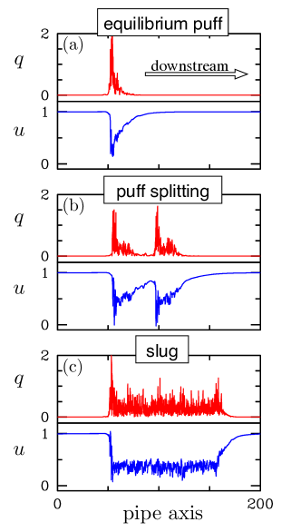
Figure 1: Regimes of transitional pipe flow from simulations in a periodic pipe 200D long. Shown are instantaneous values of turbulence intensity $q$ and axial velocity $u$ along the pipe axis. (a) Equilibrium puff at $\mbox{Re}=2000$. (b) Puff splitting at $\mbox{Re}=2275$. (c) Slug flow at $\mbox{Re}=3200$.

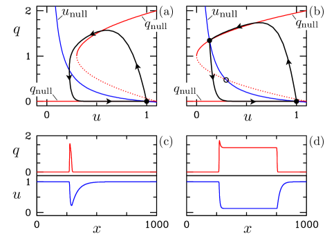
Figure 2: The distinction between puffs and slugs seen as the difference between excitability and bistablilty in the PDE model, Eqs. (1)-(2). Phase planes show nullclines at (a) $r=0.7$ and (b) $r=1$. The fixed point $(1,0)$ corresponds to stable laminar flow. In (a) this is the only fixed point. In (b) the additional stable fixed point corresponds to stable turbulence. Solution snapshots show (c) a puff at $r=0.7$ and (d) a slug at $r=1$. These solutions are plotted in the phase planes with arrows indicating increasing $x$.

2.2 PDE model

The modeling in Barkley (2011) is based on the following physical features of transitional turbulence in pipes. At the upstream (left in Fig. 2) edge of turbulent patches, laminar flow abruptly becomes turbulent. Energy from the laminar shear is rapidly converted into turbulent motion and this results in a rapid change to the mean shear profile (Wygnanski & Champagne, 1973; Hof et al., 2010). In the case of puffs, the turbulent profile is not able to sustain turbulence and thus there is a reverse transition (Wygnanski & Champagne, 1973; Narasimha & Sreenivasan, 1979) from turbulent to laminar flow on the downstream side of a puff. In the case of slugs, the turbulent shear profile can sustain turbulence indefinitely; there is no reverse transition and slugs grow to arbitrary streamwise length (Wygnanski & Champagne, 1973; Nishi et al., 2008). On the downstream side of turbulent patches the mean shear profile recovers slowly (Narasimha & Sreenivasan, 1979), seen in the behavior of $u$ in Fig. 1. The degree of recovery dictates how susceptible the flow is to re-excitation into turbulence (Hof et al., 2010).

The following partial-differential equation (PDE) model captures the essence of these physical features:

$$\partial_{t}q+U\partial_{x}q = q\left(u+r-1-(r+\delta)(q-1)^{2}\right)+\partial_{xx}q,$$ (1)

$$\partial_{t}u+U\partial_{x}u = \epsilon_{1}(1-u)-\epsilon_{2}uq-\partial_{x}u.$$ (2)

In the model, the parameter $r$ plays the role of Reynolds number Re. $U$ accounts for downstream advection by the mean velocity, and is otherwise dynamically irrelevant since it can be removed by a change of reference frame. The model includes minimum derivatives, $q_{xx}$ and $u_{x}$, needed for turbulent regions to excite adjacent laminar ones and for left-right symmetry breaking.

The core of the model is seen in the $q$-$u$ phase plane in Fig. 2. The trajectories are organized by the nullclines: curve where $\dot{u}=0$ and $\dot{q}=0$ for the local dynamics ($q_{xx}=q_{x}=u_{x}=0$). For all $r$ the nullclines intersect in a stable, but excitable, fixed point corresponding to laminar parabolic flow. The $u$ dynamics with $\epsilon_{2}>\epsilon_{1}$ captures in the simplest way the behavior of the mean shear. In the absence of turbulence ($q=0$), $u$ relaxes to $u=1$ at rate $\epsilon_{1}$, while in response to turbulence ($q>0$), $u$ decreases at a faster rate dominated by $\epsilon_{2}$. Values $\epsilon_{1}=0.04$ and $\epsilon_{2}=0.2$ give reasonable agreement with pipe flow. The $q$-nullcline consists of $q=0$ (turbulence is not spontaneously generated from laminar flow) together with a parabolic curve whose nose varies with $r$, while maintaining a fixed intersection with $q=0$ at $u=1+\delta$, ($\delta=0.1$ is used here). The upper branch is attractive, while the lower branch is repelling and sets the nonlinear stability threshold for laminar flow. If laminar flow is perturbed beyond the threshold (which decreases with $r$ like $r^{-1}$), $q$ is nonlinearly amplified and $u$ decreases in response.

The (excitable) puff regime occurs for $r<r_{c}\simeq\epsilon_{2}/(\epsilon_{1}+\epsilon_{2})$, Figs. 2(a) and (c). The upstream side of a puff is a trigger front  (Tyson & Keener, 1988) where abrupt laminar to turbulent transition takes place. However, turbulence cannot be maintained locally following the drop in the mean shear. The system relaminarizes (reverse transition) on the downstream side in a phase front (Tyson & Keener, 1988) whose speed is set by the upstream front. Following relaminarization, $u$ relaxes and laminar flow regains susceptibility to turbulent perturbations. The slug regime occurs for $r>r_{c}$, Figs. 2(b) and (d). The nullclines intersect in additional fixed points. The system is bistable and turbulence can be maintained indefinitely in the presence of modified shear. Both the upstream and downstream sides are trigger fronts, moving at different speeds, giving rise to an expansion of turbulence.

2.3 SPDE model

While the PDE model captures the essence of the puff-slug transition, the model of turbulence is too simple to capture features such as puff decay and puff splitting. In Barkley (2011), a more realistic model was obtained by employing a tent map to mimic shear turbulence. The map was designed to give a local phase-space structure similar to the nullcline picture for the PDE seen in Fig. 2, with the exception that the upper turbulent branch is instead a region of transient chaos. This approach was motivated by the view that shear turbulence is locally a chaotic saddle (Eckhardt et al., 2007) and it naturally extends previous ideas of modeling chaotic transients with maps (Chaté & Manneville, 1988; Bottin & Chaté, 1998; Vollmer et al., 2009). The resulting model has the advantage of being deterministic, as is fluid flow, at least at the level of the Navier-Stokes equations.

Here I consider an alternative approach and model turbulence as noise. This is at the other extreme from the low-dimensional map. Here the dynamics is infinite dimensional and not deterministic. The simplest approach is to apply noise to the $q$ equation and assume it is proportional to $q$ itself. This leads to the following stochastic PDE (SPDE) model:

$$\partial_{t}q+U\partial_{x}q = q\left(u+r-1-(r+\delta)(q-1)^{2}\right)+\partial_{xx}q+\sigma q\eta,$$ (3)

$$\partial_{t}u+U\partial_{x}u = \epsilon_{1}(1-u)-\epsilon_{2}uq-\partial_{x}u.$$ (4)

where $\eta=\eta(x,t)$ is Gaussian noise. The parameter $\sigma$ controls the noise strength. In reality, shear turbulence has significant correlations on the scale of a puff, but these correlations are not considered here and $\eta(x,t)$ taken here to be space-time white.

A large advantage of modeling the effect of turbulence through a noise term is that one has a direct connection to the simple PDE model. Moreover, analysis of the SPDE is likely to be easier than analysis of the deterministic map model. The price is the loss of deterministic dynamics.

Figures 4 and 4 show the regimes of transitional pipe flow from simulations of Eqs. (3)-(4). The deterministic parameters are as before: $\epsilon_{1}=0.04$, $\epsilon_{2}=0.2$, and $\delta=0.1$. The noise strength is $\sigma=1.4$. Figure 4 shows solution snapshots in terms of the model variable $q$ and $u$. Puffs, puff splitting, and slugs are found very similar to those observed in full DNS (see Fig. 2) and in the deterministic map model (see Barkley, 2011). The dynamics of the different regimes is seen in the space-time plots of Fig. 4. At low $r$, puffs are metastable. They persist for long times before abruptly decaying. For intermediate $r$, puff splitting occurs. New puffs are spontaneously nucleated downstream of existing puffs and the system evolves to an intermittent mixture of turbulent and laminar phases. At larger $r$, slugs are observed which differ from the deterministic PDE mainly in that they first occur at larger $r$ and the upper branch is noisy rather than constant. An investigation of the lifetime statistics of puff decay and puff splitting in the SPDE is currently underway.

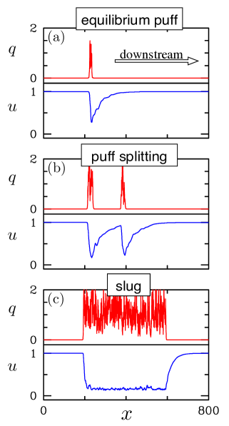
Figure 3: Three regimes of transitional pipe flow from simulations of the SPDE  (3)-(4). Shown are instantaneous values of $q$ and $u$. (a) Puff at $r=0.7$. (b) Puff splitting at $r=0.94$. (c) Slug at $r=1.2$.

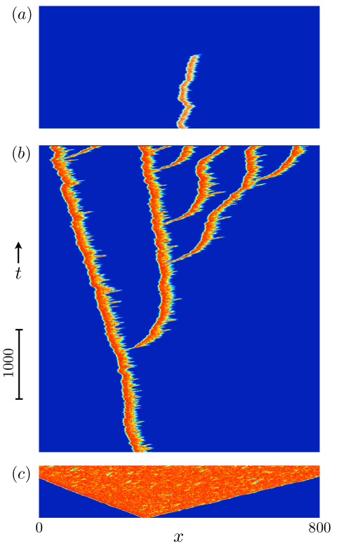
Figure 4: Space-time diagrams illustrate (a) decaying puff at $r=0.7$, (b) puff splitting at $r=0.94$, and (c) slug formation at $r=1.2$. Turbulence intensity $q$ is plotted on a logarithmic scale in a frame co-moving with structures.

While all three regions shown in Figs. 4 and 4 strongly resemble their counterparts in full DNS and experiment, the splitting regime is particularly significant and worthy of further comment. Unlike for puffs and slugs, which are essentially contained in the model by construction, splitting is seen to arise naturally from the elementary puff-slug transition in the presence of complex turbulent dynamics (either noise as here or chaotic dynamics as in Barkley (2011)). The space-time plot in Fig. 4(b) could easily be mistaken for the corresponding plot from full DNS (e.g. see Avila et al., 2011). Sufficient turbulence occasionally escapes from the irregular downstream side of a puff to nucleate a new puff downstream. Visually, this is just as in real pipe flow and is a strong qualitative validation of this modeling approach.

3 Model for plane Couette flow

One of the main difficulties in extending these ideas to other shear flows, such as channel flow or plane Couette flow, is the complexity of the mean flow in these cases (Barkley & Tuckerman, 2007). It is not clear at the present time whether one can adequately model the mean shear in these flows using simple scalar fields. Nevertheless, I discuss here some preliminary ideas on how plane Couette flow might be approached within this modeling framework.

Figure 6 shows a sketch for plane Couette flow. A turbulent patch (red) is shown surrounded to the left and right by laminar flow. One can view this as a cut through a single turbulent band in the striped regime or through a localized patch of turbulence (Prigent et al., 2002; Barkley & Tuckerman, 2005). However, the model is rather crude at present and the important three-dimensional aspects of the problem are not taken into account.

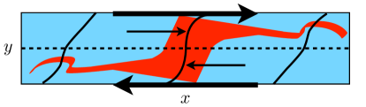
Figure 5: Sketch of plane Couette flow. The shaded region (red) represents a turbulent patch surrounded by laminar flow. Arrows indicate the motion of the bounding plates and the direction of the mean flow in the upper and lower halves of the domain. Three shear profiles are sketched. The $x$-coordinate is centered on the time-averaged flow which has centro-symmetry.

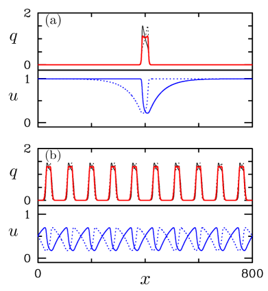
Figure 6: Solutions of the plane Couette model, Eqs. (5)-(8). (a) Localized state at $r=0.7$ and (b) periodic state at $r=0.9$. Solid (dotted) curves represent variables in the upper (lower) half of the domain. The mean turbulence, $(q_{1}+q_{2})/2$, is plotted in bold (red).

Recall that the geometry of plane Couette flow has translation symmetry in the streamwise direction $x$ and also centro-symmetry (rotation by $\pi$) about any point on the midplane $y=0$. Taking the point to be at $x=0$, the centro-symmetry is the transformation $(x,y)\to(-x,-y)$. Time averaged turbulent-laminar patterns break translational symmetry, but do not break centro-symmetry (Barkley & Tuckerman, 2007).

The idea is to model intermittent turbulence in plane Couette flow as two layers, each described by one-dimensional equations similar to those for pipe flow. The turbulence in the two layers is assumed to be coupled. Taking into account that the mean advection in the bottom layer is opposite to that in the top layer, I propose the following PDE model

$$\partial_{t}q_{1}+U\partial_{x}q_{1} = q_{1}\left(u_{1}+r-1-(r+\delta)(q_{1}-1)^{2}\right)+\partial_{xx}q_{1}+\kappa(q_{2}-q_{1}),$$ (5)

$$\partial_{t}u_{1}+U\partial_{x}u_{1} = \epsilon_{1}(1-u_{1})-\epsilon_{2}u_{1}q_{1}-\partial_{x}u_{1},$$ (6)

$$\partial_{t}q_{2}-U\partial_{x}q_{2} = q_{2}\left(u_{2}+r-1-(r+\delta)(q_{2}-1)^{2}\right)+\partial_{xx}q_{2}+\kappa(q_{1}-q_{2}),$$ (7)

$$\partial_{t}u_{2}-U\partial_{x}u_{2} = \epsilon_{2}(1-u_{2})-\epsilon_{2}u_{2}q_{2}+\partial_{x}u_{2}.$$ (8)

where $q_{1}$ and $u_{1}$ are the turbulence and mean shear in the upper layer and $q_{2}$ and $u_{2}$ are the turbulence and mean shear in the lower layer. These equations are symmetric under translation in $x$ and the reflection defined by $(x,q_{1},u_{1},q_{2},u_{2})\to(-x,q_{2},u_{2},q_{1},u_{1})$, which is the model equivalent of centro-symmetry.

Figure 6 shows solutions to Eqs. (5)-(8) with $U=1$ and the coupling constant $\kappa=0.1$. Other parameter values are the same as for the model pipe simulations. For small $r$, stable localized states appear from localized perturbations of laminar flow. At $r\simeq 0.75$ the localized states became unstable and spread to form a periodic alternation of turbulent and laminar phases. The localized and periodic structures both have centro-symmetry.

The choice of $U$ and the coupling parameter $\kappa$ are probably rather important in obtaining steady patterns. The effect of noise is also not yet fully understood as this investigation is still in a preliminary stage.

4 Conclusion

I have presented models of parallel shear flows in two scalar variables – turbulence and mean shear. The model for pipe flow is based closely on physical features of transitional turbulence and it reproduces nearly all large-scale features of transitional pipe flow. The model for plane Couette flow necessarily misses many features of the real flow since the model is only one dimensional, whereas plane Couette flow has two extended dimensions. Nevertheless, the plane Couette flow model is an important starting point for further investigations of this and other parallel shear flows such as plane channel and boundary layer flow.

References

- Avila et al. (2011) Avila, K., Moxey, D., de Lozar, A., Avila, M., Barkley, D. & Hof, B. 2011 Onset of sustained turbulence in pipe flow. Science 333, 192–196.
- Avila et al. (2010) Avila, M., Willis, A. P. & Hof, B. 2010 On the transient nature of localized pipe flow turbulence. J. Fluid Mech. 646, 127–136.
- Barkley (2011) Barkley, D. 2011 Simplifying the complexity of pipe flow. Phys. Rev. E 84, 016309.
- Barkley & Tuckerman (2005) Barkley, D. & Tuckerman, L. 2005 Computational study of turbulent laminar patterns in Couette flow. Phys. Rev. Lett. 94, 014502.
- Barkley & Tuckerman (2007) Barkley, D. & Tuckerman, L. S. 2007 Mean flow of turbulent–laminar patterns in plane Couette flow. J. Fluid Mech. 576, 109–137.
- Blackburn & Sherwin (2004) Blackburn, H.M. & Sherwin, S.J. 2004 Formulation of a Galerkin spectral element-Fourier method for three-dimensional incompressible flows in cylindrical geometries. J. Comput. Phys. 197, 759–778.
- Bottin & Chaté (1998) Bottin, S. & Chaté, H. 1998 Statistical analysis of the transition to turbulence in plane Couette flow. Eur. Phys. J. B 6, 143–155.
- Chaté & Manneville (1988) Chaté, H. & Manneville, P. 1988 Spatio-temporal intermittency in coupled map lattices. Physica D 32, 409–422.
- Darbyshire & Mullin (1995) Darbyshire, A.G. & Mullin, T. 1995 Transition to turbulence in constant-mass-flux pipe-flow. J. Fluid Mech. 289, 83–114.
- Eckhardt et al. (2007) Eckhardt, B., Schneider, T. M., Hof, B. & Westerweel, J. 2007 Turbulence transition in pipe flow. Annu. Rev. Fluid Mech. 39, 447–468.
- Faisst & Eckhardt (2004) Faisst, H. & Eckhardt, B. 2004 Sensitive dependence on initial conditions in transition to turbulence in pipe flow. J. Fluid Mech. 504, 343–352.
- Hof et al. (2010) Hof, B., de Lozar, A., Avila, M., Tu, X. & Schneider, T. M. 2010 Eliminating turbulence in spatially intermittent flows. Science 327, 1491–1494.
- Hof et al. (2008) Hof, B., de Lozar, A., Kuik, D. & Westerweel, J. 2008 Repeller or attractor? selecting the dynamical model for the onset of turbulence in pipe flow. Phys. Rev. Lett. 101, 214501.
- Hof et al. (2006) Hof, B., Westerweel, J., Schneider, T. M. & Eckhardt, B. 2006 Finite lifetime of turbulence in shear flows. Nature (London) 443, 59–62.
- Kuik et al. (2010) Kuik, D. J., Poelma, C. & Westerweel, J. 2010 Quantitative measurement of the lifetime of localized turbulence in pipe flow. J. Fluid Mech. 645, 529–539.
- Moxey & Barkley (2010) Moxey, D. & Barkley, D. 2010 Distinct large-scale turbulent-laminar states in transitional pipe flow. Proc. Natl. Acad. Sci. USA 107, 8091–8096.
- Mullin (2011) Mullin, T. 2011 Experimental studies of transition to turbulence in a pipe. Annu. Rev. Fluid Mech. 43, 1–24.
- Narasimha & Sreenivasan (1979) Narasimha, R. & Sreenivasan, K.R. 1979 Relaminarization of fluid flows. Adv. in Appl. Mech. 19, 221–309.
- Nishi et al. (2008) Nishi, M., Ünsal, B., Durst, F. & Biswas, G. 2008 Laminar-to-turbulent transition of pipe flows through puffs and slugs. J. Fluid Mech. 614, 425.
- Peixinho & Mullin (2006) Peixinho, J. & Mullin, T. 2006 Decay of turbulence in pipe flow. Phys. Rev. Lett. 96, 094501.
- Prigent et al. (2002) Prigent, A., Gregoire, G., Chaté, H., Dauchot, O. & van Saarloos, W. 2002 Large-scale finite-wavelength modulation within turbulent shear flows. Phys. Rev. Lett. 89, 014501.
- Reynolds (1883) Reynolds, O. 1883 An experimental investigation of the circumstances which determine whether the motion of water shall be direct or sinuous, and of the law of resistance in parallel channels. Philos. Trans. R. Soc. London A 174, 935–982.
- Rotta (1956) Rotta, J 1956 Experimenteller beitrag zur entstehung turbulenter strömung im rohr. Ing-Arch. 24, 258–281.
- Schneider & Eckhardt (2008) Schneider, T. M. & Eckhardt, B. 2008 Lifetime statistics in transitional pipe flow. Phys. Rev. E 78, 046310.
- Tillmark & Alfredsson (1992) Tillmark, N. & Alfredsson, P. H. 1992 Experiments on transition in plane Couette flow. J. Fluid Mech. 235, 89–102.
- Tyson & Keener (1988) Tyson, J.J. & Keener, J.P. 1988 Singular perturbation-theory of traveling waves in excitable media. Physica D 32, 327–361.
- Vollmer et al. (2009) Vollmer, J., Schneider, T. M. & Eckhardt, B. 2009 Basin boundary, edge of chaos and edge state in a two-dimensional model. New J. Phys. 11, 013040.
- Willis & Kerswell (2007) Willis, A. P. & Kerswell, R. R. 2007 Critical behavior in the relaminarization of localized turbulence in pipe flow. Phys. Rev. Lett. 98, 014501.
- Wygnanski & Champagne (1973) Wygnanski, I. & Champagne, H. 1973 Transition in a pipe. part 1. origin of puffs and slugs and flow in a turbulent slug. J. Fluid Mech. 59, 281–335.
- Wygnanski et al. (1975) Wygnanski, I., Sokolov, M. & Friedman, D. 1975 Transition in a pipe .2. equilibrium puff. J. Fluid Mech. 69, 283–304.
- Wygnanski et al. (1976) Wygnanski, I., Sokolov, M. & Friedman, D. 1976 On a turbulent ’spot’ in a laminar boundary layer. J. Fluid Mech. 78, 785–819.