Self-similar Solutions to a Kinetic Model for Grain Growth

Abstract

We prove the existence of self-similar solutions to the Fradkov model for two-dimensional grain growth, which consists of an infinite number of nonlocally coupled transport equations for the number densities of grains with given area and number of neighbours (topological class). For the proof we introduce a finite maximal topological class and study an appropriate upwind-discretization of the time dependent problem in self-similar variables. We first show that the resulting finite dimensional differential system has nontrivial steady states. Afterwards we let the discretization parameter tend to zero and prove that the steady states converge to a compactly supported self-similar solution for a Fradkov model with finitely many equations. In a third step we let the maximal topology class tend to infinity and obtain self-similar solutions to the original system that decay exponentially. Finally, we use the upwind discretization to compute self-similar solutions numerically.

Keywords:

grain growth, kinetic model, self-similar solution

MSC (2010):

34A12, 35F25, 35Q82, 74A50

1 Introduction

Grain growth denotes the late stage coarsening of polycrystalline materials when migration of grain boundaries due to capillary forces causes small grains to vanish and larger grains to grow. One often observes that despite having different histories many materials eventually exhibit universal statistically self-similar coarsening behaviour, usually referred to as normal grain growth. Different approaches have been used to predict and explain this phenomenon, see [2, 3] for Monte-Carlo methods, [14] for a study of vertex models, and more recently [7, 8] for boundary tracking methods. We also refer to the theoretical approach in [4, 5], which is based on the grain boundary character distribution.

However, it remains a challenge to establish such universal long-time asymptotics in mathematical models and it is often difficult to prove only the existence of self-similar solutions. In this article we investigate the existence of self-similar solutions to a kinetic mean-field model that has been suggested by Fradkov [10] to describe grain growth in two dimensions.

1.1 Fradkov’s mean-field model

We briefly describe the derivation of Fradkov’s model and refer to [10, 11, 12] for more details. Our starting point are two-dimensional periodic networks of grain boundaries that meet in triple junctions (Fig. 1). In the case of constant surface energy and infinite mobility of triple junctions, the grain boundaries move according to the mean curvature flow while all angles at the triple junctions are $2\pi/3$.

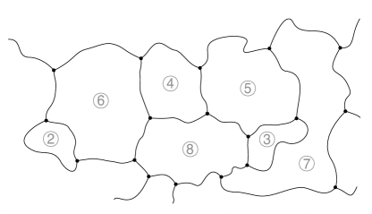
Figure 1: Cartoon of a 2D network of grains with triple junctions, where the Herring condition implies that all angles are equal to $2\pi/3$. The encircled numbers refer to the topology classes.

In this setting one can easily derive the von Neumann–Mullins law for the area $a(t)$ at time $t>0$ of a single grain with $n$ edges [17]:

$$\frac{\,\mathrm{d}}{\,\mathrm{d}t}a\left(t\right)=M\sigma\frac{\pi}{3}\left(n-6\right)\,.$$ (1)

Here $M$ denotes the mobility of the grain boundaries and $\sigma$ the surface tension.

Figure 2: Neighbour switching

The evolution of such a network by mean curvature is well–defined [15, 16] until two vertices on a grain boundary collide, after which topological rearrangements may take place. If an edge vanishes an unstable fourfold vertex is produced, which immediately splits up again such that two new vertices are connected by a new edge. As a consequence two neighbouring grains decrease their topological class (i.e., the number of edges), whereas the other two grains increase it (Fig. 2). Furthermore, grains can vanish such that some vertices and edges disappear. Due to the von Neumann–Mullins law this can only happen for grains with topological class $2\leq n\leq 5$. As illustrated in Fig. 3, the vanishing of a grain of topological class $n=4$ or $n=5$ can result in topologically different configurations.

Figure 3: Grain vanishing

In order to derive a kinetic description of the evolution of the grain boundary network we introduce the number densities ${f_{n}\left(a,t\right)}$ of grains with topological class $n\geq 2$ and area $a\geq 0$ at time $t\geq 0$. As long as no topological rearrangements take place, the von Neumann–Mullins law (1) implies that $f_{n}$ evolves according to

$$\partial_{t}{f_{n}\left(a,t\right)}+\left(n-6\right)\partial_{a}{f_{n}\left(a,t\right)}=0\,.$$

This equation needs to be supplemented with boundary conditions at $a=0$ for $n>6$. It is reasonable to assume that no new grains are created during the coarsening process, which implies that

$${f_{n}\left(0,t\right)}=0\quad\quad\text{for}\quad n\geq 7\,.$$ (2)

To model the topological changes we define a collision operator $\tilde{J}$ that couples the equations for different topological classes. More precisely, we introduce topological fluxes $\eta_{n}^{+}$ and $\eta_{n}^{-}$ that describe the flux from class $n$ to $n+1$ and from $n$ to $n-1$, respectively, and set

$$(\tilde{J}f)_{n}=\eta_{n-1}^{+}+\eta_{n+1}^{-}-\eta_{n}^{+}-\eta_{n}^{-}\,$$

with $\eta_{1}^{+}=\eta_{2}^{-}=0$ due to $n\geq 2$. Employing a mean-field assumption Fradkov [10] suggests that the fluxes are given by

$$\eta_{n}^{+}=\Gamma\beta\,nf_{n}\,,\qquad\eta_{n}^{-}=\Gamma\left(\beta+1\right)nf_{n},$$ (3)

where the coupling weight $\Gamma$ describes the intensity of topological changes and depends on the complete state of the system in a self–consistent way, see (6) below. Moreover, the parameter $\beta$ measures the ratio between switching events and vanishing events. Our analysis requires $\beta\in(0,2)$, but the numerical simulations work well also for larger $\beta$.

Although Fradkov’s model has no upper bound for the topology class $n$, it is convenient for the mathematical analysis to consider variants of the model with $2\leq{n}\leq{N}$ for some $6<N<\infty$. In this case we close the equations for $(f_{n})_{2\leq n\leq N}$ by assuming $\eta_{N+1}^{-}=\eta_{N}^{+}=0$.

Assumption (3) implies that the collision terms are given by $\tilde{J}f=\Gamma{Jf}$ with

$$\begin{split}{\left({Jf}\right)}_{2}&=3\left(\beta+1\right)f_{3}-2\beta f_{2},\\ {\left({Jf}\right)}_{n}&=\left(\beta+1\right)\left(n+1\right)f_{n+1}-\left(2\beta+1\right)n\,f_{n}+\beta\left(n-1\right)f_{n-1}\quad\text{for}\quad{}2<n<N-1,\\ {\left({Jf}\right)}_{N}&=\beta(N{-}1)f_{N{-}1}-(\beta+1)Nf_{N},\end{split}$$ (4)

where the last identify is not used for $N=\infty$. Notice that this definition ensures the zero balance property

$$\sum\limits_{n=2}^{N}\left(Jf\right)_{n}{\left({a},\,{t}\right)}=0\qquad\text{for all}\quad a,\,t>0,$$

which reflects that the number of grains with given area does not change due to switching or vanishing events. To summarize, the kinetic model we consider in this paper is given by

$$\partial_{t}{f_{n}\left(a,t\right)}+\left(n-6\right)\partial_{a}{f_{n}\left(a,t\right)} =\Gamma{\big{(}f{\left({t}\right)}\big{)}}{\left(Jf\right)_{n}\left(a,t\right)}\,,\qquad(a,t)\in(0,\infty)^{2}\,,\;n\geq 2,$$ (5)

with boundary conditions (2), either $N<\infty$ or $N=\infty$, and $(Jf)_{n}$ given by (4).

It remains to determine the coupling weight $\Gamma$ in dependence of $f$. The key idea is to choose $\Gamma$ such that the total area

$$A(t)=\sum_{n=2}^{N}Y_{n}(t)\qquad\mbox{ with }\qquad Y_{n}(t)=\int_{0}^{\infty}af_{n}(a,t)\,\,\mathrm{d}a$$

is conserved during the evolution. One easily checks that $dA/dt=P$, where $P$ is the polyhedral defect defined by

$$P(t)=\sum_{n=2}^{N}{\left({n-6}\right)}X_{n}(t)\qquad\mbox{ with }\qquad X_{n}(t)=\int_{0}^{\infty}f_{n}(a,t)\,\,\mathrm{d}a.$$

The polyhedral formula $P=0$ resembles Euler’s formula for networks with triple junctions and states that the average number of neighbours per grain is $6$. We now readily verify that $dP/dt=0$ holds if and only if

$$\Gamma\big{(}f(t)\big{)}=\frac{\sum\limits_{n=2}^{5}\left(n-6\right)^{2}f_{n}(0,t)}{\beta{N}X_{N}(t)-2\left(\beta+1\right)X_{2}(t)+\sum\limits_{n=2}^{N}nX_{n}(t)}\,,$$ (6)

where we use the convention $NX_{N}=0$ for $N=\infty$. In particular, (6) guarantees the conservation of area and the polyhedral formula provided that the initial data satisfy $P=0$.

We finally mention that well-posedness of Fradkov’s model, both for $N<\infty$ and $N=\infty$, has been established in [12] for $\beta\in(0,2)$. A similar model with finite $N$ has been considered in [6].

1.2 Self-similar solutions and main result

Self-similar solutions to (5) take the form

$$f_{n}(a,t)=\frac{g_{n}{\left({\xi}\right)}}{t^{2}}\,,\qquad\xi=\frac{a}{t}\geq 0\,,$$

where the sequence $g=(g_{n})_{n\geq 2}$ of self-similar profiles satisfies

$$-2g_{n}-\big{(}\xi+6-n\big{)}g_{n}^{\prime}=\Gamma\big{(}Jg\big{)}_{n}\,$$ (7)

for some positive constant $\Gamma$ as well as the boundary conditions $g_{n}{\left({0}\right)}=0$ for $n>6$. With some abuse of notation, we define the moments

$$X_{n}=\int_{0}^{\infty}g_{n}(\xi)\,d\xi\qquad\mbox{ and }\qquad Y_{n}=\int_{0}^{\infty}\xi g_{n}(\xi)\,d\xi,$$

and refer to

$$P=\sum_{n=2}^{N}{\left({n-6}\right)}X_{n}\qquad\mbox{ and }\qquad A=\sum_{n=2}^{N}Y_{n}$$

as the polyhedral defect and the area of a self-similar solution, respectively.

It is important to note that each sufficiently integrable solution to (1.2) satisfies the analogue of the polyhedral formula, and that the coupling weight $\Gamma$ depends on the $g_{n}$’s in a self-consistent manner. In fact, multiplying (7) by $\xi$, integrating with respect to $\xi$, and summing over $n$, we find that the zero balance property of $J$ implies $P=0$. Similarly, if we multiply by $1$ instead of $\xi$, we easily derive the analogue to (6), that means we have $\Gamma{\left({g}\right)}=\Gamma_{\rm num}{\left({g}\right)}/\Gamma_{\rm den}{\left({g}\right)}$ with

$$\Gamma_{\rm num}{\left({g}\right)}=\sum\limits_{n=2}^{5}\left(n-6\right)^{2}g_{n}(0)\,,\qquad\Gamma{\left({g}\right)}=\beta{N}X_{N}-2\left(\beta+1\right)X_{2}+\sum\limits_{n=2}^{N}nX_{n}\,.$$ (8)

The main mathematical difficulty in the existence proof for self-similar solutions stems from the fact that the ordinary differential equation (7) is singular at $\xi=n-6$ and has different transport directions for $\xi<n-6$ and $\xi>n-6$. In this paper we prove the existence of weak self-similar solutions for both $N<\infty$ and $N=\infty$, where weak solution means that each function $g_{n}$ satisfies

$$\int_{0}^{\infty}g_{n}{\big{(}{\left({\xi+6-n}\right)}\phi^{\prime}-\phi\big{)}}\,\mathrm{d}\xi+(6-n)_{+}\,g_{n}(0)\phi(0)=\Gamma(g)\int_{0}^{\infty}\big{(}Jg\big{)}_{n}\phi\,\mathrm{d}\xi$$ (9)

for all smooth test functions $\phi$ with compact support in $[0,\,\infty)$.

Our existence result can be summarized as follows.

Theorem 1.

Let $\beta\in(0,2)$ and assume that either $6<N<\infty$ or $N=\infty$. Then, there exists a weak self-similar solution to the Fradkov model that is nontrivial and nonnegative with finite area, and satisfies

$$\sum_{n=2}^{N}\Big{(}e^{\lambda n}X_{n}+\int_{0}^{\infty}e^{\lambda\xi}g_{n}(\xi)\,d\xi\Big{)}<\infty$$

for all $0<{\lambda}<\ln{\left({1+1/\beta}\right)}$. Moreover, for $N<\infty$ all functions $g_{n}$ are supported in $[0,\,N-6]$.

These main assertions can be supplemented by the following remarks.

1. Since $\Gamma(g)$ depends on $g$ homogeneously of order $0$, the set of self-similar solutions is invariant under scalings $g_{n}\rightsquigarrow{\lambda}{g_{n}}$ with ${\lambda}>0$. Therefore we can normalize self-similar solutions by prescribing the area.

2. The weak formulation combined with the integrability condition $g_{n}\in{\mathsf{L}}^{1}(0,\infty)$ implies regularity results. Specifically, in a first step we find that each function $g_{n}$ is continuous at all points $\xi\in[0,\,\infty)\setminus\{n-6\}$. Using this we then easily show in a second step that $g_{n}$ is even continuously differentiable at all points $\xi\in[0,\,\infty)\setminus\{n-7,n-6,n-5\}$. We also establish further regularity results that characterize the behaviour of $g_{n}$ near $\xi=n-6$, see Lemma 19, and find for large $n$ that $g_{n}$ is continuous also at $\xi=n-6$.

3. The moment estimates from Theorem 1 imply that $g_{n}$ decays exponentially in $\xi$. More precisely, multiplying (7) with $e^{{\lambda}\xi}$ and integrating over $[\xi,\,\infty)$ gives $g_{n}{\left({\xi}\right)}\leq{C}_{n}e^{{\lambda}\xi}$ for some constant $C_{n}$ and all $\xi$.

4. Numerical simulations as described in Section 4 indicate, at least for $N<\infty$, that for each $\beta$ there exists a unique self-similar solution with prescribed area, but we are not able to prove this.

Our strategy for proving Theorem 1 is inspired by the existence proof for self-similar solutions to coagulation equations in [9]. In Section 2 we introduce a finite-dimensional dynamical model that can be regarded as a semi-discrete upwind scheme for (5) in self-similar variables, and involves the discretization length $0<{\varepsilon}\ll 1$. To derive this scheme we assume that $N<\infty$, restrict the rescaled area variable $\xi$ to a finite domain $[0,\,L]$ with sufficiently large $L$, and impose artificial Dirichlet conditions at $\xi=L$. Moreover, we identify a discrete analogue to (6) that ensures the conservation of both area and polyhedral formula. Standard results from the theory of dynamical systems then imply the existence of nontrivial steady states for each sufficiently small ${\varepsilon}$.

Afterwards we show that these steady states converge as ${\varepsilon}\to 0$ to a self-similar profile for the Fradkov model for $N<\infty$. The proof of this assertion combines two different arguments: First, in Section 3.1 we derive suitable a priori estimates that allow us to extract convergent subsequences whose limits provide candidates for the self-similar profiles. Second, in Section 3.2 we analyse the behaviour near the singular points $\xi=n-6$ in order to rule out that Dirac masses appear in the limit.

In Section 3.3 we establish the exponential decay of $X_{n}$ and derive uniform estimates for higher moments. The resulting tightness estimates then enable us to pass to the limit $N\to\infty$ in Section 3.4. Finally, in Section 4 we illustrate that the upwind discretization of (5) in self-similar variables, combined with explicit Euler steps for the time discretization, provides a convenient algorithm for the numerical computations of self-similar solutions.

2 The discrete dynamical model

In order to prove the existence of self-similar solutions we study an upwind finite-difference discretization of the time-dependent problem in self-similar variables. To that aim we restrict the rescaled area variable $\xi$ to a finite interval $[0,L]$ with $L\in{\mathbb{N}}$ and $L>{N-6}$, and for each $K\in{\mathbb{N}}L$ we consider the grid points $\xi_{k}=kL/K$, such that

$$\xi_{k+1}-\xi_{k}=L/K=:{\varepsilon}.$$

Notice that for each $n>6$ the critical area $\xi={n-6}$ corresponds to one of the grid points, that means for each $n\geq 2$ we have

$$\xi_{k_{n}}=n-6,\qquad k_{n}:={\left({n-6}\right)}K/L$$

with $k_{6}=0$, $k_{n}<0$ for $n=2{...}{5}$, and $0<k_{n}<K$ for $n=7{...}{N}$.

Using the difference operators $\nabla^{-}$ and $\nabla^{+}$ with

$$\nabla^{+}u^{k}=\frac{u^{k+1}-u^{k}}{{\varepsilon}},\qquad\nabla^{-}u^{k}=\frac{u^{k}-u^{k-1}}{{\varepsilon}},\qquad$$

we mimic the transport term $-{\left({\xi+6-n}\right)}g_{n}^{\prime}{\left({\xi}\right)}$ by the upwind discretization

$$-{\left({\xi_{k}+6-n}\right)}_{+}\nabla^{+}g_{n}^{k}+{\left({\xi_{k}+6-n}\right)}_{-}\nabla^{-}g_{n}^{k}+\delta_{k}^{k_{n}}{g_{n}^{k}}.$$ (10)

Here $\delta_{k}^{k_{n}}$ is the usual Kronecker delta and ${x}_{\pm}$ denotes the positive and negative part of $x$, that means ${x}_{\pm}=\max\{\pm{x},\,0\}\geq 0$ and $x={x}_{+}-{x}_{-}$.

At a first glance, the Kronecker delta in (10) seems to be quite artificial, but it is naturally related to the singularity of the transport operator. More precisely, for a continuous variable $\xi$ one easily shows that

$$-{\left({\xi+6-n}\right)}\delta^{\prime}_{n-6}{\left({\xi}\right)}=\delta_{n-6}{\left({\xi}\right)}$$

holds in the sense of distributions, where $\delta_{n-6}{\left({\xi}\right)}$ is the Dirac distribution supported in $\xi=n-6$. Our discretization of the transport operator satisfies a similar identity which can be seen by setting $g_{n}^{k}={\varepsilon}^{-1}\delta_{n}^{k_{n}}$ in (10). The Kronecker delta in (10) therefore guarantees that the resulting discrete scheme resembles the continuous dynamics even if mass is concentrated near the singularities.

With (10) the discrete dynamical model reads

$$\frac{\,\mathrm{d}missing}{\,\mathrm{d}t}g_{n}^{k}-2g_{n}^{k}-{\left({\xi_{k}+6-n}\right)}_{+}\nabla^{+}g_{n}^{k}+{\left({\xi_{k}+6-n}\right)}_{-}\nabla^{-}g_{n}^{k}+\delta_{k}^{k_{n}}{g_{n}^{k}}=\Gamma(Jg^{k})_{n}\,,$$ (11)

where the coupling weight $\Gamma$ will be defined in Section 2.1. To close the system (11) we impose the boundary conditions

$$g_{n}^{0}=0\qquad\mbox{ for }\;7\leq{n}\leq{N},\qquad\qquad g_{n}^{K}=0\qquad\mbox{ for }\;2\leq{n}\leq{N},$$ (12)

so (11) becomes an evolution equation for the variables $g_{n}^{k}$ with $n=2{...}{N}$ and $k=1{...}{K-1}$. Notice that the boundary conditions for $k=0$ stem naturally from (2), whereas those for $k=K$ reflect the cut off in $\xi$.

2.1 Moment balances and choice of the coupling weight

In complete analogy to the discussion in Section 1 we choose the discrete coupling coefficient $\Gamma$ such that (11) with (12) conserves the area. In order to identify the correct formula we start with an auxiliary result for a discrete moment $Z_{n}$ with

$$Z_{n}:={\varepsilon}\sum_{k=1}^{K-1}\mu_{n}^{k}g_{n}^{k},$$

where $\mu_{n}^{k}$ are arbitrary moment coefficients.

Lemma 2.

We have

$$\frac{\,\mathrm{d}missing}{\,\mathrm{d}t}Z_{n}-2Z_{n}+\zeta_{n}=\Gamma\,{\varepsilon}\sum_{k=1}^{K-1}\mu_{n}^{k}{\big{(}Jg^{k}\big{)}}_{n},$$ (13)

where

$$\zeta_{n}:=(6-n)_{+}\,\mu_{n}^{0}g_{n}^{1}+{\varepsilon}\sum_{k=1}^{K-1}\eta_{n}^{k}g_{n}^{k},\qquad\eta_{n}^{k} :=\left\{\begin{array}[]{lccl}\nabla^{+}[\mu_{n}^{k}{\left({\xi_{k}+6-n}\right)}]&&\text{for}&k<k_{n},\\ \mu_{n}^{k_{n}}&&\text{for}&k=k_{n},\\ \nabla^{-}[\mu_{n}^{k}{\left({\xi_{k}+6-n}\right)}]&&\text{for}&k>k_{n}.\end{array}\right.$$ (17)

Proof.

Multiplying (11) by ${\varepsilon}{\mu_{n}^{k}}$, and summing over $k=1{...}{K-1}$, give (13) with $\zeta_{n}=\zeta^{+}_{n}+\zeta^{-}_{n}+{\varepsilon}{\mu_{n}^{k_{n}}}{g_{n}^{k_{n}}}$ and

$$\zeta^{+}_{n}:=-{\varepsilon}\sum_{k=1}^{K-1}\mu_{n}^{k}{\left({\xi_{k}+6-n}\right)}_{+}\nabla^{+}g_{n}^{k},\qquad\zeta^{-}_{n}:={\varepsilon}\sum_{k=1}^{K-1}\mu_{n}^{k}{\left({\xi_{k}+6-n}\right)}_{-}\nabla^{-}g_{n}^{k}.$$

We now reformulate $\zeta_{n}^{-}$ and $\zeta_{n}^{+}$ by means of the discrete integration by parts formula

$${\varepsilon}\sum_{k=K_{1}}^{K_{2}}v^{k}\nabla^{+}u^{k}+{\varepsilon}\sum_{k=K_{1}}^{K_{2}}u^{k}\nabla^{-}v^{k}=u^{K_{2}+1}v^{K_{2}}-u^{K_{1}}v^{K_{1}-1}\,,\qquad K_{2}\geq K_{1}\geq 1\,.$$

To this end we consider the following two cases:

Case I: $2\leq{n}\leq{6}$. By definition, we have $\xi_{k}+6-n\geq 0$ for all $k=1{...}{K-1}$. This implies $\zeta^{-}_{n}=0$ and hence

$$\zeta^{+}_{n} =-{\varepsilon}\sum_{k=1}^{K-1}\mu_{n}^{k}{\left({\xi_{k}+6-n}\right)}\nabla^{+}g_{n}^{k}={\left({6-n}\right)}\mu_{n}^{0}g_{n}^{1}+{\varepsilon}\sum_{k=1}^{K-1}g_{n}^{k}\nabla^{-}[\mu_{n}^{k}{\left({\xi_{k}+6-n}\right)}],$$

where we used $\xi_{0}=0$ and the boundary condition $g_{n}^{K}=0$.

Case II: $7\leq{n}\leq{N}$. Here we have $1\leq k_{n}<K-1$ with $\xi_{k_{n}}+6-n=0$, and hence

$$\zeta^{+}_{n} =-{\varepsilon}\sum_{k=k_{n}+1}^{K-1}\mu_{n}^{k}{\left({\xi_{k}+6-n}\right)}\nabla^{+}g_{n}^{k}={\varepsilon}\sum_{k=k_{n}+1}^{K-1}g_{n}^{k}\nabla^{-}[\mu_{n}^{k}{\left({\xi_{k}+6-n}\right)}].$$

Similarly, we find

$$\zeta_{n}^{-} =-{\varepsilon}\sum_{k=1}^{k_{n}-1}\mu_{n}^{k}{\left({\xi_{k}+6-n}\right)}\nabla^{-}g_{n}^{k}={\varepsilon}\sum_{k=1}^{k_{n}-1}g_{n}^{k}\nabla^{+}[\mu_{n}^{k}{\left({\xi_{k}+6-n}\right)}]$$

thanks to the boundary conditions $g_{n}^{0}=g_{n}^{K}=0$. ∎

We next summarize some elementary properties of the coupling operator $J$.

Lemma 3.

The coupling matrix $J$ satisfies

$$\sum_{n=2}^{N}\theta_{n}{\left({Jf}\right)}_{n}=\sum_{n=2}^{N-1}{\left({\theta_{n+1}-\theta_{n}}\right)}\beta nf_{n}-\sum_{n=3}^{N}{\left({\theta_{n}-\theta_{n-1}}\right)}(\beta+1)nf_{n},$$

where $\theta_{n}$ denote arbitrary weights. In particular, we have

$$\sum_{n=2}^{N}{\left({Jf}\right)}_{n}=0,\qquad\sum_{n=2}^{N}{\left({6-n}\right)}{\left({Jf}\right)}_{n}=\beta Nf_{N}-\beta 2f_{2}+\sum_{n=3}^{N}nf_{n}.$$ (18)

Proof.

The definitions from (4) imply

$$\sum_{n=2}^{N}\theta_{n}{\left({Jf}\right)}_{n}= \sum_{n=2}^{N-1}\theta_{n}(\beta+1)(n+1)f_{n+1}+\sum_{n=3}^{N}\theta_{n}\beta(n-1)f_{n-1}$$

$$-\sum_{n=2}^{N-1}\theta_{n}\beta nf_{n}-\sum_{n=3}^{N}\theta_{n}(\beta+1)nf_{n},$$

and all claims follow immediately by direct computations. ∎

For the following considerations we introduce the discrete moments

$$X_{n}:={\varepsilon}\sum_{k=1}^{K-1}g_{n}^{k},\qquad Y_{n}:={\varepsilon}\sum_{k=1}^{K-1}\xi_{k}g_{n}^{k}\,$$

as well as the auxiliary quantity

$$Q:={\varepsilon}\sum_{n=2}^{N}\sum_{k=1}^{K-1}\mathrm{sgn}{\left({\xi_{k}+6-n}\right)}g_{n}^{k}.$$

We also define the discrete area and the discrete polyhedral defect by

$$A:=\sum_{n=2}^{N}Y_{n},\qquad P:=\sum_{n=2}^{N}{\left({n-6}\right)}X_{n}.$$

Corollary 4.

We have

$$\frac{\,\mathrm{d}missing}{\,\mathrm{d}t}X_{n} =X_{n}+\Gamma{\left({JX}\right)}_{n}-(6-n)_{+}\,g_{n}^{1}\,,$$ (19)

$$\frac{\,\mathrm{d}missing}{\,\mathrm{d}t}Y_{n} ={\left({n-6}\right)}X_{n}+\Gamma{\left({JY}\right)}_{n}+{\varepsilon}^{2}\sum_{k=1}^{K-1}\mathrm{sgn}{\left({\xi_{k}+6-n}\right)}g_{n}^{k}\,.$$ (20)

Proof.

The claim for $X_{n}$ follows from Lemma 2 since $\mu_{n}^{k}=1$ implies

$$\eta_{n}^{k} =\left\{\begin{array}[]{lclccl}\nabla^{+}[{\xi_{k}+6-n}]&=&1&&\text{for}&k<k_{n},\\ 1&&&&\text{for}&k=k_{n},\\ \nabla^{-}[{\xi_{k}+6-n}]&=&1&&\text{for}&k>k_{n}.\end{array}\right.$$

Similarly, with $\mu_{n}^{k}=\xi_{k}$ we find

$$\eta_{n}^{k} =\left\{\begin{array}[]{lclccl}\nabla^{+}[\xi_{k}{\left({\xi_{k}+6-n}\right)}]&=&2\xi_{k}+{6-n}+{\varepsilon}&&\text{for}&k<k_{n},\\ \xi_{k}&=&2\xi_{k}+{6-n}&&\text{for}&k=k_{n},\\ \nabla^{-}[\xi_{k}{\left({\xi_{k}+6-n}\right)}]&=&2\xi_{k}+{6-n}-{\varepsilon}&&\text{for}&k>k_{n}.\end{array}\right.$$

This means $\eta_{n}^{k}=2\xi_{k}+{6-n}-{\varepsilon}\mathrm{sgn}{\left({\xi_{k}+6-n}\right)}$ for all $n=2{...}{N}$ and $k=1{...}{K-1}$, so Lemma 2 implies (20). ∎

We now show that the initial value problem for the differential system (11) has a global unique solution with state space

$$\mathcal{U}=\left\{{\left({g_{n}^{k}}\right)}_{n=2{...}{N},\,k=1{...}{K-1}}\;:\;A=1,\;P+{\varepsilon}{Q}=0\right\},$$

provided that $\Gamma=\Gamma_{\rm num}/\Gamma_{\rm den}$ is given by

$$\begin{split}\Gamma_{\rm num}&:=\sum_{n=2}^{5}{\left({6-n}\right)}{\left({6-n+{\varepsilon}}\right)}g_{n}^{1},\\ \Gamma_{\rm den}&:=\sum_{n=2}^{N}{\left({6-n}\right)}{\left({JX}\right)}_{n}-{\varepsilon}^{2}\sum_{n=2}^{N}\sum_{k=1}^{K-1}\mathrm{sgn}{\left({\xi_{k}+6-n}\right)}{\big{(}Jg^{k}\big{)}}_{n}.\end{split}$$ (21)

Lemma 5.

Definition (21) implies that $\mathcal{U}$ is invariant under the flow of (11) with (12).

Proof.

From Corollary 4 and (18)₁ we infer that

$$\frac{\,\mathrm{d}missing}{\,\mathrm{d}t}A=P+{\varepsilon}{Q},\qquad\frac{\,\mathrm{d}missing}{\,\mathrm{d}t}P-P=\sum_{n=2}^{5}{\left({6-n}\right)}^{2}g_{n}^{1}-\Gamma\sum_{n=2}^{N}{\left({6-n}\right)}{\left({JX}\right)}_{n}.$$ (22)

We now compute $\,\mathrm{d}Q/\,\mathrm{d}t$ using Lemma 2. With $\mu_{n}^{k}=\mathrm{sgn}{\left({\xi_{k}+6-n}\right)}$ we find

$$\eta_{n}^{k} =\left\{\begin{array}[]{lclccl}-\nabla^{+}[{\xi_{k}+6-n}]&=&-1&&\text{for}&k<k_{n},\\ 0&&&&\text{for}&k=k_{n},\\ +\nabla^{-}[{\xi_{k}+6-n}]&=&1&&\text{for}&k>k_{n}\end{array}\right.$$

and hence $\mu_{n}^{k}=\eta_{n}^{k}$. Using (13) and (17) we therefore conclude that

$$\frac{\,\mathrm{d}missing}{\,\mathrm{d}t}Q-Q=-\sum_{n=2}^{5}{\left({6-n}\right)}g_{n}^{1}+{\varepsilon}\Gamma\sum_{n=2}^{N}\sum_{k=1}^{K-1}\mathrm{sgn}{\left({\xi_{k}+6-n}\right)}{\big{(}Jg^{k}\big{)}}_{n}.$$

Combining this with (22) we get

$$\frac{\,\mathrm{d}^{2}}{\,\mathrm{d}t^{2}}A=\frac{\,\mathrm{d}missing}{\,\mathrm{d}t}{\left({P+{\varepsilon}{Q}}\right)}-{\left({P+{\varepsilon}{Q}}\right)}=\Gamma_{\rm num}-\Gamma\cdot\Gamma_{\rm den},$$

where $\Gamma_{\rm num}$ and $\Gamma_{\rm den}$ are defined in (21). In particular, $\Gamma=\Gamma_{\rm num}/\Gamma_{\rm den}$ implies $\,\mathrm{d}(P+{\varepsilon}{Q})/\,\mathrm{d}t=\,\mathrm{d}A/\,\mathrm{d}t=0$ for all states from $\mathcal{U}$. ∎

2.2 Global solutions and steady states

Our next goal is to establish the existence of global in time solutions to the discrete dynamical system (11). In particular, we show that the restriction $\beta<2$ implies that the denominator of $\Gamma$ is strictly positive for all times.

Lemma 6.

There exist constants $D_{N}$ and ${\varepsilon}_{N}<1$ that depend only on $N$ such that for all states in

$$\mathcal{U}_{+}=\left\{{\big{(}g_{n}^{k}\big{)}}\in\mathcal{U}\;:\;g_{n}^{k}\geq 0\quad\mbox{ for }\quad n=2{...}{N},\,k=1{...}{K-1}\right\}\,,$$

we have

$$(2-\beta)\sum_{n=2}^{N}X_{n}\leq\Gamma_{\rm den}\leq{D_{N}}\sum_{n=2}^{N}X_{n}$$ (23)

and

$$\frac{2-\beta}{L}\leq\Gamma_{\rm den}\leq\frac{D_{N}}{{\varepsilon}},\qquad\Gamma_{\rm num}\leq\frac{16+4{\varepsilon}}{{\varepsilon}^{2}}\,,$$ (24)

provided that $0<{\varepsilon}\leq{\varepsilon}_{N}$.

Proof.

For all states from ${\mathcal{U}}_{+}$ we find, using (18)₂ and (21), that

$$\Gamma_{\rm den}=-2(\beta+1)X_{2}+\beta NX_{N}+6\sum_{n=2}^{N}X_{n}-{\varepsilon}^{2}\sum_{n=2}^{N}\sum_{k=1}^{K-1}\mathrm{sgn}{\left({\xi_{k}+6-n}\right)}{\big{(}{g}^{k}+Jg^{k}\big{)}}_{n},$$ (25)

where we used that $\sum_{n=2}^{N}nX_{n}=6\sum_{n=2}^{N}X_{n}-{\varepsilon}{Q}$ thanks to $P+{\varepsilon}{Q}=0$. With (25) and

$$\left|{{\varepsilon}^{2}\sum_{k=1}^{K-1}\mathrm{sgn}{\left({\xi_{k}+6-n}\right)}{\big{(}{g}^{k}+Jg^{k}\big{)}}_{n}}\right|\leq{\varepsilon}^{2}{D_{N}}\sum_{k=1}^{K-1}g_{n}^{k}={\varepsilon}{D_{N}}{X_{n}}$$

we find

$${\left({4-2\beta-{\varepsilon}{D_{N}}}\right)}\sum_{n=2}^{N}X_{n}\leq\Gamma_{\rm den}\leq{\left({\beta N+6+{\varepsilon}{D_{N}}}\right)}\sum_{n=2}^{N}X_{n},$$

which then implies (23) for all sufficiently small ${\varepsilon}$. In view of ${\varepsilon}\leq\xi_{k}\leq{L}-{\varepsilon}$ for all $k=1{...}{K-1}$ we have that ${\varepsilon}X_{n}\leq Y_{n}\leq LX_{n}$, $2\leq n\leq N$, and conclude that

$${\varepsilon}\sum_{n=2}^{N}X_{n}\leq 1\leq{L}\sum_{n=2}^{N}X_{n},$$

so (23) implies (24)₁. Moreover, (24)₂ holds because we have $\Gamma_{\rm num}\leq{\left({16+4{\varepsilon}}\right)}\sum_{n=2}^{5}g_{n}^{1}$ and $\sum_{n=2}^{N}g_{n}^{1}\leq{\varepsilon}^{-2}$. ∎

Now we are able to prove that the initial value problem for the discrete model is globally well-posed with state space ${\cal U}_{+}$.

Lemma 7.

Let $0<{\varepsilon}\leq{\varepsilon}_{N}$. Then, for any initial data from $\mathcal{U}_{+}$ there exists a unique global solution to (11)-(12) that takes values in $\mathcal{U}_{+}$ for all times $t\geq 0$.

Proof.

The estimates from Lemma 6 guarantee that the mapping $g\in\mathcal{U}\mapsto\Gamma$ is locally Lipschitz, so local existence and uniqueness of a solution with values in $\mathcal{U}$ follow from standard results. Moreover, due to the upwind discretization of the transport operator we easily show that the flow preserves the nonnegativity of $g$. Finally, conservation of area and the estimates from Lemma 6 imply that ${\Gamma}$ is uniformly bounded in time, and hence the global existence of solutions. ∎

Since the set $\mathcal{U}_{+}$ is convex and compact, the existence of steady state solutions follows from standard results.

Corollary 8.

For all sufficiently small ${\varepsilon}$ there exists a steady state solution $g\in\mathcal{U}_{+}$ to (11)-(12).

Proof.

See, for instance, Proposition 22.13 in [1]. ∎

Remark 9.

If $g$ a steady state solution to (11) and (12) then so is $\lambda g$ for any $\lambda>0$ with the same coupling weight $\Gamma$.

We conclude with further properties of steady state solutions.

Lemma 10.

Each steady state solution $g$ to (11) and (12) satisfies

$$\sum_{n=2}^{5}{\left({6-n}\right)}g_{n}^{1}=\sum_{n=2}^{N}X_{n},$$ (26)

and thus we have $\displaystyle\Gamma\leq\frac{5}{2-\beta}$ for all ${\varepsilon}\leq{\varepsilon}_{N}$.

Proof.

Equation (26) follows from summing over $n=2{...}{N}$ in the stationary version of (19) with the help of (18). Using (21) and ${\varepsilon}_{N}<1$ we then derive

$$\Gamma_{\rm num}\leq 5\sum_{n=2}^{5}{\left({n-6}\right)}g_{n}^{1}=5\sum_{n=2}^{N}X_{n},$$

and combining this with (23) we find the desired result. ∎

3 Existence of self-similar solutions

In this section we study the steady states of (11) and (12) for fixed $N$ and $L>N-6$, and pass to the limit ${\varepsilon}\to 0$. We thus obtain self-similar profiles to the Fradkov model with $N<\infty$ that turn out to have compact support in $[0,\,N-6]$. Afterwards we show that these self-similar profiles converge as $N\to\infty$.

3.1 Limit ${\varepsilon}\to 0$

For each ${\varepsilon}=L/K$ we choose a steady state $g$ to (11) and (12) with coupling weight $\Gamma=\Gamma^{{\varepsilon}}$, from which we construct a piecewise continuous function $g_{n}^{\varepsilon}$ in $[0,\,L]$ via

$$g_{n}^{\varepsilon}{\left({\xi_{k}+\xi}\right)}=g_{n}^{k}\qquad\qquad\mbox{ for }\quad n=2...N,\quad k=1...K-1,\quad\left|{\xi}\right|<\tfrac{1}{2}{\varepsilon}.$$ (27)

In consistency with the boundary conditions (12) we further define

$$g_{n}^{\varepsilon}{\left({\xi}\right)}=0\qquad\qquad\mbox{ for }\quad n=7{...}{N},\quad 0<\xi<\tfrac{1}{2}{\varepsilon},$$

as well as

$$g_{n}^{\varepsilon}{\left({L-\xi}\right)}=0\qquad\qquad\mbox{ for }\quad n=2{...}{N},\quad 0<\xi<\tfrac{1}{2}{\varepsilon}.$$

To ensure that the functions $g_{n}^{\varepsilon}$ are well-defined on $[0,\,L]$ we also set

$$g_{6}^{\varepsilon}{\left({\xi}\right)}=0\qquad\qquad\mbox{ for }\quad 0<\xi<\tfrac{1}{2}{\varepsilon},$$

but require continuity at $\xi=0$ for $n=2{...}{5}$, that means

$$g_{n}^{\varepsilon}{\left({\xi}\right)}=g_{n}^{\varepsilon}{\left({{\varepsilon}}\right)}\qquad\qquad\mbox{ for }\quad n=2{...}{5},\quad 0<\xi<\tfrac{1}{2}{\varepsilon}.$$

In consistency with (27) we furthermore write

$$A^{\varepsilon}=\sum_{n=2}^{N}Y^{\varepsilon}_{n},\qquad P^{\varepsilon}=\sum_{n=2}^{N}{\left({n-6}\right)}Y^{\varepsilon}_{n},$$

where

$$X_{n}^{\varepsilon}=\int\limits_{{\varepsilon}/2}^{N-6-{\varepsilon}/2}g_{n}^{\varepsilon}{\left({\xi}\right)}\,\mathrm{d}\xi,\qquad Y_{n}^{\varepsilon}=\int\limits_{{\varepsilon}/2}^{N-6-{\varepsilon}/2}\xi g_{n}^{\varepsilon}{\left({\xi}\right)}\,\mathrm{d}\xi.$$

This implies

$$\int\limits_{0}^{N-6}g_{n}^{\varepsilon}{\left({\xi}\right)}\,\mathrm{d}\xi=X_{n}^{\varepsilon}\quad\mbox{ for }\;n=6{...}{N}\qquad\text{but}\qquad\int\limits_{0}^{N-6}g_{n}^{\varepsilon}{\left({\xi}\right)}\,\mathrm{d}\xi=X_{n}^{\varepsilon}+\frac{{\varepsilon}}{2}g_{n}^{\varepsilon}{\left({0}\right)}\quad\mbox{ for }\;n=2{...}{5}.$$

For the following consideration it is convenient to drop the condition $A^{\varepsilon}=1$ and to scale the steady state solutions differently. Specifically, recalling Remark 9, and due to (26), we can assume that

$$\sum_{n=2}^{5}{\left({6-n}\right)}g_{n}^{\varepsilon}{\left({0}\right)}=\sum_{n=2}^{N}X_{n}^{\varepsilon}=1.$$ (28)

This normalization gives rise to the following uniform ${\mathsf{BV}}$-estimates.

Lemma 11.

For each $0<\delta<1$ and $M>6$ there exists a constant $C_{\delta,M}$ that is independent of $N$, $K$, and $L$ such that

$$\sum_{n=2}^{5}\int\limits_{0}^{L}\left|{\partial_{\xi}g_{n}^{\varepsilon}}\right|\,\mathrm{d}\xi+\int\limits_{\delta}^{L}\left|{\partial_{\xi}g_{6}^{\varepsilon}}\right|\,\mathrm{d}\xi+\sum_{n=7}^{M}{\left({\int\limits_{0}^{n-6-\delta}\left|{\partial_{\xi}g_{n}^{\varepsilon}}\right|\,\mathrm{d}\xi+\int\limits_{n-6+\delta}^{L}\left|{\partial_{\xi}g_{n}^{\varepsilon}}\right|\,\mathrm{d}\xi}\right)}\leq{C_{\delta,M}},$$

holds for all $N\geq{M}$ and $0<{\varepsilon}<\delta$, where the measure $\left|{\partial_{\xi}g_{n}^{\varepsilon}}\right|\,\mathrm{d}\xi$ denotes the total variation of $g_{n}^{\varepsilon}$.

Proof.

The assertion follows from the stationary version of (11) since (28) provides uniform ${\mathsf{L}}^{1}$ bounds for $g_{n}^{\varepsilon}$ and because $\Gamma^{\varepsilon}$ is uniformly bounded from above, see Lemma 10. ∎

From Lemma 10, Lemma 11, and the normalization condition (28) we now infer that there exists a subsequence ${\varepsilon}\to 0$ such that

$$\Gamma^{\varepsilon}\quad\xrightarrow{{\varepsilon}\to 0}\quad\Gamma,\qquad\qquad g_{n}^{\varepsilon}{\left({0}\right)}\quad\xrightarrow{{\varepsilon}\to 0}\quad\bar{g}_{n}\quad\text{for}\;n=2{...}{5},$$ (29)

and

$$\begin{array}[]{lclcl}g_{n}^{\varepsilon}&\quad\stackrel{{\scriptstyle{\varepsilon}\to 0}}{{\relbar\joinrel\relbar\joinrel\relbar\joinrel\rightharpoonup}}&g_{n}&\text{for}&n=2{...}{5},\\ g_{n}^{\varepsilon}&\quad\stackrel{{\scriptstyle{\varepsilon}\to 0}}{{\relbar\joinrel\relbar\joinrel\relbar\joinrel\rightharpoonup}}&g_{n}+m_{n}\delta_{n-6}&\text{for}&n=6{...}{N},\\ \end{array}$$

weakly-$\star$ in the space of Radon measures ${\mathsf{M}}{\big{(}[0,\,L]\big{)}}$. Here $\delta_{n-6}$ denotes the delta distribution in $\xi=n-6$, $m_{6}{...}{m_{N}}$ are some nonnegative numbers, and each function $g_{n}$ is nonnegative and integrable in $[0,L]$. It readily follows from (28) and (29) that

$$\sum_{n=2}^{5}(6-n){\bar{g}}_{n}=1\,.$$ (30)

We now exploit the weak formulation of the stationary version of (11) and show that the functions $g_{n}$ satisfy – outside the set of possible singularities – the ordinary differential equation (7) for self-similar profiles. Moreover, using the weak formulation we also recover the boundary conditions and derive algebraic relations for the possible singularities.

Lemma 12.

For each $n=2{...}{N}$, the function $g_{n}$ satisfies

$$\begin{split}\int\limits_{0}^{L}g_{n}{\big{(}{\left({\xi+6-n}\right)}\phi^{\prime}-\phi\big{)}}\,\mathrm{d}\xi+(6-n)_{+}\bar{g}_{n}\phi{\left({0}\right)}-\chi_{n\geq 6}m_{n}\phi{\left({n-6}\right)}\\ ={\Gamma}{\left({\int\limits_{0}^{L}{\left({Jg}\right)}_{n}\phi\,\mathrm{d}\xi+{\left({J\omega(\phi)}\right)}_{n}}\right)}\end{split}$$ (31)

for all smooth test functions $\phi$, where $\omega_{n}(\phi):=\chi_{n\geq 6}m_{n}\phi{\left({n-6}\right)}$. Moreover, we have

1. $g_{n}\in{\mathsf{C}}{\left({I_{n}}\right)}$,

2. $g_{n}$ has left and right limits at $\xi=0$, $\xi=n-7$, $\xi=n-5$ and $\xi=L$,

3. $g_{n}\in{\mathsf{C}}^{1}(\hat{I}_{n})$,

4. $g_{n}$ satisfies (7) pointwise in $\hat{I}_{n}$,

where $\hat{I}_{n}:=(0,\,L)\setminus\{n-7,n-6,n-5\}$ and $\hat{I}_{n}:=(0,\,L)\setminus\{n-8,n-7,n-6,n-5,n-4\}$.

Proof.

We employ Lemma 2 as follows. For a given smooth test function $\phi:{\mathbb{R}}\to{\mathbb{R}}$ we set

$$\mu_{n}^{k}=\mu^{k}={\varepsilon}^{-1}\int\limits_{\xi_{k}-\tfrac{1}{2}{\varepsilon}}^{\xi_{k}+\tfrac{1}{2}{\varepsilon}}\phi{\left({\xi}\right)}\,\mathrm{d}\xi=\phi{\left({\xi_{k}}\right)}+{O{\left({{\varepsilon}^{2}}\right)}},$$

which gives

$$\eta_{n}^{k} =\frac{1}{{\varepsilon}}\int\limits_{\xi_{k}-\tfrac{1}{2}{\varepsilon}}^{\xi_{k}+\tfrac{1}{2}{\varepsilon}}\phi(\xi)+(\xi+6-n)\phi^{\prime}(\xi)\,d\xi+O({\varepsilon})\qquad\quad\mbox{ for }\quad k=1{...}{K-1},$$

where all error terms depend only on $\phi$ and $N$. Using (13), and thanks to our definition of $g_{n}^{{\varepsilon}}{\left({\xi}\right)}$ and $g_{n}^{{\varepsilon}}{\left({L-\xi}\right)}$ for $0\leq\xi\leq{\varepsilon}/2$, we therefore find

$$\int\limits_{0}^{L}g_{n}^{\varepsilon}{\Big{(}{\left({\xi+6-n}\right)}\phi^{\prime}-\phi\Big{)}}\,\mathrm{d}\xi+(6-n)_{+}\,g_{n}^{\varepsilon}{\left({0}\right)}\phi{\left({0}\right)}=\Gamma^{\varepsilon}\int\limits_{0}^{L}{\left({Jg^{\varepsilon}}\right)}_{n}\phi\,\mathrm{d}\xi+{O{\left({{\varepsilon}}\right)}}.$$

The limit ${\varepsilon}\to 0$ now yields (31).

Since we have $\phi{\left({0}\right)}=\omega_{n}(\phi)=0$ and $J{\left({\omega(\phi)}\right)}_{n}=0$ for each $\phi$ with compact support in ${I}_{n}$, we find

$$\big{(}(\xi+6-n)g_{n}(\xi)\big{)}^{\prime}=g_{n}(\xi)+\Gamma\big{(}Jg\big{)}_{n}(\xi)\qquad\mbox{ in }\quad{\cal D}^{\prime}({I}_{n})\,.$$ (32)

Since the right-hand side of (32) is integrable in $I_{n}$, we conclude that the function $h_{n}$ defined by $h_{n}(\xi)=(\xi+6-n)g_{n}(\xi)$ for $\xi\in(0,\,L)$ belongs to ${\mathsf{W}}^{1,1}(I_{n})\subset{\mathsf{C}}(I_{n})$, and this implies that $h_{n}\in$ posesses well-defined one-sided limits at ${\overline{I}}_{n}\setminus{I}_{n}$. Consequently, $g_{n}$ is continuous in $I_{n}$ and has well defined one-sided limits at all points $\xi\in\{0,n-7,n-5,L\}$. Finally, using again (32) we deduce that $g_{n}$ is continuously differentiable in $\hat{I}_{n}$ and satisfies (7) pointwise in that set. ∎

Lemma 13.

The following assertions are satisfied:

1. We have

   $${\left({\Gamma\kappa_{n}-1}\right)}m_{n}=0\qquad\mbox{ for }\quad n=6{...}{N},$$ (33)

   where $\kappa_{n}$ denotes the modulus of the $n^{\text{th}}$ diagonal element of the coupling matrix $J$, that means

   $$\kappa_{n}:=\left\{\begin{array}[]{lcl}2\beta&\text{for}&n=2,\\ (2\beta+1)n&\text{for}&n=3{...}{N-1},\\ (\beta+1)N&\text{for}&n=N.\end{array}\right.$$

2. 1. $\lim_{\xi\searrow 0}g_{n}{\left({0}\right)}=\bar{g}_{n}$ for $n=2{...}{4}$,

   2. $\lim_{\xi\searrow 0}g_{5}{\left({\xi}\right)}=\bar{g}_{5}-6\Gamma(\beta+1)m_{6}$,

   3. $\lim_{\xi\searrow 0}g_{7}{\left({\xi}\right)}=6\Gamma\beta m_{6}$,

   4. $\lim_{\xi\searrow 0}g_{n}{\left({\xi}\right)}=0$ for $n=8{...}{N}$.

   Moreover, $\lim_{\xi\nearrow{L}}g_{n}{\left({\xi}\right)}=0$ for all $n=2{...}{N}$.

3. We have

   $${|\![g_{n}]\!|}{\left({n-7}\right)}=\Gamma\beta(n-1)m_{n-1}\qquad\mbox{ for }\quad n=8{...}{N}$$ (34)

   and

   $$-{|\![g_{n}]\!|}{\left({n-5}\right)}=\Gamma(\beta+1)(n+1)m_{n+1}\qquad\mbox{ for }\quad n=6{...}{N},$$ (35)

   where ${|\![g_{n}]\!|}{\left({\xi}\right)}:=\lim_{s\searrow 0}{\big{(}g_{n}{\left({\xi+s}\right)}-g_{n}{\left({\xi-s}\right)}\big{)}}$.

Proof.

1. Let $n=6{...}{N}$. Since $g_{n}$ is integrable in $(0,L)$, we have

$$\lim_{s\searrow 0}(n-6\pm s)g_{n}(n-6\pm s)=0$$

because otherwise $g_{n}$ would not be integrable. Integrating by parts in (31), and using (7), we therefore find

$$-m_{n}\phi{\left({n-6}\right)}=-\Gamma\kappa_{n}m_{n}\phi{\left({n-6}\right)}$$

for all test functions $\phi$ that have support in $(n-7,\,n-5)$. Thus we have shown (33).

2. Let $\phi$ be an arbitrary test function with support in $(-1,\,1)$. Combining (31) with (7) implies, again employing integration by parts and the continuity properties of $g_{n}$, that

$${\left({-\lim_{\xi\searrow 0}\xi g_{n}(\xi)+(6-n)_{+}\,\bar{g}_{n}-\delta_{n}^{6}m_{n}}\right)}\phi{\left({0}\right)}=$$

$$\Gamma{\Big{(}6(\beta+1)\delta_{n}^{5}-\kappa_{6}\delta_{n}^{6}+6\beta\delta_{n}^{7}\Big{)}}m_{6}\phi{\left({0}\right)}.$$

From this identity we readily derive the claimed formulas for $\lim_{\xi\searrow 0}g_{n}{\left({\xi}\right)}$. Moreover, considering test functions $\phi$ with support in $(L-1,\,L+1)$ we find $\lim_{\xi\nearrow L}g_{n}{\left({\xi}\right)}=0$ for all $n=2{...}{N}$.

3. Now let $n\geq 8$ and suppose that $\phi$ is supported in $(n-8,\,n-6)$. From (31) and (7) we now derive

$$-{|\![g_{n}]\!|}{\left({n-7}\right)}\phi{\left({n-7}\right)}=\Gamma\beta(n-1)m_{n-1}\phi{\left({n-7}\right)},$$

which implies (34). The proof of (35) is analogous. ∎

As an easy consequence we obtain that all functions $g_{n}$ vanish for $\xi>N-6$.

Lemma 14.

We have $g_{n}{\left({\xi}\right)}=0$ for all $\xi\in(N-6,\,L]$ and $n=2{...}{N}$.

Proof.

Standard results from the theory of ordinary differential equations imply that the initial value problem for the system (7) with prescribed data at $\xi=L$ is well-posed on the interval $(N-6,\,L]$. The claim therefore follows from the boundary conditions for $\xi=L$, see Lemma 13. ∎

From (33) we conclude that at most one of the weights $m_{n}$ of the Dirac masses does not vanish. However, in order to show that all weights vanish we need a better understanding of the properties of $g_{n}$.

3.2 Self-similar solutions for $N<\infty$

In this section we characterise the properties of the functions $g_{n}$ in more detail, in particular the behaviour near $\xi=n-6$. The results allow us to conclude that all weights $m_{n}$ must vanish and that the functions $g_{n}$ therefore provide in fact a self-similar solution to the Fradkov model.

All subsequent considerations rely on the solution formula

$$g_{n}{\left({n-6\pm{s}}\right)}=s^{-2+\Gamma\kappa_{n}}{\left({t^{2-\Gamma\kappa_{n}}g_{n}{\left({n-6\pm{t}}\right)}+\int\limits_{s}^{t}y^{1-\Gamma\kappa_{n}}{G_{n}}{\left({n-6\pm{y}}\right)}\,\mathrm{d}y}\right)},$$ (36)

which is direct consequence of Lemma 12 and the Variation of Constants Principle. Here,

$$G_{n}:=\Gamma\,{\Big{(}\beta(n-1){\big{(}g_{n-1}+m_{n-1}\delta_{n-7}\big{)}}+{\left({\beta+1}\right)}{\left({n+1}\right)}{\big{(}g_{n+1}+m_{n+1}\delta_{n-5}\big{)}}\Big{)}},$$ (37)

where we set $g_{1}\equiv{g_{N+1}}\equiv 0$ and $m_{1}={...}=m_{5}=m_{N+1}=0$ to simply the notation. Notice that (36) holds for all $n=2{...}N$ and $0<s<t$ provided that all terms are well defined, i.e., as long as $n-6\pm{s}$ and $n-6\pm{t}$ belong to $[0,\,L]\setminus\{n-7,n-6,n-5\}$.

In order to show that the functions $g_{n}$ are positive almost everywhere on $[0,\,N-6]$, we formulate the following auxiliary result.

Lemma 15.

Suppose there exist $2\leq m\leq{N}$ and some $\bar{\xi}\in(0,\,N-6)\setminus{\mathbb{N}}$ such that $g_{m}(\bar{\xi})=0$. Then we have $g_{n}{\left({\xi}\right)}=0$ for all $n=2{...}{N}$ and all $\xi\in(0,\,N-6)\setminus{\mathbb{N}}$.

Proof.

Due to $g_{m}\geq 0$, the point $\bar{\xi}$ is minimizer of $g_{m}$ and thus we have $g_{m}(\bar{\xi})=g_{m}^{\prime}(\bar{\xi})=0$. Since $g_{m}$ solves (7) pointwise at $\bar{\xi}$, see Lemma 12, we also find

$$g_{m-1}{\left({\bar{\xi}}\right)}=g_{m+1}{\left({\bar{\xi}}\right)}=0.$$

Iterating this argument with respect to $n$ we finally get $g_{n}{\left({\bar{\xi}}\right)}=0$ for all $n=2{...}{N}$. In particular, we have proven the implication

$$g_{n}{\left({\bar{\xi}}\right)}=0\;\text{ for some }\;n\geq 2\qquad\implies\qquad g_{n}{\left({\bar{\xi}}\right)}=0\;\text{ for all }\;n\geq 2.$$ (38)

Since (36) and $G_{2}\geq 0$ imply

$$0=g_{2}{\left({\bar{\xi}}\right)}\geq{\left({\bar{\xi}+4}\right)}^{-2+\Gamma\kappa_{2}}{\left({\xi+4}\right)}^{2-\Gamma\kappa_{2}}g_{2}{\left({\xi}\right)}\qquad\text{for}\quad\bar{\xi}\leq\xi\leq{N-6}\,,$$

we conclude that $g_{2}{\left({\xi}\right)}=0$ for $\xi\in[\bar{\xi},\,N-6)$. Combining this with (38) we then conclude that $g_{n}{\left({\xi}\right)}=0$ for all $\xi\in[\bar{\xi},\,N-6)\setminus{\mathbb{N}}$ and $n=2{...}{N}$.

We now choose an index $\hat{n}\in{\mathbb{N}}$ with $7\leq\hat{n}\leq{N-6}$ such that $\bar{\xi}<\hat{n}-6$. The solution formula (36) now implies

$$0=g_{\hat{n}}{\left({\bar{\xi}}\right)}\geq{\left({\hat{n}-6-\bar{\xi}}\right)}^{-2+\Gamma\kappa_{\hat{n}}}{\left({\hat{n}-6-\xi}\right)}^{2-\Gamma\kappa_{\hat{n}}}g_{\hat{n}}{\left({\xi}\right)}\qquad\text{for}\quad 0\leq\xi\leq\bar{\xi}\,,$$

and arguing as before we derive $g_{n}{\left({\xi}\right)}=0$ for all $\xi\in(0,\,\bar{\xi}]\setminus{\mathbb{N}}$ and $n=2{...}{N}$. ∎

Lemma 16.

For each $n=6{...}{N}$ we have $\Gamma\kappa_{n}>1$ and $m_{n}=0$. Consequently, for each $n=2{...}{N}$ the function $g_{n}$ is positive and continuous on $(0,\,N-6)\setminus\{n-6\}$, and continuously differentiable on $(0,\,N-6)\setminus\{n-7,n-6,n-5\}$.

Proof.

Assume for contradiction that there are $m\geq 2$ and $\bar{\xi}\in(0,N-6)\setminus{\mathbb{N}}$ such that $g_{m}(\bar{\xi})=0$. According to Lemma 15 we have $g_{n}{\left({\xi}\right)}=0$ for all $n=2{...}{N}$ and $\xi\in(0,\,N-6)\setminus{\mathbb{N}}$. It then follows from Lemma 13 that $m_{6}=0$ and ${\bar{g}}_{n}=0$ for $2\leq n\leq 5$, thereby contradicting the normalization condition (30). Consequently, we have $g_{n}(\xi)>0$ for all $n\geq 2$ and $\xi\in(0,N-6)\setminus{\mathbb{N}}$, and the solution formula (36) ensures that $g_{n}(\xi)>0$ for all $\xi\in(0,N-6)\setminus\{n-6\}$.

Now let $n=7{...}{N-1}$ be given. Since $G_{n}$ is nonnegative and $g_{n}$ positive in $(0,\,N-6)\setminus{\mathbb{N}}$, the solution formula (36) implies that

$$g_{n}{\left({n-6\pm{s}}\right)}\geq{}c_{n}s^{-2+\Gamma\kappa_{n}}\qquad\text{for all}\quad\left|{s}\right|\leq\tfrac{1}{2},$$

where

$$c_{n}:=\frac{\min\Big{\{}g_{n}{\left({n-6-\tfrac{1}{2}}\right)},g_{n}{\left({n-6+\tfrac{1}{2}}\right)}\Big{\}}}{2^{2-{\Gamma}\kappa_{n}}}>0.$$

Since $g_{n}$ is integrable, we now conclude that $\Gamma\kappa_{n}>1$, and (33) yields $m_{n}=0$. The arguments for $m_{6}=0$ and $m_{N}=0$ are similar.

Finally, the inclusions

$$g_{n}\in{\mathsf{C}}{\big{(}(0,\,N-6)\setminus\{n-6\}\big{)}}\,,\qquad g_{n}\in{\mathsf{C}}^{1}{\big{(}(0,\,N-6)\setminus\{n-7,n-6,n-5\}\big{)}}$$

are implied by $0=m_{n-1}=m_{n}=m_{n+1}$, see Lemma 12 and Lemma 13. ∎

Corollary 17.

We have $\displaystyle\frac{1}{\kappa_{6}}\leq\Gamma\leq\frac{5}{2-\beta}.$

Proof.

The upper bound is provided by Lemma 10, the lower one by Lemma 16. ∎

Since all weights $m_{n}$ vanish, we immediately arrive at the following result, which in turn implies that the functions $g_{n}$ provide indeed a self-similar profile to the Fradkov model.

Corollary 18.

We have

1. $g_{n}{\left({0}\right)}=\bar{g}_{n}>0$ for all $n=2{...}{5}$ with $\sum_{n=2}^{5}g_{n}{\left({0}\right)}=1$,

2. $\sum_{n=2}^{N}{X}_{n}=1$ with $X_{n}=\int_{0}^{N-6}g_{n}{\left({\xi}\right)}\,\mathrm{d}\xi$,

3. $P=\sum_{n=2}^{N}{\left({n-6}\right)}{X}_{n}=0$,

4. $A=\sum_{n=2}^{N}{Y}_{n}>0$ with $Y_{n}=\int_{0}^{N-6}\xi\,g_{n}{\left({\xi}\right)}\,\mathrm{d}\xi$,

5. $\Gamma=\Gamma_{\rm num}/\Gamma_{\rm den}$ depends on ${\left({X_{n}}\right)}_{n}$ and ${\left({g_{n}{\left({0}\right)}}\right)}_{n}$ via (8).

Moreover, the weak formulation (9) as well as the identities

$${\left({6-n}\right)}g_{n}{\left({0}\right)}=X_{n}+\Gamma{\left({JX}\right)}_{n},\qquad{\left({6-n}\right)}X_{n}=\Gamma{\left({JY}\right)}_{n}$$ (39)

hold for all $n=2{...}{N}$.

We finally characterize the behaviour of $g_{n}$ near $\xi=n-6$.

Lemma 19.

For each $n=6{...}{N}$ one of the following conditions is satisfied:

1. $\Gamma\kappa_{n}>2$ and $g_{n}$ is continuous at $\xi=n-6$ with $\lim_{\xi\to{n-6}}g_{n}{\left({\xi}\right)}=G_{n}{\left({n-6}\right)}/{\left({\Gamma\kappa_{n}-2}\right)}$,

2. $\Gamma\kappa_{n}=2$ and $g_{n}{\left({n-6\pm{s}}\right)}\sim-{G_{n}{\left({n-6}\right)}}\ln{s}$ as $s\to 0$,

3. $\Gamma\kappa_{n}<2$ and $g_{n}{\left({n-6\pm{s}}\right)}\sim{\ell_{n}}s^{-2+\Gamma\kappa_{n}}$ for some constant $\ell_{n}>0$ as $s\to 0$.

Here $G_{n}$ is defined in (37).

Proof.

Throughout this proof we assume that $0<s<t\leq 1$. We also set

$$C_{n}{\left({t}\right)}:=\sup\Big{\{}\big{|}{G_{n}{\left({\xi}\right)}-G_{n}{\left({n-6}\right)}}\big{|}\;:\;\xi\in[n-6-t,\,n-6+t]\Big{\}},$$

and notice that $C_{n}{\left({t}\right)}\to 0$ as $t\to 0$ since $G_{n}$ is continuous at $\xi=n-6$.

Case I: $\Gamma\kappa_{n}>2$. From (36) we infer that

$$g_{n}{\left({n-6\pm{s}}\right)} ={\left({\frac{s}{t}}\right)}^{-2+\Gamma\kappa_{n}}g_{n}{\left({n-6\pm{t}}\right)}+\frac{G_{n}{\left({n-6}\right)}}{\Gamma\kappa_{n}-2}{\left({1-{\left({\frac{s}{t}}\right)}^{-2+\Gamma\kappa_{n}}}\right)}$$

$$+s^{-2+\Gamma\kappa_{n}}\int\limits_{s}^{t}y^{1-\Gamma\kappa_{n}}{\Big{(}G_{n}{\left({n-6\pm{y}}\right)}-G_{n}{\left({n-6}\right)}\Big{)}}\,\mathrm{d}y.$$

We therefore find

$$\limsup\limits_{s\searrow 0}\Big{|}{g_{n}{\left({n-6\pm{s}}\right)}-G_{n}{\left({n-6}\right)}/{\left({\Gamma\kappa_{n}-2}\right)}}\Big{|} \leq\frac{C_{n}{\left({t}\right)}}{\Gamma\kappa_{n}-2},$$

and the limit $t\to 0$ provides the desired result.

Case II: $\Gamma\kappa_{n}=2$. The solution formula (36) gives

$$g_{n}{\left({n-6\pm{s}}\right)} =g_{n}{\left({n-6\pm{t}}\right)}+G_{n}{\left({n-6}\right)}{\left({\ln{t}-\ln{s}}\right)}+\int\limits_{s}^{t}\frac{G_{n}{\left({n-6\pm{y}}\right)}-G_{n}{\left({n-6}\right)}}{y}\,\mathrm{d}y,$$

and due to $G_{n}{\left({n-6}\right)}>0$, see Lemma 16, we estimate

$$\limsup\limits_{s\searrow 0}\Big{|}{\frac{g_{n}{\left({n-6\pm{s}}\right)}}{G_{n}{\left({n-6}\right)}\ln{s}}+1}\Big{|}\leq C_{n}{\left({t}\right)}.$$

The claimed asymptotic behaviour now follows by letting $t\to 0$.

Case III: $\Gamma\kappa_{n}<2$. Formula (36) implies

$$s^{2-\Gamma\kappa_{n}}g_{n}(n-6\pm s)=g_{n}(n-6\pm 1)+\int\limits_{s}^{1}y^{1-\Gamma\kappa_{n}}G_{n}{\left({n-6\pm{y}}\right)}\,\mathrm{d}y,$$

and we conclude that the right-hand side of the above equality has a positive limit as $s\to 0$. ∎

3.3 Exponential decay and estimates for higher moments

We next prove that the moments $X_{n}$ decay exponentially with $n$ where the rate is independent of $N$. This gives rise to tightness estimates that enable us to pass to the limit $N\to\infty$ in Section 3.4. Introducing

$$z_{n}:=\frac{{\left({n-1}\right)}X_{n-1}}{nX_{n}},\qquad\tau:=\frac{1+\beta}{\beta}>1,\qquad\Phi{\left({z}\right)}:=1+\tau-\frac{\tau}{z}\,$$

we readily derive from (39)₁ the backward recursion formula

$$z_{N}=\tau-\frac{1}{\Gamma\beta{N}},\qquad z_{n}=\Phi{\left({z_{n+1}}\right)}-\frac{1}{\Gamma\beta{n}}\qquad\mbox{ for }\quad{n}=6{...}{N-1}\,.$$ (40)

Notice that $\Phi$ is strictly increasing and has exactly two fixed points $z=1$ and $z=\tau$ with $\Phi^{\prime}{\left({1}\right)}>1>\Phi^{\prime}{\left({\tau}\right)}$. We therefore find that $z=1$ is unstable, whereas $z=\tau$ is stable and attracts all points $z>1$.

Lemma 20.

We have

$$\tau\Big{(}1-\frac{2}{n\Gamma}\Big{)}\leq z_{n}\leq\tau\qquad\mbox{ for }\quad n\geq\bar{N}\,,$$

where $\bar{N}$ is the smallest integer larger than $2{\left({1+2\beta}\right)}\kappa_{6}=12{\left({1+2\beta}\right)}^{2}$.

Proof.

For each $n\in{\mathbb{N}}$ with $n{\Gamma}>2$ we set $y_{n}:=\tau{\big{(}1-2/n\Gamma\big{)}}$ and find

$$\Phi(y_{n+1})-\frac{1}{\Gamma\beta n}-y_{n} \geq\Phi(y_{n})-\frac{1}{\Gamma\beta n}-y_{n}=\frac{1+2\beta}{\beta\Gamma{n}}-\frac{2}{\Gamma n-2}\,.$$

A direct computation reveals that the right hand side is nonnegative for $n{\Gamma}>2{\left({1+\beta}\right)}$, and in view of ${\Gamma}>1/\kappa_{6}$ we conclude that

$$0\leq{y}_{n}\leq\Phi(y_{n+1})-\frac{1}{\Gamma\beta n}\qquad\mbox{ for }\quad n\geq\bar{N}\,.$$

For $N>\bar{N}$ we also have $y_{N}\leq{z_{N}}\leq\tau$, and using (40) as well as the monotonicity of $\Phi$ we readily verify by induction that $y_{n}\leq z_{n}\leq\tau$ for all $n$ with $\bar{N}\leq{n}\leq{N}$. ∎

Corollary 21.

There exist positive constants $c$ and $C$ that are independent of $N$ such that

$${c}\tau^{-n}X_{\bar{N}}\leq nX_{n}\leq Cn^{2/{\Gamma}}\tau^{-n}X_{\bar{N}}\qquad\mbox{ for }\quad\bar{N}\leq n\leq N\,.$$

Proof.

By Lemma 20 we have

$$\tau^{n-\bar{N}}\geq\prod_{m=\bar{N}+1}^{n}z_{m}\geq\tau^{n-\bar{N}}\prod_{m=\bar{N}+1}^{n}\Big{(}1-\frac{2}{m\Gamma}\Big{)}\,.$$

The concavity of the logarithm implies $\ln{\left({1-\frac{2}{m\Gamma}}\right)}\geq-\frac{2}{\Gamma m-2},$ and hence

$$\ln\Big{(}\prod_{m=\bar{N}+1}^{n}\Big{(}1-\frac{2}{m\Gamma}\Big{)}\Big{)}\geq-2\int_{\bar{N}}^{n}\frac{\,\mathrm{d}s}{\Gamma{s}-2}=-\frac{2}{\Gamma}\ln\Big{(}\frac{\Gamma n-2}{\Gamma\bar{N}-2}\Big{)}\,.$$

We therefore find

$$\tau^{n-\bar{N}}\geq\frac{\bar{N}X_{\bar{N}}}{nX_{n}}\geq\tau^{n-\bar{N}}\Big{(}\frac{\Gamma\bar{N}-2}{\Gamma n-2}\Big{)}^{2/\Gamma},$$

and this implies the desired result since $\Gamma$ is bounded, see Corollary 17. ∎

We now exploit the exponential decay of $X_{n}$ and derive tightness estimates. To this end we consider the moments

$$M_{k,n}=\int_{0}^{N-6}\xi^{k}g_{n}(\xi)\,d\xi\,,\qquad k\geq 0\,,$$

and notice that $X_{n}=M_{0,n}$ and $Y_{n}=M_{1,n}$.

Lemma 22.

For any $k\geq 0$ there exists a constant $C_{k}>0$ independent of $N$ such that

$$\sum_{n=2}^{N}n^{k}X_{n}+\sum_{n=2}^{N}M_{k,n}\leq C_{k}\,.$$

Proof.

Let $k>1$. Multiplying (7) by $\xi^{k}$, integrating over $(0,N-6)$ and using integration by parts as well as the boundary conditions, we find

$$(k-1)M_{k,n}=k(n-6)M_{k-1,n}+\Gamma(JM_{k})_{n}\,.$$

Summing over $n$ and using (18)₁ we deduce

$$(k-1)\sum_{n=2}^{N}M_{k,n}=k\sum_{n=2}^{N}(n-6)M_{k-1,n}\leq k\sum_{n=2}^{N}nM_{k-1,n}\,.$$

Since Hölder’s inequality for integrals implies

$$M_{k-1,n}\leq\big{(}M_{k,n}\big{)}^{(k-1)/k}\,\big{(}X_{n}\big{)}^{1/k},$$

we can employ Hölder’s inequality for series to find

$$(k-1)\sum_{n=2}^{N}M_{k,n}\leq k\Big{(}\sum_{n=2}^{N}M_{k,n}\Big{)}^{(k-1)/k}\Big{(}\sum_{n=2}^{n}n^{k}X_{n}\Big{)}^{1/k}\,,$$

and hence

$$\sum_{n=2}^{N}M_{k,n}\leq\Big{(}\frac{k}{k-1}\Big{)}^{k}\sum_{n=2}^{N}n^{k}X_{n}\,.$$

Thanks to Corollaries 17, 18, and 21 we then obtain

$$\sum_{n=2}^{N}n^{k}X_{n}\leq{\bar{N}}^{k}+C\sum_{n=\bar{N}+1}^{N}n^{k+2/{\Gamma}-1}\tau^{-n}\leq C_{k}\,,$$

and this completes the proof for $k>1$. The case $k\in(0,1]$ follows by interpolation. ∎

We finally prove that even some moments with exponential weight are uniformly bounded.

Lemma 23.

For each $0<\lambda<\ln\tau$ there exists a constant $C_{\lambda}$ that is independent of $N$ such that

$$\sum_{n=2}^{N}e^{\lambda n}X_{n}+\sum_{n=2}^{N}\int_{0}^{\infty}e^{\lambda\xi}g_{n}(\xi)\,d\xi\leq C_{\lambda}\,.$$

Proof.

We multiply (7) by $e^{\lambda\xi}$ and integrate over $(0,N-6)$ to obtain

$$(6-n)g_{n}(0)+\int_{0}^{N-6}e^{\lambda\xi}\big{(}\lambda(\xi+6-n)-1\big{)}g_{n}(\xi)\,d\xi=\Gamma\big{(}JE_{\lambda}\big{)}_{n},$$

where $E_{\lambda,n}=\int_{0}^{N-6}e^{\lambda\xi}g_{n}(\xi)\,d\xi$, and this implies

$$\lambda\int_{0}^{N-6}\xi e^{\lambda\xi}g_{n}(\xi)\,d\xi\leq\int_{0}^{N-6}ne^{\lambda\xi}g_{n}(\xi)\,d\xi+\Gamma\big{(}JE_{\lambda}\big{)}_{n}\,.$$

Now we choose $\bar{\lambda}$ with $0<\bar{\lambda}<{\lambda}$ and ${\lambda}^{2}<\bar{\lambda}\ln\tau$, and estimate

$$\begin{split}\int_{0}^{N-6}ne^{\lambda\xi}g_{n}(\xi)\,d\xi&=\int_{0}^{\lambda n/\bar{\lambda}}ne^{\lambda\xi}g_{n}(\xi)\,d\xi+\int_{\lambda n/\bar{\lambda}}^{N-6}ne^{\lambda\xi}g_{n}(\xi)\,d\xi\\ &\leq ne^{\lambda^{2}n/\bar{\lambda}}X_{n}+\frac{\bar{\lambda}}{\lambda}\int_{0}^{N-6}\xi e^{\lambda\xi}g_{n}(\xi)\,d\xi.\end{split}$$

This implies

$$(\lambda-\bar{\lambda})\int_{0}^{N-6}\xi e^{\lambda\xi}g_{n}(\xi)\,d\xi\leq\lambda ne^{\lambda^{2}n/\bar{\lambda}}X_{n}+\Gamma\big{(}JE_{\lambda}\big{)}_{n}\,,$$

and summation over $n\geq 2$ yields, thanks to (18)₁,

$$(\lambda-\bar{\lambda})\sum_{n=2}^{N}\int_{0}^{N-6}\xi e^{\lambda\xi}g_{n}(\xi)\,d\xi\leq\lambda\sum_{n=2}^{N}e^{\lambda^{2}n/\bar{\lambda}}X_{n}\,.$$

Finally, the estimate

$$\sum_{n=2}^{N}e^{\lambda n}X_{n}+\sum_{n=2}^{N}e^{\lambda^{2}n/\bar{\lambda}}X_{n}\leq C_{\lambda}$$

follows from Corollary 21 due to $X_{\bar{N}}\leq\sum_{n=2}^{\bar{N}}X_{n}=1$ and the choice of ${\lambda}$ and $\bar{\lambda}$. ∎

3.4 Limit $N\to\infty$

To finish our existence proof we construct self-similar profiles to the original Fradkov model by passing to the limit $N\to\infty$. Our arguments are very similar to those used in Sections 3.1 and 3.2 for the limit ${\varepsilon}\to 0$, and therefore we only sketch the main ideas.

For each $N<\infty$ we define the functions $g_{n}^{N}:[0,\,\infty)\to[0,\,\infty)$ with $n\geq 2$ as trivial continuation of the self-similar profiles constructed in Section 3.2. This means we set $g_{n}^{N}{\left({\xi}\right)}=0$ for $n>N$ or $\xi>N-6$. We also denote the corresponding coupling weights by $\Gamma^{N}$ and use notations such as $X_{n}^{N},Y_{n}^{N}$ and $M_{k,n}^{N}$ to refer to the various moments of $g^{N}_{n}$.

Due to the ${\mathsf{BV}}$-estimates from Lemma 11 and the normalization, see Corollary 18, there exist a subsequence $N\to\infty$, nonnegative real numbers $({\bar{g}}_{n})_{2\leq n\leq 5}$ and ${\left({m_{n}}\right)}_{n\geq 6}$, and a sequence of nonnegative integrable functions ${\left({g_{n}}\right)}_{n\geq 2}$ such that

$${g}_{n}^{N}(0)\quad\xrightarrow{N\to\infty}\quad{\bar{g}}_{n}\qquad\text{for}\quad n=2{...}{5},$$

and

$$g_{n}^{N}\quad\stackrel{{\scriptstyle N\to\infty}}{{\relbar\joinrel\relbar\joinrel\relbar\joinrel\rightharpoonup}}\quad{g_{n}}+\chi_{n\geq 6}m_{n}\delta_{n-6}\qquad\text{weakly-$\star$ in ${\mathsf{M}}{\big{(}[0,\,\infty)\big{)}}$}\qquad\text{for}\quad n\geq 2.$$

Moreover, the uniform moment estimates from Lemma 22 imply $g_{n}\in{\mathsf{L}}^{1}{\big{(}(0,\infty);\xi^{k}d\xi\big{)}}$ for all $k>0$, and hence

$$1=\sum_{n=2}^{\infty}X_{n}^{N}\quad\xrightarrow{N\to\infty}\quad\sum_{n=2}^{\infty}X_{n}\,,\qquad\qquad\sum_{n=2}^{\infty}nX_{n}^{N}\quad\xrightarrow{N\to\infty}\quad\sum_{n=2}^{\infty}nX_{n}<\infty\,$$

with $X_{n}=m_{n}+\int_{0}^{\infty}g_{n}(\xi)\,d\xi$. We now conclude that $\Gamma^{N}\to\Gamma$, where $\Gamma$ depends self-consistently on the boundary data ${\bar{g}}_{n}$ for $2\leq n\leq 5$, and the moments $X_{n}$.

We are now in the same situation as in Sections 3.1 and 3.2. In particular, analogously to the proofs of Lemma 12 and Lemma 13 we show ${\bar{g}}_{n}=g_{n}(0)$ for $2\leq n\leq 5$, $m_{n}=0$ for $n\geq 6$. We then infer that $(g_{n})_{n\geq 2}$ provides a weak self-similar solution to the Fradkov model with $N=\infty$, which satisfies the assertions of Corollary 18 and Lemma 19. Finally, it is clear by construction that this self-similar solution satisfies the moment estimates from Lemma 23, and thus we have finished the proof of Theorem 1.

4 Numerical examples

To illustrate our analytical results we implemented the explicit Euler scheme for (11), which has the notable property that all moment balances, see Lemma 2 and Corollary 4, remain valid provided that we replace the continuous time derivative by its discrete counterpart. In particular, computing $\Gamma$ by (21) our scheme conserves the area and polyhedral defect up to computational accuracy. Moreover, due to the upwind discretization of the transport operators, and since Lemma 6 provides upper and lower bounds for $\Gamma$, one easily shows that the explicit Euler scheme preserves the nonnegativity of the data provided that the time step size is sufficiently small.

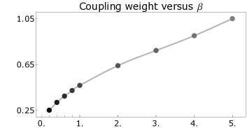
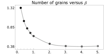
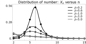
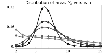
Figure 4: Self-similar solution for several values of $\beta$, where circles and lines represent numerical data and interpolating splines, respectively. Top row: $\Gamma$ and $\sum_{n=2}^{N}X_{n}$ versus $\beta$. Bottom row: $X_{n}$ and $Y_{n}$ versus $n$ with vertical line at $n=6$.

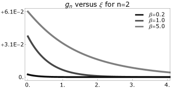
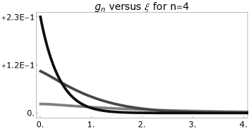
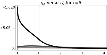
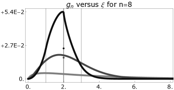
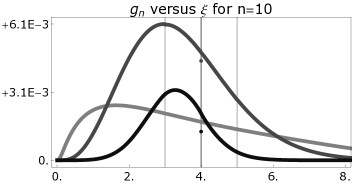
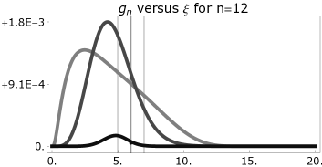
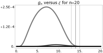
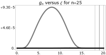
Figure 5: Plots of $g_{n}$ versus $\xi$ with vertical lines at $\xi=n-5$, $\xi=n-6$, and $\xi=n-7$. Notice that the plot range for $\xi$ varies with $n$.

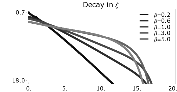
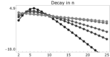
Figure 6: Decay of the solutions: $\ln{\big{(}\sum_{n=2}^{N}g_{n}{\left({\xi}\right)}\big{)}}$ versus $\xi$ and $\ln{X_{n}}$ versus $n$.

We performed a large number of numerical simulations for various values of $\beta$ and different types of initial values (random, uniformly distributed, and several variants of localized data). To ensure that the initial data belong in fact to the set $\mathcal{U}_{+}$, we chose at first nonnegative values $\tilde{g}_{n}^{k}$ for $n=2{...}{N-1}$ and $k=1{...}{K-1}$, and computed afterwards two scaling factors $\alpha_{1}$ and $\alpha_{2}$ such that $g_{n}^{k}={\left({\chi_{2\leq{n}\leq{5}}\alpha_{1}+\chi_{6\leq{n}\leq{N}}\alpha_{2}}\right)}\tilde{g}_{n}^{k}$ satisfy the constraint $P+{\varepsilon}{Q}=0$ and yield the prescribed area.

In our simulations we observed that all numerical solutions for a given value of $\beta$ converge, as $t\to\infty$, to the same steady state. We therefore conjecture, that for all $\beta$ and $N<\infty$ there exists a unique steady state that is moreover a global attractor for $\eqref{Eqn:System.N}$. It would be highly desirable to give a rigorous justification for this numerical observation, but even to prove the uniqueness of $\Gamma$ remains a challenging task. We also conjecture that for $N=\infty$ there is only one self-similar solution with fast decay in $\xi$, but emphasize that self-similar solutions with slow decay might exist as well. Such solutions exist in related mean-field models for coarsening that couple transport and coalescence [13], but cannot be detected by our approximation scheme.

The numerically computed steady states for several values of $\beta\in[0.2,\,5.0]$ are, along with some derived data, depicted in Figures 4, 5, and 6. All computations are performed with $A=1$, $N=25$, $L=20$, and ${\varepsilon}=0.05$, and due to the numerically computed residuals we expect that the discrete solutions $g_{n}^{k}$ resemble the limit profiles $g_{n}$ with $N=\infty$ very well. In particular, Figure 6 confirms that the self-similar profiles for $N=\infty$ decay exponentially in $\xi$.

Figure 5 illustrates that for $n\geq 7$ there is no pointwise convergence $g_{n}^{k}\xrightarrow{{\varepsilon}\to 0}g_{n}$ at the critical point $\xi=n-6$. In fact, at least for small $\beta$ and moderate values of $n$ we observe that the discrete data $g_{n}^{k_{n}}$ are considerably smaller than $g_{n}{\left({n-6}\right)}$. This phenomenon stems from our discretization and can be understood as follows. On the discrete level steady states satisfy, see (11),

$${\left({\Gamma\kappa_{n}-1}\right)}g_{n}^{k_{n}} =\Gamma{\left({\beta(n-1)g_{n-1}^{k_{n}}+{\left({\beta+1}\right)}{\left({n+1}\right)}g_{n+1}^{k_{n}}}\right)},$$

$${\left({\Gamma\kappa_{n}-1}\right)}g_{n}^{k_{n}\pm{1}}-g_{n}^{k_{n}\pm{2}} =\Gamma{\left({\beta(n-1)g_{n-1}^{k_{n}\pm{1}}+{\left({\beta+1}\right)}{\left({n+1}\right)}g_{n+1}^{k_{n}\pm{1}}}\right)}.$$

For small ${\varepsilon}$ we can express the right hand sides in terms of $g_{n\pm{1}}{\left({n-6}\right)}$, the values of the limit functions $g_{n\pm 1}$ at $\xi=n-6$. Equating the resulting right hand sides we then conclude that

$${\left({\Gamma\kappa_{n}-1}\right)}g_{n}^{k_{n}}={\left({\Gamma\kappa_{n}-1}\right)}g_{n}^{k_{n}\pm{1}}-g_{n}^{k_{n}\pm{2}}+{o{\left({1}\right)}}.$$

If the limit function $g_{n}$ is also continuous at $\xi=n-6$ (according to Lemma 19, this happens for $\Gamma>2/\kappa_{n}=2/(2\beta+1)n$ and hence at least for large $n$) we can approximate the terms $g_{n}^{k_{n}\pm 1}$ and $g_{n}^{k_{n}\pm 2}$ by $g_{n}{\left({n-6}\right)}$. This gives

$$g_{n}^{k_{n}}\quad\xrightarrow{{\varepsilon}\to 0}\quad\frac{\Gamma\kappa_{n}-2}{\Gamma\kappa_{n}-1}g_{n}{\left({n-6}\right)}={\left({1-\frac{1}{\Gamma{\left({2\beta+1}\right)}n-1}}\right)}g_{n}{\left({n-6}\right)},$$

where the right hand side is always nonnegative due to $g_{n}{\left({n-6}\right)}\geq 0$ and $\Gamma\kappa_{n}>2$.

Acknowledgements

We thank Francis Filbet for illuminating discussions and the Universities of Lyon 1, Oxford and Toulouse 3 for their hospitality.

References

- [1] H. Amann. Ordinary differential equations, volume 13 of de Gruyter Studies in Mathematics. Walter de Gruyter & Co., Berlin, 1990. An introduction to nonlinear analysis, Translated from the German by Gerhard Metzen.
- [2] M. P. Anderson, D. J. Srolovitz, G. S. Grest, and P. Sahni. Computer simulation of grain growth-I. Kinetics. Acta metall., 32:783–791, 1984.
- [3] M. P. Anderson, D. J. Srolovitz, G. S. Grest, and P. Sahni. Computer simulation of grain growth-II. Grain size distribution, topology, and local dynamics. Acta metall., 32:793–802, 1984.
- [4] K. Barmak, E. Eggeling, M. Emelianenko, Y. Epshteyn, D. Kinderlehrer, R. Sharp, and S. Ta’asan. Critical events, entropy, and the grain boundary character distribution. Phys. Rev. B, 83:134117, 2011.
- [5] K. Barmak, E. Eggeling, M. Emelianenko, Y. Epshteyn, D. Kinderlehrer, R. Sharp, and S. Ta’asan. An entropy based theory of the grain boundary character distribution. Discret. Contin. Dyn. Syst. - Ser. A, 30:427–454, 2011.
- [6] A. Cohen. A stochastic approach to coarsening of cellular networks. Multiscale Model. Simul., 8(2):463–480, 2009/10.
- [7] M. Elsey, S. Esedoglu, and P. Smereka. Diffusion generated motion for grain growth in two and three dimensions. J. Comput. Phys., 228:21:8015–8033, 2009.
- [8] M. Elsey, S. Esedoglu, and P. Smereka. Large scale simulation of normal grain growth via diffusion generated motion. Proc. R. Soc. A, 467:2126:381–401, 2011.
- [9] N. Fournier and Ph. Laurençot. Existence of self-similar solutions to Smoluchowski’s coagulation equation. Comm. Math. Phys., 256(3):589–609, 2005.
- [10] V. E. Fradkov. A theoretical investigation of two-dimensional grain growth in the ‘gas’ approximation. Phil. Mag. Lett., 58:271–275, 1988.
- [11] V. E. Fradkov and D. G. Udler. 2D normal grain growth: Topological aspects. Adv. Phys., 43:739–789, 1994.
- [12] R. Henseler, M. Herrmann, B. Niethammer, and Juan J.L. Velázquez. A kinetic model for grain growth. Kinet. Relat. Models, 1(4):591 – 617, 2008.
- [13] M. Herrmann, Ph. Laurençot, and B. Niethammer. Self-similar solutions for fat tails for a coagulation equation with nonlocal drift. C. R. Math. Acad. Sci. Paris, 347(15-16):909–914, 2009.
- [14] K. Kawasaki, T. Nagai, and K. Nakashima. Vertex models for two–dimensional grain growth. Phil. Mag. B, 60:399–421, 1989.
- [15] D. Kinderlehrer and C. Liu. Evolution of grain boundaries. Math. Models Methods Appl. Sci., 11:713–729, 2001.
- [16] C. Mantegazza, M. Novaga, and V. M. Tortorelli. Motion by curvature of planar networks. Ann. Sc. Norm. Super. Pisa Cl. Sci., 3:235–324, 2004.
- [17] W. W. Mullins. Two–dimensional motion of idealized grain boundaries. J. Appl. Phys., 27:900–904, 1956.