Modelling neutral hydrogen in galaxies using cosmological hydrodynamical simulations

Abstract

The characterisation of the atomic and molecular hydrogen content of high-redshift galaxies is a major observational challenge that will be addressed over the coming years with a new generation of radio telescopes. We investigate this important issue by considering the states of hydrogen across a range of structures within high-resolution cosmological hydrodynamical simulations. Additionally, our simulations allow us to investigate the sensitivity of our results to numerical resolution and to sub-grid baryonic physics (especially feedback from supernovae and active galactic nuclei). We find that the most significant uncertainty in modelling the neutral hydrogen distribution arises from our need to model a self-shielding correction in moderate density regions. Future simulations incorporating radiative transfer schemes will be vital to improve on our empirical self-shielding threshold. Irrespective of the exact nature of the threshold we find that while the atomic hydrogen mass function evolves only mildly from redshift two to zero, the molecular hydrogen mass function increases with increasing redshift, especially at the high-mass end. Interestingly, the weak evolution of the neutral hydrogen mass function is insensitive to the feedback scheme utilised, but the opposite is true for the molecular gas, which is more closely associated with the star formation in the simulations.

1 Introduction

Approximately 75 per cent of the baryonic material in the Universe is hydrogen, so understanding and being able to reproduce the distribution of its various phases is a crucial step in constructing a complete theory of galaxy formation. After re-ionisation completed at $z\simeq 6$, the majority of the hydrogen is expected to reside in a diffuse, ionised state outside of galaxies. However, it is also believed that significant reservoirs of neutral (atomic and molecular) hydrogen must exist, particularly at high-redshift, as this is the basic fuel for star formation.

At higher densities than the diffuse, ionised intergalactic medium surrounding the galaxies, large-scale gas clouds are visible in absorption as the Lyman-$\alpha$ forest. The latter can be probed by observations of intervening low column density HI structures in the spectra of quasars found, for example, in the Sloan Digital Sky Survey (e.g. Prochaska et al., 2010). As we probe ever closer to the galaxy disks the gas density increases, along with the HI surface density, allowing us to directly probe the emission from neutral hydrogen. While a challenging observation, it greatly expands our understanding of galaxy formation on scales at which the galaxies themselves reside. For these reasons, great efforts have been made in surveying the emission of HI in the local Universe, such as the HI Parkes All Sky Survey, HIPASS (Barnes et al., 2001; Meyer et al., 2004) and the HI Jodrell All Sky Survey, HIJASS (Lang et al., 2003). The currently ongoing Arecibo Legacy Fast ALFA survey, ALFALFA (Giovanelli et al., 2005), is producing the deepest all sky HI maps of the local Universe ever created (e.g. Martin et al., 2010).

The gas that resides inside the galaxy disk forms a multiphase medium in which HI gas forms $\rm H_{2}$ in the densest regions. The Atacama Large Millimeter Array (ALMA) promises to reveal an unprecedented wealth of information $\rm H_{2}$ an important tracer of star formation. Radiation from young stars which form in these regions give rise to ionised bubbles of HII, emitting intense Lyman-$\alpha$ radiation, notably surveyed in SINGS (Meurer et al., 2006).

In addition to these impressive surveys are equally impressive plans for next generation radio telescopes. For example Apertif, MeerKAT and ASKAP are the pathfinder missions for the ambitious Square Kilometer Array (SKA) which may detect $10^{9}$ galaxies out to $z\approx 1.5$ yielding strong cosmological constraints (Abdalla & Rawlings, 2005). The ASKAP all sky survey, WALLABY, will detect $5\times 10^{5}$ galaxies in HI (Duffy et al., 2011) which will be the largest catalogue until the completion of the Five hundred metre Array Spherical Telescope (FAST) which complements SKA in the Northern hemisphere, potentially detecting $10^{6}$ galaxies with mean redshift $\bar{z}\approx 0.15$ (Duffy et al., 2008).

Together these planned telescopes will revolutionise our ability to measure both the local HI mass function and its evolution to high redshifts, as well as the distribution of HI within galaxies across a large fraction of the Universe. The expected HI data is, however, far in advance of current theoretical models due to the intrinsic complications of HI formation and destruction in galaxies. This is in addition to the already uncertain gas treatment in the theoretical models for sub-grid baryonic physics.

Although the detailed distribution of HI is not well understood, the basic picture of the lifecycle of HI can be reasonably well described through simple physical arguments. The gravitational potential of the dark matter forms the framework in which gas can accumulate, cooling through a variety of thermal and non-thermal emission mechanisms. However, due to the cosmic UV background only haloes with a virial temperature greater than $\sim 10^{4}\,\rm K$ can retain this gas, thereby setting an effective lower mass floor for the haloes that can host galaxies (e.g. Quinn et al., 1996). Eventually, as the gas density increases, it can become self-shielded against this background UV flux and will form large collections of cold, neutral hydrogen. In the centres of these clouds molecular hydrogen may form which will lead to a rapid cooling of the gas. The dense core of clouds may then experience thermo-gravitational instabilities which can lead to star formation (Schaye, 2004). The high-mass stars will in turn ionise the very regions that helped create them. This is accomplished directly via photo-ionising radiation from the stars, as well as in driving bulk motions of the gas from the galaxy, in turn reducing the self-shielding against the background radiation field (e.g. Pawlik & Schaye, 2009).

In an ideal simulation one would trace the impact of individual stars, or stellar regions, in ionising the gas and thereby accurately track the non-local effects of star formation on the Interstellar Medium (ISM). This is an extremely computationally expensive process for the large number of galaxies formed in hydrodynamical simulations of cosmological volumes, such as is considered in this work. However, by limiting the radiative transfer scheme to postprocessing existing datasets, Altay et al. (2010) were able to accurately model the neutral hydrogen column density distribution function at $z=3$ (a separate study by McQuinn et al. (2011) was similarly successful using a postprocessing radiative transfer scheme at $z=3$). Altay et al. (2010) found that it was critical to model self-shielding above column densities of $10^{18}\rm\,cm^{-2}$ and molecular hydrogen formation above $10^{21.5}\rm\,cm^{-2}$. In particular we adopt their empirical treatment of molecular hydrogen formation at high gas densities as discussed in Section 3.2.

Several other works have studied the distribution of HI at $z=3$ such as Pontzen et al. (2008), Razoumov et al. (2008) and Tescari et al. (2009) but most relevant for our investigation of the low redshift Universe is Popping et al. (2009), henceforth P09. We argue that our higher resolution simulations allow us to make more realistic and better resolved predictions for the HI, H₂ and cold gas mass functions, extending this work to the evolution of the mass functions and investigate the sensitivity to the physics scheme incorporated; a significant improvement on all existing hydrodynamical studies to date.

Other works investigating HI in galaxies across cosmological scales have taken a semi-analytic approach, for example in Obreschkow et al. (2009) they calculated that the neutral hydrogen in galaxies was distributed across atomic and molecular states with a ratio, $R=M_{\rm H_{2}}/M_{\rm HI}$ that increased with the gas mass of the halo. Adopting this approach they found that semi-analytic models could reproduce the $z=0$ HI mass function above $M_{\rm HI}=10^{9}\,{\rm M_{\odot}}$, below this mass they found a factor two over abundance of galaxies relative to the observations. This was opposite to another semi-analytic study based on the same underlying DM simulation; in Power et al. (2010) it was noted that such low mass HI systems were too rare. Interestingly it has been suggested by Lagos et al. (2011) that if one were to split the cold gas into HI and H₂ during the simulation, rather than in postprocessing, and form stars based on the latter alone, then many more low mass HI systems survive in the simulations.

In Obreschkow & Rawlings (2009a) the ratio $R$ from Obreschkow et al. (2009) was applied at higher redshifts. With this scheme they found that there was little evolution in the cosmic density of HI in the Universe, $\Omega_{\rm HI}$, to $z=1$ beyond which the value dramatically decreased, with only half of the local HI predicted to exist in galaxies by $z=3$. This is in contrast to conclusions made on the basis of observations of damped Ly$\alpha$ systems (e.g. Prochaska et al., 2005; Rao et al., 2006) which infer a factor two increase by $z\approx 3$. Further observations from DLA systems (Prochaska & Wolfe, 2009) indicate that the comoving HI density at $z=2$ is, within the errors, consistent with the result at $z=0$ as measured by HIPASS (Zwaan et al., 2005) (with a best-fit value only $5\%$ higher). This local value is similar to the partly completed ALFALFA survey of the local Universe, although they find a value $16\%$ higher (Martin et al., 2010). Tantalising evidence that the HI cosmic density at $z=0.8$ is also similar to that at $z=0$ is given by Chang et al. (2010), who cross-correlated galaxies from optical catalogues with brightness temperature radio maps to measure a statistical ‘stacked’ estimate of the HI emission. Furthermore, Prochaska & Wolfe (2009) found that this value increases weakly beyond $z=1$, only doubling over the redshift range $z\approx 2\,-\,4$. Therefore, although the integrated HI mass function is observed to be roughly constant in time, the distribution of HI in mass may vary. This is the main subject of our work and the goal of upcoming deep radio surveys.

This paper is organised as follows. In Section 2 we describe the physics models and range of resolutions that we have simulated as well as the numerical tests we have performed to remove artefacts. In Section 3 we detail our methodology of converting the hydrogen abundances of the simulation into HII, HI, $\rm H_{2}$. We analyse the HI properties of haloes in Section 4. First we consider the distribution of the stellar mass and gaseous components as a function of halo mass in Section 4.2. We then probe the HI and $\rm H_{2}$ as a function of stellar mass in Section 4.3. As a last probe of the distribution of the baryons within haloes we examine their half-mass radii for various halo masses and redshifts in Section 4.4. We then consider the HI and $\rm H_{2}$ mass functions and their evolution with redshift in Section 5. In Section 6 we vary the sub-grid physics schemes to probe the sensitivity of the mass function predictions to the particular physics prescription. Finally, we conclude in Section 7.

2 Simulation Details

We have made use of a number of high resolution, large-volume hydrodynamical runs created as part of the OverWhelmingly Large Simulations project (OWLS; Schaye et al. 2010). This series of simulations all share the same initial conditions, i.e. are identical simulation volumes, but are resimulated using $\sim 50$ different physics models which allows robust testing of the relative importance of each scheme. OWLS has seen a number of successes in reproducing observed galaxy properties. For example, the cosmic star formation history (e.g. Madau et al., 1996) was shown to be reproduced in Schaye et al. (2010). In Booth & Schaye (2009) and Booth & Schaye (2010) the AGN implementation was found to recover a number of empirical properties of super-massive black holes, such as the black hole mass - halo mass relation (Bandara et al., 2009); the black hole mass - stellar mass relation (e.g. Häring & Rix, 2004); and the black hole mass - bulge velocity dispersion correlation (e.g. Tremaine et al., 2002). Furthermore, this AGN implementation is capable of reproducing a number of galaxy group properties such as their X-ray temperature and density profiles as well as galaxy stellar masses and age distributions (McCarthy et al., 2010). Of particular note for this work is the study by Altay et al. (2010) who found that OWLS can reproduce the observed $z=3$ HI column density distribution function, when post-processed with a radiative transfer model. More generally, a particular strength of the OWLS suite is that the variety of models allows us to test the sensitivity of a particular observable phenomenon to the details of the physical processes included (e.g. metal enrichment, feedback mechanisms etc).

The OWLS simulations were run with an updated version of the publicly-available gadget-2 $N$-body/hydrodynamics code (Springel, 2005) with new modules for radiative cooling (Wiersma et al., 2009), star formation (Schaye & Dalla Vecchia, 2008), stellar evolution and mass loss (Wiersma et al., 2009), galactic winds driven by SNe (Dalla Vecchia & Schaye, 2008) and, for one model, AGN (Booth & Schaye, 2009). Each simulation employed $N^{3}$ dark matter (DM) particles, and $N^{3}$ gas particles, where $N=128$, $256$ and $512$, within cubic volumes of comoving length, $L=25$, $50$ and $100\,h^{-1}{\rm Mpc}$. For all cases, glass-like cosmological initial conditions were generated at $z=127$ using the Zeldovich approximation and a transfer function generated using cmbfast (v. 4.1, Seljak & Zaldarriaga 1996).

Simulations with the smallest box were run to $z=2$ and the two larger volumes were simulated down to $z=0$. For the present study the complete range of box sizes exist for only one of the physics models, that termed ‘ZC_WFB’ in Duffy et al. (2010). Table 1 lists the available box sizes and other pertinent numerical parameters, including the Plummer-equivalent softening lengths and particle masses. (Note that the dark matter particles have a mass that is a factor $(1-f^{\rm univ}_{\rm b})/f^{\rm univ}_{\rm b}$ greater than the mass of the gas particles, where $f^{\rm univ}_{\rm b}=\Omega_{\rm b}/\Omega_{\rm m}$ is the Universal baryon fraction.)

We use the Wilkinson Microwave Anisotropy Probe 3 year results (Spergel et al., 2007), henceforth known as WMAP3, to set the cosmological parameters $[\Omega_{\rm m},$ $\Omega_{\rm b},$ $\Omega_{\Lambda},$ $h,$ $\sigma_{8},$ $n_{\rm s}]$ to [0.238, 0.0418, 0.762, 0.73, 0.74, 0.95] and $f^{\rm univ}_{\rm b}=0.176$. Although we use a cosmology that has a $\sigma_{8}$ about $10\%$ lower than the current year 7 WMAP result (Komatsu et al., 2011) we believe that the effects on our predictions for the various phases of hydrogen will be small. This is because only the high-mass end ($M\geq 10^{14}\,h^{-1}{\rm M_{\odot}}$) of the mass function is exponentially sensitive to a change in $\sigma_{8}$ whereas the majority of the HI signal in our simulations is due to lower mass DM haloes near the ‘knee’ at $M\approx 10^{12}\,h^{-1}{\rm M_{\odot}}$ which are much less sensitive to $\sigma_{8}$. When comparing DM only simulations with $\sigma_{8}$ values for WMAP3 and 7, the overall number counts agree within 5 per cent for haloes of mass $M=10^{11}-10^{12}\,h^{-1}{\rm M_{\odot}}$, while clusters ($M=10^{14}-10^{15}\,h^{-1}{\rm M_{\odot}}$) are nearly 70 per cent more common in the higher $\sigma_{8}$ universe. We note that the study of the dependence of the hydrogen phases on the sub-grid physics will be insensitive to the cosmology used, as all simulations have the same initial conditions.

Table 1: Details of the various simulation parameters used in this study. From left to right the columns show: simulation identifier; the physics scheme(s) available; comoving box-size; number of dark matter particles (there are equally many baryonic particles); initial baryonic particle mass; dark matter particle mass; comoving (Plummer-equivalent) gravitational softening; maximum physical softening; final redshift. Note that we have adapted the OWLS simulation list from Schaye et al. (2010) such that REF in that work is referred to as ZC_WFB here, while All corresponds to the full range of simulations listed in Table 2.

Simulation	Physics	$L$	$N$	$m_{\rm b}$	$m_{\rm dm}$	$\epsilon_{\rm com}$	$\epsilon_{\rm prop}$	$z_{\rm end}$
		$(\,h^{-1}{\rm Mpc})$		$(\,h^{-1}{\rm M_{\odot}})$	$(\,h^{-1}{\rm M_{\odot}})$	$(\,h^{-1}{\rm kpc})$	$(\,h^{-1}{\rm kpc})$
L025N128	ZC_WFB	25	$128^{3}$	$8.7\times 10^{7}$	$4.1\times 10^{8}$	7.81	2.0	0
L025N256	ZC_WFB	25	$256^{3}$	$1.1\times 10^{7}$	$5.1\times 10^{7}$	3.91	1.0	2
L025N512	All	25	$512^{3}$	$1.4\times 10^{6}$	$6.3\times 10^{6}$	1.95	0.5	1.45
L050N128	ZC_WFB	50	$128^{3}$	$6.9\times 10^{8}$	$3.2\times 10^{9}$	15.62	4.0	0
L050N256	ZC_WFB	50	$256^{3}$	$8.7\times 10^{7}$	$4.1\times 10^{8}$	7.81	2.0	0
L050N512	All	50	$512^{3}$	$1.1\times 10^{7}$	$5.1\times 10^{7}$	3.91	1.0	0
L100N256	ZC_WFB	100	$256^{3}$	$6.9\times 10^{8}$	$3.2\times 10^{9}$	15.62	4.0	0
L100N512	All	100	$512^{3}$	$8.7\times 10^{7}$	$4.1\times 10^{8}$	7.81	2.0	0

2.1 Simulation models

We briefly recap the physics prescriptions used in this work but direct the reader to Schaye et al. (2010) and the references therein for a more extensive explanation. We are primarily interested in the sensitivity of the HI abundance to differing feedback schemes and identify such simulations with the labels ‘WFB’, ‘SFB’ or ‘NFB’ to denote stellar feedback that is weak, strong or absent, respectively. Furthermore we denote a simulation that includes AGN feedback by ‘AGN’. Lastly, we want to test the sensitivity of the results to the additional cooling of the gas due to the presence of metals and denote these simulations with ‘ZC’, while those without are labeled ‘PrimC’. Refer to Table 2 for an overview.

For the simulations labeled ‘PrimC’ we model the cooling of gas via line emission from primordial elements, H and He. Those labeled ‘ZC’ have additional contributions from nine metals: C, N, O, Ne, Mg, Si, S, Ca and Fe. In both cases, additional cooling via free-free Bremsstrahlung emission is also present. The cooling rates for the different elements are taken from 3-D cloudy (Ferland et al., 1998) tables which assume collisional equilibrium before reionisation ($z>9$) and photoionisaton equilibrium afterwards, due to the presence of an evolving meta-galactic UV/X-ray background (Haardt & Madau, 2001). For more details of the implementation of gas cooling (and heating) rates in the simulations, see Wiersma et al. (2009).

Gas particles are converted stochastically into stellar particles (such that particle numbers are conserved) at a pressure-dependent rate in accordance with the Kennicutt-Schmidt law (for a review see Kennicutt 1998) using the prescriptions of Schaye & Dalla Vecchia (2008). We assume a Chabrier initial mass function (IMF; see Chabrier 2003) within each star particle and track the metal mass released by the stars using the method described in Wiersma et al. (2009).

The stars formed in the simulations inject energy in neighbouring gas particles via kinetic feedback. For our assumed IMF, the energy per solar mass of material available from supernovae (SNe) is $1.8\times 10^{49}\,{\rm erg}\,{\rm M}^{-1}_{\odot}$. This is distributed amongst the local gas according to the dimensionless mass-loading parameter $\eta$, in which a total gas mass of $\eta{M}_{\rm SN}$ is given an initial wind velocity of ${v_{\rm w}}$. This results in a fraction

$$f_{w}\approx 0.4\left(\frac{\eta}{2}\right)\left(\frac{v_{\rm w}}{600\,{\rm km\,s^{-1}}}\right)^{2}\left(\frac{\epsilon_{\rm SN}}{1.8\times 10^{49}\,{\rm erg}\,{\rm M}^{-1}_{\odot}}\right)\,,$$ (1)

of the energy of the SNe being imparted in the form of kinetic feedback (Dalla Vecchia & Schaye, 2008); the values $\eta=2$ and $v_{\rm w}=600\,{\rm km\,s}^{-1}$ were adopted for the ‘WFB’ model. For the ‘SFB’ simulations $v_{\rm w}$ ($\eta$) increases (decreases) with the gas density in the region of the star while keeping $f_{w}$ fixed. Note that the kinetically-heated gas particles are never decoupled from the hydrodynamics and therefore will tend to collide and ‘drag’ a larger number of gas particles with them, resulting in an effective mass loading which is higher than implied by $\eta$.

In the simulations labeled ‘AGN’ the black hole at the centre of a halo grows at the expense of the surrounding gaseous medium by gas accretion as well as through mergers between black holes. The maximum accretion rate is capped at the Eddington limit and 1.5% of the rest mass energy of the accreted matter is distributed thermally to the nearby gas particles as explained in Booth & Schaye (2009). Booth & Schaye (2009) demonstrated that for this value of the feedback efficiency the observed scaling relations for supermassive black holes are reproduced.

Table 2: A list of the simulated sub-grid baryon physics schemes utilised in this study. From left to right, the columns list the simulation name used in this study; the name as defined by Schaye et al. (2010); and a brief the description of the physics modelled. The list of available simulations run with each model (box-size and resolution) is given in Table 1.

Simulation	OWLS name	Brief description
PrimC_NFB	NOSN_NOZCOOL	No energy feedback from SNe and cooling assumes primordial abundances
PrimC_WFB	NOZCOOL	Cooling as PrimC_NFB but with fixed mass loading of winds from SNe feedback
ZC_WFB	REF	SNe feedback as PrimC_WFB but now cooling rates include metal-line emission
ZC_SFB	WDENS	As ZC_WFB but wind mass loading and velocity depend on gas density
ZC_WFB_AGN	AGN	As ZC_WFB but with AGN feedback

2.2 Identifying Galaxies and Haloes

In this work we will consider the HI content of galaxies and the associated HI gas lying between them, which is particularly important in groups and clusters. We initially determine the halo in a simulation using a Friends-of-Friends (FoF) algorithm (Davis et al., 1985) with a linking length $b$. This will link all DM particles together that are within a distance $b\bar{l}$, where $\bar{l}$ is the mean inter-particle distance in the simulation. The gas is then attached to the nearest DM particle. The halo can thus have arbitrary shape, defined by an iso-density curve of overdensity relative to the background $\rho/\bar{\rho}\approx 3/(2\pi b^{3})$ (Cole & Lacey, 1996). We choose a value $b=0.2$ which, for an isothermal density profile, will have a halo mean over-density of $\langle\rho\rangle/\bar{\rho}\approx 180$ (Lacey & Cole, 1994). This is close to the spherical top-hat collapse model prediction for a virialised object $\approx 18\pi^{2}\approx 178$.

In the simulations with $L=100\,h^{-1}{\rm Mpc}$ we typically resolve 230 (15) haloes of virial mass $10^{13}-10^{14}\,h^{-1}{\rm M_{\odot}}$ ($>10^{14}\,h^{-1}{\rm M_{\odot}}$) at $z=0$ and for $L=25\,h^{-1}{\rm Mpc}$ there are 840 (13) haloes of $10^{12}-10^{13}\,h^{-1}{\rm M_{\odot}}$ ($>10^{13}\,h^{-1}{\rm M_{\odot}}$) at $z=2$. As all simulations of the same volume share the same initial conditions, the haloes formed are identical, except for the specific choice of sub-grid baryonic physics. This means that the number of haloes between simulations typically differs by less than 5 per cent, essentially due to slight variations in mass of specific haloes which can affect whether they meet mass cuts or not.

To identify gravitationally bound structures within haloes we use subfind (Dolag et al., 2009). This allows us, for example, to identify gas that has been stripped from an infalling galaxy but which is still bound to the background cluster, as well as satellite galaxies. Unless stated otherwise, the masses and sizes which we will quote are for objects found with subfind (and we will refer to such objects as galaxies), but when we discuss the halo in full (including satellites) we will use that which comes from the FoF algorithm and will add the ‘Halo’ superscript to the variable.

3 Modelling the Neutral Hydrogen

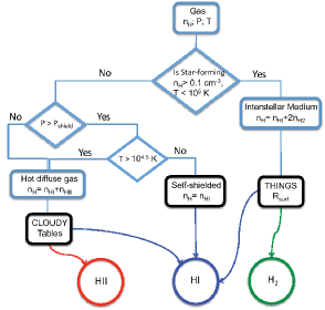
Figure 1: A simple flow diagram indicating the methodology to attribute the states of hydrogen to the gas particles of the simulation. In our model, the HII and $\rm H_{2}$ components arise from the diffuse (intergalactic) and star-forming (interstellar) components respectively, whereas the HI signal is found in all regimes. Note that we only ever consider particles that belong to gravitationally bound structure.

In this section we discuss our method for calculating the mass fraction of hydrogen in neutral molecular (H₂), atomic (HI) and ionised (HII) phases, for each gas particle. The total hydrogen mass fraction is first estimated for each particle by taking a smoothed average over its neighbours, using the SPH kernel (a value for the hydrogen abundance is carried by individual particles). The methodology for splitting the gas into the 3 phases of hydrogen depends on whether it is low-density intergalactic gas or high-density interstellar gas. We consider each one in turn below, with the overall procedure summarised as a flow diagram in Fig. 1.

3.1 Intergalactic Gas

Most of the gas resides outside, or in the outskirts, of galaxies and will have a significant HII component, due to both the photo-ionising UV/X-ray background and collisional ionisation resulting from gravitational shock heating. OWLS tracks an evolving UV/X-ray background (Haardt & Madau, 2001) after reionisation at $z=9$, that primarily affects the cold, low-density intergalactic medium. Gas at higher density can cool more efficiently, leading to larger neutral (HI) fractions (for full details see Wiersma et al. 2009). A significant fraction of gas is shock-heated to much higher temperatures at low-redshift, creating the warm-hot intergalactic medium and the intracluster medium. We use pre-calculated ionisation tables for hydrogen from cloudy (Ferland et al., 1998), to compute the optically thin HI and HII fractions of gas particles as a function of their current temperature and (SPH smoothed) density.

3.1.1 Optically Thick Gas

For gas that resides at moderate densities (in the range $n_{\rm H}\approx 10^{-4}\,-\,10^{-1}\,{\rm cm^{-3}}$) assumptions of optically thin gas exposed to a uniform UV background start to break down. Firstly, the local galactic UV intensity can be significantly stronger than the global average, from the presence of young massive stars or a quasar (the so-called proximity effect). In this case, the CLOUDY tables will overestimate the amount of HI present as the assumed photo-ionisation rate will be lower than it should be. Secondly, near galaxies the gas density can reach levels which are sufficient to self-shield the gas from the global UV background, which in turn would lead us to underestimate the fraction of HI. As we have previously discussed, ideally we would perform a full radiative transfer calculation to distribute ionising flux from nearby stellar sources through the gas. Such a technique would also lead to a more realistic calculation of the self-shielding in dense regions. We turn to simpler prescriptions that can be more easily applied to large volume simulations. In this study, we assume that only the self-shielding is important and attempt to correct for it using a simple method guided by the observational data.

3.1.2 Self-shielding Correction

We follow a methodology similar to that of P09 and choose to approximate the onset of self-shielding by adopting a pressure-based threshold. It is reasonable to expect that self-shielding occurs above a given surface density. As, shown by e.g. Schaye & Dalla Vecchia (2008), the pressure in the disk ought to scale quadratically with the surface density as the thickness of the disk is set by the local Jeans length. We can even use similar arguments to define an order of magnitude estimate for the pressure threshold value $P_{\rm shield}$ by considering the local volume density at the threshold, $n_{\rm shield}$, related to the pressure by $P_{\rm shield}/k=(n_{\rm shield}/k)10^{4}\,\rm K$ with a calculation of $n_{\rm shield}$ from Equation 11 in Schaye (2001b)

$$n_{\rm H,\,shield} = 10^{-4}{\,\rm cm^{-3}}(1+\delta)^{-1.5}\Gamma\left(\frac{T}{10^{4}\,\rm K}\right)^{-1}$$ (2)

$$\times\left(\frac{1+z}{4}\right)^{-9/2}\left(\frac{\Omega_{\rm b}h^{2}}{0.02}\right)^{-3/2}\left(\frac{f_{\rm g}}{0.16}\right)^{-1/2}$$

$$\times\frac{N_{\rm HI}}{2.7\times 10^{13}{\,\rm cm^{-2}}}\,,$$

giving $n_{\rm H,\,shield}\simeq 10^{-3}-10^{-2}\,\rm cm^{-3}$ for $z=3$ and assuming that overdensities relative to the background density, $\delta$, of order $10^{2}$ represent self-shielded galaxies, which have a fraction $f_{\rm g}$ of their disk mass in HI. This is equivalent to a pressure $P_{\rm shield}/k\simeq 10-10^{2}\,\rm Kcm^{-3}$. This simple estimate has been confirmed using a radiative transfer simulation in Altay et al. (2010).

The pressure threshold used in P09 was tuned to reproduce the mean HI density from the 1000 Brightest HIPASS galaxy catalogue (Zwaan et al., 2003), finding a value $P_{\rm shield}/k=155\,\rm Kcm^{-3}$. They only applied this to gas cool (or dense) enough to have a recombination time less than or equal to the sound crossing time (see Fig. 2 in P09). While it is clear that hot, collisionally ionised gas should be excluded, the physical motivation for the particular criterion chosen by P09 is unclear to us. We simply use an upper temperature limit for gas that is considered to be self-shielded, essentially forming a ‘cold’ gas population with $T\leq 10^{4.5}\,\rm K$. Our approach is similar to that adopted by Power et al. (2010) for their investigation of cold ($T\leq 10^{4}\,\rm K$) gas mass functions from semi-analytic simulations.

Table 3: A list of the pressure thresholds used to approximate the onset of self-shielding, $P_{\rm shield}/k$, for gas particles that have temperatures below $10^{4.5}\,\rm K$ in methods $\rm SS_{ALFALFA}$ (2nd column, normalised to low-redshift ALFALFA observations) and $\rm SS_{DLA}$ (3rd column, normalised to high-redshift Damped Lyman-$\alpha$ observations). Values in brackets denote pressure thresholds that produce HI densities 10 per cent higher and lower than observed, respectively. Zero values correspond to cases where even making all cold gas in the galaxy neutral gives insufficient HI to match the observations (typically $\sim$ 20 per cent below the desired value). The neutral interstellar gas is still separated into atomic and molecular neutral components.

Simulation	$\rm SS_{ALFALFA}$	$\rm SS_{DLA}$
PrimC_NFB	0 [0, 0]	159 [132, 193]
PrimC_WFB	0 [0, 0]	47 [30, 68]
ZC_WFB	150 [133,175]	98 [80, 123]
ZC_SFB	74 [60, 93]	17 [3, 28]
ZC_WFB_AGN	27 [21, 35]	76 [62, 93]

In what follows we have treated the self-shielding regime in three different ways. In what we shall call $\rm SS_{None}$ we shall presume that there is no self-shielding. This is clearly unphysical but it can be helpful to compare this with the other two methods. For method $\rm SS_{ALFALFA}$ we match the measured cosmic HI density in the HI mass range, $M_{\rm HI}=10^{10}-10^{11}\,h^{-1}{\rm M_{\odot}}$, from the $z=0$ ALFALFA survey (Martin et al., 2010). This normalisation is computed for the $100\,h^{-1}{\rm Mpc}$ simulation as this volume has been run with all sub-grid physics models. Cold gas above the pressure limit is then considered to be completely neutral, while gas below the threshold has HI and HII fractions taken from the optically-thin cloudy tables discussed previously. We find that a pressure of $P_{\rm shield}/k\approx 150\,\rm Kcm^{-3}$ matches the ALFALFA result for our default model (ZC_WFB, which is also the simulation closest to that studied by P09 in terms of the sub-grid physics modelled). The pressure thresholds used for all simulation models are listed in Table 3; typically in runs with stronger feedback we require a lower pressure threshold to match the HI density while in the runs with primordial cooling and weak or no feedback, there is insufficient ($\sim$ 20 per cent too low) HI gas in simulated galaxies to match the observations at low-redshift (the reverse is true at high-redshift).

There is no reason to believe that the pressure threshold will be independent of redshift. In fact, we expect it to depend on the intensity of the evolving UV background (Schaye, 2001b). For method $\rm SS_{DLA}$ we therefore normalise $P_{\rm shield}$ to agree with observations at higher redshift, namely the cosmic HI density inferred from Damped Lyman-$\alpha$ absorption systems. In particular, we will use measurements presented in Prochaska & Wolfe (2009) for $z\approx 2$. These results are close to the $z=0$ HI cosmic density inferred by ALFALFA (e.g. $\Omega_{\rm HI,DLA}=1.05\,\Omega_{\rm HI,ALFALFA}=3.75\times 10^{-4}$), but lead to somewhat higher values for $P_{\rm shield}$. We tune the pressure value until the integrated HI mass function (where available, as shown in Fig. 11) matches $\Omega_{\rm HI,DLA}$.

3.2 Star-forming Interstellar gas

As gas cools, its density will eventually increase until its structure can no longer be modelled reliably in our simulations. Such gas, associated with the star-forming interstellar medium in galaxies, is expected to be multiphase for hydrogen particle number densities above ${n}^{*}_{\rm H}\approx 10^{-2}$ - $10^{-1}\,{\rm cm}^{-3}$ (Schaye, 2004). In OWLS, such gas particles are identified when they exceed a critical particle density, ${n}^{*}_{\rm H}=0.1\,{\rm cm}^{-3}$ and have a temperature smaller than $10^{5}\,\rm K$, after which the gas density and pressure is evolved according to an effective polytropic Equation of state

$$P=P_{\rm crit}\left(\frac{n_{\rm H}}{{n}^{*}_{\rm H}}\right)^{\gamma_{\rm eff}}\,,$$ (3)

where $P_{\rm crit}/k=2.3\times 10^{3}\,{\rm K}\,{\rm cm}^{-3}$. All runs considered assume $\gamma_{\rm eff}=4/3$ which has the advantage that the Jeans mass is independent of density (Schaye & Dalla Vecchia, 2008), avoiding the situation where particle masses are greater than the Jeans mass in dense regions, a numerical artefact known to result in artificial fragmentation of the gas cloud (Bate & Burkert, 1997).

The Equation of state gas, which we will refer to as interstellar gas, lies in dense regions of the simulation where self-shielding effects are important. We therefore assume that the hydrogen exists as either HI or $\rm H_{2}$ (we ignore interstellar HII regions as they will contribute little to the hydrogen mass in galaxies). To separate the two phases, we utilise the empirical ratio relating $\rm H_{2}$ and HI surface densities, $R_{\rm surf}=\Sigma_{\rm H_{2}}/\Sigma_{\rm HI}$, to the local ISM pressure measured in the THINGS survey (Table 6 and Fig. 17 of Leroy et al. 2008), given by

$$R_{\rm surf}=\left(\frac{P/k}{10^{4.23}\,{\rm Kcm^{-3}}}\right)^{0.8}\,,$$ (4)

which was observed for a pressure range of $10^{3}\leq P/k\,[\rm K\,cm^{-3}]\leq 10^{6}$. It is then a trivial step to compute the mass of interstellar gas in atomic HI,

$${M_{\rm HI}}={M_{\rm H}}/(1+R_{\rm surf})\,.$$ (5)

Note that we have assumed that the HI and H₂ in the same disk are measured locally.

In using Equation 5 we must consider whether the pressure used in the empirical law of Equation 4 corresponds to the pressure averaged over the physical length scales that the simulations resolve. The THINGS survey reduces its sample of 23 dwarf and gas spiral galaxies to a standard resolution of $\sim 20$ arc seconds. However, the dwarf galaxies are typically closer than the spirals, as they are less luminous. The resolved physical lengthscales for the dwarf and spiral galaxies are around 400 and 800 pc respectively. This is close to the Plummer-equivalent softening length-scale (in proper units) of the $N=512^{3}$ simulations, as given in Table 1. Only the $100\,h^{-1}\,{\rm Mpc}$ boxsize may be cause for concern when we convert the pressure to HI mass, but as shown in Appendix A.1, this simulation appears sufficiently well resolved.

We also note that Equation 4 is for the local Universe only and the assumption that it holds at higher redshifts is potentially an issue. It is believed that this ratio will depend on metallicity (Schaye, 2001a, 2004; Krumholz et al., 2008, 2009) which decreases with redshift (e.g. Tremonti et al., 2004; Savaglio et al., 2005; Erb et al., 2006). We therefore caution the reader that the molecular fraction is likely to be a more complicated function of galactic properties than assumed here, given the limited physical information we have for galaxies in our simulations.

3.3 Resultant phase diagram for a specific case

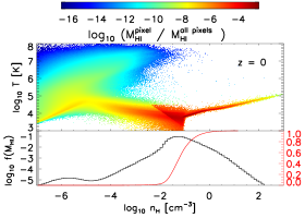
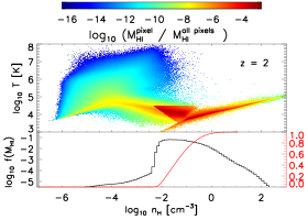
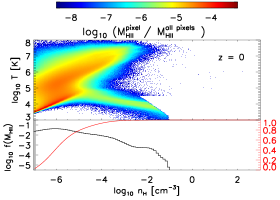
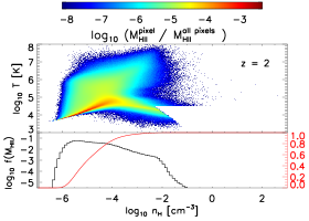
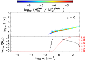
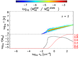
Figure 2: From top to bottom, we present the mass fraction of HI, HII and $\rm H_{2}$ for all gas in a simulation for a given gas temperature and hydrogen particle number density, in the ZC_WFB simulation. Left panels show results at $z=0$ and right panels for $z=2$. Method $\rm SS_{ALFALFA}$ is assumed for the self-shielding correction (tuned to the ALFALFA HI mass function at low-redshift). Additionally, we have projected each fraction as a function of density in the histogram below each image (black line), with the red line a simple cumulative distribution function of this histogram. The pressure threshold for the onset of self-shielding is especially clear in the top panels as a discontinuity in the HI fraction. The $\rm H_{2}$ is constrained, by design, to reside in the high-pressure multiphase ISM, modelled as a polytropic Equation of state.

In Fig. 2 we show the overall neutral fraction in atomic (HI; top panel) and molecular ($\rm H_{2}$; bottom panel) states as well as the ionised HII component (middle panel) in the temperature - density phase diagram at $z=0$ and $2$ (left and right columns respectively) for all gas particles in a simulation. We show results from the ZC_WFB $100\,h^{-1}{\rm Mpc}$ simulation, using method $\rm SS_{ALFALFA}$ for the self-shielding correction. (The equivalent phase diagrams for the other simulation schemes are broadly similar.)

The main result from the top panels is that the majority of HI resides near the self-shielding limit, demonstrating the importance of such a correction. Furthermore, even though at $z=0$ the majority of hydrogen resides in the hot plume of intergalactic material (middle panels), this gas is typically too highly ionised to be a large contributor to the overall HI mass. By design, the molecular component exists only in the densest material, which obeys the imposed Equation of state power law. Differences in the phases between low and high redshift are most apparent in the HI distribution below the self-shielding limit. At $z=2$ (right column) the HI content of the gas drops more sharply as the more intense global UV background ionises more of the gas.

The relative importance of each phase in gravitationally bound structure (and overall in the Universe) is summarised in Table 4 as a function of redshift for the $50\,h^{-1}{\rm Mpc}$ simulation with the ZC_WFB physics scheme and $\rm SS_{ALFALFA}$ self-shielding model.

Table 4: A list of relative fractions of the hydrogen phases (HII, HI and H₂) for the simulation model ZC_WFB in the $50\,h^{-1}{\rm Mpc}$ simulation volume using self-shielding threshold $\rm SS_{ALFALFA}$. As we are unable to resolve the low mass end of the galaxy distribution the HI and H₂ values are lower estimates. We consider the two cases for the hydrogen phases in both gravitationally bound structures and overall in the Universe (latter values are in parentheses).

Redshift	HII	HI	H2
0	0.964 (0.993)	0.026 (0.005)	0.010 (0.002)
1	0.862 (0.983)	0.085 (0.010)	0.053 (0.007)
2	0.736 (0.974)	0.167 (0.016)	0.097 (0.010)

4 Neutral Gas in Galaxies and Haloes

OWLS provides a wide range in dynamical mass over which the distribution of baryons can be measured. Additionally, different feedback and cooling schemes can be tested (e.g. Schaye et al., 2010; Duffy et al., 2010). In considering how the HII, HI and $\rm H_{2}$, as well as the stars formed from the dense hydrogen gas, are distributed across the simulation, we must separate the intertwined effects of baryon physics with mass scales and evolution. The results in this section concentrate on one simulation, ZC_WFB, but we will also make comparisons with ZC_WFB_AGN (arguably our most realistic model) to understand the possible effects of AGN feedback on the phases of hydrogen.

	$M_{\rm vir}=10^{12}\,h^{-1}{\rm M_{\odot}},\,z=2$	$M_{\rm vir}=10^{13}\,h^{-1}{\rm M_{\odot}},\,z=0$	$M_{\rm vir}=10^{14}\,h^{-1}{\rm M_{\odot}},\,z=0$
HII
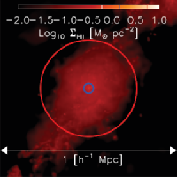
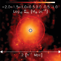
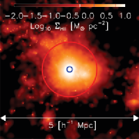
HI
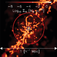
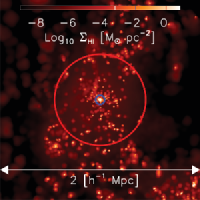
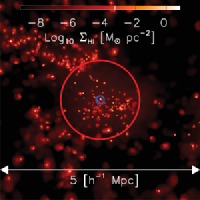
H2
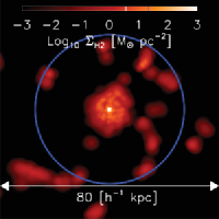
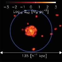
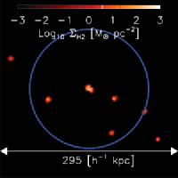
Stars

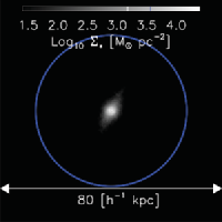
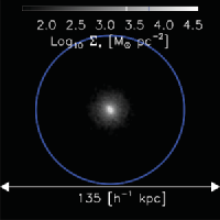
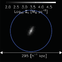
Figure 3: The distribution of various baryonic components in a typical $z=2$ galaxy (left), $z=0$ group (middle) and $z=0$ cluster halo (right), with $M_{\rm vir}\approx 10^{12}$, $10^{13}$ and $10^{14}\,h^{-1}{\rm M_{\odot}}$ respectively. We show the column densities of different baryonic components in the rows; from top to bottom these are HII, HI, $\rm H_{2}$ and stars. Results are taken from the $N=512$ simulation with $L=25$, $50$ and $100\,h^{-1}{\rm Mpc}$, left to right columns respectively. Note that different panels show different size regions, as indicated in each panel. The coordinates (column densities) are in comoving (proper) units. Red and blue circles denotes $R_{\rm vir}$ and $0.1\,R_{\rm vir}$, respectively. The boxes have the same length along the line of sight as across, as indicated by the arrow. All images have been rotated to present the object within $0.1\,R_{\rm vir}$ to be face-on.

In Fig. 3 we provide a visual overview of the effects of halo mass and redshift on the various distributions of the hydrogen phases. We compare haloes of virial mass $M_{\rm vir}\approx 10^{12}$, $10^{13}$ and $10^{14}\,h^{-1}{\rm M_{\odot}}$ (approximately corresponding to a galaxy, group and cluster, respectively), in columns left to right respectively. From top to bottom, the rows show density maps for the HII, HI, $\rm H_{2}$ and stellar components. The galaxy halo is at $z=2$ while the group and cluster haloes are at $z=0$.

Immediately apparent is the diffuse and filamentary nature of the HII in comparison with the clumpiness of the $\rm H_{2}$ / HI components, due to the latter two being associated with the cold and dense gas.

4.1 Resolution Effects

Before we study the neutral gas content of galaxies and haloes in detail, we first investigate the effects of resolution on our HI and H₂ mass determinations. This is presented in Appendix A where we test the effect of finite mass resolution and simulation box size on the predicted mass of HI (Appendix A.1), the HI mass function (Appendix A.2) and the molecular hydrogen mass function (Appendix A.3). In summary, we find that the properties of the baryonic species in haloes are converged above a certain limiting mass, with each species, X, as

$$M_{\rm res,\,X}=M_{\rm lim,\,X}\left(\frac{L}{50{\rm h^{-1}Mpc}}\frac{512}{N}\right)^{3}\,,$$ (6)

where $N$ is the cube-root of the number of Dark Matter particles and $L$ is the comoving length of the simulation cube. The co-efficient $M_{\rm lim}$ depends on the species X; in ascending mass order these are $M_{\rm lim}=[1,5,5,10,500]\times 10^{9}\,h^{-1}{\rm M_{\odot}}$ for X$=[{\rm HI},\,{\rm Cold\,Gas},\,{\rm Stellar},\,{\rm H_{2}},\,{\rm Virial}]$ respectively. This stellar mass limit implies that approximately 500 star particles are required for convergence, while the Virial (or Total) mass limit is dominated by the Dark Matter component and corresponds to nearly 7000 particles; from Duffy et al. (2010) we are confident that the masses and profiles of such systems are well converged. For HI, this value is more conservative than assumed by P09 who did not present convergence tests (see Fig. 15 for the comparison of the P09 results and our own resolution test).

4.2 Halo mass fractions

We now proceed to investigate the mass fractions of the various baryonic species in haloes. All available simulation volumes listed in Table 1 are used for the two sub-grid physics models considered, ZC_WFB and ZC_WFB_AGN. Taken together, we are able to probe a virial mass range of $5\times 10^{10}\,-\,5\times 10^{14}\,h^{-1}{\rm M_{\odot}}$, representing the largest dynamic range in mass yet considered in such a study. Such a large dynamic range allows us to probe whether there exists a characteristic mass scale at which HI is particularly abundant. This is an important issue for understanding the selection effects that a blind, flux-limited HI sample would suffer from, as well as the prospects of using HI surveys for cosmology. We only consider self-shielding method $\rm SS_{ALFALFA}$ in this section as we are primarily interested in the sensitivity of the various components to halo mass, redshift and galaxy formation modelling (specifically whether we include AGN or not).

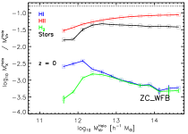
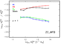
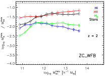
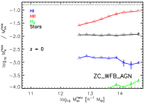
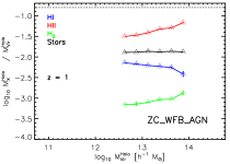
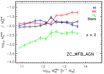
Figure 4: The HI, HII, $\rm H_{2}$ and stellar mass fractions of haloes as a function of the total halo mass for $z=0$, $1$ and $2$, left to right respectively. The horizontal dotted line is $0.9\,f^{\rm univ}_{\rm b}$, the value found in non-radiative gas simulations of Crain et al. (2007). We consider runs with metal line emission cooling and supernovae feedback, ZC_WFB, in the top row and then the runs with the AGN scheme added, ZC_WFB_AGN, in the bottom row. This latter case is particularly important when considering the stellar fractions in massive haloes. Method $\rm SS_{ALFALFA}$ (using ALFALFA data) is used for the self-shielding approximation. We only consider haloes with a virial mass above the limit in Equation 6, these haloes typically have $10^{4}$ dark matter particles. Note the smaller dynamic range in the AGN case at $z=0$ and 1 where we do not have an L050N12 simulation to probe galaxy scales.

In the top row of Fig. 4 we present the mass fraction of the baryonic species for ZC_WFB, as a function of halo mass at redshifts $z=0,1$ and 2 (left, middle and right panels, respectively). The bottom row shows the corresponding results for the simulation including AGN feedback (ZC_WFB_AGN).

At $z=0$ the ionised gas is the largest baryonic mass component of all haloes, followed by stars, although the two are comparable for $M_{\rm vir}\approx 10^{12}-10^{13}\,h^{-1}{\rm M_{\odot}}$. This pattern is seen at all redshifts both with and without AGN, although the ionised component is less dominant at higher redshifts.

For the simulation without AGN feedback (top row) the HI has a more complex distribution. At $z=0$, top left panel, there is an initial rise and then a clear decrease in the HI as a fraction of the total halo mass, beginning at $0.5$ percent at $M^{\rm Halo}_{\rm vir}\approx 10^{12}\,h^{-1}{\rm M_{\odot}}$ and decreasing to nearly an order of magnitude less at $M^{\rm Halo}_{\rm vir}\approx 5\times 10^{14}\,h^{-1}{\rm M_{\odot}}$. The pattern is similar at $z=2$ where the increased dynamic range allows us to identify a broader peak around a smaller mass, $M^{\rm Halo}_{\rm vir}\simeq 5\times 10^{11}\,h^{-1}{\rm M_{\odot}}$. However, at $z=2$ the HI mass fractions are typically an order of magnitude higher than at $z=0$. The $\rm H_{2}$ fractions broadly track the HI fractions although they are noticeably lower in the lowest mass haloes. In such systems, the mass fraction of baryons as a whole decreases as the gas is expelled by supernova feedback, leading to less efficient star formation. At higher masses (massive galaxies, groups and clusters) the decline in neutral fractions is due to the gas being used up and turned into stars, as the supernovae are no longer able to blow significant amounts of gas out of the halo. Ram pressure stripping of the cold gas in the hot halo atmospheres and the larger cooling times also contribute.

We also see evidence of a form of ‘downsizing’ (e.g. Pozzetti et al., 2003; Fontana et al., 2004; Drory et al., 2003, 2005) in the HI and $\rm H_{2}$ fractions as a function of redshift, which decrease faster for higher halo masses. We attribute this to a runaway conversion of this gas into stars for the ZC_WFB simulation, as it was noted in Duffy et al. (2010) that this particular physics scheme overproduces the stellar fraction in groups. This can be seen in the bottom panels of Fig. 4 where we include AGN which prevents the cooling flows, giving a low stellar (and cold gas) mass fraction. AGN feedback strongly suppresses the molecular mass fractions. The HI fraction, however, is typically slightly greater than in the simulation without AGN feedback. This is due to the cold gas typically being at lower density in the AGN model due to the stronger feedback.

4.3 Stars and Neutral Hydrogen

In Fig. 5 we show the HI mass as a function of the stellar mass of the galaxies in ZC_WFB at $z=0$, $1$ and $2$, top to bottom panels respectively. There is a clear positive correlation between the two parameters, namely that larger stellar mass systems also have more HI, as shown in the left column. We probe this correlation over approximately 2 decades of stellar mass at $z=2$.

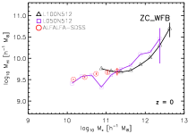
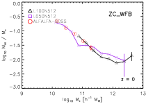
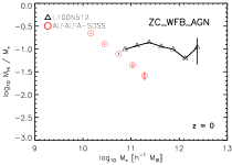
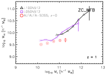
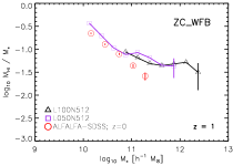
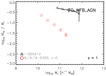
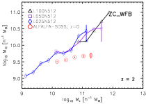
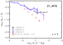
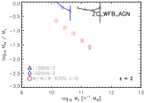
Figure 5: In the left column we present HI masses of all subhaloes in logarithmic bins of stellar mass $z=0$, $1$ and $2$, top to bottom respectively. The middle and right columns show the ratio of HI mass to stellar mass of each halo as a function of stellar mass. Results are for the ZC_WFB (left column) and the AGN model (right column, ZC_WFB_AGN). We have included a range of simulation volumes to attain the maximum dynamic range. We find that $5\times 10^{3}$ stellar particles is sufficient to attain a well resolved value. The errors are the $1\sigma$ errors estimated by bootstrap analysis and added in quadrature with Poisson error estimates (typically only important for the highest mass bins in a simulation). The red circles are from a joint ALFALFA-Sloan Digital Sky Survey comparison at low-redshift, compiled by Fabello et al. (2011), which nicely agree with our ZC_WFB simulation. Intriguingly the more realistic model which includes AGN overproduces the observed relation; to attain similar stellar masses the haloes with AGN are more massive. This also means that the haloes with have a higher HI mass as shown in Fig. 4.

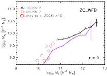
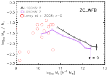
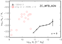
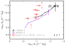
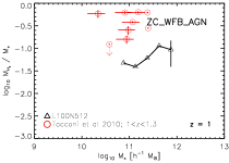
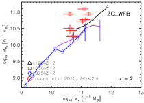
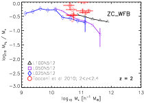
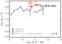
Figure 6: As in Fig. 5 but now we consider the molecular mass as a function of stellar mass in the objects for the ZC_WFB (left column) and the AGN model (right column, ZC_WFB_AGN). The errors are the $1\sigma$ errors estimated by bootstrap analysis and added in quadrature with Poisson error estimates (typically only important for the highest mass bins in a simulation). The red circles in the top row are local galaxies from Leroy et al. (2008) and at higher redshifts subsamples (close to the relevant redshift) from Tacconi et al. (2010).

The correlation seen in the left column of Fig. 5 is less than linear however, as is clear from the middle column where the ratio of HI to stellar mass is presented as a function of the stellar mass. The ratio is a decreasing function of stellar mass, which means that, for their size, massive galaxies are relatively deficient in HI when compared with smaller galaxies. This is in very good agreement with observations at low-redshift from Fabello et al. (2011), who combined HI and stellar data from the ALFALA and SDSS surveys, respectively (their results are plotted in Fig. 5 as red circles). We find that the trend continues at higher masses with the final data point indicating perhaps a turnover in the power law, a regime which is, however, influenced by the lack of AGN in this model. However, as seen in the right column of Fig. 5, model AGN typically has more HI at a given stellar mass than observed.

The ratio of HI to stellar mass increases with redshift. For example, at $z=2$ a galaxy of stellar mass $10^{11}\,h^{-1}{\rm M_{\odot}}$ will have nearly an order of magnitude more HI than a similar galaxy at the present day. Such an evolutionary trend is expected as the accretion of cold gas on to galaxies slows down with time and is no longer sufficient to replace the gas used in star formation (e.g. van de Voort et al., 2011a, b).

In Fig. 6 we consider the case of the molecular hydrogen as a function of the stellar mass of objects, for $z=0-2$ for a simulation with SNe feedback, and one with additional AGN feedback (ZC_WFB and ZC_WFB_AGN). For the former simulation at $z=0$ we compare to local galaxies from Leroy et al. (2008) we find that the simulations match the low stellar mass end well over the stellar mass range of the observations.

The situation at $z=2$ is more complex. At the low mass end the ZC_WFB simulation matches the observations of Tacconi et al. (2010), however for systems with stellar mass $\geq 10^{11}\,h^{-1}{\rm M_{\odot}}$ the observed galaxies typically have 0.5 dex greater molecular mass than the simulations. This situation becomes even more extreme at $z=1$ with the disparity at the high stellar mass end now an order of magnitude. We can attempt to match these observations by suppressing the conversion of cold gas into stars through additional feedback with an AGN but the discrepancy increases, with the molecular mass of simulated galaxies lying below the observations at all redshifts. If we compare this with the over-prediction of the HI mass for a given stellar mass (bottom right column of Fig. 5) we see that for a given stellar mass, the simulation with AGN feedback is probing haloes with a much greater halo mass and hence will have more shock-heated gas. In our formalism this will move gas from a dense regime in which it is dominated by molecular hydrogen into a lower density, hotter gas that has more atomic hydrogen, this redistribution of gas to larger radii is demonstrated in Fig. 7.

4.4 Spatial distributions

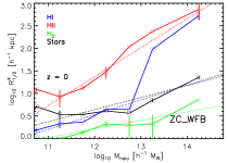
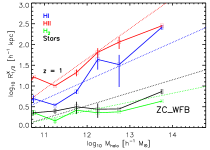
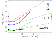
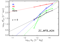
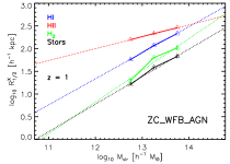
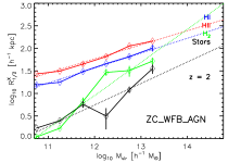
Figure 7: The HI, HII, $\rm H_{2}$ and stellar half-mass radii (in proper units) as a function of halo mass for $z=0$, $1$ and $2$, left to right respectively. We consider runs with metal-line cooling and supernovae feedback, ZC_WFB in the top row and also with the addition of AGN in ZC_WFB_AGN in the bottom row. Power law fits to all radii-mass relations are shown, with best-fit values given in Table 5.

As well as the total mass of each species in a given halo, we can probe the spatial distribution of the gas and stars within the haloes, as shown in Fig. 3. To quantify this Fig. 7 shows the half-mass radius for each species, $R^{\rm X}_{1/2}$, plotted as a function of halo mass for the different redshifts. Note that we only include particles that are gravitationally bound to the halo. Again, results are shown for the ZC_WFB runs.

In haloes more massive than $\sim 10^{13}\,h^{-1}{\rm M_{\odot}}$, the HI distribution rapidly becomes more extended than both the stellar and molecular H₂ distributions, growing to nearly half the size of the ionised diffuse component for haloes of mass $10^{14}\,h^{-1}{\rm M_{\odot}}$. Since the molecular gas is only identified with the high-density star-forming gas, it is not surprising that it has a similar half-mass radius as the stars (large differences start to appear in low-redshift groups and clusters due to the presence of a diffuse stellar component).

Table 5: Power-law fits to the half-mass radius versus halo mass relation for the various baryonic components given by $\log_{10}(R^{\rm X}_{1/2}/\,h^{-1}{\rm kpc})={\rm Norm}+{\rm Slope}\times\log_{10}(M_{\rm halo}/M_{\rm pivot})$ with a pivot mass of $2\times 10^{12}\,h^{-1}{\rm M_{\odot}}$ assumed. Quoted errors are 68 per cent confidence limits, estimated from bootstrap resampling. The top series of values are for ZC_WFB and the bottom set of three redshifts is for ZC_WFB_AGN.

$z$	HI		HII		$\rm H_{2}$		Stellar
	Norm [$\,h^{-1}{\rm kpc}$]	Ind	Norm [$\,h^{-1}{\rm kpc}$]	Ind	Norm [$\,h^{-1}{\rm kpc}$]	Ind	Norm [$\,h^{-1}{\rm kpc}$]	Ind
$0$	$10.31\pm^{0.43}_{0.39}$	$0.78\pm^{0.02}_{0.02}$	$165.96\pm^{0.83}_{0.95}$	$0.26\pm^{0.01}_{0.00}$	$2.39\pm^{0.11}_{0.10}$	$-0.06\pm^{0.04}_{0.10}$	$3.79\pm^{0.07}_{0.07}$	$0.25\pm^{0.01}_{0.01}$
$1$	$18.15\pm^{0.55}_{0.53}$	$0.74\pm^{0.01}_{0.01}$	$93.34\pm^{0.55}_{0.54}$	$0.31\pm^{0.01}_{0.01}$	$2.07\pm^{0.05}_{0.05}$	$-0.01\pm^{0.11}_{0.02}$	$2.03\pm^{0.05}_{0.04}$	$0.16\pm^{0.07}_{0.03}$
$2$	$30.00\pm^{1.44}_{1.24}$	$0.49\pm^{0.02}_{0.02}$	$64.38\pm^{1.06}_{0.69}$	$0.29\pm^{0.01}_{0.00}$	$1.60\pm^{0.06}_{0.11}$	$0.18\pm^{0.02}_{0.04}$	$1.41\pm^{0.07}_{0.05}$	$0.13\pm^{0.02}_{0.02}$
$0$	$5.95\pm^{0.94}_{0.60}$	$1.01\pm^{0.03}_{0.05}$	$232.16\pm^{4.06}_{3.48}$	$0.21\pm^{0.00}_{0.01}$	$2.78\pm^{0.37}_{0.33}$	$1.08\pm^{0.04}_{0.04}$	$14.93\pm^{0.59}_{1.16}$	$0.52\pm^{0.04}_{0.01}$
$1$	$24.04\pm^{3.28}_{2.30}$	$0.64\pm^{0.04}_{0.06}$	$118.30\pm^{3.01}_{2.98}$	$0.27\pm^{0.01}_{0.01}$	$10.79\pm^{2.89}_{3.20}$	$0.70\pm^{0.13}_{0.09}$	$9.10\pm^{0.91}_{0.76}$	$0.61\pm^{0.04}_{0.04}$
$2$	$41.73\pm^{2.95}_{2.14}$	$0.38\pm^{0.04}_{0.02}$	$71.62\pm^{2.83}_{1.77}$	$0.32\pm^{0.02}_{0.01}$	$14.97\pm^{1.42}_{1.65}$	$0.73\pm^{0.03}_{0.04}$	$7.72\pm^{2.17}_{1.78}$	$0.48\pm^{0.05}_{0.06}$

The power-law dependence of size on halo mass for the ionised and stellar components is a generic prediction given by Mo et al. (1998), in which they also predicted that haloes of a given mass will have smaller half-mass radii at higher redshift (due to the higher density and hence smaller virial radius). We present simple power-law fits to our simulated data in Table 5. The half-mass radius of the ionised hydrogen has a cube-root dependency on the halo mass which is a generic prediction for a component with a smoothly distributed isothermal profile. The molecular hydrogen and stellar components are more centrally concentrated than the HI and HII at all masses and redshifts. They are sensitive to the implementation of the AGN feedback which dramatically increases the typical half-mass radius by nearly an order of magnitude. However, at $z=0$ the effects of the AGN feedback in increasing the half-mass radius of the stars and H₂ is lessened, although the stellar component is, roughly, a factor 5 more extended due to the suppression of cooling flows which would lead to a highly concentrated, massive central galaxy (a similar effect was noted for galaxies at $z=2$ by Sales et al. 2010 using the AGN feedback scheme discussed here).

5 Neutral Gas Mass functions

A key observable for each state of hydrogen is its mass function. In this section we focus on the HI mass function (Section 5.1) and the molecular and cold gas mass functions (Section 5.2), for the ZC_WFB simulations as they span the largest range in mass. Results are presented at $z=0$, $1$ and $2$ for the three different self-shielding methods. The effects of feedback and metal-line cooling will be investigated in the following section.

$\rm SS_{None}$	$\rm SS_{ALFALFA}$	$\rm SS_{DLA}$

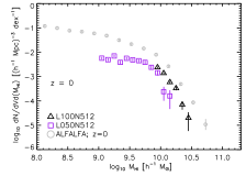
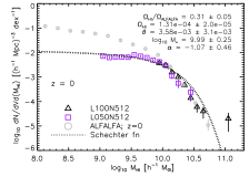
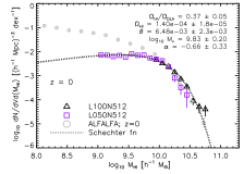
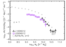
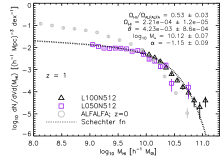
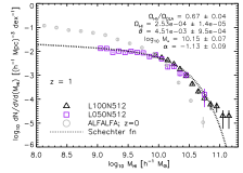
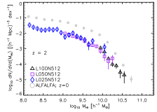
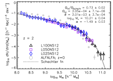
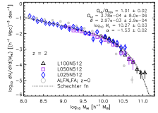
Figure 8: The HI mass function from ZC_WFB at $z=$ 0, 1 and 2; top, middle and bottom respectively, with the $z=0$ ALFALFA HI mass function shown for comparison. Each column displays results for the different self-shielding methods: the left column is method $\rm SS_{None}$ (no self-shielding); the middle column is method $\rm SS_{ALFALFA}$ (pressure threshold tuned to match the ALFALFA data in the range $M_{\rm HI}=10^{10}-10^{11}\,h^{-1}{\rm M_{\odot}}$ ) and the right column is method $\rm SS_{DLA}$ (pressure threshold tuned to match the $z=2$, $\Omega_{\rm DLA}$ results of Prochaska & Wolfe 2009). Typically, the pressure value found to match the $z=2$ DLA results is higher than that used for $z=0$, allowing us to bracket the available range of possible HI mass functions for the ZC_WFB simulations. Poisson errors are assumed for individual simulation data points. We also show a Schechter function fit to the simulated data (for methods $\rm SS_{ALFALFA}$ and $\rm SS_{DLA}$) and present best-fit values for $\alpha$, $\theta$ and $M_{*}$ (and their errors, from bootstrap resampling) in the legend. Values for $\Omega_{\rm HI}$, calculated from the integrated Schechter function, are also shown. Clearly, $\Omega_{\rm HI}\simeq\Omega_{\rm DLA}$ for method $\rm SS_{DLA}$ at $z=2$ but $\Omega_{\rm HI}<\Omega_{\rm ALFALFA}$ in method $\rm SS_{ALFALFA}$ (i.e. this model predicts less HI at high-redshift).

5.1 HI Mass Functions

The HI mass functions for ZC_WFB are shown in Fig. 8. As discussed earlier, we use individual subhaloes to represent the galaxies and we determine the minimum HI mass for each simulation according to the values given in Equation 6. In all cases, the number density of objects decreases as a function of increasing HI mass, with a strongly suppressed high-mass end and a more gradual slope at the faint end (where simulation data is available). The good agreement in abundance at the overlap between the different simulation volumes, increases our confidence in the numerical resolution cuts we have made.

We consider the no-shielding case first (left column of Fig. 8) and can immediately see that at $z=0$, top panel, the simulation points lie below the ALFALFA results. This justifies our assumption that the self-shielding correction (which increases the amount of HI at moderate densities) must be implemented to match observations. In the absence of self-shielding there appears to be little evolution in the HI mass function between $z=0$ and $z=2$.

We can tune the self-shielding pressure threshold to match the ‘knee’ of the $z=0$ ALFALFA mass function and utilise this same pressure cut at higher redshifts, as shown in the middle column of Fig. 8. Interestingly, the simulations predict relatively little change in the abundance of haloes in this mass range with redshift. The high-mass end matches the ALFALFA data very well. At the low-mass end, the simulation under-predicts the number of objects; this flattening is also seen in the cold gas mass function (see Section 5.2) and thus appears to be related to the galaxy formation modelling in the simulation.

The HI mass functions are well parameterised by a Schechter function (particularly at $z=2$ where we have the highest dynamic range) given by

$$\frac{{\rm d}n}{{\rm d}M}=\frac{\theta}{M_{*}}\left(\frac{M}{M_{*}}\right)^{\alpha}{\rm e}^{-\frac{M}{M_{*}}}\,,$$ (7)

with normalisation $\theta$, low-mass slope $\alpha$ and characteristic mass scale $M_{*}$, respectively. This can be integrated to give the mass density

$$\rho = \int^{\infty}_{0}M\,\frac{{\rm d}n}{{\rm d}M}\,{\rm d}M\,,$$ (8)

$$= \theta\int^{\infty}_{0}\left(\frac{M}{M_{*}}\right)^{\alpha+1}{\rm e}^{-\frac{M}{M_{*}}}\,{\rm d}M.$$

The global HI density (assuming the above masses are HI masses) in units of the critical density, $\rho_{\rm crit}$, is then

$$\Omega_{\rm HI}=\theta\Gamma(\alpha+2)M_{*}/\rho_{\rm crit}\,,$$ (9)

where $\Gamma(x)$ is the standard gamma function. Comparing our results at $z=2$ with the low-redshift data, we predict mild evolution of the HI mass function with the global HI density decreasing from $0.7$ to $0.3$ at $z=0$. This has important ramifications for upcoming deep HI surveys such as those to be performed with the Square Kilometre Array which will detect more HI sources than an extrapolation from the $z=0$ mass function would suggest.

Our third method uses a pressure threshold set by matching the integrated mass function of the simulations at $z=2$ to the DLA inferred cosmic density of HI at $z=2.2$ from Prochaska & Wolfe (2009). The right panels in Fig. 8 show that this leads to very similar results as method $\rm SS_{ALFALFA}$. The higher global HI density at $z=2$ leads to a slightly larger value for $M_{*}$ and a slightly steeper low-mass slope, $\alpha$. Again, comparing results with the ALFALFA data, there is only mild evolution in the global HI density with redshift.

For all models there is however strong evolution seen in the low-mass tail, from a steep index of $-1.5$ at $z=2$ to $\geq-1$ at $z=0$. This evolution is also seen in the cold gas mass function in Fig. 10 which indicates that it is not subject to the self-shielding methodology. This result was also seen in semi-analytic work by Power et al. (2010) who found that cold gas was being turned into stars in these low-mass systems.

We summarise the HI evolution in Fig. 9 where we integrate the Schechter function described in Fig. 8 even though we can clearly see in those figures that the low-mass tail undergoes significant evolution in model ZC_WFB and is shallower than measured locally. The high-mass tail appears to show much more gradual evolution over this period. Observers will be constrained to observing only the largest systems so to, crudely, mimc this selection we limit the fit of the Schechter function to HI masses above $10^{10}\,h^{-1}{\rm M_{\odot}}$ and fix the faint end to $-1.5$ (the value we find at $z=2$). In this case we well agree with observations at low redshift and predict little evolution will be measured to high redshift. We show a number of observational measurements in Fig. 9 and, while we did not attempt to make an exhaustive compilation, we consider this a reasonable summary of the current understanding of the cosmic HI density evolution. The results range from direct, local HI detections by Zwaan et al. (2005) and Martin et al. (2010) to a stacking of the HI signal at a moderate redshift by Lah et al. (2007). Then there are inferred cosmic HI densities through the use of HST observations of low-redshift DLA systems traced by MgII absorbers (Rao et al., 2006; Meiring et al., 2011) and then at higher redshift by Prochaska & Wolfe (2009) and Noterdaeme et al. (2009) using SDSS quasar spectra. There is disagreement between these last two results due, primarily, to a more aggressive treatment for the bias affecting strong absorbers in the latter work.

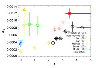
Figure 9: A compilation of some recent measurements of the cosmic HI densities at various epochs. We have included the integrated values for the simulation ZC_WFB (with self-shielding method $\rm SS_{DLA}$) to demonstrate the difficulty in reproducing the observed HI density. Even though at $z=0$ we can reproduce the mass function about the ‘knee’ of the Schechter function, we do not have enough low-mass objects to recover the observed $\Omega_{\rm HI}$. However, if we fix the faint end slope to the value at $z=2$ ($\alpha=-1.5$) and limit the fit to haloes with $M_{\rm HI}>10^{10}\,h^{-1}{\rm M_{\odot}}$ then we recover the blue diamond points which are in better agreement with the low redshift results. They also demonstrate that, in the simulations at least, the evolution in HI is constrained to the faint end. Note that we have tuned the $z=2$ case to agree with Prochaska & Wolfe (2009) rather than the results of Noterdaeme et al. (2009), see text. In our models the evolution of $\Omega_{\rm HI}$ is driven by the low-mass tail, whereas most 21cm observations will be unable to detect this population.

5.2 Molecular and Cold Gas Mass Functions

We now consider the molecular mass function, shown in the left column of Fig. 10, and the more general cold gas mass function, shown in the right column. Cold gas is defined as all gas that is gravitationally bound to the halo and that has temperature $T<10^{4.5}$K, as well as all star-forming gas. Note that neither the cold or molecular gas mass depends on the self-shielding measure used.

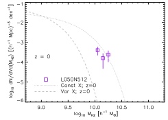
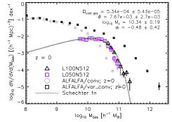
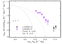
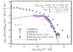
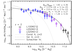
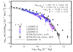
Figure 10: The simulated $\rm H_{2}$ (cold gas) mass function is shown in the left (right) column at $z=$ 0 (top), 1 (middle) and 2 (bottom), with the $z=0$ $\rm H_{2}$ mass function results from the CO mass function of Keres et al. (2003) when using a constant ($X$-factor) conversion or the varying scheme proposed by Obreschkow & Rawlings (2009b) (denoted with the dotted and dashed lines, respectively). The cold gas mass function is estimated by converting the ALFALFA detections through either a constant assumed atomic-molecular ratio or a variable scheme that depends on the disc gas and stellar mass, with both values taken from Power et al. (2010). The errors on the points are Poissonian. We have made a resolution cut in $M_{\rm H2}$ ($M_{\rm Gas}$) using Equation 6. Note that the molecular mass function evolves more strongly than the cold gas mass as the high mass end.

For the $z=0$ molecular hydrogen mass function, top left panel, we have only a limited mass range ($M_{{\rm H}_{2}}\simeq 1-2\times 10^{10}\,h^{-1}{\rm M_{\odot}}$), but the abundance of objects is in reasonably good agreement with the data of Keres et al. (2003), using a constant (X-factor) conversion between CO and H₂ mass. (We implicitly used this conversion rather than the variable measure advocated by Obreschkow & Rawlings 2009b, when we adopted the Leroy et al. 2008 molecular-atomic abundance normalisation.) It is clear that the high-mass end of the Schechter function evolves strongly as a function of redshift, with many more high molecular mass systems at higher redshift. The overall cosmic molecular mass density at $z=2$ is predicted to be a factor two larger than observed locally. Thus, the large increase in stellar density between $z=2$ and the present day is reflected in the molecular mass function rather than the HI mass function, which appears to be demonstrate mild evolution. This overall effect is also seen for a range of other physics schemes probed in Fig. 12.

The cold gas mass function can be estimated observationally by converting the HI mass function from ALFALFA, corrected for the He fraction assuming a molecular - atomic ratio based on the ratio of the global densities of each. As advocated by Power et al. (2010), for a fixed molecular-atomic ratio this conversion is akin to dividing the HI mass by $0.54$. For a conversion factor that depends on galactic scale properties, as considered in Obreschkow & Rawlings (2009b) the HI mass - cold mass conversion factor is given in Equation 4. in Power et al. (2010) as

$$M_{\rm HI}=0.76M_{\rm cold}/(1+R_{\rm surf})\,,$$ (10)

where we previously defined $R_{\rm surf}$ in Equation 4. The exact conversion of HI mass to cold gas mass is especially important at the high-mass end. If we use a variable conversion ratio, then our simulated gas masses are too low at the high-mass end. The situation is reversed in the case of a constant conversion factor. For the case of the constant conversion factor, Power et al. (2010) find that the semi-analytic prescriptions also typically overproduce the number of gas-rich systems. There appears to be a generic disagreement between both hydro and semi-analytic simulations with the data if a constant HI/H₂ is assumed. This lends increasing support to the idea that the ratio depends on the global properties of the system in which it is measured, e.g. as considered in Obreschkow & Rawlings (2009b).

6 Effects of feedback and metal cooling on HI mass function

As we have demonstrated in previous work (Duffy et al., 2010), the gas distribution in a halo can vary significantly with the physics implementation. This is especially true as the ZC_WFB model is unable to remove gas from the largest galaxies, and hence is unable to form red ellipticals by suppressing star formation in the most massive systems. We attempt to analyse the sensitivity of our results to the wide array of possible feedback types, as well as cooling schemes, used in this previous work. We have created the HI mass function at $z=0$ and $2$ for the different physics prescriptions and present these in Fig. 11, again applying the HI mass cut from Equation 6 and tuning each physics simulation independently in the same manner as Section 3.1 with pressure values given in Table 3. Equivalent plots to Fig. 10, for the H₂ and cold gas mass functions, are shown in Fig. 12.

$\rm SS_{None}$	$\rm SS_{ALFALFA}$	$\rm SS_{DLA}$

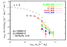
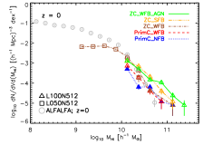
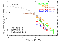
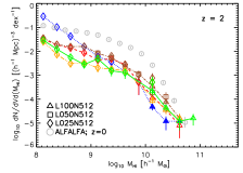
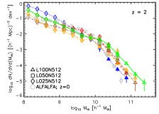
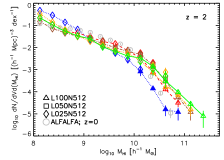
Figure 11: As Fig. 8 but now showing a comparison of HI mass functions for runs with different physics prescriptions, at $z=0$ (top panels) and $z=2$ (bottom panels). Again, the columns show results for self-shielding methods $\rm SS_{None}$, $\rm SS_{ALFALFA}$, $\rm SS_{DLA}$, left to right respectively. The low-redshift result from ALFALFA is also shown for comparison. Note that certain simulations, e.g. PrimC_WFB and PrimC_NFB, have too little cold gas at low redshift that even when setting the $P_{\rm shield}=0$, converting all cold gas in the galaxy to be neutral. This is seen most clearly in the top-middle panel in which the red dashed and blue dotted lines lie below the other simulations at all mass bins.

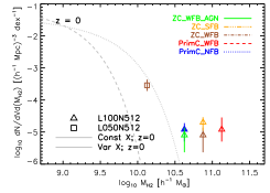
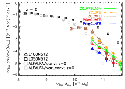
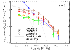
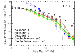
Figure 12: As Fig. 11 but now showing a comparison of H₂ (left) and cold gas (right) mass functions for the different physics prescriptions. The self-shielding method is irrelevant for these results. The grey curves are the $z=0$ $\rm H_{2}$ mass function results from the CO mass function of Keres et al. (2003) when using a constant ($X$-factor) conversion or the varying scheme proposed by Obreschkow & Rawlings (2009b) (denoted with the dotted and dashed lines, respectively).

Without any self-shielding implemented at $z=0$ (top-left panel of Fig. 11) the simulations with strong feedback (ZC_WFB_AGN and ZC_SFB) result in a greater number of massive HI systems than the schemes without effective feedback. This is a result of more cold gas being prevented from forming stars, as seen in the top right panel of Fig. 12. When we tune the self-shielding prescription to match the ALFALFA HI cosmic density (over the HI mass range $10^{10}-10^{11}\,h^{-1}{\rm M_{\odot}}$; method $\rm SS_{ALFALFA}$) the difference between the various physics schemes at $z=0$, top middle panel, is reduced as expected.

At $z=2$ we can tune to the DLA result (method $\rm SS_{DLA}$), shown in the bottom right panel, which also shows very little difference between the schemes, although the run with no feedback (PrimC_NFB) shows a lack of massive HI systems in comparison to the other runs. We see from the molecular and cold gas mass functions at $z=2$ (bottom panels of Fig. 12) that more molecular hydrogen is present at high-redshift, due to both the lack of feedback and time to use up the gas and form stars.

It appears that the HI mass function is at least as sensitive, if not more so, to the modelling of self-shielding as to the sub-grid baryonic physics. This could be seen as an unexpected result and highlights the need for a more careful modelling of the optically thick gas in and around galaxies.

There is significantly more variation in the molecular hydrogen mass function when the baryonic physics is varied, as shown in the left column of Fig. 12. The situation at $z=2$, bottom left panel, is complex but apparently the strong feedback schemes remove large amounts of the densest gas relative to the simulations without feedback. The cold gas at $M_{\rm Gas}\geq 10^{9.5}\,h^{-1}{\rm M_{\odot}}$ is, on the other hand, completely insensitive to the sub-grid physics scheme used provided there is some feedback to suppress the rapid overcooling demonstrated by the PrimC_NFB model in the bottom right panel. The potential paradox presented here between the greater sensitivity of the H₂ to the feedback schemes than the HI when the cold gas also appears insensitive is a consequence of the cold gas having no dependancy on the self-shielding prescription used to calculate the HI. As a result the HI fraction of the cold gas can vary to match the observations, giving a greater freedom in the HI results compared to the H₂ which have no such variability. Thus the cold gas mass across simulations is similar but the distribution of this gas as a function of pressure is not, which is then most easily visible in the H₂ mass functions shown in Fig. 12.

7 Conclusions

We have used hydrodynamical simulations from the OWLS project to investigate the distribution of neutral (atomic HI and molecular H₂) hydrogen in cosmological volumes across the redshift range $z=0-2$. The large suite of simulations allowed us to probe both the effects of numerical resolution and the sub-grid baryonic physics implemented (especially the effects of metal enrichment on the gas cooling rate and the different methods and sources of feedback). In addition, we considered several methods to correct for the lack of self-shielding in our simulations in moderate-high-density regions, where the assumption that the gas is optically thin to a uniform UV/X-ray background breaks down. With this in mind, we have found that, together with an empirical pressure-based law to discern the molecular fraction in galaxies, the distribution of HI can be successfully simulated in our cosmological volumes. We have succeeded in recreating the observed local HI mass function for objects with HI mass greater than $10^{10}\,h^{-1}{\rm M_{\odot}}$ but with a significantly shallower faint-end slope. We consider evolution across the redshift range $z=0-2$ and detect significant increases in low-mass HI objects which corresponds into a small, yet systematic, increase in the HI cosmic density with increasing redshift. If we mimc an observational magnitude limited survey, namely objects with HI masses above $10^{10}\,h^{-1}{\rm M_{\odot}}$, and fix the faint end slope to the $z=2$ value then we find that the inferred cosmic HI density is in better agreement with observations at $z=0$ and that observers will infer little evolution in the period $z=0-2$. During this time the molecular hydrogen component evolves strongly, with many more massive systems in the distant past than now, in qualitative agreement with Obreschkow & Rawlings (2009a).

When comparing the predictions of the simulations with varying physics prescriptions, including an AGN feedback model, we found that the HI mass functions were insensitive to these treatments. Provided one can tune the pressure based self-shielding threshold, we can recover the overall HI distribution to within a factor of two using just a single threshold value.

However, the implementation of the self-shielding threshold has at least as large an effect on the HI mass function than the differences between the sub-grid cooling and feedback models we consider here, these models essentially bracket the extrema of sub-grid implementations and hence to improve on this level of accuracy in the future we will utilise radiative transfer schemes such as in Altay et al. (2010) and Pawlik & Schaye (2008).

For the case of the simulation with supernovae feedback and realistic cooling we found a peak HI - halo mass fraction at a given halo mass across our redshift range, $z=0-2$, which we attribute to two effects. The first is that in more massive haloes the neutral component is dominated by denser $\rm H_{2}$ while at lower masses the overall gas fraction of the halo has been reduced due to feedback. This peak is also found to be the ‘knee’ of the HI mass function, which is well reproduced in our simulation with supernova feedback.

The typical sizes, denoted by the half-mass radius, of the HI, H₂ and stars in this work were found to vary as a function of total halo mass and redshift. We found, however that the HII radius increased with the cube root of the halo mass, characteristic of a smoothly distributed isothermal profile. The typical sizes of the HI disk increased with redshift but that the steepness of this relation with halo mass decreased from a linear dependency to approximately a cube root (tracing of the more diffuse, ionised component). The stars and molecular hydrogen closely traced each other throughout redshift, with an identical half mass radius at galaxy scales, i.e. the pivot mass of $2\times 10^{12}\,h^{-1}{\rm M_{\odot}}$, but differed significantly at $z=0$ for galaxy group and cluster-sizes, with the stellar radius a factor 5 more extended the molecular component. We also tested the feedback from an AGN and found that the molecular and stellar components were more extended than their counterparts in the simulation without an AGN, at all redshifts. This is in agreement with Sales et al. (2010) who studied galaxies at $z=2$ and found that such strong feedback resulted in the formation of large, extended galaxies.

Finally, we have found that the ratio of HI (H₂) to stellar mass of our objects is negatively (positively) correlated with the stellar mass. The normalisation of the model with SNe feedback was found to be in particularly good agreement with observations. Furthermore, we predict that the ratio of HI (H₂) to stellar mass at a given stellar mass increases significantly with redshift. This means that the hydrogen signal from small systems will be easier to find than an extrapolation of from larger optical counterparts would suggest. This improves the chances that optically faint galaxies may be detectable in upcoming ultra-deep 21 cm and molecular hydrogen observations.

Appendix A Resolution Tests

Here we investigate how numerical resolution and simulation box size affect our main results. In particular, we study how increasing the number of particles (and decreasing the gravitational softening length) affects the properties of the same sample of haloes. We also investigate the effects of increasing the simulation volume while keeping the resolution constant. As a result, we identify a simple scaling between the minimum required halo mass (that depends on the particular baryonic species under consideration) and the particle mass. We also show that our results cannot be significantly affected by the lack of structure on scales larger than our available box sizes. Although we consider the case of the neutral phases of hydrogen, similar tests have been performed for the stars and ionised hydrogen to create the mass limits quoted in Equation 6.

A.1 HI mass range

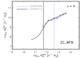
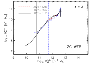
Figure 13: Resolution tests for the HI mass in the FoF group as a function of ${M^{\rm Halo}_{\rm vir}}$ in ZC_WFB. The top panel shows results for the $50\,h^{-1}\,{\rm Mpc}$ box at $z=0$, while the bottom panel is for the 25 $\,h^{-1}{\rm Mpc}$ box at $z=2$. At $z=2\,(0)$ we show results for 3 (2) simulations of the same box, spanning a factor of 64 (8) in particle number/mass. The vertical lines indicate the mass limit given in Equation 6 (roughly speaking this is equivalent to 7,000 dark matter particles) for each run. The curves correspond to haloes an order of magnitude in mass below this limit; the results appear converged, therefore we can be confident with our conservative limit in Equation 6. We bin the haloes that have masses greater than the vertical mass limits and denote their median values with symbols (triangles for the solid curve, squares for the dotted). Errors are $1\sigma$ values, estimated by bootstrap analysis and added in quadrature with Poissonian error estimates.

In order to determine the minimum halo size, and the corresponding HI mass resolution, we select FoF groups from the ‘ZC_WFB’ simulation according to their total mass, $M^{\rm Halo}_{\rm vir}$. After grouping the objects in fixed mass bins we calculate the median HI mass of the bin. The variation in median HI mass with halo mass is shown for two simulation sets in Fig. 13; with increasing resolution in the $50\,h^{-1}{\rm Mpc}$ box at $z=0$ (top panel); and those with increasing resolution in the $25\,h^{-1}{\rm Mpc}$ box at $z=2$ (bottom panel).

As one would expect, the curves demonstrate a positive correlation between HI and halo mass. Those haloes which lie on the same relation between simulations typically have at least $\sim 7,000$ dark matter particles. We adopt a conservative mass limit, shown as a vertical line for each simulation, and identify the HI mass corresponding to this halo mass for each simulation. As mentioned in Section 4.1, we found that we could summarise this limit for all species as a simple power-law scaling relation of the simulation mass resolution, as given in Equation. 6 in the main body of the text. In our study, we have applied this limit to the baryonic masses, resulting in an even more conservative lower HI mass limit.

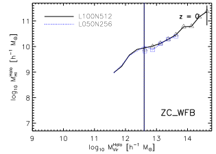
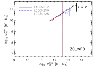
Figure 14: As Fig. 13 but comparing different box sizes (25, 50 & 100 $\,h^{-1}{\rm Mpc}$, where available) at fixed resolution (where available) at $z=0$ and 2.

We also compare the same relation for different simulation volumes at the same resolution in Fig. 14. These demonstrate that the results are insensitive to the total volume simulated.

A.2 HI mass function

Given our established lower HI mass limits, we now investigate the range of masses over which we can trust the HI mass function. To that end we show the HI mass functions for the simulations (going down an order of magnitude in mass) in Fig. 15, illustrating our minimum HI mass cut-off as a vertical line. For comparison we also overplot the datapoints from P09; the resolution of their simulation (with $256^{3}$ dark matter particles in a $32\,h^{-1}{\rm Mpc}$ box) lies in between our $100\,h^{-1}{\rm Mpc}$ and $50\,h^{-1}{\rm Mpc}$ simulations with $512^{3}$ dark matter particles.

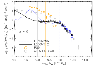
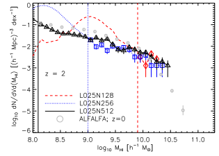
Figure 15: Effects of resolution on the HI mass function for the 50 $\,h^{-1}{\rm Mpc}$ boxes at $z=0$ and the 25 $\,h^{-1}{\rm Mpc}$ boxes at $z=2$ (top and bottom rows respectively). These results span a factor of 64 in particle mass between the lowest and highest resolutions. Lower HI mass limits are shown as vertical lines, above which the abundance of haloes is reasonably well converged (Poisson errors in abundance are assumed). The mass function starts to rises more steeply below the resolution limit, suggesting a numerical artefact. We have also included the $z=0$ data-points from Popping et al. (2009) in the top panel. We note that our HI mass limit applied to their simulation (orange line) suggests that their results may suffer from numerical effects.

It is clear that our mass function is reasonably well converged above our HI mass limits; below these limits there is an artificial rise in the number of haloes, an effect that may be present in the results of P09 (also shown in the figure) who study the mass function down to $3.5\times 10^{8}\,h^{-1}{\rm M_{\odot}}$; we would estimate their resolution limit to be cut at masses 40% higher, close to where their simulations exhibit the characteristic rapid rise in the HI mass function. We have also checked the effects of increasing volume at fixed resolution and find excellent convergence between the simulations.

A.3 Molecular Hydrogen

The molecular hydrogen in the simulations comes from higher density regions in galaxies than the HI and therefore may be expected to be a more demanding quantity to resolve. Again, by comparing the molecular mass from simulations with different resolution but of the same volume, we can determine a resolution-dependent mass limit. As expected, our H₂ mass limit is somewhat higher (by around an order of magnitude) than the HI mass limit, as given in Equation 6.

In Fig. 16 we show the molecular H₂ mass functions for simulations with increasing resolution, in the $50\,h^{-1}{\rm Mpc}$ box at $z=0$ (top panel) and the $25\,h^{-1}{\rm Mpc}$ box at $z=2$ (bottom panel). Vertical lines denote the resolution limits for the simulations. The overlapping curves demonstrate a reasonably well converged result, although it is clear that the mass resolution is extremely demanding. The $z=0$ results from P09 are also shown (we estimate their limit is $5\times 10^{9}\,h^{-1}{\rm M_{\odot}}$, they choose a limit 75 times less than this).

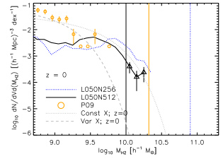
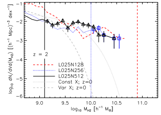
Figure 16: Molecular $\rm H_{2}$ mass functions for simulations with different resolution. The top panel is for the $50\,h^{-1}{\rm Mpc}$ simulation box at $z=0$ and the bottom panel is for the smaller $25\,h^{-1}{\rm Mpc}$ box at $z=2$. Resolution limits are shown as vertical lines and we assume a Poisson error for each data-point. We have also included the $z=0$ data-points from Popping et al. (2009) in the top panel. As in Fig. 15, our resolution limit applied to their simulation (orange line) suggests that their results may suffer from numerical effects. The grey curves are the $z=0$ $\rm H_{2}$ mass function results from the CO mass function of Keres et al. (2003) when using a constant ($X$-factor) conversion or the varying scheme proposed by Obreschkow & Rawlings (2009b) (denoted with the dotted and dashed lines, respectively).

Finally, we have also tested the sensitivity of the molecular mass function to the effects of large-scale structure by reducing the simulation volume at constant mass resolution. As with the HI case, there appears to be excellent agreement between the overlapping box sizes.

References

- Abdalla & Rawlings (2005) Abdalla F. B., Rawlings S., 2005, MNRAS, 360, 27
- Altay et al. (2010) Altay G., Theuns T., Schaye J., Crighton N. H. M., Dalla Vecchia C., 2011, ApJ, 737, L37
- Bandara et al. (2009) Bandara K., Crampton D., Simard L., 2009, ApJ, 704, 1135
- Barnes et al. (2001) Barnes D. G., Staveley-Smith L., de Blok W. J. G., Oosterloo T., Stewart I. M., et al., 2001, MNRAS, 322, 486
- Bate & Burkert (1997) Bate M. R., Burkert A., 1997, MNRAS, 288, 1060
- Booth & Schaye (2009) Booth C. M., Schaye J., 2009, MNRAS, 398, 53
- Booth & Schaye (2010) Booth C. M., Schaye J., 2010, MNRAS, 405, L1
- Chabrier (2003) Chabrier G., 2003, PASP, 115, 763
- Chang et al. (2010) Chang T., Pen U., Bandura K., Peterson J. B., 2010, Nature, 466, 463
- Cole & Lacey (1996) Cole S., Lacey C., 1996, MNRAS, 281, 716
- Crain et al. (2007) Crain R. A., Eke V. R., Frenk C. S., et al., 2007, MNRAS, 377, 41
- Dalla Vecchia & Schaye (2008) Dalla Vecchia C., Schaye J., 2008, MNRAS, 387, 1431
- Davis et al. (1985) Davis M., Efstathiou G., Frenk C. S., White S. D. M., 1985, ApJ, 292, 371
- Dolag et al. (2009) Dolag K., Borgani S., Murante G., Springel V., 2009, MNRAS, 399, 497
- Drory et al. (2003) Drory N., Bender R., Feulner G., Hopp U., Maraston C., Snigula J., Hill G. J., 2003, ApJ, 595, 698
- Drory et al. (2005) Drory N., Salvato M., Gabasch A., Bender R., Hopp U., Feulner G., Pannella M., 2005, ApJL, 619, L131
- Duffy et al. (2008) Duffy A. R., Battye R. A., Davies R. D., Moss A., Wilkinson P. N., 2008, MNRAS, 383, 150
- Duffy et al. (2011) Duffy A. R., Moss A., Staveley-Smith L., 2011, ArXiv e-prints
- Duffy et al. (2010) Duffy A. R., Schaye J., Kay S. T., Dalla Vecchia C., Battye R. A., Booth C. M., 2010, MNRAS, 405, 2161
- Erb et al. (2006) Erb D. K., Shapley A. E., Pettini M., Steidel C. C., Reddy N. A., Adelberger K. L., 2006, ApJ, 644, 813
- Fabello et al. (2011) Fabello S., Catinella B., Giovanelli R., Kauffmann G., Haynes M. P., Heckman T. M., Schiminovich D., 2011, MNRAS, 411, 993
- Ferland et al. (1998) Ferland G. J., Korista K. T., Verner D. A., Ferguson J. W., Kingdon J. B., Verner E. M., 1998, PASP, 110, 761
- Fontana et al. (2004) Fontana A., Pozzetti L., Donnarumma I., Renzini A., Cimatti A., et al., 2004, A&A, 424, 23
- Giovanelli et al. (2005) Giovanelli R., Haynes M. P., Kent B. R., et al., 2005, AJ, 130, 2598
- Haardt & Madau (2001) Haardt F., Madau P., 2001, in Neumann D. M., Tran J. T. V., eds, Clusters of Galaxies and the High Redshift Universe Observed in X-rays Modelling the UV/X-ray cosmic background with CUBA
- Häring & Rix (2004) Häring N., Rix H., 2004, ApJL, 604, L89
- Kennicutt (1998) Kennicutt Jr. R. C., 1998, ARA&A, 36, 189
- Keres et al. (2003) Keres D., Yun M. S., Young J. S., 2003, ApJ, 582, 659
- Komatsu et al. (2011) Komatsu E., Smith K. M., Dunkley J., et al., 2011, ApJS, 192, 18
- Krumholz et al. (2008) Krumholz M. R., McKee C. F., Tumlinson J., 2008, ApJ, 689, 865
- Krumholz et al. (2009) Krumholz M. R., McKee C. F., Tumlinson J., 2009, ApJ, 693, 216
- Lacey & Cole (1994) Lacey C., Cole S., 1994, MNRAS, 271, 676
- Lagos et al. (2011) Lagos C. d. P., Baugh C. M., Lacey C. G., Benson A. J., Kim H.-S., Power C., 2011, ArXiv e-prints
- Lah et al. (2007) Lah P., Chengalur J. N., Briggs F. H., et al., 2007, MNRAS, 376, 1357
- Lang et al. (2003) Lang R. H., Boyce P. J., Kilborn V. A., et al., 2003, MNRAS, 342, 738
- Leroy et al. (2008) Leroy A. K., Walter F., Brinks E., et al., 2008, AJ, 136, 2782
- Madau et al. (1996) Madau P., Ferguson H. C., Dickinson M. E., Giavalisco M., Steidel C. C., Fruchter A., 1996, MNRAS, 283, 1388
- Martin et al. (2010) Martin A. M., Papastergis E., Giovanelli R., Haynes M. P., Springob C. M., Stierwalt S., 2010, ApJ, 723, 1359-1374
- McCarthy et al. (2010) McCarthy I. G., Schaye J., Ponman T. J., Bower R. G., Booth C. M., Vecchia C. D., Crain R. A., Springel V., Theuns T., Wiersma R. P. C., 2010, MNRAS, pp 740–+
- McQuinn et al. (2011) McQuinn M., Oh S. P., Faucher-Giguere C.-A., 2011, ArXiv e-prints
- Meurer et al. (2006) Meurer G. R., Hanish D. J., Ferguson H. C., Knezek P. M., Kilborn V. A., et al., 2006, ApJS, 165, 307
- Meyer et al. (2004) Meyer M. J., Zwaan M. A., Webster R. L., Staveley-Smith L., Ryan-Weber E., et al., 2004, MNRAS, 350, 1195
- Meiring et al. (2011) Meiring, J. D., Tripp, T. M., Prochaska, J. X., Tumlinson, J., Werk, J., Jenkins, E. B., Thom, C., O’Meara, J. M., Sembach, K. R., 2011, ApJ, 732, 35
- Mo et al. (1998) Mo H. J., Mao S., White S. D. M., 1998, MNRAS, 295, 319
- Noterdaeme et al. (2009) Noterdaeme P., Petitjean P., Ledoux C., Srianand R., 2009, A&A, 505, 1087
- Obreschkow et al. (2009) Obreschkow D., Croton D., DeLucia G., Khochfar S., Rawlings S., 2009, ApJ, 698, 1467
- Obreschkow & Rawlings (2009a) Obreschkow D., Rawlings S., 2009a, ApJL, 696, L129
- Obreschkow & Rawlings (2009b) Obreschkow D., Rawlings S., 2009b, MNRAS, 394, 1857
- Pawlik & Schaye (2008) Pawlik A. H., Schaye J., 2008, MNRAS, 389, 651
- Pawlik & Schaye (2009) Pawlik A. H., Schaye J., 2009, MNRAS, 396, L46
- Pontzen et al. (2008) Pontzen A., Governato F., Pettini M., et al., 2008, MNRAS, 390, 1349
- Popping et al. (2009) Popping A., Davé R., Braun R., Oppenheimer B. D., 2009, A&A, 504, 15
- Power et al. (2010) Power C., Baugh C. M., Lacey C. G., 2010, MNRAS, 406, 43
- Pozzetti et al. (2003) Pozzetti L., Cimatti A., Zamorani G., Daddi E., Menci N., et al., 2003, A&A, 402, 837
- Prochaska et al. (2005) Prochaska J. X., Herbert-Fort S., Wolfe A. M., 2005, ApJ, 635, 123
- Prochaska et al. (2010) Prochaska J. X., O’Meara J. M., Worseck G., 2010, ApJ, 718, 392
- Prochaska & Wolfe (2009) Prochaska J. X., Wolfe A. M., 2009, ApJ, 696, 1543
- Quinn et al. (1996) Quinn T., Katz N., Efstathiou G., 1996, MNRAS, 278, L49
- Rao et al. (2006) Rao S. M., Turnshek D. A., Nestor D. B., 2006, ApJ, 636, 610
- Razoumov et al. (2008) Razoumov A. O., Norman M. L., Prochaska J. X., Sommer-Larsen J., Wolfe A. M., Yang Y.-J., 2008, ApJ, 683, 149
- Sales et al. (2010) Sales L. V., Navarro J. F., Schaye J., Dalla Vecchia C., Springel V., Booth C. M., 2010, MNRAS, 409, 1541
- Savaglio et al. (2005) Savaglio S., Glazebrook K., Le Borgne D., Juneau S., Abraham R. G., et al., 2005, ApJ, 635, 260
- Schaye (2001a) Schaye J., 2001a, ApJL, 562, L95
- Schaye (2001b) Schaye J., 2001b, ApJ, 559, 507
- Schaye (2004) Schaye J., 2004, ApJ, 609, 667
- Schaye & Dalla Vecchia (2008) Schaye J., Dalla Vecchia C., 2008, MNRAS, 383, 1210
- Schaye et al. (2010) Schaye J., Dalla Vecchia C., Booth C. M., Wiersma R. P. C., Theuns T., Haas M. R., Bertone S., Duffy A. R., McCarthy I. G., van de Voort F., 2010, MNRAS, 402, 1536
- Seljak & Zaldarriaga (1996) Seljak U., Zaldarriaga M., 1996, ApJ, 469, 437
- Spergel et al. (2007) Spergel D. N., Bean R., Doré O., et al., 2007, ApJS, 170, 377
- Springel (2005) Springel V., 2005, MNRAS, 364, 1105
- Tacconi et al. (2010) Tacconi L. J., Genzel R., Neri R., Cox P., Cooper M. C., et al., 2010, Nature, 463, 781
- Tescari et al. (2009) Tescari E., Viel M., Tornatore L., Borgani S., 2009, MNRAS, 397, 411
- Tremaine et al. (2002) Tremaine S., Gebhardt K., Bender R., Bower G., Dressler A., et al., 2002, ApJ, 574, 740
- Tremonti et al. (2004) Tremonti C. A., Heckman T. M., Kauffmann G., Brinchmann J., Charlot S., et al., 2004, ApJ, 613, 898
- van de Voort et al. (2011a) van de Voort F., Schaye J., Booth C. M., Dalla Vecchia C., 2011, MNRAS, pp 805–+
- van de Voort et al. (2011b) van de Voort F., Schaye J., Booth C. M., Haas M. R., Dalla Vecchia C., 2011, MNRAS, 414, 2458
- Wiersma et al. (2009) Wiersma R. P. C., Schaye J., Smith B. D., 2009, MNRAS, 393, 99
- Wiersma et al. (2009) Wiersma R. P. C., Schaye J., Theuns T., Dalla Vecchia C., Tornatore L., 2009, MNRAS, 399, 574
- Zwaan et al. (2005) Zwaan M. A., Meyer M. J., Staveley-Smith L., Webster R. L., 2005, MNRAS, 359, L30
- Zwaan et al. (2003) Zwaan M. A., Staveley-Smith L., Koribalski B. S., et al., 2003, AJ, 125, 2842