Genericity aspects in gravitational collapse to black holes and naked singularities

Abstract

We investigate here the genericity and stability aspects for naked singularities and black holes that arise as the final states for a complete gravitational collapse of a spherical massive matter cloud. The form of the matter considered is a general Type I matter field, which includes most of the physically reasonable matter fields such as dust, perfect fluids and such other physically interesting forms of matter widely used in gravitation theory. We first study here in some detail the effects of small pressure perturbations in an otherwise pressure-free collapse scenario, and examine how a collapse evolution that was going to the black hole endstate would be modified and go to a naked singularity, once small pressures are introduced in the initial data. This allows us to understand the distribution of black holes and naked singularities in the initial data space. Collapse is examined in terms of the evolutions allowed by Einstein equations, under suitable physical conditions and as evolving from a regular initial data. We then show that both black holes and naked singularities are generic outcomes of a complete collapse, when genericity is defined in a suitable sense in an appropriate space.

I Introduction

The aim of the present work is twofold. Firstly, we study here the effect of introducing small pressure perturbations in an otherwise pressure-free gravitational collapse which was to terminate in a black hole final state. For such a purpose, spherically symmetric models of black hole and naked singularity formation for a general matter field are considered, which undergo a complete gravitational collapse under reasonable physical conditions while satisfying suitable energy conditions. Secondly, we investigate the genericity and stability aspects of the occurrence of naked singularities and black holes as collapse endstates. The analysis of pressure perturbations in known collapse models, inhomogeneous but otherwise pressure-free, shows how collapse final states in terms of black hole or naked singularity are affected and altered. This allows us to examine in general how generic these outcomes are and we study in the initial data space the set of conditions that lead the collapse to a naked singularity and investigate how ‘abundant’ these are. While it is known now for some time that both black holes and naked singularities do arise as collapse endstates under reasonable physical conditions, this helps us understand and analyze in a clear manner the genericity aspects of occurrence of these objects in a complete gravitational collapse of a massive matter cloud in general relativity.

The physics that is accepted today as the backbone of the general mechanism describing the formation of black holes as the endstate of collapse relies on the very simple and widely studied Oppenheimer-Snyder-Datt (OSD) dust model, which describes the collapse of a spherical cloud of homogeneous dust OSD , Datt . In the OSD case, all matter falls into the singularity at the same comoving time while an horizon forms earlier than the singularity, thus covering it. A black hole results as the endstate of collapse. Still, homogeneous dust is a highly idealized and unphysical model of matter. Taking into account inhomogeneities in the initial density profile it is possible to show that the behaviour of the horizon can change drastically, thus leaving two different outcomes as the possible result of generic dust collapse: the black hole, in which the horizon forms at a time anteceding the singularity, and the naked singularity, in which the horizon is delayed thus allowing null geodesics to escape the central singularity where the density and curvatures diverge, to reach faraway observers dust1 -dust5 .

It is known now that naked singularities do arise as a general feature in General Relativity under a wide variety of circumstances. Many examples of singular spacetimes can be found, but their relevance in models describing physically viable scenarios has been a matter of much debate since the first formulation of the Cosmic Censorship Hypothesis (CCH) Penrose . In particular, the formation of naked singularities in dynamical collapse solutions of Einstein field equations remains a much discussed problem of contemporary relativity. The CCH, which states that any singularity occurring in the universe must be hidden within an event horizon and therefore not visible to faraway observers, has remained at the stage of a conjecture for more than four decades now. This is also because of the difficulties lying in a concrete and definitive formulation of the conjecture itself. While no proof or any mathematically rigorous formulation of the same exists in the context of dynamical gravitational collapse (while some proofs exist for particular classes of spacetimes that do not describe gravitational collapse, as in Dafermos1 and Dafermos2 ), many counterexamples have been found over the past couple of decades Ref1 -Ref6 . Many of these collapse scenarios are restricted by some simplifying assumptions such as the absence of pressures (dust models) or the presence of only tangential pressures tang1 -tang7 . It is well-known that the pressures cannot be neglected in realistic models describing stars in equilibrium. It seems natural therefore that if one wishes to study analytically what happens during the last stages of the life of a massive star, when its core collapses under its own gravity thus forming a compact object as a remnant, pressures must be taken into account.

Therefore, further to early works that showed the occurrence of naked singularities in dust collapse, much effort has been devoted to understanding the role played by pressures press1 -press7 . The presence of pressures is a crucial element towards the description of realistic sources as we know that stars and compact objects are generally sustained by matter with strong stresses (either isotropic or anisotropic). At first it was believed that the naked singularity scenario could be removed by the introduction of pressures, thus implying that more realistic matter models would lead only to the formation of a black hole. We now know that this is not the case. The final outcome of collapse with pressure is entirely decided by its initial configuration and allowed dynamical evolutions and it can be either a black hole or a naked singularity. Furthermore it is now clear that within spherical collapse models (be it dust, tangential pressure or others) the data set leading to naked singularities is not a subset of ‘zero measure’ of the set of all possible initial data.

Despite all this work we can still say that much more is to be understood about the role that general pressures play during the final stages of collapse. Perfect fluid collapse has been studied mostly under some simplifying assumptions and restrictions in order to gain an understanding, but a general formalism for perfect fluids described by a physically valid equation of state is still lacking due to the intrinsic difficulties arising from Einstein equations. Considering both radial and tangential pressures is a fundamental step in order to better understand what happens in the ultra-dense regions that forms at the center of the collapsing cloud prior to the formation of the singularity. For this reason, perfect fluids appear as a natural choice since these are the models that are commonly used to describe gravitating stars in equilibrium and since it can be shown that near the center of the cloud regularity implies that matter must behave like a perfect fluid.

In the present paper we use a general formalism to analyze the structure of collapse in the presence of perfect fluid pressures. This helps to understand better realistic collapse scenarios and their outcomes and brings out clearly the role played by pressures towards the formation of black holes or naked singularities as the endstate of collapse. We examine what are the key features that determine the final outcome of collapse in terms of a black hole or a naked singularity when perfect fluids, without any restriction imposed by the choice of an equation of state, are considered. The reason we do not assume an explicit equation of state here is that the behavior of matter in ultra-dense states in the final stages of collapse is unknown. On the other hand, having regularity and energy conditions satisfied provides a physically reasonable framework to study collapse endstates.

We find that not only naked singularities are not ruled out in perfect fluid collapse scenarios but also that the separation between the black hole region and the naked singularity region in the space of all possible evolutions has some interesting features. In particular, we show that the introduction of small pressures can drastically change the final fate of the well-known pressureless models. For example, we see that adding a small pressure perturbation to an inhomogeneous dust model leading to a black hole can be enough to change the outcome of collapse to a naked singularity, and viceversa.

Further to this, we investigate here the space of initial data and collapse evolutions in generality, in order to examine the genericity of naked singularities in collapse. To study small pressure perturbations as well as the genericity and stability aspects, we use the general formalism for spherically symmetric collapse developed earlier ndim1 , ndim2 in order to address the basic problem of how generic is a given collapse scenario which leads to the formation of naked singularities. Given the existence of an increasing number of models describing collapse leading to a naked singularity, the issue of genericity and stability of such models in the space of initial data has become the crucial ingredient in order to decide whether the Cosmic Censorship Hypothesis in its present form should be conserved, modified or dropped altogether.

It should be noted, however, that the concepts such as genericity and stability are far from well-defined in a unique manner in general relativity, as opposed to the Newtonian gravity. A major difficulty towards such a task is the non-uniqueness of topology, or the concept of ‘nearness’ itself in a given spacetime geometry HE . One could define topology on a space of spacetime metrics by requiring that the metric component values are ‘nearby’ or also additionally requiring that their $n$-th derivatives are also nearby, and in each case the resulting topologies will be different. This is in fact connected in a way with the basic problem in arriving at a well-formulated statement of the cosmic censorship itself. There have been attempts in the past to examine the genericity and stability of naked singularities in special cases. For example, in C it was shown that for certain classes of massless scalar field collapse the initial data leading to naked singularity has, in a certain sense, a positive codimension, and so the occurrence of naked singularity is unstable in that sense. On the other hand, it was shown in Sar-Pramana , SG that naked singularity occurrence is stable in the sense of the data sets leading to the same being open in the space of initial data. But these need not be dense in this space and so ‘non-generic’ if we use the definition of ‘genericity’ in the sense given in the dynamical systems theory (where a set of initial data leading to a certain outcome is said to be generic if it is open and dense within the set of all initial data). In that case, however, both black hole and naked singularity final states turn out to be ‘non-generic’.

Therefore, in the following we adopt a more physical definition of ‘genericity’ in the sense of ‘abundance’, and we call generic an initial data set that has a non-zero measure, and which is open (though not necessarily dense) in the set of all initial data. With this definition, the results obtained in Sar-Pramana and SG would mean that both black hole and naked singularity are generic collapse endstates. We note that we do not deal here with the self-similar models, or scalar fields, which is a somewhat special case. Therefore, the issue of genericity and stability of naked singularities in collapse remains wide open, for spherically symmetric as well as non-spherical models and for different forms of matter fields. Our consideration here treats in this respect a wide variety of physically reasonable matter fields for spherically symmetric gravitational collapse.

In section II, the general structure for Einstein equations to study spherical collapse is reviewed and we describe how the equations can be integrated thus obtaining the equation of motion for the system. In Section III we examine the structure of the initial data sets of collapse leading to black hole and naked singularity to gain an insight on genericity of such outcomes for some special models and effect of introducing small pressure perturbations is investigated. Section IV then considers the genericity aspects of the outcomes of collapse with respect to initial data sets. We prove that the initial data sets leading to black holes and naked singularities in the space of all initial data sets for perfect fluid collapse are both generic. Section V is devoted to a brief discussion on equations of state. Finally, in section VI we outline the key features of the above approach and its advantages, and point to possible future uses of the same for astrophysical and numerical applications.

II Dynamical evolution of collapse

In this section we summarize and review the key features on spherical gravitational collapse analysis, and also reformulate some of the key quantities and equations, especially those relating to the nature and behaviour of the final singularity curve. This will be useful in a later section in analyzing the small pressure perturbations in a given collapse scenario, and subsequently towards a general analysis of the genericity aspects of the occurrence of naked singularities and black holes as collapse final states.

The regularity conditions and energy conditions that give physically reasonable models are discussed here. The final stages of collapse are discussed, evaluating key elements that determine when the outcome will be a black hole or a naked singularity. We shall find a function, related to the tangent of outgoing geodesics at the singularity whose sign solely determines the time of formation of trapped surfaces in relation with the time of formation of the singularity. We also analyze here the occurrence of trapped surfaces during collapse and the possibility that radial null geodesics do escape thus making it visible. We see how both features are related to the sign of the above mentioned function, thus obtaining a necessary and sufficient condition for the visibility of the singularity.

II.1 Einstein equations

The most general spacetime describing a spherically symmetric collapsing cloud in comoving coordinates $r$ and $t$ depends upon three functions $\nu(r,t)$, $\psi(r,t)$ and $R(r,t)$, and takes the form,

$$ds^{2}=-e^{2\nu(t,r)}dt^{2}+e^{2\psi(t,r)}dr^{2}+R(t,r)^{2}d\Omega^{2}\;.$$ (II.1)

The energy momentum tensor reads,

$$T_{t}^{t}=-\rho;\;T_{r}^{r}=p_{r};\;T_{\theta}^{\theta}=T_{\phi}^{\phi}=p_{\theta}\;,$$ (II.2)

where $\rho$ is the energy density and $p_{r}$ and $p_{\theta}$ are the radial and tangential stresses. The metric functions $\nu$, $\psi$ and $R$ are related to the energy-momentum tensor via the Einstein equations that can be written in the form:

$$p_{r} = -\frac{\dot{F}}{R^{2}\dot{R}}\;,$$ (II.3)

$$\rho = \frac{F^{\prime}}{R^{2}R^{\prime}}\;,$$ (II.4)

$$\nu^{\prime} = 2\frac{p_{\theta}-p_{r}}{\rho+p_{r}}\frac{R^{\prime}}{R}-\frac{p_{r}^{\prime}}{\rho+p_{r}}\;,$$ (II.5)

$$2\dot{R}^{\prime} = R^{\prime}\frac{\dot{G}}{G}+\dot{R}\frac{H^{\prime}}{H}\;,$$ (II.6)

$$F = R(1-G+H)\;,$$ (II.7)

where $F$ is the Misner-Sharp mass of the system (representing the amount of matter enclosed in the comoving shell labeled by $r$ at the time $t$) and for convenience we have defined the functions $H$ and $G$ as,

$$H=e^{-2\nu(r,v)}\dot{R}^{2},\;G=e^{-2\psi(r,v)}R^{\prime 2}.$$ (II.8)

The collapse scenario is obtained by requiring $\dot{R}<0$ and the central ‘shell-focusing’ singularity is achieved for $R=0$, where the density and spacetime curvatures blow up. Divergence of $\rho$ is obtained also whenever $R^{\prime}=0$, thus indicating the presence of a ‘shell-crossing’ singularity. Such singularities are generally believed to be gravitationally weak and do not correspond to divergence of curvature scalars, therefore indicating that they are removable by a suitable change of coordinates cross1 ,cross2 . For this reason in the forthcoming discussion we will be concerned only with the shell-focusing singularity thus assuming $R^{\prime}>0$.

Since there is a scale invariance degree of freedom we can choose the initial time in such a way so that $R(r,t_{i})=r$. Therefore we can introduce the scaling function $v(r,t)$ defined by,

$$R=rv\;,$$ (II.9)

with $v(r,t_{i})=1$, so that the collapse will be described by $\dot{v}<0$ and the singularity will be reached at $v=0$. We see that this is a better definition for the singularity since at $v\neq 0$ the energy density does not diverge anywhere on the spacelike surfaces, including at the center $r=0$. This is seen immediately from the regular behaviour of the mass function near the center that imposes that $F$ must go like $r^{3}$ close to $r=0$ (as it will be shown later). Such a regularity was not clear from equation (II.4), especially along the central curve $r=0$, where we have $R=0$, without the introduction of $v$. In this manner the divergence of $\rho$ is only reached at the singularity. We note that $v$ acts like a label for successive events near the singularity since it is monotonically decreasing in $t$ and therefore can be used as a ‘time’ coordinate in the place of $t$ itself near the singularity.

We shall consider the Misner-Sharp mass to be in general a function of the comoving radius $r$ and the comoving time $t$, expressed via the ‘temporal’ label $v$ as

$$F=F(r,v(r,t))\;.$$ (II.10)

Near the center of the cloud this is just equivalent to a rewriting $F(r,t)$.

It can be shown that vanishing of the pressure gradients near the center of the cloud imply that the radial and tangential stresses must assume the same value in the limit of approach to the center ndim1 . This requirement comes from the fact that the metric functions should be at least $\mathcal{C}^{2}$ at the center of the cloud and is a consequence of the fact that the Einstein equation (II.5) for a general fluid contains a term in $p_{r}-p_{\theta}$ that therefore must vanish at $r=0$. Since we are interested in the final stages of collapse of the core of a star it is therefore straightforward to take that the cloud behaves like a perfect fluid in proximity of $r=0$. We shall then take,

$$p_{r}=p_{\theta}=p\;.$$

In such a case, we are then left with five equations in the six unknowns $\rho$, $p$, $F$, $\nu$, $\psi$ and $v$. The system becomes closed once an equation of state for the fluid matter is defined or assumed, but in general it is possible to study physically valid dynamics (namely those satisfying regularity and energy conditions) without assuming a priori an equation of state. In fact it is reasonable to suppose that any equation of state that holds at the departure from equilibrium, when the gravitational collapse commences, will not continue to hold in the extreme regimes achieved when approaching the singularity. In this case, we are then left with the freedom to choose one of the functions. If we take $F$ as the free function then from Einstein equations (II.3) and (II.4), $p$ and $\rho$ will follow immediately and they can be evaluated explicitly once we know $v$ and its derivatives.

Further, from the requirement for perfect fluid collapse we can write equation (II.5) as

$$\nu^{\prime}=-\frac{p^{\prime}}{\rho+p}\;.$$ (II.11)

Equation (II.6) can be integrated once we define a suitable function $A(r,v)$ from

$$A_{,v}=\nu^{\prime}\frac{r}{R^{\prime}}\;.$$ (II.12)

Then we get,

$$G(r,v)=b(r)e^{2A(r,v)}\;,$$ (II.13)

where the integration function $b(r)$ can be interpreted in analogy with the dust models and is seen to be related to the velocity of the infalling matter shells.

Finally, from equation (II.7) we can write the equation of motion for $R$ in the form of an effective potential as

$$\dot{R}^{2}=e^{2\nu}\left(\frac{F}{R}+G-1\right)\;.$$ (II.14)

This allows us to study the dynamics of the collapsing system in analogy of the usual phase-space tools of the classical mechanics type models.

Equation (II.14) can be expressed in terms of the scaling factor $v$ as,

$$\dot{v}=-e^{\nu}\sqrt{\frac{F}{r^{3}v}+\frac{be^{2A}-1}{r^{2}}}\;,$$ (II.15)

where the minus sign has been considered in order to study the collapse. We see that in order to have a solution we must have $\left(\frac{F}{r^{3}v}+\frac{be^{2A}-1}{r^{2}}\right)>0$, we can call this a ‘reality condition’ that is necessary for the collapse dynamics to occur. Solving the equation (II.15) solves the set of Einstein equations.

II.2 Regularity and energy conditions

Einstein equations provide the relations between the spacetime geometry and the matter distribution within it, however, they do not give any statement about the type of matter that is responsible for the geometry. On a physical ground, not every type of matter distribution is allowed, and therefore some restrictions on the possible matter models must be made based on considerations of physical reasonableness. This usually comes in the form of energy conditions ensuring the positivity of mass-energy density.

Further, regularity conditions must be imposed in order for the matter fields to be well-behaved at the initial epoch from which the collapse evolves and at the center of the cloud. Firstly, the finiteness of the energy density at all times anteceding the singularity and regularity of the Misner-Sharp mass in $r=0$ imply that in general we must have,

$$F(r,t)=r^{3}M(r,v(r,t))\;,$$ (II.16)

where $M$ is a regular function going to a finite value $M_{0}$ in the limit of approach to the center. If $F$ does not go as $r^{3}$ or higher power in the limit of approach to the center $r=0$, we immediately see from the Einstein equation for $\rho$ that there would be a singularity at the center at the initial epoch, which is not allowed by the regularity conditions as we are interested in collapse from regular initial configurations. Also, requiring that the energy density has no cusps at the center is reflected in the condition,

$$M^{\prime}(0,v)=0\;.$$ (II.17)

As seen before, the behaviour of the pressure gradients near $r=0$ suggests that the tangential and radial pressures become equal in limit of approach to the center, thus justifying our assumption of a perfect fluid type of matter. Further since the gradient of the pressures must vanish at $r=0$, we see that $p^{\prime}\simeq r$ near $r=0$ which for the metric function $\nu$ implies that near the center,

$$\nu(r,t)=r^{2}g(r,v(r,t))+g_{0}(t)\;,$$ (II.18)

where the function $g_{0}(t)$ can be absorbed in a redefinition of the time coordinate $t$. From the above, via equation (II.12) we can write

$$A_{,v}=\frac{2g+rg^{\prime}}{R^{\prime}}r^{2}\;.$$ (II.19)

From the analogy with the Lemaitre-Tolman-Bondi (LTB) models we can evaluate the regularity requirements for the velocity profile $b(r)$. Since near the center $b$ can be written as,

$$b(r)=1+r^{2}b_{0}(r)\;,$$ (II.20)

we now see how to interpret the free function $b(r)$ in relation with the known LTB dust models. In fact the cases with $b_{0}$ constant are equivalent to the bound ($b_{0}<0$), unbound ($b_{0}>0$) and marginally bound ($b_{0}=0$) LTB collapse models. Also, the condition that there be no shell-crossing singularities may imply some further restrictions on $b$.

As is known, matter models describing physically realistic sources must be constrained by some energy conditions. The weak energy condition in our case implies

$$\rho\geq 0,\;\rho+p\geq 0\;.$$ (II.21)

The first one is achieved whenever $F^{\prime}>0$. In fact from equation (II.4) we see that positivity of $\rho$ is compatible with positivity of $R^{\prime}$ only if $F^{\prime}>0$. Therefore we must have

$$3M+rM^{\prime}\geq 0\;,$$ (II.22)

that close to the center will be satisfied whenever $M(0,v)\geq 0$. Now from $M^{\prime}=M_{,r}+M_{,v}v^{\prime}$ we can rewrite $\rho$ as

$$\rho=\frac{3M+rM_{,r}-M_{,v}v}{v^{2}R^{\prime}}-p\;,$$ (II.23)

from which we see that the second weak energy condition is satisfied whenever

$$3M+rM_{,r}-M_{,v}v\geq 0\;.$$ (II.24)

Finally the choice of a mass profile satisfying the above equation allows us to rewrite the condition (II.22) as

$$3M+rM_{,r}-M_{,v}v\geq-M_{,v}R^{\prime}\;,$$ (II.25)

which is obviously satisfied if the pressure is positive (since it implies $M_{,v}<0$) but can be satisfied also by some choice of negative pressure profiles.

The dynamical evolution of collapse is entirely determined once the initial data set is given Initial1 -Initial4 . Specifying the initial conditions consists in prescribing the values of the three metric functions and of the density and pressure profiles as functions of $r$ on the initial time surface given by $t=t_{i}$. This reduces to defining the following functions:

$$\rho(r,t_{i})=\rho_{i}(r),\;p(r,t_{i})=p_{i}(r),\;R(r,t_{i})=R_{i}(r),\;\nu(r,v(r,t_{i}))=\nu_{i}(r),\;\psi(r,t_{i})=\psi_{i}(r).$$

At the initial time the choice of the scale function $v$ is such that $R_{i}=r$, furthermore, from $R^{\prime}_{i}=1$ we get $v^{\prime}(r,t_{i})=0$.

Since the initial data must obey Einstein equations it follows that not all of the initial value functions can be chosen arbitrarily. In fact the choice of the mass profile together with Einstein equations is enough to specify the four remaining functions. From equations (II.4) and (II.16), writing

$$M_{i}(r)=M(r,v(r,t_{i}))=M(r,1)\;,$$ (II.26)

we get

$$\rho_{i}=3M_{i}(r)+rM_{i}^{\prime}(r)\;,$$ (II.27)

while from equation (II.3) we get,

$$p_{i}=-(M_{,v})_{i}\;.$$ (II.28)

From equation (II.5) we can write,

$$\nu_{i}(r)=r^{2}g(r,v(r,t_{i}))=r^{2}g_{i}(r)\;.$$ (II.29)

with $g_{i}(r)$ related to $M_{i}$ by

$$2rg_{i}+r^{2}g^{\prime}_{i}=-\frac{p_{i}^{\prime}}{\rho_{i}+p_{i}}\;.$$ (II.30)

In turn, $\nu_{i}$ can be related to the function $A$, defined by equation (II.12), at the initial time via equation (II.19),

$$A_{,v}(r,v(r,t_{i}))=(A_{,v})_{i}=2g_{i}r^{2}+g_{i}^{\prime}r^{3}\;.$$ (II.31)

Finally, the initial condition for $\psi$ can be related to the initial value of the function $A(r,t)$ from equation (II.6) and equation (II.12),

$$A(r,v(r,t_{i}))=A_{i}(r)=-\psi_{i}-\frac{1}{2}\ln b(r)\;.$$ (II.32)

Since we are studying the final stages of collapse and the formation of black holes and naked singularities, we must require the initial configuration to be not trapped. This will allow for the formation of trapped surfaces during collapse and therefore we must require

$$\frac{F_{i}(r)}{R_{i}}=r^{2}M_{i}(r)<1\;,$$ (II.33)

from which we see how the choice of the initial matter configuration $M_{i}$ is related to the initial boundary of the collapsing cloud. Some restrictions on the choices of the radial boundary must be made in order not to have trapped surfaces at the initial time. This condition is reflected on the initial configuration for $G$ and $H$ since $1-\frac{F}{R}=G-H$ and this condition also gives some constraints on the initial velocity. In fact to avoid trapped surfaces at the initial time the velocity of the infalling shells must satisfy

$$|\dot{R}|>\sqrt{b}e^{A+\nu}\;.$$ (II.34)

We see that the initial velocity of the cloud must always be positive and that the case of equilibrium configuration where $\dot{R}=0$ can be taken only in the limit.

The consideration of a perfect fluid matter model implies that the Misner-Sharp mass is in general not conserved during collapse. Therefore the matching with an exterior spherically symmetric solution leads to consider the generalized Vaidya spacetime. It can be proven that matching to a generalized Vaidya exterior is always possible when the collapsing cloud is taken to have compact support within the boundary taken at $r=r_{b}$, and the pressure of the matter is assumed to vanish at the boundary matching1 -matching4 . Matching conditions imply continuity of the metric and its first derivatives across the boundary surface. Such a matching is in principle always possible but it should be noted that matching conditions together with regularity and energy conditions, might impose some further restrictions on the allowed initial configurations.

In the following we are interested in the local visibility of the central singularity occurring at the end of the collapse. Therefore we will restrict our attention to a neighborhood of the central line $r=0$. In this case it is easy to see that there always exist a neighborhood for which no shell crossing singularities occur. This is seen by the fact that $R^{\prime}=v+rv^{\prime}$ and therefore, since $v>0$ and shell crossing singularities are defined by $R^{\prime}=0$, we can always fulfill $R^{\prime}>0$ in the vicinity of the center. Furthermore, as it was mentioned before, matter behaves like a perfect fluid close to the center. This can be seen from the fact that regularity of the metric functions at the initial time requires that $\nu^{\prime}$ does not blow up at the regular center. This in turn implies that from equation (II.5) we must have $p_{r}(0,t_{i})-p_{\theta}(0,t_{i})=0$, and the condition holds for any time $t$ before the singularity.

II.3 Collapse final states

We study now the possible outcomes of collapse evolution. It is known that in general the final fate of the complete collapse of the matter cloud will be either a black hole or a naked singularity, depending on the choice of the initial data and the dynamical evolutions as allowed by the Einstein equations.

In order to analyze the final outcome of collapse we shall perform a change of coordinates from $(r,t)$ to $(r,v)$, thus considering $t=t(r,v)$. As mentioned earlier this is always possible near the center of the cloud due to the monotonic behaviour of $v$. In this case the derivative of $v$ with respect to $r$ in the $(r,t)$ coordinates shall be considered as a function of the new coordinates, $v^{\prime}=w(r,v)$. We see that regularity at the center of the cloud implies $w\rightarrow 0$ as $r\rightarrow 0$.

We can then consider the metric function $\nu=\nu(r,v)$ which is given by equation (II.5), which now becomes,

$$\nu^{\prime}=\frac{M_{,vr}v+(M_{,vv}v-2M_{,v})w}{(3M+rM_{,r}-M_{,v}v)v}R^{\prime}\;,$$ (II.35)

where now $R^{\prime}=v+rw$ and _,r denotes derivative with respect to $r$ in the $(r,v)$ coordinates. This implies,

$$A(r,v)=\int_{v}^{1}\frac{M_{,vr}v+(M_{,vv}v-2M_{,v})w}{(3M+rM_{,r}-M_{,v}v)v}rdv\;.$$ (II.36)

For the sake of clarity, we may assume here that near the center the mass function $M(r,v)$ can be written as a series as,

$$M(r,v)=M_{0}(v)+M_{1}(v)r+M_{2}(v)r^{2}+o(r^{4})\;.$$ (II.37)

As a regularity condition, we take $M_{1}=0$ and $A\simeq r^{2}$. The function $A$ can then be written as an expansion and it takes the form,

$$A(r,v)=A_{2}(v)r^{2}+A_{3}(v)r^{3}+o(r^{4})\;,$$ (II.38)

with the first terms $A_{i}(v)$ given by

$$A_{2} = \int_{v}^{1}\frac{2M_{2,v}+\left(M_{0,vv}-\frac{2M_{0,v}}{v}\right)w_{,r}}{3M_{0}-M_{0,v}v}dv\;,$$ (II.39)

$$A_{3} = \frac{1}{2}\int_{v}^{1}\frac{6M_{3,v}+\left(M_{0,vv}-\frac{2M_{0,v}}{v}\right)w_{,rr}}{3M_{0}-M_{0,v}v}dv\;.$$ (II.40)

If we restrict our analysis to constant $v$ surfaces then in equation (II.40) we can put $w$ and its derivatives to be zero. On the other hand if we approach the singularity along a generic curve we cannot neglect the terms in $w$.

The equation of motion (II.15) takes the form

$$\dot{v}=-e^{\nu}\sqrt{\frac{M}{v}+\frac{be^{2A}-1}{r^{2}}}\;,$$ (II.41)

which can be inverted to give the function $t(r,v)$ that represents the time at which the comoving shell labeled $r$ reaches the event $v$,

$$t(r,v)=t_{i}+\int_{v}^{1}\frac{e^{-\nu}}{\sqrt{\frac{M}{v}+\frac{be^{2A}-1}{r^{2}}}}dv\;.$$ (II.42)

Then the time at which the shell labeled by $r$ becomes singular can be written as a singularity curve as

$$t_{s}(r)=t(r,0)=t_{i}+\int_{0}^{1}\frac{e^{-\nu}}{\sqrt{\frac{M}{v}+\frac{be^{2A}-1}{r^{2}}}}dv\;.$$ (II.43)

Regularity ensures that, in general, $t(r,v)$ is at least $\mathcal{C}^{2}$ near the singularity and therefore can be expanded as,

$$t(r,v)=t(0,v)+\chi_{1}(v)r+\chi_{2}(v)r^{2}+o(r^{3})\;,$$ (II.44)

with

$$t(0,v)=t_{i}+\int_{v}^{1}\frac{1}{\sqrt{\frac{M_{0}}{v}+b_{0}(0)+2A_{2}}}dv\;,$$ (II.45)

and $\chi_{1}=\frac{dt}{dr}\rvert_{r=0}$ and $\chi_{2}=\frac{1}{2}\frac{d^{2}t}{dr^{2}}\rvert_{r=0}$.

Of course the situations with discontinuities can be analyzed as well with minor technical modifications to the above formalism. In our case, assuming that $t(r,v)$ can be expanded implies that the first two terms in the expansion of $A(r,v)$ must vanish. As seen before vanishing of first term is consistent with the regularity condition for $\nu$ that follows from the pressure gradients at the center, while vanishing of second term implies that $M_{1}$ must be a constant, which gives, in accordance with the requirement that the energy density has no cusps at the center, that $M_{1}=0$. The singularity curve then takes the form

$$t_{s}(r)=t_{0}+r\chi_{1}(0)+r^{2}\chi_{2}(0)+o(r^{3})\;,$$ (II.46)

where $t_{0}=t(0,0)$ is the time at which the central shell becomes singular.

By a simple calculation, retaining for the sake of completeness all the terms in the expansions of $M$ and expanding $\nu$ as $\nu=g_{2}(v)r^{2}+...$, we obtain

$$\chi_{1}(v)=-\frac{1}{2}\int_{v}^{1}\frac{\frac{M_{1}}{v}+b_{01}+2A_{3}}{\left(\frac{M_{0}}{v}+b_{00}+2A_{2}\right)^{\frac{3}{2}}}dv\;,$$ (II.47)

and

$$\chi_{2}(v)=\int_{v}^{1}\left[\frac{3}{8}\frac{(\frac{M_{1}}{v}+b_{01}+2A_{3})^{2}}{\left(\frac{M_{0}}{v}+b_{00}+2A_{2}\right)^{\frac{5}{2}}}-\frac{g_{2}}{\sqrt{\frac{M_{0}}{v}+b_{00}+2A_{2}}}-\frac{1}{2}\frac{\frac{M_{2}}{v}+2A_{4}+2A_{2}^{2}+2b_{00}A_{2}+b_{02}}{\left(\frac{M_{0}}{v}+b_{00}+2A_{2}\right)^{\frac{3}{2}}}\right]dv\;,$$ (II.48)

where we have defined $b_{0j}=b_{0}^{(j)}(0)$.

II.4 Trapped surfaces and outgoing null geodesics

The apparent horizon is the boundary of trapped surfaces which in general is given by,

$$g_{ij}R_{,i}R_{,j}=0\;.$$ (II.49)

In the case of spherical collapse the above equation reduces to $G-H=0$, which together with equation (II.7) gives,

$$1-\frac{F}{R}=0\;.$$ (II.50)

This describes a curve $v_{ah}(r)$ given by

$$v_{ah}=r^{2}M(r,v_{ah})\;.$$ (II.51)

Inversely, the apparent horizon curve can be expressed as the curve $t_{ah}(r)$ which gives the time at which the shell labeled by $r$ becomes trapped.

In the dust case, the condition $M=M(r)$ implies that approaching the singularity the radius of the apparent horizon must shrink to zero thus leaving $t_{0}$ as the only point of the singularity curve that can in principle be visible to far away observers. On the other hand, in the perfect fluid case we note that models where the mass profile has different dependence on $v$ will lead to totally different structures for the apparent horizon and the trapped region. Indeed in full generality there can be cases where non-central singularities become visible. This is possible in the case in which $M(r,v)$ goes to zero as $v$ goes to zero, leaving $\frac{M}{v}$ bounded (see e.g. patil ).

Presently, we are interested in the case where only the central singularity would be visible. In order to understand what are the features relevant towards determining the visibility of the singularity to external observers we can evaluate the time curve of the apparent horizon in such cases as

$$t_{ah}(r)=t_{s}(r)-\int_{0}^{v_{ah}(r)}\frac{e^{-\nu}}{\sqrt{\frac{M}{v}+\frac{be^{2A}-1}{r^{2}}}}dv\;,$$ (II.52)

where $t_{s}(r)$ is the singularity time curve, whose initial point is $t_{0}=t_{s}(0)$. Near $r=0$, equation (II.52) can be written in the form,

$$t_{ah}(r)=t_{0}+\chi_{1}(v_{ah})r+\chi_{2}(v_{ah})r^{2}+o(r^{3})\;,$$ (II.53)

from which we see how the presence of pressures affects the time of the formation of the apparent horizon. In fact, all the initial configurations that cause $\chi_{1}$ (or $\chi_{2}$ in case that $\chi_{1}$ vanishes) to be positive will cause the apparent horizon curve to be increasing, and trapped surfaces to form at a later stage than the singularity, thus leaving the possibility that null geodesics escape from the central singularity. By studying the equation for outgoing radial null geodesics it is possible to determine that whenever the apparent horizon is increasing in time at the singularity there will be families of outgoing future directed null geodesics that reach outside observers from the central singularity, at least locally.

It can be shown that positivity of the first non-null coefficient $\chi_{i}(0)$ is a necessary and sufficient condition for the visibility of the central singularity ndim1 . Nevertheless the scenario of collapse of a cloud composed of perfect fluid offers some more intriguing possibilities. In fact we can see from equation (II.50) that whenever the mass function $F$ goes to zero as collapse evolves it is possible to delay the formation of trapped surfaces in such a way that a portion of the singularity curve $t_{s}(r)$ becomes timelike. This in turn leads to the possibility that non-central shells are visible when they become singular timelike , thus introducing a new scenario that is not possible for dust collapse. It is easy to verify that in order for the mass function to be radiated away during the evolution the pressure of the fluid must be negative at some point before the formation of the singularity. Despite this seemingly artificial feature negative pressures are worth investigating as they could point to a breakdown of classical gravity and could describe the occurrence of quantum effects close to the formation of the singularity evaporation .

III Small pressure perturbations of collapse

We will now use the general formalism developed above to study how the outcomes of gravitational collapse, either in terms of a black hole or naked singularity, are altered once an arbitrarily small pressure perturbation in the initial data set is introduced.

The Lemaitre-Tolman-Bondi (LTB) model (LTB1 -LTB3 ) for inhomogeneous dust and homogeneous perfect fluid is reviewed describing necessary conditions for the LTB collapse scenario. Then certain perfect fluid models are given, using the treatment above, by making specific choices for the free function so that it reduces to the LTB case for some values of the parameters. We show how the choice of these parameters or introduction of small pressure perturbations is enough to change the final outcome of collapse of the inhomogeneous dust.

From equations (II.47) we see that if we account for regularity and physically valid density and pressure profiles (typically including only quadratic terms in $r$) we have $\chi_{1}=0$. Then the final outcome of collapse will be decided by $\chi_{2}$ as written in equation (II.48). We see immediately that once the matter model is fixed globally, thus specifying $M$, the sign of $\chi_{2}$ depends continuously on the values at the initial time taken by the parameters $M_{2}$, $b_{02}$ and $A_{j}$ (with $j=2,4$). By continuity then we can say that, away from the critical surface for which $\chi_{2}=0$, if a certain initial configuration leads to a black hole (thus having $\chi_{2}<0$), then changing slightly the values of the initial parameters $M$, $b_{0}$, $A$ will not change the final outcome. The same result holds for naked singularities and leads us to conclude that every initial data set for which $\chi_{2}>0$ will have a small neighborhood leading to the same outcome Pramana . The same, however, cannot be said for the surface separating these two possible outcomes of collapse, where $\chi_{2}=0$. In this case it is the sign of the next non-vanishing $\chi_{i}$ that determines the final outcome and it is easy to see that the introduction of a small pressure such that $\chi_{j}$ becomes non-zero for some $j<i$ can change the final fate from black hole to naked singularity and viceversa.

Consider the scenario where the coefficients $\chi_{i}$ vanish for every $i$. This critical surface represents the case of simultaneous collapse, or when $t_{s}(r)=const$, where a black hole forms at the end of collapse and it includes (though it is not uniquely restricted to) the Oppenheimer-Snyder-Datt homogeneous dust collapse model. While this is the case for homogeneous dust, it is also easy to show that for inhomogeneous dust and for perfect fluid collapse also there are initial configurations that lead to simultaneous collapse, once inhomogeneities, velocity profile, and pressure are chosen suitably.

In fact if we consider collapse of general type I matter fields, we can always suitably tune the parameters in order to have simultaneous collapse and therefore a black hole final outcome. Nevertheless, in all these cases, the introduction of a small pressure can drastically change the final outcome by making some $\chi_{i}$ turn positive. Of course in full generality there will also be regions in which the ‘reality condition’ is not satisfied and therefore no final outcome is possible. But if we restrict our attention to a close neighborhood of the center we will always have a complete collapse of the inner shells thus leading to a black hole or a naked singularity.

In this sense we can consider a small perturbation of any type I fluid collapse. We see that the initial data not lying on the critical surface will not change the outcome of collapse once a small perturbation in $M$ or $p$ or $b$ is introduced. On the other hand, those initial data sets that belong to the critical surface might indeed change outcome entirely as a result of the introduction of a small inhomogeneity, or a small pressure or small velocity. We shall now consider below some collapse models that can be obtained from the above formalism, and analyze these under the introduction of small pressure perturbations.

III.1 Lemaitre-Tolman-Bondi collapse

The simplest model that can be studied for small pressure perturbations is the well-known Lemaitre-Tolman-Bondi spacetime, where the matter form is dust with pressures assumed to be vanishing. It is interesting to know how the collapse outcome would change when small pressure perturbations are introduced in the cloud, which is a more realistic scenario compared to pressureless dust. The spacetime metric in this case takes the form,

$$ds^{2}=-dt^{2}+\frac{R^{\prime}}{1+r^{2}b_{0}(r)}dr^{2}+R^{2}d\Omega^{2}\;,$$ (III.1)

and it can be obtained from the above formalism not only if we impose the matter to be dust but also once we require homogeneity of the pressures (namely imposing $p^{\prime}=0$). In fact, if we take $p=p(t)$ or $p=0$, from Einstein equations, together with the regularity condition for $\nu$ and $b(r)$ we obtain $\nu=0$ and $G=1+r^{2}b_{0}(r)$. The equation of motion (II.15) becomes $\dot{v}=\sqrt{\frac{M}{v}+b_{0}}$ where $M$ is a function of $t$ only in the case of homogeneous pressure, and it is a function of $r$ only in the case of dust. In the case where $M=M_{0}$ is a constant we retrieve the Oppenheimer-Snyder-Datt homogeneous dust model that, as it is known, develops a black hole at the end of collapse.

The inhomogeneous dust model is obtained by requiring $M=M(r)$. In this case from equation (II.3) follows $p=0$ and in general $v$ can be a function of $r$ and $t$ (requiring $v=v(t)$ is a necessary and sufficient condition to obtain the OSD case). The final outcome of collapse is fully determined once the mass profile and the velocity profile are assigned (see figure 1).

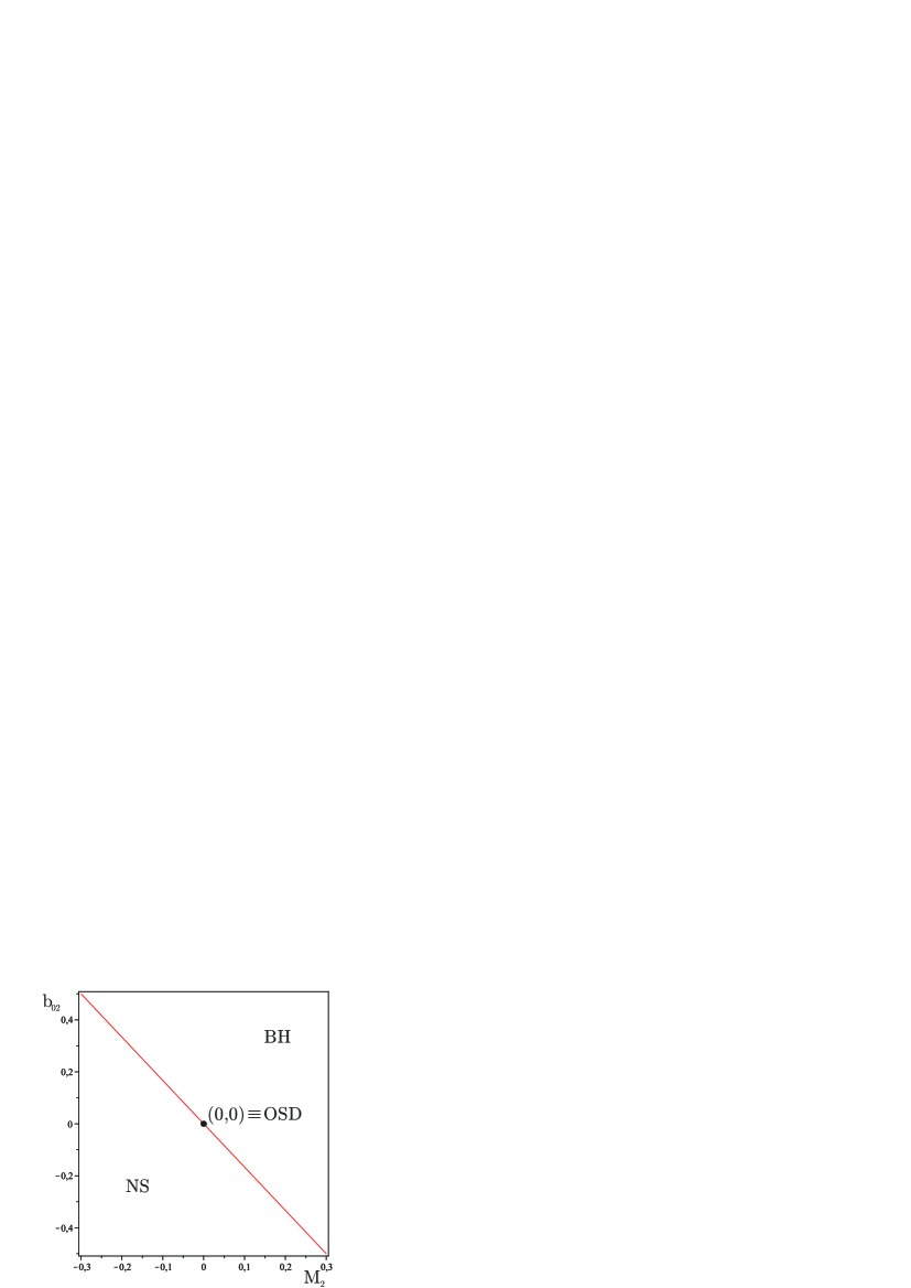
Figure 1: The phase space of initial data for the LTB collapse model with $M_{0}=1$ and $M_{1}=b_{00}=b_{01}=0$. In this case $\chi_{1}=0$ and $\chi_{2}$ determines the final outcome of collapse depending on the values of $M_{2}$ and $b_{02}$. There are initial data sets that have a whole neighborhood leading to the same outcome in terms of either a black hole or naked singularity. The OSD case lies on the critical surface separating the two outcomes which is defined by $\chi_{i}=0$ for all $i$.

For example, in the marginally bound case (namely $b_{0}=0$) the singularity curve for inhomogeneous dust becomes $t_{s}(r)=t_{i}+\frac{2}{3}\frac{1}{\sqrt{M(r)}}$ and the apparent horizon curve is given by $t_{ah}(r)=t_{s}(r)-\frac{2}{3}r^{2}M(r)$ and in general collapse may lead to black hole or naked singularity depending on the behaviour of the mass profile $M(r)$. By writing $M(r)$ near $r=0$ as a series $M(r)=M_{0}+M_{1}r+M_{2}r^{2}+o(r^{3})$ we see that the lowest order non-vanishing $M_{i}$ (with $i>0$) governs the final outcome of collapse. As expected in this case, we have

$$\chi_{1}(0) = -\frac{1}{3}\frac{M_{1}}{M_{0}^{\frac{3}{2}}}\;,$$ (III.2)

$$\chi_{2}(0) = \frac{1}{4}\frac{M_{1}^{2}}{M_{0}^{\frac{5}{2}}}-\frac{1}{3}\frac{M_{2}}{M_{0}^{\frac{3}{2}}}\;.$$ (III.3)

In the perfect fluid LTB model (corresponding to the FRW cosmological models in case of expansion) we have that requiring $v=v(t)$ is a sufficient condition for having homogeneous collapse. In fact the following two statement can be easily proved:

1. $v=v(t)\Leftrightarrow\begin{cases}M(r,t)=M(t)\;,\\ b_{0}(r)=k\;.\end{cases}$

2. $v=v(t)\Rightarrow\begin{cases}\rho=\rho(t)\;,\\ p=p(t)\;.\end{cases}$

The overall behaviour of the collapsing cloud is determined by the three functions $M(r,t)$, $v(r,t)$ and $b_{0}(r)$ (which, as we have seen, are not independent from one another) and the special cases of Oppenheimer-Snyder-Datt metric and Lemaitre-Tolman-Bondi perfect fluid metric can be summarized as follows.

$$\begin{array}[]{ccccc}M_{0},&k,&v(t)&\Leftrightarrow&\text{Homogeneous dust}\\ M(r),&b_{0}(r),&v(r,t)&\Leftrightarrow&\text{Inhomogeneous dust}\\ M(t),&k,&v(t)&\Rightarrow&\text{Homogeneous perfect fluid}\end{array}$$

III.2 Perturbation of inhomogeneous dust

We consider now an example based on the above framework by introducing a small pressure perturbation to the inhomogeneous dust model described in the previous section. We consider in general $v=v(r,t)$ and the mass function is chosen of the form

$$M=M_{0}+M_{2}(v)r^{2}\;,$$ (III.4)

where $M_{0}$ is a constant and the pressure perturbation is taken to be small in the sense that $M_{0}\gg|M_{2}|$ at all times (in this way, as collapse progresses and the density diverges the model remains close to the LTB collapse as the pressure is always smaller than the density). We immediately see that setting $M_{2}=C$ reduces the model to that of inhomogeneous dust (and $C=0$ further gives the OSD homogeneous dust). We note that in this case no non-central singularities are visible since $M$ does not vanish at $v=0$. Therefore, just like in the dust case, only the central singularity at $r=0$ might eventually be visible.

In this case we can integrate equation (II.39) explicitly to obtain

$$A_{2}(v)=\frac{2}{3}\frac{M_{2}(v)-C}{M_{0}}\,,$$ (III.5)

where $C$ now is the value taken by $M_{2}$ at the initial time when $v=1$. Therefore we can take the mass function in such a way that it corresponds to the LTB inhomogeneous dust at initial time with the pressure perturbation being triggered only at a later stage. We can therefore take,

$$M_{2}(v)=C+\epsilon(v)\;,$$ (III.6)

and the initial condition $M_{2}(1)=C$ implies that $\epsilon(1)=0$ (remember that $v\in[0,1]$). By taking all the higher order terms to be vanishing we easily see that $A_{i}=0$ for $i>2$ and

$$g_{0}=\frac{1}{2}A_{2,v}v=\frac{1}{3}\frac{M_{2,v}v}{M_{0}}\;,$$ (III.7)

near $r=0$.

In this case the pressure and the energy density near $r=0$ become

$$p=-\frac{\epsilon_{,v}}{v^{2}}r^{2},\;\rho=\frac{3M_{0}}{v^{3}}+5\frac{C+\epsilon}{v^{3}}r^{2}\;.$$ (III.8)

We therefore have two simple possibilities for the choice of the free function $\epsilon$ which determines $M$:

1. $\epsilon>0$ which implies $\epsilon_{,v}<0$ and positive pressure.

2. $\epsilon<0$ which implies $\epsilon_{,v}>0$ and negative pressure.

From the above, further assuming $b_{0}=0$ for simplicity in accordance with marginally bound LTB models, it follows immediately that $\chi_{1}(0)=0$ and

$$\chi_{2}(0)=-\frac{1}{2}\int^{1}_{0}\frac{(C+H(v))\sqrt{v}}{\left(M_{0}+\frac{4}{3}\frac{\epsilon v}{M_{0}}\right)^{\frac{3}{2}}}dv-\frac{4}{9M_{0}^{2}}\int^{1}_{0}\frac{\epsilon v(\epsilon+\epsilon_{,v}v)\sqrt{v}}{\left(M_{0}+\frac{4}{3}\frac{\epsilon v}{M_{0}}\right)^{\frac{3}{2}}}dv\;,$$ (III.9)

where we defined the function

$$H(v)=\left(\epsilon+\frac{2}{3}\epsilon_{,v}v\right)\;.$$ (III.10)

We see that $\chi_{2}$ is divided into two integrals. If we assume that the pressure perturbation is small (thus considering $M_{0}$ to be big) then the second integral can in principle be neglected. In fact for a suitable choice of $M_{0}$ it is not difficult to prove that the function at the denominator will be positive and monotonically increasing, and therefore it would not affect the sign of the integral, while the second integral will be small enough as compared to the first one. Positivity of $\chi_{2}$ will then be decided by the sign of $C+H(v)$.

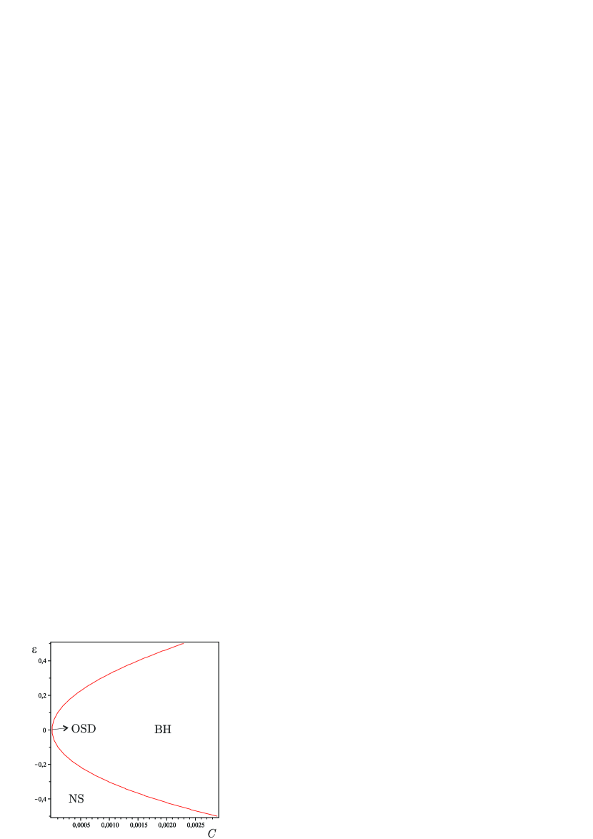
Figure 2: The phase space of initial data for perfect fluid collapse with $M_{0}=1$, $b_{0}=0$ and $M=M_{0}+(C+\epsilon(v))r^{2}$. On the left the pressure is taken to be $p=\varepsilon(3-\frac{2}{v}-\frac{1}{v^{2}})r^{2}$ and it reduces to zero for $\varepsilon=0$. On the right the pressure perturbation is given by $p(r,v)=\left(0.3+\frac{0.2}{v}y-\frac{0.1}{v}\right)r^{2}$. The introduction of the pressure can uncover an otherwise clothed singularity depending on the values of $\varepsilon$, $y$ and $C$. Different choices of $M$ with $\epsilon(v)=y_{0}+y_{1}v+y_{2}v^{2}+y_{3}v^{3}$ will have a similar qualitative behaviour.

In order to have naked singularity we must have $\chi_{2}>0$. This is certainly the case whenever

$$C<-H(v)\;,$$ (III.11)

for any $v$. Therefore if we define $D_{1}=\min\{H(v),v\in[0,1]\}$ all the values of $C<D_{1}$ will lead to a naked singularity. On the other hand, values of $C>D_{2}=\max\{H(v),v\in[0,1]\}$ will lead to the formation of a black hole. For $C\in[D_{1},D_{2}]$ the explicit form of $\epsilon(v)$ is what determines the sign of $\chi_{2}$. It can be proven that we can have models in which positive values of $C$ lead to the formation of a naked singularity whereas the inhomogeneous dust case led to a black hole.

III.3 A perturbation with pressure $\bf{p(r)}$

We now analyze another case where the pressure perturbation introduced does not depend explicitly on $v$. A similar situation was investigated by one of us earlier in Sar-Pramana . Here we consider a pressure perturbation of LTB models of the form $p=p(r)$.

If we impose

$$M_{,vv}v-2M_{,v}=0\;,$$ (III.12)

in the equation (II.35), we can then solve for $M$ and explicitly evaluate $G$. We obtain in that case,

$$M(r,v)=y(r)v^{3}+z(r)\;,$$ (III.13)

where $y(r)$ and $z(r)$ come from integration. Here the case where $y=0$ reduces the system to dust. In this sense, if we keep $|y|\ll z$ we will consider this model to be a small perturbation of LTB in a similar way as was discussed in the previous example. Then the radial derivatives of $z$ will correspond to the inhomogeneities in the LTB models while the pressure, or the function $y$, can be taken to be either positive or negative (with positive pressure corresponding to an increasing mass function $M$ and negative pressure corresponding to a decreasing mass function).

In order to work on a specific model for the sake of clarity, we assume that $y$ and $z$ can be expanded near the center as,

$$y(r) = y_{0}+y_{1}r+y_{2}r^{2}+...\;,$$ (III.14)

$$z(r) = z_{0}+z_{1}r+z_{2}r^{2}+...\;.$$ (III.15)

Then the pressure and density become

$$p=-3y(r),\;\rho=\frac{3z+z_{,r}r+y_{,r}rv^{3}}{v^{2}R^{\prime}}-p\;.$$ (III.16)

Imposing regularity requires that $y_{,r}(0)=z_{,r}(0)=0$, which implies $y_{1}=z_{1}=0$. At the center of the cloud the pressure and density become $p_{0}=-3y_{0}$ and $\rho_{0}=3\left(\frac{z_{0}}{v^{3}}+y_{0}\right)$, and the energy conditions impose that $z_{0}\geq 0$ and $y_{0}\geq-z_{0}$. Then from equation (II.36) we can integrate explicitly to obtain,

$$A(r,v)=\ln\left(\frac{u(r)+1}{u(r)+v^{3}}\right)\;,$$ (III.17)

where we have defined

$$u(r)\equiv\frac{3z(r)+z_{,r}r}{y_{,r}r}\;.$$ (III.18)

Then we get,

$$G(r,v)=b(r)\left(\frac{u+1}{u+v^{3}}\right)^{2}\;.$$ (III.19)

From the above expressions, we can easily obtain now $\chi_{1}$ and $\chi_{2}$. For simplicity we consider here the case where $b_{0}=y_{4}=0$. Then $\chi_{1}=0$ and we get,

$$\chi_{2}=-\frac{1}{2}\int^{1}_{0}\left[\frac{2\frac{y_{2}}{z_{0}}v^{6}}{\sqrt{y_{0}v^{3}+z_{0}+\frac{4}{3}\frac{y_{2}}{z_{0}}v(1-v^{3})}}+\frac{y_{2}v^{3}+z_{2}+\frac{1}{3}\frac{y_{2}}{z_{0}^{2}}v(v^{3}-1)\left[y_{2}(v^{3}-\frac{1}{3})+\frac{5}{3}z_{2}\right]}{\left(y_{0}v^{3}+z_{0}+\frac{4}{3}\frac{y_{2}}{z_{0}}v(1-v^{3})\right)^{\frac{3}{2}}}\right]\sqrt{v}dv$$ (III.20)

We see from here that the sign of $\chi_{2}$ is explicitly determined by the inhomogeneities ($z_{2}$) and the pressure gradient ($y_{2}$) (see Fig.3).

Once again taking $y_{0}=y_{2}=0$ and $z_{2}=0$ reduces the system to the OSD collapse scenario and we see that the introduction of the slightest pressure can change drastically the outcome of collapse. On the other hand, taking only $y_{0}=y_{2}=0$ (with $z_{2}\neq 0$) we retrieve the LTB model and once again to change the final outcome of collapse we must choose $y_{2}$ suitably to balance the contribution to $\chi_{2}$ given by the inhomogeneities. Therefore we see again that also within this perturbation model any collapse with initial data taken in a neighborhood of a model leading to a certain outcome and not lying on the critical surface will result in the same endstate.

The equation for the apparent horizon curve can be easily written in this case and becomes

$$r^{2}y(r)v_{ah}(r)^{3}-v_{ah}(r)+r^{2}z(r)=0\;,$$ (III.21)

which is a cubic equation in $v_{ah}$ that admits in general three solutions in the case where $27r^{4}z^{2}-\frac{4}{r^{2}y}\geq 0$. Obviously this condition is satisfied near $r=0$ for positive pressures (that correspond to negative $y$) and this indicates, as already stated, that the mass function is not vanishing at any time and therefore the central shell becomes trapped at the time of formation of the singularity. On the other hand, for negative pressures the central shell is not trapped and the formation of the apparent horizon can be shifted to some outer shells or removed altogether.

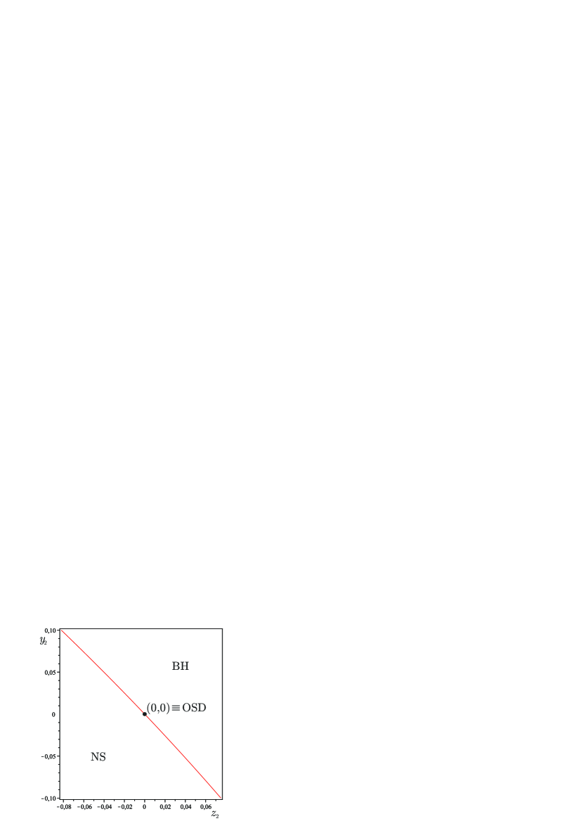
Figure 3: The numerical evaluation of the sign of $\chi_{2}$ as a function of $y_{2}$ and $z_{2}$ provides the phase space of initial data for the perfect fluid model with $p=p(r)$. Here we have taken $z_{0}=1$ and $y_{0}=-1/2$. Again, there are initial data sets that have a whole neighborhood leading to the same outcome which is either a black hole or naked singularity. The OSD case lies on the critical surface separating the black holes from naked singularities.

III.4 Perturbation of a general simultaneous collapse

As we mentioned, the case of simultaneous collapse, which means that the final state of collapse is necessarily a black hole, need not be restricted to the Oppenheimer-Snyder-Datt model only. In fact for different kinds of general type I matter fields there might be suitable choices of the parameters that lead the final state of collapse to be simultaneous. This is of course the case when the pressures are homogeneous, that is represented by the time reversal of the Friedman-Robertson-Walker model, but more general matter models might also lead to the same behaviour.

Simultaneous collapse means that all matter shells terminate into the singularity at the same time. Then we see from equation (II.46), which describes the singularity curve, that all coefficients $\chi_{i}(0)$ must vanish, or equivalently that $t_{s}(r)=t_{0}$. From equation (II.43) we can see that a sufficient condition for simultaneous collapse is

$$\frac{e^{-2\nu}}{\frac{M}{v}+\frac{be^{2A}-1}{r^{2}}}=h(v)\;.$$ (III.22)

This condition, for any given choice of the matter model, leads to a choice of the free function $b(r)$ as

$$b(r)=e^{-2A}\left(1+\frac{e^{-2\nu}}{h}r^{2}-\frac{M}{v}r^{2}\right)\;.$$ (III.23)

It is easy to check that in the case of dust this reduces to

$$b_{0}(r)=\frac{1}{h(v)}-\frac{M(r)}{v}\;,$$ (III.24)

and since the mass profile in this case is a function of $r$ only, we conclude that equation (III.22) is satisfied for dust only by the case of homogeneous dust collapse (where $M(r)=M_{0}$ and $b_{0}=k$). Nevertheless, as we have said, this need not be the only case when the collapse is simultaneous. For example it’s straightforward to see that when pressures are considered, the same condition as above holds for collapse of an homogeneous perfect fluid, where, in this case, $M=M(t)$. Furthermore it is possible that the condition (III.22) can be satisfied by some suitable function $b(r)$ also for more general pressure profiles, since in general the mass function depends on both $r$ and $t$, or for some other suitable choice of the velocity profile.

In order to better understand the conditions under which we can have simultaneous collapse in full generality, let us now consider a general perfect fluid matter model given by a choice of $M(r,v)$ (which implies $A$ from equation (II.36)), thus specifying all coefficients $M_{i}(v)$. Firstly, we notice from equation (II.45) that a suitable choice of $b_{00}$ is necessary in order for the reality condition to be fulfilled near the center. Therefore, once we made this choice and carried out the integration for equation (II.47) we see that $\chi_{1}(0)$ depends linearly on $b_{01}$ only. In fact we can write

$$\chi_{1}(0)=-\frac{1}{2}\int_{0}^{1}\alpha_{1}(v)dv-\frac{b_{01}}{2}\int^{1}_{0}\beta_{1}(v)dv\;,$$ (III.25)

from which we see that it will always be possible to choose $b_{01}$ suitably such that $\chi_{1}(0)=0$. The same reasoning can then be applied for all other coefficients $\chi_{i}(0)$ that will depend linearly on $b_{0i}$ as,

$$\chi_{i}(0)=\int_{0}^{1}\alpha_{i}(v)dv+b_{0i}\int^{1}_{0}\beta_{i}(v)dv\;,$$ (III.26)

and therefore for a given mass profile $M(r,v)$ we can have simultaneous collapse if a suitable velocity profile $b(r)$ given by

$$b(r)=1+r^{2}\sum_{i=0}^{\infty}\frac{b_{0i}}{i!}r^{i}\;,$$ (III.27)

exists. This means that the power series $\sum_{i=0}^{\infty}\frac{b_{0i}}{i!}r^{i}$ should converge to some function $b_{0}(r)$ with a radius of convergence greater than the boundary of the cloud.

This is certainly possible in the case of homogeneous pressures, where the condition that all $\chi_{i}(0)$ vanish imposes that $\sum_{i=0}^{\infty}\frac{b_{0i}}{i!}r^{i}=\frac{C}{r2}$, and therefore $b(r)=const$. Also, as we have seen in the examples above, this might be possible for other matter profiles as well. Given any such model leading to simultaneous collapse (and thus to the formation of a black hole), we have shown that the introduction of the slightest pressure perturbation in the initial data can turn the final outcome into a naked singularity.

Overall we have seen that the sign of $\chi_{2}$ and therefore the final outcome of collapse shares similar qualitative behaviour in different perfect fluid models as it is summarized in Fig. 4.

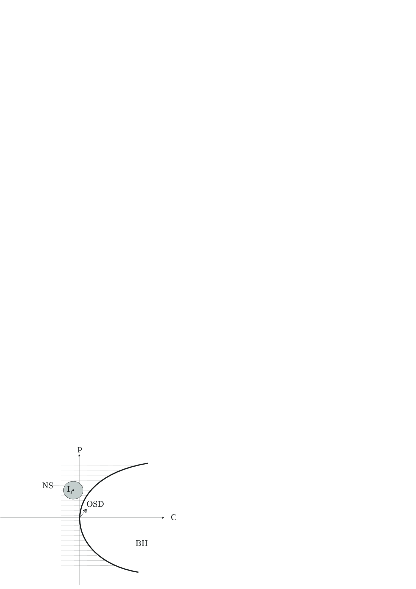
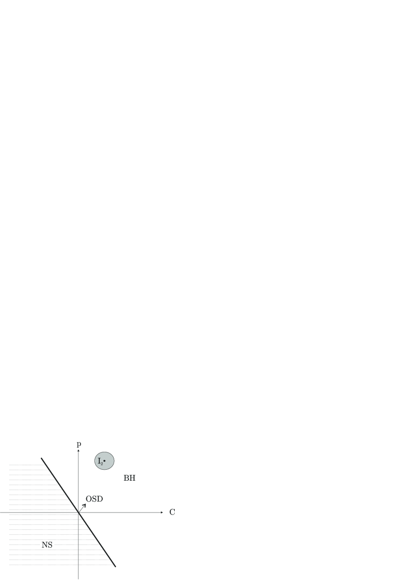
Figure 4: Illustrative representation of the phase spaces of initial data for different perfect fluid collapse models with assigned mass profiles $M(r,v)$ and with $b_{0}=0$. The introduction of pressures $p$ and inhomogeneities $C$ can uncover an otherwise clothed singularity. Also, different choices of $M$ can have the opposite effect, that is, a singularity that was naked can become covered. The initial data set $\emph{I}_{1}$ has a whole neighborhood lying in the initial data space leading to naked singularity and can therefore be considered stable. The same holds for the initial data set $\emph{I}_{2}$ leading to black hole. The LTB model (obtained for $p=0$ and) can lead to either of the outcomes and the OSD scenario (obtained when there are no inhomogeneities) always lies on the critical surface separating the two outcomes and is therefore ‘unstable’.

IV Genericity of black holes and naked singularities

As we have seen, the final outcome of collapse depends upon the evolution of the pressure, the density and the velocity profiles. If the system is closed, as it is in the case where an equation of state describing the relation between $p$ and $\rho$ is given, then specifying the values of the above quantities at the initial time uniquely determines the final outcome of collapse. If the system is not closed, then we must further specify the behaviour of the free functions. Once again for every possible choice of the free function(s) the final outcome of collapse is decided by the initial values of $p$, $\rho$ and $b$.

The genericity is defined here as every point in the initial data set leading to a naked singularity (or a black hole) has a neighborhood in the space of initial data for collapse whose points all lead to the same outcome. We show that the initial data set leading the collapse to a naked singularity forms an open subset of a suitable function space comprising of the initial data, with respect to an appropriate norm which makes the function space an infinite dimensional Banach space. The measure theoretic aspects of this open set are considered and we argue that a suitable well-defined measure of this set must be strictly positive. This ensures genericity of initial data in a well-defined manner.

At this point, the question of whether the given outcome is ‘generic’ or not in a certain suitable sense yet to be defined, with respect to the allowed initial data sets, arises naturally. We shall therefore analyze the expression (II.47) for the genericity of initial data leading the collapse to a naked singularity. Similar conclusions apply to the case where $\chi_{1}$ vanishes and we must analyze equation (II.48) and they can be used to investigate the genericity of the black hole formation scenario just as well.

As is known the concept of ‘genericity’ is not well-defined in General Relativity. Normally, by the word ‘generic’, one means ‘in abundance’ or ‘substantially big’. This terminology has been used by many researcher working in relativity, and in gravitational collapse in particular (see for example, genericity1 -genericity3 ). In the theory of Dynamical Systems, however, the definition of ‘genericity’ is given more tightly. There, one considers the class $\mathrm{V}$ of all $\mathcal{C}^{r}$ vector fields (dynamical systems) defined on a given manifold. A property $\mathrm{P}$ satisfied by a vector field $X$ in $\mathrm{V}$ is called generic if the set of all vector fields satisfying this property contains an open and dense subset of $\mathrm{V}$. This was the definition used by one of us in Sar-Pramana and SG . However, such a definition would render both black holes and naked singularities to be ‘non-generic’, as we remarked earlier. Therefore in the present paper we have opted for a less stringent but physically more meaningful definition of genericity by requiring that the subset is open, and that it has a non-zero measure. The main reason for this comes from the fact that the ‘denseness’ property depends on the topology used and the parent space used, and there are no unique and unambiguous definitions available in this regard as discussed earlier. Hence the nomenclature of ‘generic’ in the present paper is used in the sense in which most of the relativists use it, i.e. in the sense of abundance. This looks physically more satisfactory definition, allowing both black holes and naked singularities to be generic. In any case, the key point is that regardless of the definition used, both the collapse outcomes do share the same ‘genericity’ properties, which is what our work here shows.

IV.1 Existence of the set of initial data leading to naked singularity

First of all we note that the functions must satisfy the ‘reality condition’ for the gravitational collapse to take place, namely

$$\frac{M_{0}(v)}{v}+b_{0}(0)+2a(0,v)>0\;,$$ (IV.1)

where we have defined $a(r,v)\equiv\frac{A(r,v)}{r^{2}}$.

We shall now prove that, given a mass function $M(r,v)$, and the function $a(r,v)$ on the initial surface, there exists a large class of velocity distribution functions $b_{0}(r)$ such that the final outcome is a naked singularity. We choose $b_{0}(r)$ to satisfy the following differential equation on a constant $v$-surface,

$$\frac{1}{2}\frac{\frac{M^{\prime}(r,v)}{v}+b_{0}^{{{}^{\prime}}}(r)+2a^{\prime}(r,v)}{\left[\frac{M(r,v)}{v}+b_{0}(r)+2a(r,v)\right]^{\frac{3}{2}}}=B(r,v)\;,$$ (IV.2)

for $0\leq r\leq r_{b}$, where $B(r,v)$ is a continuous function defined on a domain $D=[0,r_{b}]\times[0,1]$ such that

$$B(0,v)=\frac{1}{2}\frac{\frac{M^{\prime}(0,v)}{v}+b_{0}^{{{}^{\prime}}}(0)+2a^{\prime}(0,v)}{\left[\frac{M(0,v)}{v}+b_{0}(0)+2a(0,v)\right]^{\frac{3}{2}}}<0\;,$$ (IV.3)

for all $v\in[0,1]$. It will then follow that

$$\chi_{1}(0)=\lim_{v\to 0}\chi_{1}(v)=-\int_{0}^{1}B(0,v)dv>0\;.$$ (IV.4)

As seen above, this condition ensures that central shell-focusing singularity will be naked.

We prove the existence of $b_{0}(r)$ as a solution of the differential equation (IV.2) with initial condition (IV.3) which $B(r,v)$ will satisfy. For this purpose, we define

$$x(r,v)=M(r,v)+vb_{0}(r)+2va(r,v)\;.$$ (IV.5)

Then equation (IV.2) can be written as

$$\frac{\sqrt{v}}{2}\frac{\left[M^{\prime}(r,v)+vb_{0}^{\prime}(r)+2va^{\prime}(r,v)\right]}{\left[M(r,v)+vb_{0}(r)+2va(r,v)\right]^{\frac{3}{2}}}=\frac{1}{2}\sqrt{v}\frac{\frac{dx}{dr}}{x^{\frac{3}{2}}}=B(r,v)\;,$$ (IV.6)

or

$$\frac{dx}{dr}=\frac{1}{\sqrt{v}}\left[2B(r,v)x^{\frac{3}{2}}\;,\right]\equiv f(x,r)\;,$$ (IV.7)

with the initial condition

$$x(0,v)=M_{0}(v)+vb_{0}(0)+2va(0,v)\;.$$ (IV.8)

We now ensure the existence of a $\mathcal{C}^{1}$-function $x(r,v)$ as a solution of the above initial value problem defined throughout the cloud. The function $f(x,r)$ is continuous in $r$, with $x$ restricted to a bounded domain. With such domain of $r$ and $x$, $f(x,r)$ is also a $\mathcal{C}^{1}$-function in $x$ which means $f(x,r)$ is Lipschitz continuous in $x$. Therefore, the differential equation (IV.7) has a unique solution satisfying the initial condition (IV.8), provided $f(x,r)$ satisfies a certain condition given below.

Further, we can ensure that the solution will be defined over the entire cloud, i.e. for all $r\in[0,r_{b}]$, by using the freedom in the choice of arbitrary function $B(r,v)$. For this, we consider the domain $[0,r_{b}]\times[0,d]$ for some finite $d$.

Let us take $S=\sup\left|f(x,r)\right|$. Then the differential equation (IV.7) has a unique solution defined over the entire cloud provided,

$$r_{b}\leq\inf(r_{b},\frac{d}{S})=\frac{d}{S}\;.$$ (IV.9)

This condition is to be satisfied according to usual existence theorems to guarantee existence of a unique solution (see for example gen1 ). Equation (IV.9) implies $S\leq\frac{d}{r_{b}}$ i.e.,

$$\mathop{\max}\limits_{0\leq r\leq r_{b,},0\leq v\leq d}\left|\frac{1}{\sqrt{v}}\left[2B(r,v)x^{\frac{3}{2}}\right]\right|\leq\frac{d}{r_{b}}\;.$$ (IV.10)

This, in turn, will be satisfied if

$$0\leq\left|B(r,v)x^{\frac{3}{2}}\right|\leq\frac{d\sqrt{v}}{2r_{b}}\;,$$ (IV.11)

for all $r\in[0,r_{b}]$.

The collapsing cloud may start with $r_{b}$ small enough so that the expression $\frac{d\sqrt{v}}{2r_{b}}$ which is always positive, satisfies the condition (IV.11) with $x$ restricted to a bounded domain. We then have infinitely many choices for the function $B(r,v)$, which is continuous and satisfies conditions (IV.3) and (IV.11) for each choice of $v$. For each such $B(r,v)$, there will be a unique solution $x(r,v)$ of the differential equation (IV.7), satisfying initial condition (IV.8), defined over the entire cloud, and in turn, there exists a unique function $b_{0}(r)$ for each such choice of $B(r,v)$, that is given by the expression

$$b_{0}(r)=\frac{x(r,v)-M(r,v)-2va(r,v)}{v}\;.$$ (IV.12)

Thus, we have shown the following: For a given constant $v$-surface and given initial data of mass function $F(t,r)=r^{3}M(r,v)$ and $a(r,v)$ satisfying physically reasonable conditions (expressed on $M$), there exists infinitely many choices for the function $b(r)$ such that the condition (IV.2) is satisfied. The condition continues to hold as $v\rightarrow 0$, because of continuity. Hence, for all these configurations the central singularity developed in the collapse is a naked singularity.

The above analysis shows that the initial data satisfying conditions (IV.1), (IV.3) and (IV.11) lead the collapse to a naked singularity. If we change the sign in condition (IV.3), call it condition (IV.3)^′, then above analysis apply and the initial data satisfying conditions (IV.1), (IV.3)^′ and (IV.11) lead the collapse to a black hole. In the cases discussed above, in addition to above conditions, energy conditions are also to be satisfied, and we have shown above that this is always possible for matter models leading to both possible outcomes.

Thus, from the above analysis, we get the following conditions which should be satisfied by the initial data in order that the end state of collapse is a naked singularity:

1. Energy conditions: $\rho\geq 0$ , and $\rho+p\geq 0$.

2. Reality condition given by equation (IV.1) above.

3. Condition on $B(r,v)$: $B(0,v)<0$ for naked singularity and $B(0,v)>0$ for black hole.

4. $0\leq$ $\left|B(r,v)x^{\frac{3}{2}}\right|\leq\frac{d\sqrt{v}}{2r_{b}}$.

For convenience, we denote the function

$$C(r,v)=\frac{M(r,v)}{v}+b_{0}(r)+2a(r,v)\;.$$

Then the reality condition (2) becomes $C(0,v)>0$. Assuming this condition, condition (3) will be satisfied if and only if $\frac{M^{\prime}(0)}{v}+b_{0}^{{{}^{\prime}}}(0)+2a^{\prime}(0,v)<0$ for naked singularity, and $>$ 0 for a black hole. Whenever $C(r,v)$ is an increasing function of $r$ in the neighborhood of $0$, we get its derivative positive, and so $B(0,v)>0$, and end state will be a black hole. On the other hand, if $C(r,v)$ is a decreasing function of $r$ in the neighborhood of $0$, we get its derivative negative, and so $B(0,v)<0$, and the endstate will be a naked singularity.

Regarding condition (4), using the expression $x=vC(r,v)$, it becomes $C^{\prime}(r,v)\leq\frac{d}{vr_{b}}$ which will be satisfied if $v$ and $r_{b}$ are sufficiently small. Thus validity of all these conditions does not put any stringent restrictions on the initial data.

The conclusion then is the following: If the initial data consisting of the mass function $M(r,v)$ and function $a(r,v)$ satisfies the above conditions, then there is a large class of velocity functions $b_{0}(r)$ such that end state of collapse is either a black hole or a naked singularity, depending on the nature of function $C(r,v)$ as explained above.

IV.2 Measure of the set of initial data leading to naked singularity

We now show that the set of initial data $\mathcal{G}=\{M(r,v),a(r,v),b(r)\}$ satisfying the above conditions which lead the collapse to a naked singularity, is an open subset of $X\times X\times X$, where $X$ is an infinite dimensional Banach space of all $\mathcal{C}^{1}$ or $\mathcal{C}^{2}$ real-valued functions defined on $\mathcal{D}=[0,r_{b}]\times[0,d]$, endowed with the norms

$$\parallel\textit{M}(r,v)\parallel_{1} = \sup_{{\mathcal{D}}}|\textit{M}|+\sup_{{\mathcal{D}}}|\textit{M}_{,r}|+\sup_{{\mathcal{D}}}|\textit{M}_{,v}|\;,$$ (IV.13)

$$\parallel\textit{M}(r,v)\parallel_{2} = \parallel\textit{M}(r,v)\parallel_{1}+\sup_{{\mathcal{D}}}|\textit{M}_{,rr}|+\sup_{{\mathcal{D}}}|\textit{M}_{,rv}|+\sup_{{\mathcal{D}}}|\textit{M}_{,vv}|\;.$$ (IV.14)

These norms are equivalent to the standard $\mathcal{C}^{1}$ and $\mathcal{C}^{2}$ norms,

$$\parallel\textit{M}(r,v)\parallel_{1} = \sup_{{\mathcal{D}}}(|\textit{M}|+|\textit{M}_{,r}|+|\textit{M}_{,v}|)\;,$$ (IV.15)

$$\parallel\textit{M}(r,v)\parallel_{2} = \sup_{{\mathcal{D}}}(\parallel\textit{M}(r,v)\parallel_{1}|+|\textit{M}_{,rr}|+|\textit{M}_{,rv}|+|\textit{M}_{,vv}|)\;.$$ (IV.16)

Let ${\mathcal{G}_{1}}=\{M(r,v):M>0,M\text{ is }\mathcal{C}^{1},\ E_{1}>0\text{ and }E_{2}>0\text{ on }\mathcal{D}\}$ be a subset of $X$, where $E_{1}=3M+rM_{,r}+rv^{\prime}M_{,v}$ and $E_{2}=3M+rM_{,r}-vM_{,v}$. Thus $E_{1}>0$ and $E_{2}>0$ are equivalent to energy conditions.

We first show that $\mathcal{G}_{1}$ is an open subset of $X$. For simplicity, we use the $\mathcal{C}^{1}$ norm, but a similar proof holds for the $\mathcal{C}^{2}$ norm also. For $M\in\mathcal{G}_{1}$, let us put $\delta=\min(M)$, $\gamma=\min(E_{1})$ , $\beta=\min(E_{2})$, $\lambda_{1}=\max(v)$, $\lambda_{2}=\max(v^{\prime})$ and for $r$ varying in $[0,r_{b}]$ and $v\in[0,1]$, the functions involved herein are all continuous functions defined on a compact domain $\mathcal{D}$ and hence, their maxima and minima exist. We define a positive real number

$$\mu=\frac{1}{2}\min\{\delta,\frac{\gamma}{9},\frac{\gamma}{3r_{b}},\frac{\gamma}{3r_{b}\lambda_{2}},\frac{\beta}{9},\frac{\beta}{3r_{b}},\frac{\beta}{3\lambda_{1}}\}.$$ (IV.17)

Let $M_{1}(r,v)$ be $\mathcal{C}^{1}$ in $\mathcal{D}$ with $\parallel M-M_{1}\parallel_{1}<\mu$. Using above definition we get $|M_{1}-M|<\mu$, $|M_{1,r}-M_{,r}|<\mu$, $|M_{1,v}-M_{,v}|<\mu$ over $\mathcal{D}$. Therefore, for choice of $\mu$, the respective inequalities are

$$M_{1} > M-\frac{\delta}{2}>0,$$ (IV.18)

$$3|M_{1}-M| < \frac{\gamma}{6},$$

$$r|M_{1,r}-M_{,r}| \leq r_{b}|M_{1,r}-M_{,r}|<\frac{\gamma}{6},$$

$$rv^{\prime}|M_{1,v}-M_{,v}| \leq r_{b}\lambda_{2}|M_{1,v}-M_{,v}|<\frac{\gamma}{6},$$

$$3|M_{1}-M| < \frac{\beta}{6},$$

$$r|M_{1,r}-M_{,r}| < \frac{\beta}{6},$$

$$v|M_{1,v}-M_{,v}| \leq r_{b}|M_{1,v}-M_{,v}|<\frac{\beta}{6},$$

that are satisfied on ${\mathcal{D}}$. The $2^{nd}$ , $3^{rd}$ and $4^{th}$ inequalities from above yield

$$3|\textit{M}_{1}-\textit{M}|+r|\textit{M}_{1,r}-\textit{M}_{,r}|+rv^{\prime}|\textit{M}_{1,v}-\textit{M}_{,v}|<\frac{\gamma}{2}<{\gamma}\leq E_{1}\;.$$ (IV.19)

Further, we can write $|[3M_{1}+rM_{1,r}+rv^{\prime}M_{1,v}]-E_{1}|<E_{1}$ where $E_{1}>0$ on $\mathcal{D}$.

Hence, $3M_{1}+rM_{1,r}+rv^{\prime}M_{1,v}>0$ on $\mathcal{D}$. Using similar analysis for last four inequalities of equation (IV.18), we obtain $3M_{1}+rM_{1,r}-vM_{1,v}>0$ on $\mathcal{D}$.

Thus, $M_{1}>0$, $M_{1}$ is $\mathcal{C}^{1}$ , $[3M_{1}+rM_{1,r}+rv^{\prime}M_{1,v}]>0$ and $[3M_{1}+rM_{1,r}-vM_{1,v}]>0$ on ${\mathcal{D}}$  provided $v>0$ throughout ${\mathcal{D}}$. Therefore, $M_{1}(r,v)$ also lies in ${\mathcal{G}_{1}}$  and hence, ${\mathcal{G}_{1}}$ is an open subset of $X$.

Using the similar argument we can show that the set $\mathcal{G}_{2}=\{M(r,v):|B(r,v)|x^{\frac{3}{2}}<\frac{d\sqrt{v}}{2r_{b}}\}$ is also an open subset of $X$. Thus the set of $M(r,v)$ satisfying above conditions forms an open subset of $X$, since intersection of finite number of open sets is open. Similar arguments show that the set of $a(r,v)$ and $b(r)$ satisfying these conditions form separately open subsets of $X$. Hence using definition of product topology we see that the set $\mathcal{G}$ defined above is an open subset of $X\times X\times X$. Thus initial data leading the collapse to a naked singularity forms an open subset of the Banach space of all possible initial data, and therefore it is generic.

We now discuss measure theoretic properties of the open set $\mathcal{G}$ consisting of the initial data leading the collapse to a naked singularity. By referring to the relevant literature about measures on infinite dimensional separable Banach spaces, we argue that this $\mathcal{G}$ has strictly positive measure in an appropriate sense. For simplicity, we consider a single space $X$ and its open subset $\mathcal{G}$. We ask the question: Does there exist a measure on $X$ which takes positive value on $\mathcal{G}$? To answer this question, we note that $X$ is an infinite dimensional separable Banach space, and it is a consequence of Riesz lemma in functional analysis that every open ball in $X$ contains an infinite disjoint sequence of smaller open balls. So, if we want a translation invariant measure on $X$  then its value will be same on each of these balls. Thus, if we demand that the surrounding ball has finite measure, then each of these smaller balls will have measure zero. Otherwise sum of their measures would be infinite by countable additivity. In other words, for separable Banach spaces, every open set has either measure zero or infinite under a translation invariant measure. So, if we wish to have a non-trivial measure on $X$, then we have to discard the property of translation invariance. In that case we must shift to Gaussian measures or Wiener measures. Under these measures, we can conclude that an open subset of $X$ will have a positive measure. For example, it is proved in gen2 (Theorem 2 on page 159), that Gaussian measure of an open ball in a separable Banach space is positive. We can also use Wiener measure on $\mathcal{C}([0,1])$to get the same result (see for example gen3 and gen4 ).

However, for all practical purposes in Physics and Astrophysics, physical functions could be assumed to be Taylor expandable. Thus assuming that our initial data is regular and Taylor expandable, and again working for simplicity with a single function space, instead of product space, we can formulate our problem of measure as follows: Let $Y$ denote the space of Taylor expandable functions defined on an interval $[0,T]$. We consider initial data consisting of functions with first finite number of terms, say $n$ terms, which lead the collapse to a naked singularity. These functions will belong to a finite dimensional space isomorphic to $\mathbb{R}^{n}$. Working with supremum norm as above and arguing similarly, we can prove that the initial data set satisfying conditions (1) to (4) above is an open subset of $\mathbb{R}^{n}$. Now, we have a standard result (see for example gen5 , prop. 4.3.4, page 83) that a Lebesgue measure of an open subset in $\mathbb{R}^{n}$ is strictly positive. Denoting this measure by $\mu_{n}$ and the open set by $\mathcal{G}_{n}$, we get $\mu_{n}(\mathcal{G}_{n})>0$. If, further, $\mathcal{G}_{n}$ is bounded, then $\mu_{n}(\mathcal{G}_{n})$ will be finite. Hence normalized Lebesgue measure of an open subset, and in particular, of an open ball in $\mathbb{R}^{n}$ is also strictly positive, and in fact bounded. We ask the question: Assuming that $\mu_{n}(\mathcal{G}_{n})>0$, can we get a measure on $Y$ such that measure of $\mathcal{G}$ is positive? This is answered affirmatively by Maxwell-Poincarè theorem which is stated as follows (see for example gen6 ):
Consider the sequence of the normalized Lebesgue measures on the Euclidean spheres $S_{r_{n}}^{n-1}\subset{\mathbb{R}}^{n}$ of radius $r_{n}=c\sqrt{n},c>0$ and the limit of spaces

$${\mathbb{R}}^{1}\subset{\mathbb{R}}^{2}...\subset{\mathbb{R}}^{n}\subset...\subset{\mathbb{R}}^{\infty}\;.$$

Then the weak limit of these measures is the standard Gaussian measure $\mu$ which is the infinite product of the identical Gaussian measures on the line with zero mean and variance $c^{2}$. Thus the limit exists and is positive on an open subset $\mathcal{G}$.

It is also possible to give other approaches which answers affirmatively the existence of such limits which are termed as infinite products or in general ‘projective limits’. We describe briefly one such approach as described by Yamasaki gen7 (For general concepts on measure theory, we refer to gen8 ).
Let $\mathbb{R}^{\infty}$ denote the infinite product of real lines. Let $\mathbb{R}_{0}^{\infty}$ be the subspace of $\mathbb{R}^{\infty}$ given by $\mathbb{R}_{0}^{\infty}=\{(\xi_{n})$: there exists $N$ with $\xi_{n}=0$ for $n\geq N\}$. Then $\mathbb{R}^{\infty}$ is the algebraic dual of $\mathbb{R}_{0}^{\infty}$ and ${\mathcal{B}}_{\mathbb{R}_{0}^{\infty}}$ is the weak Borel field of $\mathbb{R}^{\infty}$. Members of ${\mathcal{B}}_{\mathbb{R}_{0}^{\infty}}$ are called weak Borel subsets of $\mathbb{R}^{\infty}$. The space $Y$ mentioned above can be seen isomorphic to a subspace of $\mathbb{R}^{\infty}$, and is isomorphic to $\mathbb{R}_{0}^{\infty}$ if we consider a finite number of terms in the Taylor expansion. Let $m$ denote one dimensional Lebesgue measure on $\mathbb{R}$. Let $G=(G_{k})$ be a sequence of Borel sets of $\mathbb{R}$ such that $0<m(G_{k})<\infty$. We shall define two Borel measures $m_{k}$ and $\lambda_{k}$ by

$$m_{k}(B)=m(B)/m(G_{k}),\;\lambda_{k}(B)=m_{k}(B\cap G_{k}),$$

$m_{k}$ is $\sigma$-finite, whereas $\lambda_{k}$ is a probability measure on $\mathbb{R}$.

Consider the product measure

$$\mu_{G}^{(n)}=\prod_{k=1}^{n}m_{k}\times\prod_{k=n+1}^{\infty}\lambda_{k}\;,$$

then $\mu_{G}^{(n)}$ is $\sigma$-finite on $\mathbb{R}^{\infty}$.
Then we have the following theorem: For every weak Borel set $E$ of $\mathbb{R}^{\infty}$, put

$$\mu_{G}^{(E)}=\lim_{n\rightarrow\infty}\mu_{G}^{(n)}(E).$$

This limit always exists and becomes a $\sigma$-finite $\mathbb{R}_{0}^{\infty}$-invariant measure on $\mathbb{R}^{\infty}$. Then $\mu_{G}$ lies on

$$L(G)=\cup_{n=1}^{\infty}L_{n}(G),$$

where

$$L_{n}(G)=\mathbb{R}^{n}\times\prod_{k=n+1}^{\infty}G_{k}\;.$$

We note that the measure $\mu_{G}$ defined in this theorem is called the infinite dimensional Lebesgue measure supported by $L(G)$.

For any open bounded subset $E$ of $\mathbb{R}^{\infty}$, $E$ is a Borel set and hence a weak Borel set. Moreover

$$\mu_{G}^{(n)}(E)=\left(\prod_{k=1}^{n}m_{k}\times\prod_{k=n+1}^{\infty}\lambda_{k}\right)(E)=\left(\prod_{k=1}^{n}m_{k}\right)(E)\times\left(\prod_{k=n+1}^{\infty}\lambda_{k}\right)(E)\;,$$

and both these factors are finite. Thus the measure $\mu_{G}$ takes a non-zero value on an open bounded subset $E$ of $\mathbb{R}^{\infty}$. We can employ this measure instead of the Gaussian measure mentioned in Maxwell-Poincarè theorem to yield the desired result. In any case, use of probability measure is inevitable and we conclude that the space of initial data leading to a certain outcome (be it black hole or naked singularity), within a specific collapse scenario has non zero measure with respect to the set of all possible initial data.

V Equation of state

As is known the presence of an equation of state introduces a differential relation for the previously considered free function that closes the system of Einstein equations. Examples of simple, astrophysically relevant, linear and polytropic equations of states are discussed below.

In the scenario described above, the relation between the density and pressure could vary during collapse, as it is natural to assume in the case where we go from a nearly Newtonian initial state to a final state where a very strong gravitational field is present. The equation relating $p$ to $\rho$ will therefore be represented by some function of $r$ and $v$ that is related to the choice of the free function $M$. There are at present many indications that suggest how in the presence of high gravitational fields gravity can act repulsively and pressures can turn negative towards the end of collapse. Therefore if that is the case then the equation of state relating pressure and density (which is always positive) must evolve in a non-trivial manner during collapse.

Typically we can expect an adiabatic behaviour with small adiabatic index at the beginning of collapse when the energy density is lower than the nuclear saturation energy. It is not unrealistic to suppose that the equation of state will have sharp transitions when matter passes from one regime to another, as is the case when the limit of the nuclear saturation energy is exceeded. Towards the end of collapse repulsive forces become relevant thus giving rise to negative pressures and the speed of sound approaches the speed of light Zeld .

Nevertheless it is interesting to analyze the structure of collapse model within one specific regime once a fixed equation of state, of astrophysical relevance, is imposed. If we choose the equation of state to be linear barotropic or polytropic we can describe collapse of the star right after it departs from the equilibrium configuration where gravity was balanced by the nuclear reactions taking places at its center. From an astrophysical point of view, neglecting the energy coming from the nuclear reactions occurring at the interior is reasonable since we know that once the nuclear fuel of the star is exhausted the star is subject to its own gravity only and the departure from equilibrium occurs in a very short time. In this sense equilibrium models for stars (such as the early models studied in the pioneering work by Chandrasekhar Chandra ) constitute the initial configuration of our collapse model and the physical parameters used to construct those equilibrium models will translate into the initial conditions for density and pressure.

As we mentioned before, introducing an equation of state is enough to ensure that the system of Einstein equations is closed and so no freedom to specify any function remains. In fact a barotropic equation of state of the form,

$$p=Y(\rho)\;,$$ (V.1)

introduces a differential equation that must be satisfied by the mass function $M(r,v)$, thus providing the connection between equation (II.3) and equation (II.4) and making them dependent on $R(r,v)$ and its derivatives only. The dynamics is entirely determined by the initial configuration and therefore we see how solving the equation of motion (II.14) is enough to solve the whole system of equations.

In this case solving the differential equation for $M$ might prove to be too complicated. Nevertheless with the assumption that $M$ can be expanded in a power series as in equation (II.37) we can obtain a series of differential equations for each order $M_{i}$. Expanding the pressure and density near the center we obtain explicitly the differential equations that, if they can be satisfied by all $M_{i}$ converging to a finite mass function $M$, solve the problem, thus giving the explicit form of $M$.

From

$$p(r,v) = p_{0}(v)+p_{2}(v)r^{2}+...=Y_{0}(v)+Y_{2}(v)r^{2}+...\;,$$

$$\rho(r,v) = \rho_{0}(v)+\rho_{2}(v)r^{2}+...\;,$$ (V.2)

with

$$Y_{0}=Y(\rho_{0})\;,\;Y_{2}(v)=Y_{,\rho}\rho_{2}\;,$$ (V.3)

and from Einstein equations (II.3) and (II.4) we get

$$Y(\rho_{0}) = -\frac{M_{0,v}}{v^{2}}\;,$$ (V.4)

$$Y_{,\rho}\rho_{2} = -\frac{M_{2,v}}{v^{2}}\;,$$ (V.5)

with

$$\rho_{0} = \frac{3M_{0}}{v^{3}}\;,$$ (V.6)

$$\rho_{2} = \frac{5M_{2}}{v^{3}}-\frac{3M_{0}}{v^{4}}w_{,r}(0,v)\;.$$ (V.7)

Once again we see that without the knowledge of $w$, which is related to $v^{\prime}$, it is impossible to solve the set of differential equations in full generality. Furthermore we can see that whenever pressures and density can be expanded in a power series near the center the behaviour close to $r=0$ approaches that of an homogeneous perfect fluid.

There are a few equations of state that have been widely studied in equilibrium models for stars and that naturally translate into collapse models. The simplest one is a linear equation of state of the form

$$p=\lambda\rho\;,$$ (V.8)

where $\lambda$ is a constant. This case was studied in Joshi-Goswami where it was shown the existence of a solution of the differential equation for $M$, which, from Einstein equations (II.3) and (II.4) becomes

$$3\lambda M+\lambda rM_{,r}+[v+(\lambda+1)rv^{\prime}]M_{,v}=0\;.$$ (V.9)

It was shown that both black holes and naked singularities are possible outcomes of collapse depending on the initial data and the velocity distribution of the particles.

Another possibility is given by a polytropic equation of state of the type

$$p=\lambda\rho^{\gamma}\;.$$ (V.10)

Such an equation of state is often used in models for stars at equilibrium and can describe the relation between $p$ and $\rho$ in the early stages of collapse. Therefore the physical values for $p_{0}$, $\rho_{0}$, $\lambda$ and $\gamma$ at the initial time can be taken from such models at equilibrium and expressed in terms of the thermodynamical quantities of the system such as the temperature and the molecular weight of the gas. The pressure is typically divided in a matter part (describing an ideal gas) and a radiation part (related to the temperature). The exponent $\gamma$ is generally written as $\gamma=1+1/n$, where $n$ is called polytropic index of the system and is constrained by $n\leq 5$ (for $n>5$ the cloud has no boundary at equilibrium) Tooper1 , Tooper2 . The formalism developed above can therefore be used to investigate such realistic scenarios for collapse of massive stars.

VI Concluding remarks

We have studied here the general structure of complete gravitational collapse of a sphere composed of perfect fluid without a priori requiring an equation of state for the matter constituents, thus allowing for the freedom to choose the mass function arbitrarily, as long as physical reasonableness as imposed by regularity and energy conditions is satisfied.

The interest of such an analysis comes from the fact that the class of perfect fluid models for matter is considered to be physically viable for the description of realistic objects in nature such as massive stars and their gravitational collapse. Typically perfect fluids are considered to be physically more sound than models where matter is approximated by dust-like behaviour i.e. without pressures, or where matter is sustained by only tangential pressures (though the ‘Einstein cluster’ describing a spherical cloud of counter-rotating particles has been shown to have some non-trivial physical validity cluster1 -cluster3 ). What we have shown is that, within the class of perfect fluid collapses, both final outcomes, namely black holes and naked singularities, can be equally possible depending on the choice of the initial data and the free function $F$. In fact our results show that naked singularities and black holes are both possible final states of collapse, much in the same way as it has already been proven in the simpler cases of inhomogeneous dust and matter exhibiting only tangential stresses. The sets of initial data leading to either of the outcomes share the same properties in terms of genericity and stability.

The structure of initial data sets in the case of OSD, LTB and pressure collapse and their inter-relationship is, however, a complicated issue. Nevertheless, we can comment on this based on the studies in Sar-Pramana , SG , and the results proved in sections III and IV in this paper. In SG it was proven that the space of initial data $\{M(r),b(r)\}$ leading LTB collapse to black hole or naked singularity forms an open subset of $X\times X$, where $X$ is the infinite dimensional Banach space of real $\mathcal{C}^{1}$ functions defined on the domain. As per the analogous results in the case of non-vanishing tangential pressures it follows that the initial data set leading the collapse to OSD black holes is a non-generic subset of space of $\{M(r),b(r)\}$. The shortcoming of the tangential pressure case being that is not wholly physically satisfactory. Therefore to investigate the perfect fluid case, we moved to a ‘bigger’ space $X\times X\times X$, since the initial data set comprises of $\{M(r,v_{i}),p(r,v_{i}),b(r)\}$. Thus, in this space, the initial data set $I_{OSD}$ or $I_{TBL}$ or the union of both the sets, will become non-generic. Mathematically speaking, this set is meager or nowhere dense in the space $X\times X\times X$. This is proved by the study performed here. Thus, the initial configurations for the end states in the case of LTB or OSD models lie on the critical surface separating the two possible outcomes of collapse as discussed above.

This analysis in fact shows how the structure of Einstein equations is very rich and complex, and how the introduction of pressures in the collapsing cloud opens up a lot of new possibilities that, while showing many interesting dynamical behaviours, do not rule out either of the two possible final outcomes.

There are physical reasons, however, for the perfect fluid model to be subdued to the choice of an equation of state and there is also increasing evidence that such an equation of state cannot hold during the whole duration of the dynamical collapse. In fact there are indications that as the collapsing matter approaches the singularity large negative pressures arise, thus making the equation of state relating density to pressures depart from usual well-known equations of stellar equilibrium. Nevertheless the study of similar scenarios with linear or polytropic equations of state can give insights in the initial stages of collapse of a star. All this is very important from astrophysical point of view where still little is known of the processes that happen towards the very end of the life of a star, when in a catastrophic supernova explosion the outer layers are expelled and the inner core collapses under its own gravity.

As we mentioned, due to the intrinsic complexity of Einstein equations for perfect fluid collapse, it is generally possible to solve the system of equations only under some simplifying assumptions (like the choice of a specific mass function), and only close to the center of the cloud. The indications provided by the present analysis are then a first step towards a better understanding of what happens in the last stages of the complete gravitational collapse of a realistic massive body.

Furthermore the above formalism could possibly be used as the framework upon which to develop possible numerical simulations of gravitational collapse. As seen in the comoving frame, the positivity of $\chi_{1}$ (or $\chi_{2}$)) is the necessary and sufficient condition for the singularity to be visible, at least locally. Numerical models of a collapsing star made of a perfect fluid with a polytropic equation of state (or a varying equation of state that takes into account the phase transitions that occur in matter under strong gravitational fields), with the addition of rotation and possibly electromagnetic field might help us better understand whether the inner ultradense region that forms at the center of the collapsing cloud when the apparent horizon is delayed, might be visible globally and have some effects on the outside universe. Many numerical models that describe dynamical evolutions leading to the formation of black holes exist both in gravitational collapse as in merger of compact objects such as neutron stars (see e.g. Rezzolla1 , Rezzolla2 ). but a fully comprehensive picture of what happens in the final moments of the life of a star is still far away.

Close to the formation of the singularity, gravitationally repulsive effects, possibly due to some quantum gravitational corrections, are likely to take place. If such phenomena can interact with the outer layers of the collapsing cloud they might create a window to the physics of high gravitational fields whose effects might be visible to faraway observers. This scenario might in turn imply the visibility of the Planck scale physics or new physics close to the singularity, the presence of a quantum wall that might cause shock-waves from within the Schwarzschild radius that might give rise to different type of emissions and explosions, with photons or high energy particles escaping from the ultradense region. Collisions of particles with arbitrarily high center of mass energy near the Cauchy horizon might also happen accel .

Overall, the analysis led over the past few years seems to suggest that the Oppenheimer-Snyder-Datt scenario is indeed too restrictive to account for the richness of realistic dynamical models in general relativity. The occurrence of naked singularities in gravitational collapse appears to be a well established fact and a lot of intriguing new physics might arise from the future study of more detailed collapse models.

References

- (1) J. R. Oppenheimer and H. Snyder, Phys. Rev. 56, 455 (1939).
- (2) S. Datt, Zs. f. Phys. 108, 314 (1938).
- (3) P. S. Joshi and I. H. Dwivedi, Phys. Rev. D 47, 5357 (1993).
- (4) B. Waugh and K. Lake, Phys. Rev. D 38, 1315 (1988).
- (5) R. P. A. C. Newman, Class. Quantum Grav. 3, 527 (1986).
- (6) D. Christodoulou, Commun. Math. Phys. 93, 171 (1984).
- (7) D. M. Eardley and L. Smarr, Phys. Rev. D 19, 2239 (1979).
- (8) R. Penrose, Riv. Nuovo Cimento 1 252 (1969).
- (9) H. Ringstrom, Ann. of Math. 170, 1181 (2009).
- (10) M. Dafermos and A. D. Rendall, arXiv:gr-qc/0701034.
- (11) P.S. Joshi, N. Dadhich and R. Maartens, Phys. Rev. D 65, 101501(R) (2002).
- (12) M. Celerier and P. Szekeres, Phys.Rev. D 65, 123516 (2002).
- (13) T. Harada, H. Iguchi and K. Nakao, Prog.Theor.Phys. 107, 449 (2002).
- (14) R. Giambó, F. Giannoni, G. Magli and P. Piccione, Comm. Math. Phys,235, 545 (2003).
- (15) P. S. Joshi, Pramana 55, 529 (2000).
- (16) A. Krolak, Prog. Theor. Phys. Suppl. 136, 45 (1999).
- (17) G. Magli, Class. Quantum Grav. 14, 1937 (1997).
- (18) G. Magli, Class. Quantum Grav. 15, 3215 (1998).
- (19) T. Harada, K. Nakao and H. Iguchi, Class. Quantum Grav 16, 2785 (1999).
- (20) P. S. Joshi and R. Goswami, Class. Quantum Grav. 19, 5229 (2002).
- (21) S. M. C. V. Goncalves, S. Jhingan and G. Magli, Phys.Rev. D 65, 064011 (2002).
- (22) A. Mahajan, R. Goswami and P. S. Joshi, Class. Quantum Grav. 22, 271 (2005).
- (23) P. S. Joshi and D. Malafarina, Int. J. Mod. Phys. D, 20, 463 (2011).
- (24) A. Ori and T. Piran, Phys. Rev. Lett. 59, 2137 (1987).
- (25) A. Ori and T. Piran, Phys. Rev. D 42, 1068 (1990).
- (26) T. Harada, Phys. Rev. D 58, 104015 (1998).
- (27) T. Harada and H. Maeda, Phys. Rev. D 63, 084022 (2001).
- (28) R. Goswami and P. S. Joshi, Class. Quantum Grav. 19, 5229 (2002).
- (29) R. Giambó, F. Giannoni, G. Magli and P. Piccione, Gen. Rel. Grav. 36, 1279 (2004).
- (30) P. S. Joshi and D. Malafarina, Phys.Rev. D 83, 024009 (2011).
- (31) R. Goswami and P. S. Joshi, Phys. Rev. D 76, 084026 (2007).
- (32) P. S. Joshi and I.H. Dwivedi, Class. Quantum Grav. 16, 41 (1999).
- (33) S. W. Hawking and F. R. Ellis, The Large Scale Structure pf Space-Time, Cambridge University Press (1973).
- (34) D. Christodoulou, Ann. of Math. 149, 183 (1999).
- (35) S. B. Sarwe and R. V. Saraykar, Pramana 65, 17 (2005).
- (36) R. V. Saraykar and S. H. Ghate, Class. Quantum Grav. 16, 281 (1999).
- (37) P. Yodzis, H. J. Seifert and H. Muller zum Hagen, Commun. Math. Phys. 34, 135 (1973).
- (38) C. Hellaby and K. Lake, Astrophysical Journal, 290 381, (1985).
- (39) P. S. Joshi and I. H. Dwivedi, Commun. Math. Phys. 146, 333 (1992).
- (40) P. S. Joshi and I. H. Dwivedi, Lett. Math. Phys. 27, 235 (1993).
- (41) P. S. Joshi and I. H. Dwivedi, Commun. Math. Physics, 166, 117 (1994).
- (42) P. S. Joshi and R. Goswami, Phys. Rev. D 69, 064027 (2004).
- (43) W. Israel, Nuovo Cemento B 44, 1 (1966).
- (44) W. Israel, Nuovo Cemento B 48, 463 (1966).
- (45) A. Wang and Y. Wu, Gen. Relativ. Grav. 31, 107 (1999).
- (46) R. Giambó, Class. Quant. Grav. 22, 2295 (2005).
- (47) M. Patil, P. S. Joshi and D. Malafarina, Rev. D 83, 064007 (2011).
- (48) R. Goswami, P. S. Joshi, C. Vaz, and L. Witten, Phys. Rev. D 70, 084038 (2004).
- (49) R. Goswami, P. S. Joshi and P. Singh, Phys. Rev. Lett. 96, 031302 (2006).
- (50) R. C. Tolman, Proc. Natl. Acad. Sci. USA 20, 410 (1934).
- (51) H. Bondi, Mon. Not. Astron. Soc. 107, 343 (1947).
- (52) G. Lemaitre, Ann. Soc. Sci. Bruxelles I A53, 51 (1933).
- (53) P. S. Joshi, Pramana 69, 119 (2007).
- (54) C. Gundlach, Phys. Rept. 376, 339 (2003);
- (55) C. Gundlach and J. M. Martin-Garcia, arXiv:0711.4620v1 [gr-qc];
- (56) S. Hawking, Gen. Rel. Grav. 1, 393 (1970).
- (57) F. Verhulst, Non-linear differential equations and dynamical systems, Springer (1989).
- (58) J. Kuelbs, W. V. Li and W. Linde, The Gaussian measure of shifted balls, Probability Theory and Related fields, 98, 143 (1994).
- (59) L. Gross, Abstract Wiener spaces, Proc. Fifth Berkeley Symposium on Mathematics, Statistics and Probability, Berkeley, California (1967).
- (60) P. Billingsley, Probability and Measure, John Wiley and Sons, Inc. New York (1995).
- (61) P. Malliavin, Integration and Probability, Graduate Texts in Mathematics N.157, Springer Verlag (1995).
- (62) A. M. Vershik, Does there exist the Lebesgue measure in the infinite dimensional space?, Vienna, Preprint ESI, 1920 (2007) (http://www.esi.ac.at).
- (63) Y. Yamasaki, Measures on infinite dimensional spaces, World Scientific, Singapore, 228 (1985).
- (64) V. Bogachev, Measure Theory, Volumes I and II, Springer (2007).
- (65) Y. B. Zel’dovich, J. Exp. Theor. Phys. (U.S.S.R.) 41, 1609 (1961) (English trans in Soy. Phys. JETP 14, 1143 (1962)).
- (66) S. Chandrasekhar, Introduction to the study of stellar structure, University of Chicago press (1957).
- (67) P. S. Joshi and R. Goswami, Class. Quantum Grav 21, 3645 (2004).
- (68) R. F. Tooper, Ap. J. 140, 434 (1964);
- (69) R. F. Tooper, Ap. J. 142, 1541 (1965).
- (70) T. Harada, H. Iguchi and K. Nakao, Phys. Rev. D 58, 041502 (1998);
- (71) S. Jhingan and G. Magli, Phys. Rev. D 61, 124006 (2000);
- (72) H. Kudoh, T. Harada and H. Iguchi, Phys. Rev. D 62, 104016 (2000).
- (73) L. Baiotti, I. Hawke, P. J. Montero, F. Löffler, L. Rezzolla, N. Stergioulas, J. A. Font and E. Seidel, Phys. Rev. D, 71, 024035 (2005);
- (74) B. Giacomazzo, L. Rezzolla and N. Stergioulas, arXiv:1105.0122 (2011).
- (75) M. Patil and P. S. Joshi, Phys. Rev. D 82, 104049 (2010).