Abstract

We study Baxter’s T-Q equation of XXX spin-chain models under the semiclassical limit where an intriguing $SU(N)/SU(2)^{N-3}$ correspondence emerges. That is, two kinds of 4D ${\cal N}=2$ superconformal field theories having the above different gauge groups are encoded simultaneously in one Baxter’s T-Q equation which captures their spectral curves. For example, while one is $SU(N_{c})$ with $N_{f}=2N_{c}$ flavors the other turns out to be $SU(2)^{N_{c}-3}$ with $N_{c}$ hyper-multiplets ($N_{c}>3$). It is seen that the corresponding Seiberg-Witten differential supports our proposal.

1 Introduction and summary

Recently, there have been new insights into the duality between integrable systems and 4D ${\cal N}=2$ gauge theories. In [1, 2, 3] Nekrasov and Shatashvili (NS) have found that Yang-Yang functions as well as Bethe Ansatz equations of a family of integrable models are indeed encoded in a variety of Nekrasov’s partition functions [4, 5] restricted to the two-dimensional $\Omega$-background. As a matter of fact, this mysterious correspondence can further be extended to the full $\Omega$-deformation in view of the birth of AGT conjecture [11]. Let us briefly refine the latter point.

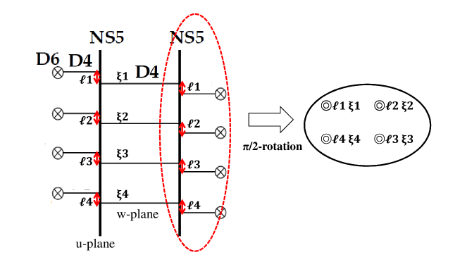
Fig. 1: Main idea: $SU(N)/SU(2)^{N-3}$ correspondence
LHS: M-theory curve of $SU(4)$ $N_{f}=8$ Yang-Mills theory embedded in $\bf{C}\times\bf{C}^{\ast}$ parameterized by $(u,w)$ $(w=\exp(-s/R),~{}R=\ell_{s}g_{s}:~{}\text{M-circle~{}radius})$; RHS: spin-chain variables $(\xi_{n},\ell_{n})$ labeling (coordinate, weight) of each puncture on ${\bf{CP}}^{1}$ (but indicating each flavor D6-brane location along $u$-plane of LHS)

AGT claimed that correlators of primary states in Liouville field theory (LFT) can get re-expressed in terms of Nekrasov’s partition function $Z_{\text{Nek}}$ of 4D ${\cal N}=2$ quiver-type $SU(2)$ superconformal field theories (SCFTs). In particular, every Riemann surface $C_{g,n}$ (whose doubly-sheeted cover is called Gaiotto curve [12]) on which LFT dwells is responsible for one specific SCFT called ${\cal T}_{g,n}(A_{1})$ such that the following equality

$$\text{conformal~{}block~{}w.r.t.~{}}C_{g,n}=\text{instanton~{}part~{}of}~{}Z_{\text{Nek}}\Big{(}{\cal T}_{g,n}(A_{1})\Big{)}$$

holds. Because of $\epsilon_{1}:\epsilon_{2}=b^{-1}:b$ [11] the one-parameter version ($\epsilon_{2}=0$) of AGT conjecture directly leads to the semiclassical LFT as $b\to 0$. Quote further the geometric Langlands correspondence [13] which associates Gaudin integrable models on the projective line with LFT at $b\to 0$. It is then plausible to put both proposals of NS and AGT into one unified scheme.

In this letter, we add a new element into the above 2D/4D correspondence. Starting from Baxter’s T-Q equation of XXX spin-chain models we found a novel interpretation of it. That is, under the semiclassical limit it possesses two aspects simultaneously. It describes
$\bullet$ 4D ${\cal N}=2$ $SU(N_{c})$ Yang-Mills with $N_{f}=2N_{c}$ flavors, ${\cal T}_{0,4}(A_{N_{c}-1})$, on the one hand and
$\bullet$ $SU(2)^{N_{c}-3}$ ($N_{c}>3$) quiver-type Yang-Mills with $N_{c}$ (four fundamental and $N_{c}-4$ bi-fundamental) hyper-multiplets, ${\cal T}_{0,N_{c}}(A_{1})$, on the other hand.
It is helpful to have a rough idea through Fig. 1. Pictorially, $C_{0,4}$ for ${\cal T}_{0,4}(A_{1})$ in RHS results from the encircled part in LHS after a $\pi/2$-rotation.

	0, 1, 2, 3	$u=x^{4}+ix^{5}$	6	7, 8, 9
D6	$\circ$	-	-	$\circ$
NS5	$\circ$	$\circ$	-	-
D4	$\circ$	-	$\circ$	-

Table 1: Type IIA D6-NS5-D4 brane configuration

In other words, the conventional Type IIA Seiberg-Witten (SW) curve (see Table 1) in fact contains another important piece of information while seen from $(u,v)$-space ($u=x^{4}+ix^{5},v=x^{7}+ix^{8}$). Here, “$\pi/2$-rotation” just means that SW differentials of two theories thus yielded are connected by exchanging $(u,s=x^{6}+ix^{10})$.

This quite unexpected phenomenon will be explained later by combining a couple of topics, say, Bethe Ansatz, Gaudin model and Liouville theory. Roughly speaking, the spin-chain variable $\ell$ $(\xi)$, highest weight (shifting parameter), is responsible for $m$ $(q)$ of RHS in Fig. 1. As summarized in Table 2, $N_{c}$ Coulomb moduli $\xi\in\bf{C}$ (one overall $U(1)$ factor) are mapped to $N_{c}-3$ gauge coupling constants $q=\exp(2\pi i\tau)\in\bf{C}^{\ast}$ where three of them are fixed to $(0,1,\infty)$ on $\bf{C}^{\ast}$. Those entries marked by $\odot$ do not have direct comparable counterparts.

$\#$ of UV parameter	LHS	RHS
Coulomb moduli	$N_{c}-1~{}({\xi})$	$\odot N_{c}-3$ ($a$)
bare flavor mass	$N_{c}~{}({\xi\pm\ell})$	$N_{c}~{}({m})$
gauge coupling	$\odot$1 $\exp(\dfrac{\Delta x^{6}+i\Delta x^{10}}{R})$	$N_{c}-3~{}(q)$

Table 2: UV parameters of two ${\cal N}=2$ theories ($N_{c}>3$) in Fig. 1

We organize this letter as follows. Sec. 2 is devoted to a further study of Fig. 2 on which our main idea Fig. 1 is based. Then Sec. 3 unifies three elements: Gaudin model, LFT and matrix model as shown in Fig. 3. Finally, in Sec. 4 we complete our proposal by examining $\lambda_{SW}$ (SW differential) and shortly discuss XYZ Gaudin models.

2 XXX spin chain

Baxter’s T-Q equation [15, 16] plays an underlying role in various spin-chain models. On the other hand, it has long been known that the low-energy Coulomb sectors of ${\cal N}=2$ gauge theories are intimately related to a variety of integrable systems [17, 18, 19, 20, 21, 22, 23]. Here, by integrable model (or solvable model) we mean that there exists some spectral curve which gives enough integrals of motion (or conserved charges). In the case of ${\cal N}=2$ $SU(N_{c})$ Yang-Mills theory with $N_{f}$ fundamental hyper-multiplets, its SW curve [24, 25] is identified with the spectral curve of an inhomogeneous periodic Heisenberg XXX spin chain on $N_{c}$ sites:

$$w+\frac{1}{w}=\frac{P_{N_{c}}(u)}{\sqrt{Q_{N_{f}}(u)}}.$$ (2.1)

Here, two polynomials $P_{N_{c}}$ and $Q_{N_{f}}$ encode respectively parameters of ${\cal N}=2$ vector- and hyper-multiplets. Meanwhile, the meromorphic SW differential $\lambda_{SW}=ud\log w$ provides a set of “special coordinates” through its period integrals (see Table 2):

$$\xi_{n}=\oint_{\alpha_{n}}\lambda_{SW},~{}~{}~{}~{}~{}~{}\frac{\partial{\cal F}_{SW}}{\partial\xi_{n}}=\xi^{D}_{n}=\oint_{\beta_{n}}\lambda_{SW},~{}~{}~{}~{}~{}~{}\xi_{n}\pm\ell_{n}=\oint_{\gamma_{n}^{\pm}}\lambda_{SW}$$ (2.2)

where ${\cal F}_{SW}$ is the physical prepotential.

2.1 Baxter’s T-Q equation

Indeed, (2.1) arises from (up to $w\to\sqrt{Q_{N_{f}}}w$)

$$\det\big{(}w-{T}(u)\big{)}=0~{}~{}\to~{}~{}w^{2}-\mathop{\rm tr}T(u)w+\det T(u)=0,~{}~{}~{}~{}~{}~{}T(u):~{}2\times 2\text{~{}monodromy~{}matrix},$$

$$\det T(u)=Q_{N_{f}}(u)=\prod_{n=1}^{N_{c}}(u-m^{-}_{n})(u-m^{+}_{n}),~{}~{}~{}~{}~{}~{}m^{\pm}_{n}=\xi_{n}\pm\ell_{n}.$$

$\mathop{\rm tr}T(u)=t(u)=P_{N_{c}}(u)=\langle\det(u-\Phi)\rangle$, transfer matrix, encodes the quantum vev of the adjoint scalar field $\Phi$. In fact, (2.1) belongs to the $conformal$ case where $N_{f}=2N_{c}$ bare flavor masses are indicated by $m_{n}^{\pm}$. It is time to quote Baxter’s T-Q equation:

$$t(u)Q(u)=\triangle_{+}(u)Q(u-2\eta)+\triangle_{-}(u)Q(u+2\eta).$$ (2.3)

Some comments follow:
$\bullet$ $\eta$ is Planck-like and ultimately gets identified with $\epsilon_{1}$ (one of two $\Omega$-background parameters) in Sec. 4.
$\bullet$ As a matter of fact, (2.3) boils down to (2.1) (up to $w\to\sqrt{Q_{N_{f}}}w$) as $\eta\to 0$. Curiously, then its $\lambda_{SW}$ signals the existence of another advertised ${\cal N}=2$ theory. The situation is pictorially shown in Fig. 1.
$\bullet$ Remark again that SW differentials of two theories are connected by exchanging two holomorphic coordinates $(u,s)$ but their M-lifted [26] Type IIA brane configurations are not. Instead, the $\pi/2$-rotated part is closely related to ${\cal N}=2$ Gaiotto’s curve. A family of quiver-type $SU(2)$ SCFTs ${\cal T}_{0,n}(A_{1})$ discovered by Gaiotto [12] is hence made contact with.

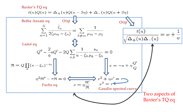
Fig. 2: Mathematical description of Fig. 1
Up to ${\cal O}(\eta)$, Baxter’s T-Q equation and Bethe Ansatz equations of it describe two kinds of ${\cal N}=2$ gauge theories which however are related by one $\lambda_{SW}$

2.2 More detail

Let us refine the above argument. Consider a quantum spin-chain built over an $N$-fold tensor product ${\cal H}=\otimes_{n=1}^{N}V_{n}$. In other words, at each site labeled by $n$ we assign an irreducible representation $V_{n}$ of ${\mathfrak{sl}}_{2}$ which is $(\ell_{n}+1)$-dimensional where $\ell_{n}=0,1,2,\cdots$. Therefore, $\ell_{n}$ denotes the highest weight. Within the context of QISM, monodromy and transfer matrices are defined respectively by

$$T(u)=\left(\begin{array}[]{cc}A_{N}(u)&B_{N}(u)\\ C_{N}(u)&D_{N}(u)\end{array}\right)=L_{N}(u-\xi_{N})\cdots L_{1}(u-\xi_{1}),$$ (2.6)

$$\widehat{t}(u)=A_{N}(u)+D_{N}(u).$$

$V_{n}$ is acted on by the $n$-th Lax operator $L_{n}$. By $inhomogeneous$ one means that the spectral parameter $u$ has been shifted by $\xi$. Conventionally, $\widehat{t}(u)$ or its eigenvalue $t(u)$ is called generating function because a series of conserved charges can be extracted from its coefficients owing to $[\widehat{t}(u),\widehat{t}(v)]=0$. The commutativity arises just from the celebrated Yang-Baxter equation.

As far as the inhomogeneous periodic XXX spin chain is concerned, its T-Q equation reads ($\ell=\eta\widetilde{\ell}$)

$$t(u)Q(u)=\triangle_{+}(u)Q(u-2\eta)+\triangle_{-}(u)Q(u+2\eta),$$

$$Q(u)=\prod_{k=1}^{K}(u-\mu_{k}),~{}~{}~{}~{}~{}~{}\triangle_{\pm}=\prod_{n=1}^{N}{(u-\xi_{n}\pm\eta\widetilde{\ell}_{n})}$$ (2.7)

where each Bethe root $\mu_{k}$ satisfies a set of Bethe Ansatz equations:

$$\frac{\triangle_{+}(\mu_{k})}{\triangle_{-}(\mu_{k})}=\prod_{n=1}^{N}\frac{{(\mu_{k}-\xi_{n}+\eta\widetilde{\ell}_{n})}}{{(\mu_{k}-\xi_{n}-\eta\widetilde{\ell}_{n})}}=\prod_{l(\neq k)}^{K}\frac{\mu_{k}-\mu_{l}+2\eta}{\mu_{k}-\mu_{l}-2\eta}.$$ (2.8)

A semiclassical limit is facilitated by the $\eta$ dependence. Through

$$\frac{t(u)}{\sqrt{\triangle_{+}\triangle_{-}}}=\frac{Q(u-2\eta)}{Q(u)}\sqrt{\frac{\triangle_{+}}{\triangle_{-}}}+\frac{Q(u+2\eta)}{Q(u)}\sqrt{\frac{\triangle_{-}}{\triangle_{+}}}$$ (2.9)

and omitting ${\cal O}(\eta^{2})$, we have

$$\frac{t(u)}{\sqrt{\triangle_{+}(u)\triangle_{-}(u)}}=w+\frac{1}{w},~{}~{}~{}~{}~{}~{}~{}~{}~{}w\equiv\sqrt{\frac{\triangle_{+}}{\triangle_{-}}}(1-2\eta\frac{Q^{\prime}}{Q})$$ (2.10)

which exactly reduce to (2.1). Throughout this letter, ($\eta,\widetilde{\ell}$) while kept finite are, respectively, small and large.

From now on, we call $\lambda_{SW}=ud\log w\equiv\lambda_{SW}^{\eta}$ “$\eta$-deformed” SW differential as in [28, 29]:

$$\lambda_{SW}^{\eta}=2\eta ud\left(\frac{\Psi^{\prime}}{\Psi}\right)+{\cal O}(\eta^{2}),~{}~{}~{}~{}~{}~{}~{}~{}~{}\Psi=\frac{1}{Q(u)}\prod_{n}(u-\xi_{n})^{\widetilde{\ell}_{n}/2}.$$ (2.11)

Also, up to ${\cal O}(\eta)$ (2.8) reads

$$\sum_{n=1}^{N}\frac{\widetilde{\ell}_{n}}{2(\mu_{k}-\xi_{n})}=\sum^{K}_{l(\neq k)}\frac{1}{(\mu_{k}-\mu_{l})}.$$ (2.12)

That $\lambda^{\eta}_{SW}$ looks strikingly similar to (2.12) signals the existence of RHS in Fig. 1. Fig. 2 outlines our logic. One will find that $\lambda_{SW}^{\eta}$ naturally emerges as the holomorphic one-form of Gaudin’s spectral curve which captures Gaiotto’s curve for ${\cal T}_{0,N}(A_{1})$. In what follows, our goal is to show that $\lambda_{SW}^{\eta}$ does reproduce the $\epsilon_{1}$-deformed SW prepotential w.r.t. ${\cal T}_{0,N}(A_{1})$.

Several comments follow:
$\bullet$ In M-theory D6-branes correspond to singular loci of $XY={{\triangle_{+}(u)\triangle_{-}(u)}}$. This simply means that one incorporates flavors via replacing a flat ${\mathbf{R}}^{4}$ over $(u,s)$ by a resolved ${\bf A}_{2N_{c}-1}$-type singularity.
$\bullet$ Without flavors (i.e. turning off $\ell$) $\int\lambda_{SW}^{\eta}$ looks like a logarithm of the usual Vandermonde. This happens in the familiar Dijkgraaf-Vafa story [30, 31, 32] without any tree-level potential which brings ${\cal N}=2$ pure Yang-Mills to ${\cal N}=1$ descendants.
$\bullet$ Surely, this intuition is noteworthy in view of (2.12) which manifests itself as the saddle-point condition within the context of matrix models. To pursue this interpretation, one should regard $\mu$’s as diagonal elements of ${\cal M}$ (Hermitian matrix of size $K\times K$). Besides, the tree-level potential now obeys

$${\cal W}^{\prime}(x)=-\sum_{n=1}^{N}\frac{\ell_{n}}{(x-\xi_{n})}.$$

In other words, we are equivalently dealing with “${\cal N}=2$” Penner-type matrix models which have been heavily investigated recently in connection with AGT conjecture due to [33]. We will return to these points soon.

3 XXX Gaudin model

Momentarily, we focus on another well-studied integrable model: XXX Gaudin model. The essential difference between Heisenberg and Gaudin models amounts to the definition of their generating functions. Following Fig. 3 we want to explain two important aspects of Gaudin’s spectral curve.

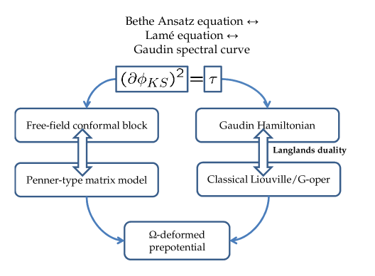
Fig. 3: Flow chart of Sec. 3

3.1 RHS of Fig. 3

Expanding around small $\eta$, we yield

$$L_{n}(u)=1+2\eta{\cal L}_{n}+O(\eta^{2}),$$ (3.1)

$$T(u)=1+2\eta{\cal T}+\eta^{2}{\cal T}^{(2)}+O(\eta^{3}),$$ (3.2)

$$t(u)=1+\eta^{2}{\text{tr}}{\cal T}^{(2)}+O(\eta^{3}),$$ (3.3)

$$\tau(u)\equiv\frac{1}{2}\eta^{2}{\text{t}r}{\cal T}^{2},~{}~{}~{}~{}~{}~{}~{}~{}~{}~{}{\cal T}=\sum_{n}{\cal L}_{n}=\left(\begin{array}[]{cc}A(u)&B(u)\displaystyle\\ C(u)&-A(u)\displaystyle\end{array}\right)$$ (3.6)

where

$$A(u)=\displaystyle\sum_{n=1}^{N}\frac{J_{n}^{z}}{u-\xi_{n}},~{}~{}~{}~{}~{}~{}~{}~{}~{}B(u)=\sum_{n=1}^{N}\frac{J_{n}^{-}}{u-\xi_{n}},~{}~{}~{}~{}~{}~{}~{}~{}~{}C(u)=\sum_{n=1}^{N}\frac{J_{n}^{+}}{u-\xi_{n}}$$ (3.7)

while $\vec{J}=(J^{z},J^{\pm})$ represents generators of ${\mathfrak{sl}}_{2}$ Lie algebra. Instead of $\mathop{\rm tr}{\cal T}^{(2)}$ ($\mathop{\rm tr}{\cal T}=0$) the generating function adopted is ($s=\widetilde{\ell}/2=\ell/2\eta$)

$$\tau(u)=\sum_{n=1}^{N}\Big{\{}\frac{\eta^{2}s_{n}(s_{n}+1)}{(u-\xi_{n})^{2}}+\frac{c_{n}}{u-\xi_{n}}\Big{\}},~{}~{}~{}~{}~{}~{}~{}~{}~{}c_{n}=\sum_{i\neq n}^{N}\frac{2\eta^{2}\vec{J}_{n}\cdot\vec{J}_{i}}{\xi_{n}-\xi_{i}},~{}~{}~{}~{}~{}~{}~{}~{}~{}\vec{J}_{n}\cdot\vec{J}_{n}=s_{n}(s_{n}+1).$$ (3.8)

Conventionally, $c_{n}$’s are called Gaudin Hamiltonians which commute with one another as a result of the classical Yang-Baxter equation.

$$\Sigma:~{}x^{2}=\tau(u)\subset{T^{\ast}C}$$

is the $N$-site Gaudin spectral curve, a doubly-sheeted cover of $C\equiv{\bf{CP}}^{1}\backslash\{\xi_{1},\cdots,\xi_{N}\}$.

According to the geometric Langlands correspondence, $c_{n}$’s give exactly $accessory$ parameters of a $G$-oper:

$${\cal D}=-\displaystyle\partial_{z}^{2}+\sum_{n=1}^{N}\frac{\delta_{n}}{(z-\xi_{n})^{2}}+\sum_{n=1}^{N}\frac{\widetilde{c}_{n}}{z-\xi_{n}},~{}~{}~{}~{}~{}~{}~{}~{}~{}\delta=s(s+1),~{}~{}~{}~{}~{}~{}~{}~{}~{}c=\eta^{2}\widetilde{c}$$

defined over $C={\bf{CP}}^{1}\backslash\{\xi_{1},\cdots,\xi_{N}\}$. The non-singular behavior of ${\cal D}$ is ensured by imposing

$$\sum_{n=1}^{N}{\widetilde{c}}_{n}=0,~{}~{}~{}~{}~{}~{}~{}~{}~{}\sum_{n=1}^{N}(\xi_{n}\widetilde{c}_{n}+\delta_{n})=0,~{}~{}~{}~{}~{}~{}~{}~{}~{}\sum_{n=1}^{N}(\xi_{n}^{2}\widetilde{c}_{n}+2\xi_{n}\delta_{n})=0.$$

Certainly, one soon realizes that $\tau(u)$ here is nothing but the holomorphic LFT (2,0) stress-tensor as the central charge $1+6Q^{2}$ goes to infinity (or $b\to 0$). Namely,

$$\eta^{-2}\tau\equiv\frac{1}{2}\partial_{z}^{2}\varphi_{cl}-\frac{1}{4}(\partial_{z}\varphi_{cl})^{2}=\sum_{n=1}^{N}\frac{\delta_{n}}{(z-\xi_{n})^{2}}+\sum_{n=1}^{N}\frac{\widetilde{c}_{n}}{z-\xi_{n}}.$$

In terms of LFT, the second equality comes from Ward identity of the stress-tensor $T_{L}=\frac{1}{2}Q\partial_{z}^{2}\phi-\frac{1}{4}(\partial_{z}\phi)^{2}$ inserted in $\langle\prod_{n}V_{\alpha_{n}}\rangle$ subject to $b\to 0$. Here, $V_{\alpha}=\exp({2}\alpha\phi)$ denotes the primary field $(\Delta_{\alpha}=\alpha(Q-\alpha),~{}Q=b+{b}^{-1})$. As $b\to 0$,

$$\big{\langle}(-T_{L})\prod_{n}V_{\alpha_{n}}\big{\rangle}=\int{\cal D}\phi\exp(-{\bf S}_{\text{tot}})(-T_{L})~{}\to~{}\exp(-\dfrac{1}{b^{2}}{\cal S}_{\text{tot}}[\varphi_{cl}])\dfrac{1}{\eta^{2}b^{2}}\tau$$

such that for the unique saddle-point to ${\cal S}_{\text{tot}}[\varphi]$ one has (Polyakov conjecture)

$$\widetilde{c}_{n}=\frac{\partial{\cal S}_{\text{tot}}[\varphi_{cl}]}{\partial\xi_{n}},~{}~{}~{}~{}~{}~{}~{}~{}~{}|\widetilde{\alpha}_{n}|=b|\alpha_{n}|=s_{n}$$ (3.9)

where on a large disk $\Gamma$

$${\bf S}_{\text{tot}}=\int_{\Gamma}d^{2}z\Big{(}\frac{1}{4\pi}|\partial_{z}\phi|^{2}+{\mu}e^{{2}b\phi}\Big{)}+\text{boundary~{}terms},~{}~{}~{}~{}~{}~{}~{}~{}~{}{\bf S}_{\text{tot}}[\phi]=\dfrac{1}{b^{2}}{\cal S}_{\text{tot}}[\varphi].$$

Note that $\varphi_{cl}$ satisfies Liouville’s equation and is important during uniformizing Riemann surfaces with constant negative curvature. Usually, $\widetilde{\alpha}=b\alpha$ is kept fixed during $b\to 0$. It is necessary that $\eta=\hbar/b$ due to $b|\alpha|=\ell/2\eta$. This confirms in advance $\eta=\epsilon_{1}$ due to AGT dictionary.

3.2 LHS of Fig. 3

As shown in [37], $\tau(u)$ has another form in terms of the eigenvalue $a(u)$ of $A(u)$:

$$\tau(u)=a^{2}-\eta a^{\prime}-2\eta\sum_{k}\frac{a(u)-a(\mu_{k})}{u-\mu_{k}},~{}~{}~{}~{}~{}~{}~{}~{}~{}a(u)\equiv\sum_{n=1}^{N}\frac{\eta s_{n}}{(u-\xi_{n})}$$ (3.10)

with $\mu_{k}$’s being Bethe roots. This expression is extremely illuminating in connection with Penner-type matrix models. Borrowing $Q(u)$ from (2.7) and defining

$$\Re(u)\equiv Q(u)\exp\Big{(}-\frac{1}{\eta}\int^{u}a(y)dy\Big{)}=\prod_{k}(u-\mu_{k})\prod_{n}(u-\xi_{n})^{-s_{n}},$$ (3.11)

we can verify that there holds

$$\eta x^{\prime}+x^{2}=\tau,~{}~{}~{}~{}~{}~{}~{}~{}~{}x(u)=\eta\frac{\Re^{\prime}(u)}{\Re(u)}=-a+\sum_{k}\frac{\eta}{u-\mu_{k}}.$$ (3.12)

This is the so-called Lamé equation in disguise. Equivalently, $\Re(u)$ solves a Fuchs-type equation $\big{(}\eta^{2}\partial_{u}^{2}-\tau(u)\big{)}\Re(u)=0$ with $N$ regular singularities on ${\bf{CP}}^{1}$.

Compared with $x^{2}$, $\eta x^{\prime}$ becomes subleading. Further getting rid of $\eta x^{\prime}$, we arrive at Gaudin’s spectral curve

$$x^{2}=\tau.$$ (3.13)

In view of (3.12), it is tempting to introduce $\phi_{KS}$, i.e. Kodaira-Spencer field w.r.t. $Z^{M}$ defined in (3.16). That is,

$$2x\equiv\partial\phi_{KS}={\cal W}^{\prime}+2\eta\mathop{\rm tr}\Big{\langle}\frac{1}{u-{\cal M}}\Big{\rangle}_{Z^{M}}.$$ (3.14)

Subsequently, (3.13) becomes precisely the spectral curve of $Z^{M}$. Remark that

$$\oint\partial\phi_{KS}du=-\oint\lambda^{\eta}_{SW}$$ (3.15)

up to a total derivative term. Additionally, it is well-known that from the period integral (3.15) one yields the tree-level free energy ${\cal F}_{0}$ of $Z^{M}$:

$$Z^{M}=\int_{K\times K}{\cal{DM}}\exp\left[{\frac{1}{\eta}\cal{W(M)}}\right],~{}~{}~{}~{}~{}~{}~{}~{}~{}{\cal W}^{\prime}=-\sum_{n=1}^{N}\frac{\ell_{n}}{(u-\xi_{n})},~{}~{}~{}~{}~{}~{}~{}~{}~{}K\eta=\text{fixed}.$$ (3.16)

Of course, the saddle-point of $Z^{M}$ is dictated by (2.12). We want to display in Sec. 4 that ${\cal F}_{0}$ is surely related to ${\cal T}_{0,N}(A_{1})$. In view of (3.15), we refer to this as the advertised $SU(N)/SU(2)^{N-3}$ $(N>3)$ correspondence.

For Gaudin’s spectral curve, due to $(x,u)\in\bf{C}\times\bf{C}^{\ast}$ we introduce $v=xu$ such that $xdu$ here and the former $ud\log w$ of ${\cal T}_{0,4}(A_{N-1})$ look more symmetrical. Moreover, the $\pi/2$-rotation noted in Fig. 1 is only pictorial otherwise one naively has $SU(N)/SU(2)^{N-1}$ correspondence instead.

3.2.1 Free-field representation

As another crucial step, we rewrite $Z^{M}$ in terms of a multi-integral over diagonal elements of ${\cal M}$:

$$Z^{M}\equiv\oint dz_{1}\cdots\oint dz_{K}\prod_{i<j}(z_{i}-z_{j})^{2}\prod_{i,n}(z_{i}-\xi_{n})^{-\widetilde{\ell}_{n}}\prod_{n<m}(\xi_{n}-\xi_{m})^{{\widetilde{\ell}_{n}\widetilde{\ell}_{m}}/2}.$$ (3.17)

A constant term involving only $\xi$’s is multiplied by hand. This form then realizes a chiral conformal block of $N$ LFT primary fields via Feigin-Fuchs free-field representation. Notably, the charge balance condition is respected in the presence of background charge $Q$ via inserting $K$ screening operators $\oint dz\exp{2}{b^{-1}}\phi(z)$ of zero conformal weight. Also, the free propagator $\big{\langle}\phi(z_{1})\phi(z_{2})\big{\rangle}_{\text{free}}=-\log(z_{1}-z_{2})^{1/2}$ is used.

Assume the genus expansion $Z^{M}=\exp(\eta^{-2}{\cal F}_{0}+\cdots)$ and

$$\lim_{b\to 0}\log\Big{\langle}V_{-\widetilde{\ell}_{1}/2b}(\xi_{1})\cdots V_{-\widetilde{\ell}_{N}/2b}(\xi_{N})\Big{\rangle}_{\text{conformal~{}block}}=-b^{-2}\widetilde{F}.$$

$\widetilde{F}$ named $classical$ conformal block appeared in the pioneering work of Zamolodchikov and Zamolodchikov [38]. Based on the above discussion, one can anticipate that $\eta^{2}\widetilde{F}={\cal F}_{0}$. Next, to identify ${\cal F}_{0}$ with the $\Omega$-deformed SW prepotential for ${\cal T}_{0,N}(A_{1})$ serves as the last step towards completing our proposal.

4 Application and discussion

Without loss of generality, we examine a concrete example: $N=4$. As a result, ${\cal F}_{0}$ generated by the period integral of $\lambda^{\eta}_{SW}=-\partial\phi_{KS}du$ is indeed the very $\epsilon_{1}$-deformed SW prepotential of ${\cal T}_{0,4}(A_{1})$. Quote the known $\tau(u)$ for $N=4$ from [38]:

$$\eta^{-2}\tau(u)=\frac{\delta_{1}}{u^{2}}+\frac{\delta_{2}}{(u-q)^{2}}+\frac{\delta_{3}}{(1-u)^{2}}+\frac{\delta_{1}+\delta_{2}+\delta_{3}-\delta_{4}}{u(1-u)}+\frac{q(1-q)\widetilde{c}(q)}{u(u-q)(1-u)}.$$ (4.1)

Via projective invariance $q$ represents the cross-ratio of four marked points $(\xi_{1},\xi_{2},\xi_{3},\xi_{4})\equiv(0,1,q,\infty)$ on ${\bf{CP}}^{1}$.

The residue of $\tau$ around $u=1$ is ($v=xu$)

$$q\widetilde{c}(q)=-\eta^{-2}\oint ux^{2}du=-\frac{1}{2}\eta^{-2}\oint v\lambda_{SW}^{\eta}=q\frac{\partial}{\partial{q}}{\widetilde{F}}_{\delta,\delta_{n}}(q),~{}~{}~{}~{}~{}~{}~{}~{}~{}(n=1,\cdots,4),$$ (4.2)

$$\widetilde{F}_{\delta,\delta_{n}}(q)=(\delta-\delta_{1}-\delta_{2})\log q+\frac{(\delta+\delta_{1}-\delta_{2})(\delta+\delta_{3}-\delta_{4})}{2\delta}q+{\cal O}(q^{2})$$

where Polyakov’s conjecture (3.9) is applied in the last equality of (4.2). Notice that only the holomorphic $\widetilde{F}$ in ${\cal S}_{\text{tot}}$ survives ${\partial}/{\partial}q$. Conversely, by taking into account the stress-tensor nature of the spectral curve $(\partial\phi_{KS})^{2}=4\tau$ in Hermitian matrix models, $\widetilde{F}$ can be replaced by ${\cal F}_{0}$ as a result of Virasoro algebra. This observation supports the above $\eta^{2}\widetilde{F}={\cal F}_{0}$.

Finally, we need another ingredient: Matone’s relation [39, 40, 41]. As is proposed in [42, 28, 29], the $\epsilon_{1}$-deformed version is

$$\langle\mathop{\rm tr}\Phi^{2}\rangle_{\epsilon_{1}}=2\bar{q}\partial_{\bar{q}}{W},~{}~{}~{}~{}~{}~{}~{}~{}~{}\bar{q}=\exp(2\pi i\bar{\tau}_{UV})$$ (4.3)

for, say, ${\cal N}=2$ ${\cal T}_{0,4}(A_{1})$ theory where

$$\frac{1}{\epsilon_{1}\epsilon_{2}}{W(\epsilon_{1})}\equiv\lim_{\epsilon_{2}\to 0}\log Z_{\text{Nek}}\big{(}a,\vec{m},\bar{q},\epsilon_{1},\epsilon_{2}\big{)},~{}~{}~{}~{}~{}$$

$${a}:~{}\text{UV~{}vev~{}of~{}}\Phi,~{}~{}~{}~{}~{}~{}~{}~{}~{}\vec{m}:~{}\text{four~{}bare~{}flavor~{}masses}.$$

Now, (4.2) and (4.3) together manifest $\lambda^{\eta}_{SW}$ as the $\epsilon_{1}$-deformed SW differential for ${\cal T}_{0,4}(A_{1})$ if there holds

$$\frac{1}{b^{2}}{\widetilde{F}}_{\delta,\delta_{n}}(q)=\frac{1}{\hbar^{2}}{\cal F}_{0}=\lim_{\epsilon_{2}\to 0}\frac{1}{\epsilon_{1}\epsilon_{2}}{W(\epsilon_{1})}$$ (4.4)

under $q=\bar{q}$, $\epsilon_{1}=\eta$ and $\epsilon_{1}{\epsilon_{2}}=\hbar^{2}$. In fact, (4.4) has already been verified in [43].

Theory of RHS in Fig. 1 ($N=4$)
$q=\dfrac{(\xi_{1}-\xi_{3})(\xi_{2}-\xi_{4})}{(\xi_{2}-\xi_{3})(\xi_{1}-\xi_{4})}$
$\epsilon_{1}{m}\leftrightarrow\widetilde{\ell}$
$(\epsilon_{1},\epsilon_{2})=(\eta,0)$
$a=\oint_{\alpha}\lambda^{\eta}_{SW}$
$\epsilon_{1}^{2}\dfrac{\partial\widetilde{F}}{\partial a}=\oint_{\beta}\lambda^{\eta}_{SW}$

Table 3: Quantities of RHS in Fig. 1 in terms of spin-chain variables

To conclude, by examining $\lambda^{\eta}_{SW}$ we have found that Baxter’s T-Q equation encodes simultaneously two kinds of ${\cal N}=2$ theories, ${\cal T}_{0,N}(A_{1})$ and ${\cal T}_{0,4}(A_{N-1})$. We call this remarkable property $SU(N)/SU(2)^{N-3}$ correspondence.

4.1 Discussion

$\bullet$ Based on (2.10) and (2.11), we have at the level of $\lambda^{\eta}_{SW}$

$$\log w=2\eta\frac{\Psi^{\prime}}{\Psi},~{}~{}~{}~{}~{}~{}~{}~{}~{}w=\frac{A+\sqrt{A^{2}-4}}{2},~{}~{}~{}~{}~{}~{}~{}~{}~{}A=\frac{P_{N_{c}}}{\sqrt{Q_{N_{f}}}}.$$ (4.5)

Namely, all quantum $SU(N_{c})$ Coulomb moduli encoded inside $P_{N_{c}}(u)\equiv\langle\det(u-\Phi)\rangle$ are determined by using spin-chain variables $(\eta,\xi,\ell)$. This fact is consistent with (2.2).
$\bullet$ Besides, from Table 3 we find that the transformation between ${\cal F}_{SW}$ in (2.2) and $\widetilde{F}$ is quite complicated. Although sharing the same SW differential (up to a total derivative term), two theories have diverse IR dynamics because both of their gauge group and matter content differ. To pursue a concrete interpolation between them is under investigation.

4.2 XYZ Gaudin model

There are still two other Gaudin models, say, trigonometric and elliptic ones. Let us briefly discuss the elliptic type because it sheds light on ${\cal N}=2$ ${\cal T}_{1,n}(A_{1})$ theory. Now, Bethe roots satisfy the following classical Bethe Ansatz equation:

$$\sum_{n=1}^{N}\frac{s_{n}\theta_{11}^{\prime}(\mu_{k}-\xi_{n})}{\theta_{11}(\mu_{k}-\xi_{n})}=-\pi i\nu+\sum_{l(\neq k)}\frac{\theta_{11}^{\prime}(\mu_{k}-\mu_{l})}{\theta_{11}(\mu_{k}-\mu_{l})},~{}~{}~{}~{}~{}~{}~{}~{}~{}\nu\in\text{integer}.$$ (4.6)

Regarding it as a saddle-point condition, we are led to the spectral curve analogous to (3.13)

$$\begin{split}x^{2}&=\left[\displaystyle\sum_{n=1}^{N}\frac{s_{n}\theta_{11}^{\prime}(u-\xi_{n})}{\theta_{11}(u-\xi_{n})}-\sum^{K}_{k=1}\frac{\theta_{11}^{\prime}(u-\mu_{k})}{\theta_{11}(u-\mu_{k})}\right]^{2}\\ &=\sum_{n=1}^{N}s_{n}(s_{n}+1)\wp(u-\xi_{n})+\sum_{n=1}^{N}H_{n}\zeta(u-\xi_{n})+H_{0}\end{split}$$

where

$$\begin{split}H_{n}&=\sum^{N}_{i\neq n}\sum_{a=1}^{3}w_{a}(\xi_{n}-\xi_{i})J_{n}^{a}J_{i}^{a},\\ H_{0}&=\sum_{n=1}^{N}\sum_{a=1}^{3}\Bigl{\{}-\wp\left(\frac{\omega_{5-a}}{2}\right)J_{n}^{a}J_{n}^{a}+\sum_{i\neq n}w_{a}(\xi_{i}-\xi_{n})\left[\zeta\Bigl{(}\xi_{n}-\xi_{i}+\frac{\omega_{5-a}}{2}\Bigr{)}-\zeta\Bigl{(}\frac{\omega_{5-a}}{2}\Bigr{)}\right]J_{n}^{a}J_{i}^{a}\Bigr{\}}.\end{split}$$ (4.7)

Here, $\wp(u)$ and $\zeta(u)$ respectively denote Weierstrass $\wp$- and $\zeta$-function. Periods of $\wp(u)$ are (see Appendix A for $w_{a}$)

$$\begin{split}\omega_{1}=\omega_{4}=1,~{}~{}~{}~{}~{}~{}~{}~{}~{}\omega_{2}=\tau,~{}~{}~{}~{}~{}~{}~{}~{}~{}\omega_{3}=\tau+1.\end{split}$$ (4.8)

Notice that $H_{n}$’s ($\sum H_{n}=0$) are known as elliptic Gaudin Hamiltonians [44, 45]. All these are elliptic counterparts of those in the rational XXX model. According to the logic of Fig. 3, it will be interesting to verify whether the XYZ one-form $xdu$ reproduces the $\epsilon_{1}$-deformed ${\cal N}=2^{\ast}$ SW prepotential when $n=1$

Appendix A Definition of $w_{n}$

In Appendix A, $w_{n}$ that appears in (4.7) will be defined according to [44, 45]. We choose periods of $\wp(u)$ as in (4.8). Weierstrass $\sigma$-function is as follows:

$$\begin{split}\sigma(u)&=\sigma(u;\omega_{1},\omega_{2})\\ &=u\prod_{\begin{subarray}{c}(n,m)\neq(0,0)\\ n,m\in\bf{Z}\end{subarray}}\left(1-\frac{u}{n\omega_{1}+m\omega_{2}}\right)\exp\left[\frac{u}{n\omega_{1}+m\omega_{2}}+\frac{1}{2}\left(\frac{u}{n\omega_{1}+m\omega_{2}}\right)^{2}\right].\end{split}$$ (A.1)

Note that $\sigma(u)$ satisfies

$$\begin{split}\zeta(u)=\frac{\sigma^{\prime}(u)}{\sigma(u)},~{}~{}~{}~{}~{}~{}~{}~{}~{}~{}~{}~{}\wp(u)=-\zeta^{\prime}(u).\end{split}$$ (A.2)

We introduce $(e_{a},\eta_{a},\varsigma_{a})$ which are related to $\omega_{a}$ by

$$\begin{split}e_{a}=\wp(\omega_{a}/2),~{}~{}~{}~{}~{}~{}~{}\eta_{a}=\zeta(\omega_{a}/2),~{}~{}~{}~{}~{}~{}~{}\varsigma_{a}=\sigma(\omega_{a}/2),~{}~{}~{}~{}~{}~{}a=1,2,3.\end{split}$$ (A.3)

Using them we further have

$$\begin{split}\sigma_{00}(u)&=\frac{\exp\left[-\left(\eta_{1}+\eta_{2}\right)u\right]}{\varsigma_{3}}\sigma\left(u+\frac{\omega_{3}}{2}\right),\\ \sigma_{10}(u)&=\frac{\exp\left(-\eta_{1}u\right)}{\varsigma_{1}}\sigma\left(u+\frac{\omega_{1}}{2}\right),\\ \sigma_{01}(u)&=\frac{\exp\left(-\eta_{2}u\right)}{\varsigma_{2}}\sigma\left(u+\frac{\omega_{2}}{2}\right).\end{split}$$ (A.4)

Note that Jacobi’s $\vartheta$-functions are

$$\begin{split}\vartheta_{00}(u)&=\vartheta(u;\tau)=\vartheta(u)=\sum_{n=-\infty}^{\infty}\exp\left(\pi{i}n^{2}\tau+2\pi{i}nu\right),\\ \vartheta_{01}(u)&=\vartheta\left(u+\frac{1}{2}\right),\\ \vartheta_{10}(u)&=\exp\left(\frac{1}{4}\pi{i}\tau+\pi{i}u\right)\vartheta\left(u+\frac{1}{2}\tau\right),\\ \vartheta_{11}(u)&=\exp\left(\frac{1}{4}\pi{i}\tau+\pi{i}(u+\frac{1}{2})\right)\vartheta\left(u+\frac{1}{2}+\frac{1}{2}\tau\right)\end{split}$$ (A.5)

from which Weierstrass $\sigma$-functions are defined as below:

$$\begin{split}\omega_{1}\exp\left(\frac{\eta_{1}}{\omega_{1}}u^{2}\right)\frac{\displaystyle\vartheta_{11}\left(\frac{u}{\omega_{1}}\right)}{\displaystyle\vartheta^{\prime}_{11}\left(0\right)}=\sigma(u),~{}~{}~{}~{}~{}~{}\exp\left(\frac{\eta_{1}}{\omega_{1}}u^{2}\right)\frac{\displaystyle\vartheta_{ab}\left(\frac{u}{\omega_{1}}\right)}{\displaystyle\vartheta^{\prime}_{ab}\left(0\right)}=\sigma_{ab}(u)~{}~{}~{}~{}~{}~{}(ab=0).\end{split}$$ (A.6)

Finally, $w_{a}(u)$ can be obtained as follows:

$$\begin{split}w_{1}(u)&=\frac{\mathrm{cn}(u\sqrt{e_{1}-e_{3}};\sqrt{\dfrac{e_{2}-e_{3}}{e_{1}-e_{3}}})}{\mathrm{sn}(u\sqrt{e_{1}-e_{3}};\sqrt{\dfrac{e_{2}-e_{3}}{e_{1}-e_{3}}})}=\frac{\sigma_{10}(u)}{\sigma(u)}=\frac{\vartheta^{\prime}_{11}(0)}{\vartheta_{10}(0)}\frac{\vartheta_{10}(u)}{\vartheta_{11}(u)},~{}~{}~{}~{}~{}\\ w_{2}(u)&=\frac{\mathrm{dn}(u\sqrt{e_{1}-e_{3}};\sqrt{\dfrac{e_{2}-e_{3}}{e_{1}-e_{3}}})}{\mathrm{sn}(u\sqrt{e_{1}-e_{3}};\sqrt{\dfrac{e_{2}-e_{3}}{e_{1}-e_{3}}})}=\frac{\sigma_{00}(u)}{\sigma(u)}=\frac{\vartheta^{\prime}_{11}(0)}{\vartheta_{00}(0)}\frac{\vartheta_{00}(u)}{\vartheta_{11}(u)},\\ w_{3}(u)&=\frac{1}{\mathrm{sn}(u\sqrt{e_{1}-e_{3}};\sqrt{\dfrac{e_{2}-e_{3}}{e_{1}-e_{3}}})}=\frac{\sigma_{01}(u)}{\sigma(u)}=\frac{\vartheta^{\prime}_{11}(0)}{\vartheta_{01}(0)}\frac{\vartheta_{01}(u)}{\vartheta_{11}(u)}.\end{split}$$ (A.7)

References

- [1] N. A. Nekrasov and S. L. Shatashvili, “Quantum integrability and supersymmetric vacua,” Prog. Theor. Phys. Suppl. 177 (2009) 105-119. [arXiv:0901.4748[hep-th]].
- [2] N. A. Nekrasov and S. L. Shatashvili, “Quantization of Integrable Systems and Four Dimensional Gauge Theories,” [arXiv:0908.4052[hep-th]].
- [3] N. Nekrasov, A. Rosly and S. Shatashvili, “Darboux coordinates, Yang-Yang functional, and gauge theory,” [arXiv:1103.3919 [hep-th]].
- [4] N. A. Nekrasov, “Seiberg-Witten Prepotential from Instanton Counting,” Adv. Theor. Math. Phys. 7 (2004) 831-864. [hep-th/0206161].
- [5] N. Nekrasov and A. Okounkov, “Seiberg-Witten Theory and Random Partitions,” [hep-th/0306238].
- [6] D. Orlando, S. Reffert, [arXiv:1011.6120 [hep-th]].
- [7] Y. Zenkevich, “Nekrasov prepotential with fundamental matter from the quantum spin chain,” [arXiv:1103.4843 [math-ph]].
- [8] N. Dorey, S. Lee and T. J. Hollowood, “Quantization of Integrable Systems and a 2d/4d Duality,” [arXiv:1103.5726 [hep-th]].
- [9] H. Y. Chen, N. Dorey, T. J. Hollowood and S. Lee,
- [10] D. Gaiotto and E. Witten, “Knot Invariants from Four-Dimensional Gauge Theory,” [arXiv:1106.4789 [hep-th]].
- [11] L. F. Alday, D. Gaiotto and Y. Tachikawa, “Liouville Correlation Functions from Four-dimensional Gauge Theories,” Lett. Math. Phys. 91 (2010) 167-197. [arXiv:0906.3219 [hep-th]].
- [12] D. Gaiotto, “N=2 dualities,” [arXiv:0904.2715[hep-th]].
- [13] B. Feigin, E. Frenkel and N. Reshetikhin, “Gaudin model, Bethe ansatz and critical level,” Comm. Math. Phys. 166 (1994) 27. [hep-th/9402022].
- [14] K. Ohta and T. S. Tai, JHEP 0809 (2008) 033 [arXiv:0806.2705 [hep-th]].
- [15] R. J. Baxter, “Partition function of the eight-vertex lattice model,” Ann. Phys. 70 (1972) 193-228.
- [16] R. J. Baxter, “Eight vertex model in lattice statistics and one-dimensional anisotropic Heisenberg chain,” Ann. Phys. 76 (1973) 1-24; 25-47; 48-71.
- [17] A. Gorsky, I. Krichever, A. Marshakov, A. Mironov and A. Morozov, “Integrability and Seiberg-Witten Exact Solution,” Phys. Lett. B355 (1995) 466-474. [hep-th/9505035].
- [18] P. C. Argyres, M. R. Plesser and A. D. Shapere, “The Coulomb phase of N=2 supersymmetric QCD,” Phys. Rev. Lett. 75 (1995) 1699-1702. [hep-th/9505100].
- [19] R. Donagi and E. Witten, “Supersymmetric Yang-Mills Systems And Integrable Systems,” Nucl. Phys. B460 (1996) 299-334. [hep-th/9510101].
- [20] H. Itoyama, A. Morozov, “Integrability and Seiberg-Witten theory: Curves and periods,” Nucl. Phys. B477, 855-877 (1996). [hep-th/9511126].
- [21] H. Itoyama, A. Morozov, “Prepotential and the Seiberg-Witten theory,” Nucl. Phys. B491, 529-573 (1997). [hep-th/9512161].
- [22] A. Gorsky, A. Marshakov, A. Mironov and A. Morozov, “N=2 Supersymmetric QCD and Integrable Spin Chains: Rational Case ,” Phys. Lett. B380 (1996) 75-80. [hep-th/9603140].
- [23] I. M. Krichever and D. H. Phong, J. Diff. Geom. 45 (1997) 349-389. [hep-th/9604199].
- [24] N. Seiberg and E. Witten, “Electric-Magnetic Duality, Monopole Condensation, And Confinement In N = 2 Supersymmetric Yang-Mills Theory,” Nucl. Phys. B426 (1994) 19-52, Erratum-ibid. B430 (1994) 485-486. [hep-th/9407087].
- [25] N. Seiberg and E. Witten, “Monopoles, Duality and Chiral Symmetry Breaking in N=2 Supersymmetric QCD,” Nucl. Phys. B431 (1994) 484. [arXiv:hep-th/9408099].
- [26] E. Witten, Nucl. Phys. B500 (1997) 3-42. [hep-th/9703166].
- [27] A. Gorsky, S. Gukov and A. Mironov, “Multiscale N=2 SUSY field theories, integrable systems and their stringy/brane origin I,” Nucl. Phys. B517 (1998) 409-461. [hep-th/9707120].
- [28] R. Poghossian, “Deforming SW curve,” JHEP 1104 (2011) 033. [arXiv:1006.4822 [hep-th]].
- [29] F. Fucito, J. F. Morales, D. R. Pacifici and R. Poghossian, “Gauge theories on -backgrounds from non commutative Seiberg-Witten curves,” JHEP 1105 (2011) 098. [arXiv:1103.4495 [hep-th]].
- [30] R. Dijkgraaf and C. Vafa, “Matrix Models, Topological Strings, and Supersymmetric Gauge Theories,” Nucl. Phys. B644 (2002) 3. [hep-th/0206255].
- [31] R. Dijkgraaf and C. Vafa, “On Geometry and Matrix Models,” Nucl. Phys. B644 (2002). [arXiv:hep-th/0207106].
- [32] R. Dijkgraaf and C. Vafa, “A Perturbative Window into Non-Perturbative Physics,” [arXiv:[hep-th/0208048]].
- [33] R. Dijkgraaf and C. Vafa, “Toda Theories, Matrix Models, Topological Strings, and N=2 Gauge Systems,” [arXiv:0909.2453 [hep-th]].
- [34] J. Teschner, “Quantization of the Hitchin moduli spaces, Liouville theory, and the geometric Langlands correspondence I,” [arXiv:1005.2846 [hep-th]].
- [35] E. Frenkel, “Lectures on the Langlands program and conformal field theory,” [hep-th/0512172]
- [36] T. S. Tai, “Seiberg-Witten prepotential from WZNW conformal block: Langlands duality and Selberg trace formula,” arXiv:1012.4972 [hep-th].
- [37] O. Babelon and D. Talalaev, “On the Bethe Ansatz for the Jaynes-Cummings-Gaudin model,” J. Stat. Mech. 0706 (2007) P06013. [hep-th/0703124].
- [38] A. B. Zamolodchikov and A. B. Zamolodchikov, “Structure constants and conformal bootstrap in Liouville field theory,” Nucl. Phys. B477 577-605 (1996). [hep-th/9506136].
- [39] M. Matone, “Instantons and recursion relations in N=2 Susy gauge theory,” Phys. Lett. B357 (1995) 342-348. [hep-th/9506102].
- [40] J. Sonnenschein, S. Theisen and S. Yankielowicz, “On the Relation Between the Holomorphic Prepotential and the Quantum Moduli in SUSY Gauge Theories,” Phys. Lett. B367 145-150 (1996). [hep-th/9510129].
- [41] T. Eguchi and S-K. Yang, “Prepotentials of N=2 Supersymmetric Gauge Theories and Soliton Equations,” Mod. Phys. Lett. A 11 131-138 (1996). [hep-th/9510183].
- [42] R. Flume, F. Fucito, J. F. Morales and R. Poghossian, “Matone’s Relation in the Presence of Gravitational Couplings,” JHEP 0404 008 (2004). [hep-th/0403057].
- [43] T. S. Tai, “Uniformization, Calogero-Moser/Heun duality and Sutherland/bubbling pants,” JHEP 1010 107 (2010). [arXiv:1008.4332 [hep-th]].
- [44] E. K. Sklyanin, T. Takebe, “Algebraic Bethe Ansatz for XYZ Gaudin model,” Phys. Lett. A219, 217-225 (1996). [arXiv:q-alg/9601028].
- [45] E. K. Sklyanin, T. Takebe, “Separation of Variables in the Elliptic Gaudin Model,” Comm. Math. Phys. 204 (1999) 17-38. [arXiv:solv-int/9807008].
- [46] L. F. Alday and Y. Tachikawa, Lett. Math. Phys. 94 (2010) 87 [arXiv:1005.4469 [hep-th]].
- [47] K. Maruyoshi and M. Taki, Nucl. Phys. B 841 (2010) 388 [arXiv:1006.4505 [hep-th]].