Using Variational Inference and MapReduce to Scale Topic Modeling

Abstract

Latent Dirichlet Allocation (LDA) is a popular topic modeling technique for exploring document collections. Because of the increasing prevalence of large datasets, there is a need to improve the scalability of inference of LDA. In this paper, we propose a technique called  MapReduce LDA (Mr. LDA) to accommodate very large corpus collections in the MapReduce framework. In contrast to other techniques to scale inference for LDA, which use Gibbs sampling, we use variational inference. Our solution efficiently distributes computation and is relatively simple to implement. More importantly, this variational implementation, unlike highly tuned and specialized implementations, is easily extensible. We demonstrate two extensions of the model possible with this scalable framework: informed priors to guide topic discovery and modeling topics from a multilingual corpus.

1 Introduction

Because data from the web are big and noisy, algorithms that process large document collections cannot solely depend on human annotations. One popular technique for navigating large unannotated document collections is topic modeling, which discovers the themes that permeate a corpus. Topic modeling is exemplified by Latent Dirichlet Allocation (LDA), a generative model for document-centric corpora [1]. It is appealing for noisy data because it requires no annotation and discovers, without any supervision, the thematic trends in a corpus. In addition to discovering which topics exist in a corpus, LDA also associates documents with these topics, revealing previously unseen links between documents and trends over time. Although our focus is on text data, LDA is also widely used in the computer vision [2, 3], biology [4, 5], and computational linguistics [6, 7] communities.

In addition to being noisy, data from the web are big. The MapReduce framework for large-scale data processing [8] is simple to learn but flexible enough to be broadly applicable. Designed at Google and open-sourced by Yahoo, MapReduce is one of the mainstays of industrial data processing and has also been gaining traction for problems of interest to the academic community such as machine translation [9], language modeling [10], and grammar induction [11].

In this paper, we propose a parallelized LDA algorithm in MapReduce programming framework (Mr. LDA). Mr. LDA relies on variational inference, as opposed to the prevailing trend of using Gibbs sampling, which we argue is an effective means of scaling out LDA in Section 2. Section 3 describes how variational inference fits naturally into the MapReduce framework. In Section 4, we discuss two specific extensions of LDA to demonstrate the flexibility of the proposed framework. These are an informed prior to guide topic discovery and a new inference technique for discovering topics in multilingual corpora [12]. Next, we evaluate Mr. LDA’s ability to scale both in the number of documents and the number of topics in Section 5.1 before concluding with Section 6.

2 Scaling out LDA

In practice, probabilistic models work by maximizing the log-likelihood of observed data given the structure of an assumed probabilistic model. Less technically, generative models tell a story of how your data came to be with some pieces of the story missing; inference fills in the missing pieces with the best explanation of the missing variables. Because exact inference is often intractable (as it is for LDA), complex models require approximate inference.

2.1 Why not Gibbs Sampling?

One of the most widely used approximation techniques for such models is Markov chain Monte Carlo (MCMC) sampling, where one samples from a Markov chain whose limiting distribution is the posterior of interest [13, 14]. Gibbs sampling, where the Markov chain is defined by the conditional distribution of each latent variable, has found widespread use in Bayesian models [13, 15, 16, 17]. MCMC is a powerful methodology, but it has drawbacks. Convergence of the sampler to its stationary distribution is difficult to diagnose, and sampling algorithms can be slow to converge in high dimensional models [14].

Blei, Ng, and Jordan presented the first approximate inference technique for LDA based on variational methods [1], but the collapsed Gibbs sampler proposed by Griffiths and Steyvers [16] has been more popular in the community because it is easier to implement. However, such methods also have intrinsic problems that lead to difficulties in moving to web-scale: a shared state, many short iterations, and randomness.

Shared State

Unless the probabilistic model allows for discrete segments to be statistically independent of each other, it is difficult to conduct inference in parallel. However, we want models that allow specialization to be shared across many different corpora and documents when necessary, so we typically cannot assume this independence.

At the risk of oversimplifying, collapsed Gibbs sampling for LDA is essentially multiplying the number of occurrences of a topic in a document by the number of times a word type appears in a topic across all documents. The former is a document-specific count, but the latter is shared across the entire corpus. For techniques that scale out collapsed Gibbs sampling for LDA, the major challenge is keeping these second counts for collapsed Gibbs sampling consistent when there is not a shared memory environment.

Newman et al. [18] consider a variety of methods to achieve consistent counts: creating hierarchical models to view each slice as independent or simply syncing counts in a batch update. Yan et al. [19] first cleverly partition the data using integer programming (an NP-Hard problem). Wang et al. [20] use message passing to ensure that different slices maintain consistent counts. Smola and Narayanamurthy [21] use a distributed memory system to achieve consistent counts.

Gibbs sampling approaches to scaling thus face a difficult dilemma: completely synchronize counts, which compromises scaling, or allow for inconsistent counts, which could negatively impact the quality of inference. Many approaches take the latter approach; sometimes the differences are negligible [18], but other times log-likelihood of the model trained by a single machines yields a order of magnitude higher than the model trained by a cluster of machines [21, Figure 4].

In contrast to these engineering work-arounds, variational inference provides a mathematical solution of how to scale inference for LDA. By assuming a variational distribution that treats documents as independent, we can parallelize inference without a need for synchronizing counts (as required in collapsed Gibbs sampling).

Randomness

By definition, Monte Carlo algorithms depend on randomness. However, MapReduce implementations assume that every step of computation will be the same, no matter where or when it is run. This allows MapReduce to have greater fault-tolerance, running multiple copies of computation steps in case a copy fails or takes too long. Thus, MapReduce tasks cannot truly be random, which against the nature of MCMC algorithms such as Gibbs sampling. This constraint forces workarounds to ensure “deterministic” MCMC, for example seeding the random number generator in a shard-dependent way [20].

Many short iterations

A single iteration of Gibbs sampling for LDA with $K$ topics is very quick. For each word, the algorithm performs a simple multiplication to build a sampling distribution of length $K$, samples from that distribution, and updates an integer vector. In contrast, each iteration of variational inference is difficult; it requires the evaluation of complicated functions that are not simple arithmetic operations directly implemented in an ALU (these are described in Section 3).

This does not mean that variational inference is slower, however. Variational inference typically requires dozens of iterations to converge, while Gibbs sampling requires thousands (determining convergence is often more difficult for Gibbs sampling). Moreover, the requirement of Gibbs sampling to keep a consistent state means that there are many more synchronizations required to complete inference, increasing the complexity of the implementation and the communication overhead. In contrast, variational inference requires synchronization only once per iteration (dozens of times for a typical corpus); in a naïve Gibbs sampling implementation, inference requires synchronization after every word in every iteration (potentially billions of times for a moderately-sized corpus).

2.2 Variational Inference

An alternative to MCMC is variational inference. Variational methods, which are based on related techniques from statistical physics, use optimization to find a distribution over the latent variables that is close to the posterior of interest [22, 23]. Variational methods provide effective approximations in topic models and nonparametric Bayesian models [24, 25, 26]. We believe that it is well-suited to MapReduce.

Variational methods enjoy clear convergence criterion, tend to be faster than MCMC in high-dimensional problems, and provide particular advantages over sampling when latent variable pairs are not conjugate. Gibbs sampling requires conjugacy, and other forms of sampling that can handle non-conjugacy, such as Metropolis-Hastings, are much slower than variational methods.

With a variational method, we begin by positing a family of distributions $q\in Q$ over the same latent variables $Z$ with a simpler dependency pattern than $p$, parameterized by $\Theta$. This simpler distribution is called the variational distribution and is parameterized by $\Omega$, a set of variational parameters. With this variational family in hand, we optimize the evidence lower bound (ELBO),

$$\mathcal{L}=\mathbb{E}_{q}\left[\log\left(p(\mathbf{D}|Z)p(Z|\Theta)\right)\right]-\mathbb{E}_{q}\left[\log q(Z)\right]$$ (1)

a lower bound on the data likelihood. Variational inference fits the variational parameters $\Omega$ to tighten this lower bound and thus minimizes the Kullback-Leibler divergence between the variational distribution and the posterior.

The variational distribution is typically chosen by removing probabilistic dependencies from the true distribution. This makes inference tractable and also induces independence in the variational distribution between latent variables. This independence can be engineered to allow paralleization of independent components across multiple computers.

Maximizing the global parameters in MapReduce can be handled in a manner analogous to EM [27]; the expected counts (of the variational distribution) generated in many parallel jobs are efficiently aggregated and used to recompute the top-level parameters.

2.3 Related Work

Nallapati, Cohen and Lafferty [28] extended variational inference for LDA to a parallelized setting. Their implementation uses a master-slave paradigm in a distributed environment, where all the slaves are responsible for the E-step and the master node gathers all the intermediate outputs from the slaves and performs the M-step. While this approach parallelizes the process to a small-scale distributed environment, the final aggregation/merging showed an I/O bottleneck that prevented scaling beyond a handful of slaves because the master has to explicitly read all intermediate results from slaves.

Mr. LDA addresses these problems by parallelizing the work done by a single master (a reducer is only responsible for a single topic) and relying on the MapReduce framework, which can efficiently marshal communication between compute nodes. Building on the MapReduce framework also provides advantages for reliability and monitoring not available in an ad hoc parallelization framework.

The MapReduce [8] framework was originally inspired from the map and reduce functions commonly used in functional programming. It adopts a divide-and-conquer approach. Each mapper processes a small subset of data and passes the intermediate results as key value pairs to reducers. The reducers recieve these inputs in sorted order, aggregate them, and produce the final result. In addition to mappers and reducers, the MapReduce framework allows for the definition of combiners and partitioners. Combiners perform local aggregation on the key value pairs after map function. Combiners help reduce the size of intermediate data transferred and are widely used to optimize a MapReduce process. Partitioners control how messages are routed to reducers.

Mahout [29], an open-source machine learning package, provides a MapReduce implementation of variational inference LDA, but it lacks features required by mature LDA implementations such as supplying per-document topic distributions, computing likelihood, and optimizing hyperparameters (for an explanation of why this is essential for model quality, see Wallach et al.’s “Why Priors Matter” [30]). Without likelihood computation, it’s impossible to know when inference is complete. Without per-document topic distributions and likelihood bound estimates, it is impossible to quantitatively compare performance with other implementations.

Table 1 provides a general overview and comparison of features among different approaches for scaling LDA.

	Mallet [31]	GPU-LDA [19]	Async-LDA [32]	N.C.L. [28]	pLDA [20]	Y!LDA [21]	Mahout [29]	Mr. LDA
Framework	Multi-thread	GPU	Multi-thread	Master-Slave	MPI & MapReduce	Hadooop	MapReduce	MapReduce
Inference	Gibbs	Gibbs & V.B.	Gibbs	V.B.	Gibbs	Gibbs	V.B.	V.B.
Likelihood Computation	Yes	Yes	Yes	N.A.	N.A.	Yes	No	Yes
Asymmetric $\alpha$ Prior	Yes	No	No	No	No	Yes	No	Yes
Hyperparameter Optimization	Yes	No	Yes	No	No	Yes	No	Yes
Informed $\beta$ Priors	No	No	No	No	No	No	No	Yes
Multilingual	Yes	No	No	No	No	No	No	Yes

Table 1: Comparison among Different Approaches. (N.A. - not available from the paper context.)

3 Mr. LDA

LDA assumes the following generative process to create a corpus of $M$ documents with $N_{d}$ words in document $d$ using $K$ topics.

For each topic index $k\in\{1,\dots K\}$, draw topic distribution ${\bm{\beta}_{k}}\sim\mbox{Dir}({\bm{\eta}_{k}})$

For each document $d\in\{1,\dots M\}$:

Draw document’s topic distribution ${\bm{\theta}_{d}}\sim\mbox{Dir}({\bm{\alpha}})$

For each word $n\in\{1,\dots N_{d}\}$:

Choose topic assignment $z_{d,n}\sim\mbox{Mult}({\bm{\theta}_{d}})$

Choose word $w_{d,n}\sim\mbox{Mult}({\bm{\beta}_{z_{d,n}}})$ In this process, $\mbox{Dir}()$ represents a Dirichlet distribution, and $\mbox{Mult}()$ is a multinomial distribution. ${\bm{\alpha}}$ and ${\bm{\beta}}$ are parameters.

The mean-field variational distribution $q$ for LDA breaks the connection between words and documents

$$q(z,\theta,\beta)=\prod_{k}\mbox{Dir}(\beta_{k}\,|\,\lambda_{k})\prod_{d}\mbox{Dir}(\theta_{d}\,|\,\gamma_{d})\mbox{Mult}(z_{d,n}\,|\,\phi_{d,n}),$$

which when used in Equation 1 can be used to derive updates that optimize $\mathcal{L}$, the lower bound on the likelihood. In the sequel, we take these updates as given, but interested readers can refer to the appendix of Blei et al. [1]. Variational EM alternates between updating the expectations of the variational distribution $q$ and maximizing the probability of the parameters given the “observed” expected counts.

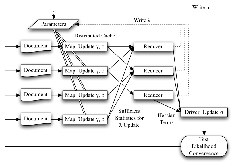
Figure 2: Workflow of Mr. LDA. Each iteration is broken into three stages: computing document-specific variational parameters in parallel mappers, computing topic-specific parameters in parallel reducers, and then updating global parameters in the driver, which also monitors convergence of the algorithm. Data flow is managed by the MapReduce framework: sufficient statistics from the mappers are directed to appropriate reducers, and new parameters computed in reducers are distributed to other computation units via the distributed cache.

The remainder of the paper focuses on adapting these updates into the MapReduce framework and challenges of working at a large scale. We focus on the primary components of a MapReduce algorithm: the mapper, which processes a single unit of data (in this case, a document); the reducer, which processes a single view of globally shared data (in this case, a topic parameter); the partitioner, which allows order inversion for normalization; and the driver, which controls the overall algorithm. The interconnections between the components of Mr. LDA are depicted in Figure 2.

3.1 Mapper: Update $\phi$ and $\gamma$

Each document has associated variational parameters $\gamma$ and $\phi$. The mapper computes the updates for these variational parameters and uses them to create the sufficient statistics needed to update the global parameters. In this section, we describe the computation of these variational updates and how they are transmitted to the reducers.

Given a document, the updates for $\phi$ and $\gamma$ are

$$\phi_{v,k}\propto\mathbb{E}_{q}\left[\beta_{v,k}\right]\cdot e^{\Psi\left(\textstyle\gamma_{k}\right)},\phantom{spac}\gamma_{k}=\alpha_{k}+\sum_{v=1}^{V}\phi_{v,k},$$

where $v\in[1,V]$ is the term index and $k\in[1,K]$ is the topic index. In this case, $V$ is the size of the vocabulary $\mathcal{V}$ and $K$ denotes the total number of topics. The expectation of $\beta$ under $q$ gives an estimate of how compatible a word is with a topic; words highly compatible with a topic will have a larger expected $\beta$ and thus higher values of $\phi$ for that topic.

Algorithm 1 illustrates the detailed procedure of the Map function. In the first iteration, mappers initialize variables, e.g. seed $\lambda$ with the counts of a single document. For the sake of brevity, we omit that step here; in later iterations, global parameters are stored in distributed cache – a synchronized read-only memory that is shared among all mappers [33] – and retrieved prior to mapper execution.

A document is represented as a term frequency sequence $\vec{w}=\|w_{1},w_{2},\ldots,w_{V}\|$, where $w_{i}$ is the corresponding term frequency in document $d$. For ease of notation, we assume the input term frequency vector $\vec{w}$ is associated with all the terms in the vocabulary, i.e., if term $t_{i}$ does not appear at all in document $d$, $w_{i}=0$.

Because the document variational parameter $\gamma$ and the word variational parameter $\phi$ are tightly coupled, we impose a local convergence requirement on $\gamma$ in the Map function. This means that the mapper alternates between updating $\gamma$ and $\phi$ until $\gamma$ stops changing.

Algorithm 1 Mapper

Input:
Key - document ID $d\in[1,C]$, where $C=|\mathcal{C}|$.
Value - document content.

Map

1:  Initialize a zero $V\times K$-dimensional matrix $\phi$.

2:  Initialize a zero $K$-dimensional row vector $\sigma$.

3:  Read in document content $\|w_{1},w_{2},\ldots,w_{V}\|$

4:  repeat

5:     for all $v\in[1,V]$ do

6:        for all $k\in[1,K]$ do

7:           Update $\phi_{v,k}=\frac{\lambda_{v,k}}{\sum_{v}{\lambda_{v,k}}}\cdot\exp(\Psi\left(\textstyle\gamma_{d,k}\right))$.

8:        end for

9:        Normalize $\phi_{v}$, set $\sigma=\sigma+w_{v}\phi_{v,*}$

10:     end for

11:     Update row vector $\gamma_{d,*}=\alpha+\sigma$.

12:  until convergence

13:  for all $k\in[1,K]$ do

14:     for all $v\in[1,V]$ do

15:        Emit $\langle k,\triangle\rangle:w_{v}\phi_{v,k}$. {Section 3.2}

16:        Emit $\langle k,v\rangle:w_{v}\phi_{v,k}$. {order inversion}

17:     end for

18:     Emit $\langle\triangle,k\rangle:(\Psi\left(\textstyle\gamma_{d,k}\right)-\Psi\left(\textstyle\sum_{l=1}^{K}\gamma_{d,l}\right))$. {$\alpha$ update, Section 3.4}

19:     Emit $\langle k,d\rangle-\gamma_{d,k}$ to file.

20:  end for

21:  Emit $\langle\triangle,\triangle\rangle-\mathcal{L}$ {ELBO, Section 3.5}

3.2 Partitioner: Efficient Marginal Sums

The Map function in Algorithm 1 emits sufficient statistics, which we will need to compile and normalize. To take advantage of the MapReduce framework to handle this computation, we use the order inversion design pattern [34, 35].

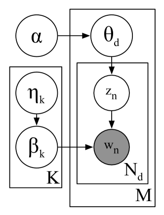
(a) LDA

(b) Variational

Figure 1: Graphical model of LDA and the mean field variational distribution. Each latent variable, observed datum, and parameter is a node. Lines between represent possible statistical dependence. Shaded nodes are observations; rectangular plates denote replication; and numbers in the bottom right of a plate show how many times plates’ contents repeat. In the variational distribution (Figure 1(b)), the latent variables $\theta$, $\beta$, and $z$ are explained by a simpler, fully factorized distribution with variational parameters $\gamma$, $\lambda$, and $\phi$. The lack of inter-document dependencies in the variational distribution allows the parallelization of inference in the MapReduce.

The sufficient statistics are keyed by a composite key set $\langle p_{\mathsf{left}},p_{\mathsf{right}}\rangle$. It is normally a pair of topic and word identifier. There are three exceptions:

• In addition to the vocabulary terms, we choose a special normalization key value (denoted by $\triangle$) that comes before any “normal” vocabulary key, i.e., $\triangle<v,\forall v\in[1,V]$. Before any word tokens are seen by the reducer, the reducer can compute the normalization term – by summing all of the values associated with $\triangle$ – and afterward write the final parameter values in a single pass through the reducer’s keys.

• If the value represents the sufficient statistics for $\alpha$ updating, the key pair is $\triangle$ and a topic identifier. The MapReduce framework ensures those keys arrive in lexicographic sorted order.

• Finally, if both keys are $\triangle$, it represents a document’s contribution to the likelihood bound $\mathcal{L}$; this is combined with the topic’s contribution.

This assumes that, for calculating a new parameter, a single reducer will see both the normalization key and all word keys. This is accomplished by ensuring the partitioner sorts on topic only. Thus, any reducers beyond the number of topics is superfluous. Given that the vast majority of the work is in the mappers, this is typically not an issue for LDA.

3.3 Reducer: Update $\lambda$

The Reduce function updates the variational parameter $\lambda$ associated with each topic. Because of the order inversion described above, the update is straightforward. It requires aggregation over all intermediate $\phi$ vectors

$$\lambda_{v,k} =\eta_{v,k}+\sum_{d=1}^{C}(w^{(d)}_{v}\phi^{(d)}_{v,k}),$$

where $d\in[1,C]$ is the document index and $w^{(d)}_{v}$ denotes the number of appearances of term $v$ in document $d$. Similarly, $C$ is the number of documents.

This is elaborated in Algorithm 2; Step 10 completes the final procedure for the order inversion design pattern – collecting all the marginal distribution counts. These aggregations will then be written to parameter files that will be used in subsequent iterations. Step 15 adds the contribution of the topic to the overall likelihood.

Algorithm 2 Reducer

Input:
Key - key pair $\langle p_{\mathsf{left}},p_{\mathsf{right}}\rangle$.
Value - an iterator $\mathcal{I}$ over sequence of values.

Reduce

1:  Compute the sum $\sigma$ over all values in the sequence $\mathcal{I}$.

2:  if $p_{\mathsf{left}}=\triangle$ then

3:     if $p_{\mathsf{right}}=\triangle$ then

4:        $\tau=\tau+\sigma$ {ELBO $\mathcal{L}$}

5:     else

6:        Emit $\langle\triangle,p_{\mathsf{right}}\rangle:\sigma$ {$\alpha$ update, Section 3.4}

7:     end if

8:  else

9:     if $p_{\mathsf{right}}=\triangle$ then

10:        Normalizer $\nu=\sigma+\sum_{v}\eta_{v,k}$. {order inversion}

11:        $\tau=\tau-\log\Gamma\left(\textstyle\nu\right)$

12:     else

13:        $\lambda_{v,k}=\eta_{v,k}+\sigma$

14:        Emit $\langle k,v\rangle:\frac{\lambda_{v,k}}{\nu+\sum_{j}\eta_{j,k}}$. {normalized $\mathbb{E}_{q}\left[\beta\right]$ value}

15:        $\tau=\tau+\log\Gamma\left(\textstyle\lambda_{v,k}\right)+\left(\lambda_{v,k}-1\right)\left(\Psi\left(\textstyle\lambda_{v,k}\right)-\Psi\left(\textstyle\nu\right)\right)$

16:     end if

17:  end if

18:  Emit $\langle\triangle,\triangle\rangle:\tau$

To improve performance, we use combiners to facilitate the aggregation of sufficient statistics in mappers before they were transferred to reducers. This decreases bandwidth and saves the reducer computation.

3.4 Driver: Update $\alpha$

Effective inference of topic models depends on learning not just the latent variables $\beta$, $\theta$, and $z$ but also estimating the hyperparameters, particularly $\alpha$. The $\alpha$ parameter controls the sparsity of topics in the document distribution and is the primary mechanism that differentiates LDA from previous models like pLSA and LSA; not optimizing $\alpha$ risks learning suboptimal topics [30].

Updating hyperparameters is also important from the perspective of equalizing differences between inference techniques; as long as hyperparameters are optimized, there is little difference between the output of inference techniques [36].

The driver program marshals the entire inference process. On the first iteration, the driver is responsible for initializing all the model parameters ($K$, $V$, $C$, $\eta$, $\alpha$); the number of topics $K$ is user specified; $C$ and $V$, the number of documents and types, is determined by the data; the initial value of $\alpha$ is specified by the user; and $\lambda$ is randomly initialized or seeded by documents.

3.5 Likelihood Computation

The driver monitors the ELBO to determine whether inference has converged. If not, it restarts the process with another round of mappers and reducers. To compute the ELBO we expand Equation 1, which gives us

$$\mathcal{L}(\gamma,\phi,\lambda;\alpha,\eta)= \underbrace{\sum_{d=1}^{C}\Phi(\alpha)}_{\mbox{\footnotesize{\footnotesize{driver}}}}+\underbrace{\sum_{d=1}^{C}(\underbrace{\mathcal{L}_{d}(\gamma,\phi)+\mathcal{L}_{d}(\phi)-\Phi(\gamma)}_{\mbox{\footnotesize{\footnotesize{computed in mapper}}}})}_{\mbox{\footnotesize{\footnotesize{computed in reducer}}}}$$

$$+\underbrace{\sum_{k=1}^{K}\Phi(\eta_{*,k})}_{\mbox{\footnotesize{\footnotesize{driver / constant}}}}-\underbrace{\sum_{k=1}^{K}\underbrace{\Phi(\lambda_{*,k})}_{\mbox{\footnotesize{\footnotesize{reducer}}}}}_{\mbox{\footnotesize{\footnotesize{driver}}}}$$

where

$$\Phi(\mu)= \log\Gamma\left(\textstyle\sum_{i=1}\mu_{i}\right)-\sum_{i=1}\log\Gamma\left(\textstyle\mu_{i}\right)$$

$$+\sum_{i}\left(\mu_{i}-1\right)\left(\Psi\left(\textstyle\mu_{i}\right)-\Psi\left(\textstyle\sum_{j}\mu_{j}\right)\right).$$

$$\mathcal{L}_{d}(\gamma,\phi)= \sum_{k=1}^{K}\sum_{v=1}^{V}\phi_{v,k}w_{v}\left[\Psi\left(\textstyle\gamma_{k}\right)-\Psi\left(\textstyle\sum_{i=1}^{K}\gamma_{i}\right)\right],$$

$$\mathcal{L}_{d}(\phi)= \sum_{v=1}^{V}\sum_{k=1}^{K}\phi_{v,k}\left(\sum_{i=1}^{V}w_{i}\log\frac{\lambda_{i,k}}{\sum_{j}\lambda_{j,k}}-\log\phi_{v,k}\right),$$

Almost all of the terms that appear in the likelihood term can be computed in mappers; the only term that cannot are the terms that depend on $\alpha$, which is updated in the driver, and the variational parameter $\lambda$, which is shared among all documents. All terms that depend on $\alpha$ can be easily computed in the driver, while the terms that depend on $\lambda$ can be computed in each reducer.

Thus, computing the total likelihood proceeds as follows: each mapper computes its contribution to the likelihood bound $\mathcal{L}$, and emits a special key that is unique to likelihood bound terms and then aggregated in the reducer; the reducers add topic-specific terms to the likelihood; these final values are then combined with the contribution from $\alpha$ in the driver to compute a final likelihood bound.

The driver updates $\alpha$ after each MapReduce iteration. We use a Newton-Raphson method which requires the Hessian matrix and the gradient,

$$\alpha_{\mathsf{new}}=\alpha_{\mathsf{old}}-\mathcal{H}^{-1}(\alpha_{\mathsf{old}})\cdot g(\alpha_{\mathsf{old}}),$$

where the Hessian matrix $\mathcal{H}$ and $\alpha$ gradient are defined respectively as

$$\mathcal{H}(k,l)= \delta(k,l)C\Psi^{\prime}\left(\textstyle\alpha_{k}\right)-C\Psi^{\prime}\left(\textstyle\sum_{l=1}^{K}\alpha_{l}\right),$$

$$g(k)= \underbrace{C\left(\Psi\left(\textstyle\sum_{l=1}^{K}\alpha_{l}\right)-\Psi\left(\textstyle\alpha_{k}\right)\right)}_{\mbox{\footnotesize{\footnotesize{computed in driver}}}}+$$

$$\underbrace{\sum_{d=1}^{C}\underbrace{\Psi\left(\textstyle\gamma_{d,k}\right)-\Psi\left(\textstyle\sum_{l=1}^{K}\gamma_{d,l}\right)}_{\mbox{\footnotesize{\footnotesize{computed in mapper}}}}}_{\mbox{\footnotesize{\footnotesize{computed in reducer}}}}.$$

The Hessian matrix $\mathcal{H}$ depends entirely on the vector $\alpha$, which changes during updating $\alpha$. The gradient $g$, on the other hand, can be decomposed into two terms: the $\alpha$-tokens (i.e., $\Psi\left(\textstyle\sum_{l=1}^{K}\alpha_{l}\right)-\Psi\left(\textstyle\alpha_{k}\right)$) and the $\gamma$-tokens (i.e., $\sum_{d=1}^{C}\Psi\left(\textstyle\gamma_{d,k}\right)-\Psi\left(\textstyle\sum_{l=1}^{K}\gamma_{d,l}\right)$). We can remove dependence on the number of documents in the gradient computation by computing the $\gamma$-tokens in mappers. This key observation allows us to optimize $\alpha$ in the MapReduce environment.

Because LDA is a dimensionality reduction algorithm, there are typically a small number of topics $K$ even for a large document collection. As a result, we can safely assume the dimensionality of $\alpha$, $\mathcal{H}$, and $g$ are reasonably low, and additional gains come from the diagonal structure of the Hessian [37]. Hence, the updating of $\alpha$ is efficient and will not create a bottleneck in the driver.

4 Flexibility of Mr. LDA

In this section, we highlight the flexibility of Mr. LDA to accomodate extensions to LDA. These extensions are possible because of the modular nature of Mr. LDA’s design.

4.1 Informed Prior

The standard practice in topic modeling is to use a same symmetric prior (i.e. $\eta_{v,k}$ is the same for all topics $k$ and words $v$). However, the model and inference presented in Section 3 allows for topics to have different priors; allowing users to incorporate prior information into the model.

For example, suppose our we wanted to discover how different psychological states were expressed in blogs or newspapers. If this were our goal, we might reasonably create priors that captured psychological categories to discover how they were expressed in a corpus. The Linguistic Inquiry and Word Count (LIWC) dictionary [38] defines 68 categories encompassing psychological constructs and personal concerns. For example, the anger LIWC category includes the words “abuse,” “jerk,” and “jealous;” the anxiety category includes “afraid,” “alarm,” and “avoid;” and the negative emotions category includes “abandon,” “maddening,” and “sob.” Using this dictionary, we built a prior ${\bm{\eta}}$ as follows:

$$\eta_{v,k}=\begin{cases}10,\text{ if }v\in\mbox{LIWC category}_{k}\\ 0.01,\text{ otherwise}\end{cases},$$

where $\eta_{v,k}$ is the informed prior for word $v$ of topic $k$. This is accomplished via a slight modification of the reducer and leaving the rest of the system unchanged.

4.2 Polylingual LDA

In this section, we demonstrate the flexibility of Mr. LDA by showing how its component-based design allows for extending LDA beyond a single language. PolyLDA [12] assumes a document-aligned multilingual corpus. For example, articles in Wikipedia have links to the version of the article in other languages; while the linked documents are ostensibly on the same subject, they are usually not direct translations, and possibly written to have a culture-specific focus.

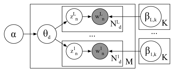
Figure 3: Graphical model for polylingual LDA [12]. Each document has words in multiple languages. Inference learns the common topic ids across languages that co-occur in the corpus. The modular inference of Mr. LDA allows for inference for this model to be accomplished by the same framework created for monolingual LDA.

PolyLDA assumes that a single document has words in multiple languages, but each document has a common, language agnostic per-document distribution $\theta$ (Figure 3). Each topic also has different facets for language; these topics end up being consistent because of the links across language encoded in the consistent themes present in documents.

Because of the modular way in which we implemented inference, we can perform multilingual inference by embellishing each data unit with a language identifier $l$ and change inference as follows:

• Updating $\lambda$ happens $l$ times, one for each language. The updates for a particular language ignores expected counts of all other languages.

• Updating $\phi$ happens using only the relevant language for a word.

• Updating $\gamma$ happens as usual, combining the contributions of all languages relevant for a document.

From an implementation perspective, PolyLDA is a collection of monolingual Mr. LDA computations sequenced appropriately. Mr. LDA’s approach of taking relatively simple computation units, allowing them to scale, and preserving simple communication between computation units stands in contrast to the design choices by approaches using Gibbs sampling.

For example, Smola and Narayanamurthy [21] interleave the topic and document counts during the computation of the conditional distribution using Yao et al.’s “binning” approach [39]. While this improves performance, changing any of the modeling assumptions would potentially break this optimization.

In contrast, Mr. LDA’s philosophy allows for easier development of extensions of LDA. While we only discuss two extensions here, other extensions are possible. For example, implementing supervised LDA [40] only requires changing the computation of $\phi$ and a regression; the rest of the model is unchanged. Implementing syntactic topic models [41] requires changing the mapper to incorporate syntactic dependencies.

5 Experiments

We implemented Mr. LDA using Java with Hadoop 0.20.1 and ran it on a cluster provided by NSF’s CLUster Exploratory Program (CluE) and the Google/IBM Academic Cloud Computing Initiative. The cluster used in our experiments contained 280 physical nodes; each node has two single-core processors (2.8 GHz), 4 GB memory, and two 400 GB hard drives. The cluster was configured to run a maximum of three map tasks and two reduce tasks simultaneously, and usually under a heavy, heterogeneous load.

5.1 Scalability

We report results on the TREC document collection (disks 4 and 5 [42]), consisting mostly of newswire documents from the Financial Times and LA Times. It contains more than $100,000$ distinct word types in approximately half a million documents. As a preprocessing step, we remove types that appear fewer than $20$ times and apply stemming [43], reducing the vocabulary size to approximately $65,000$. This speeds inference and is consistent with standard approaches for LDA (but with a larger vocabulary than is typical).

Figure 4 shows the relationship between training time and corpus size the training time averaged over the first 20 Map/Reduce iterations. For this experiment, the number of topics was set to $K=10$, and inference was done with 137 mappers (the number of input sequence files) and 100 reducers. Doubling the corpus size results in a less than 20% increase increase in running time, suggesting that Mr. LDA is able to successfully distribute the workload to more machines and take advantage of parallelism. As the number of input documents increases, the training time increases gracefully.

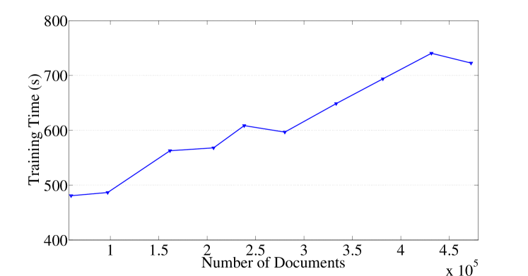
Figure 4: Scalability vs. No. of Input Documents. The average training time increases in an approximately linear fashion, as the number of input documents increases. This suggests Mr. LDA is parallelizing effectively as more computing resources are available.

The number of topics is another important factor affecting the training time (and hence the scalability) of the model. Figure 5 shows the average time for one iteration against different numbers of topics. In this experiment, we use $10\%$ data (over $40k$ documents) to train, and the time is measured after model convergence. As the number of topics we want to model increases, the training time for every iteration also increases, as additional machines take up the additional load.

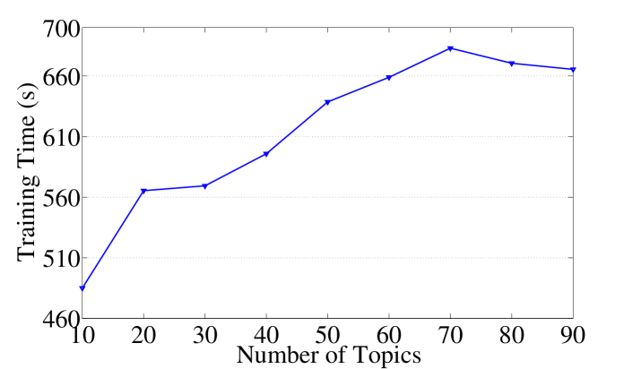
Figure 5: Scalability vs. Number of Topics. As we increase the number of topics, the average training time also increases gradually.

Ideally, these increases should be perfectly linear with the size of input and/or number of topics. However, MapReduce framework involves machine cycle scheduling, data load balance, and disk I/O operations between each iteration. These factors highly rely on the underlying hardware and network.

The synchronization overhead of MapReduce is related to the number of keys emitted by mappers and ability of the cluster to transmit and process these data. In Mr. LDA, every mapper emits $O(T_{d}K)$ messages, where $T_{d}$ is the number of types in document $d$ and $K$ is the number of topics (in practice, it could be less, as combiners can combine messages within mappers). To empirically validate this linear growth in both data size and the complexity of the model, we ran Mr. LDA on the entire dataset with $100$ topics and $10$ topics. The intermediate data shuffled by the platform is approximately $10$ times larger – $6.470$ GB ($466.60$ million records) for $100$ topics vs. $646.79$ MB ($46.66$ million records) for $10$ topics. Combiners in both cases help to reduce the intermediate data significantly. In the $100$ topics scenario, combiners merge more than $16$ billion key value pairs at the mapper side, whereas for $10$ topics case, they merge slightly more than $1.6$ billion records.

To better test the scalability of our implementation, we further measure the training time under different numbers of mappers. Again, the training time is measured over $20$ EM iterations and the number of topics is set to $10$. Total number of input documents is $472525$.

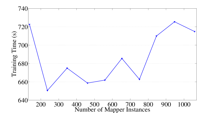
Figure 6: Scalability vs. Number of Mapper Instances. The number of mapper instances represents a trade-off between number of processing units and network traffic due to intermediate data transfer. A larger number of mappers provides more computational resources, but also creates network congestion during system shuffling and sorting.

As illustrated in Figure 6, we observe that training time first decreases as we increase the number of mappers. Eventually, for a fixed number of documents, adding additional mappers increases the computation time. This is because each mapper processes fewer documents but still has fixed startup costs and because more mappers generate greater network congestion (fewer opportunities to combine results). As with many MapReduce algorithms, one must choose the correct amount of resources to solve a problem.

While the number of reducers is important in general, the majority of the work in Mr. LDA is done in the mappers. Therefore, the number of map tasks depends on the size of the corpus; however, a single reducer, with a pass through the vocabulary, is comparatively simple. As long as the number of reducer instances is greater than the number of topics, reducers will not be a significant bottleneck.

If we assume all the topics are used, which is generally true in LDA, we will have subsets with approximately equal size. Hence, the entire workload will be distributed somewhat evenly among all reducer instances. In this case, it is unlikely that one reducer will delay the termination of the MapReduce step. This is further assisted by the use of combiners, which can preemptively do some of the reducers’ work.

5.2 Held-out Likelihood

Unlike the Gibbs sampling algorithms discussed in Section 2.1, which sacrifice the semantics of inference to improve scalability, Mr. LDA’s inference is identical to that conducted on a single machine. Thus, there is no need to compare likelihood against stand-alone implementations. However, It is useful to examine likelihood to determine the number of iterations (and synchronizations) necessary for inference.

Figure 7 shows the training likelihood against the number of iterations. To ease comparisons between different numbers of topics, the likelihood has been divided by the final likelihood bound value. The legend shows the number of topics and number of iterations to converge. For example, if we want to train $30$ topics on the training dataset, it would take $25$ iterations to converge. More complex models with more topics understandably require more iterations to converge. While this is common knowledge (and independent of MapReduce), we stress this point because of its contrast with Gibbs sampling, which typically takes hundreds of iterations or more to converge [21] with substantially more synchronizations required. When the expensive computations can be easily parallelized, as is the case with both Gibbs sampling and variational inference, one should try to minimize the number of steps where an explicit synchronization must take place.

Figure 7: Normalized Training Likelihood vs. Number of Topics. Here, the likelihood is scaled by the likelihood bound at convergence so that we can compare different number of topics. The iteration at which the model converged is shown in the legend as $I$. Generally, more topics require more iterations for the algorithm to converge, but the number of iterations is in the dozens rather than in the hundreds (as with Gibbs sampling).

5.3 Informed Priors

In this set of experiment, we build the informed priors from LIWC [38] dictionary as we discussed in Section 4.1. Besides TREC dataset, we also used the same informed prior on the BlogAuthorship corpus [44], which contains about 10 million blog posts from American users. In contrast to the newswire-heavy TREC corpus, the BlogAuthorship corpus is more personal and informal. Again, terms in fewer than $20$ documents are excluded, resulting $53000$ types. Throughout the experiments, we set the number of topics to 100, with $12$ guided by the informed prior.

The results are shown in Table 2. The prior acts as a seed, causing words used in similar contexts to become part of the topic. This is important for computational social scienctists who want to discover how an abstract idea (represented by a set of words) is actually expressed in a corpus. For example, public news media (e.g., news articles like TREC) relates positive emotions to entertainment, such as music, film and TV, whereas social media (e.g., blog posts) relates it to religion. The Anxiety topic in news relates to middle east, but in blogs, it focuses on illness, e.g. bird flu. In both corpora, Causation was linked to science.

Using informed priors can discover radically different words. While LIWC is designed for relatively formal writing, it can also discover Internet slang such as “lol” (“laugh out loud”) in Affective Process category. On the other hand, some discovered topics do not have a clear relationship with the initial LIWC categories, such as the abbreviations and acronyms in Discrepancy category.

	Affective Processes	Negative Emotions	Positive Emotions	Anxiety	Anger	Sadness	Cognitive Processes	Insight	Causation	Discrepancy	Tentative	Certainty
Output from TREC	book	fire	film	al	polic	stock	coalit	un	technolog	pound	hotel	art
	life	hospit	music	arab	drug	cent	elect	bosnia	comput	share	travel	italian
	love	medic	play	israel	arrest	share	polit	serb	research	profit	fish	itali
	like	damag	entertain	palestinian	kill	index	conflict	bosnian	system	dividend	island	artist
	stori	patient	show	isra	prison	rose	anc	herzegovina	electron	group	wine	museum
	man	accid	tv	india	investig	close	think	croatian	scienc	uk	garden	paint
	write	death	calendar	peac	crime	fell	parliament	greek	test	pre	design	exhibit
	read	doctor	movie	islam	attack	profit	poland	yugoslavia	equip	trust	boat	opera
Output from Blog	easili	sorri	lord	bird	iraq	level		god	system	sa	pretty	film
	dare	crappi	prayer	diseas	american	weight		christian	http	ko	davida	actor
	truli	bullshit	pray	shi	countri	disord		church	develop	ang	croydon	robert
	lol	goddamn	merci	infect	militari	moder		jesus	program	pa	crossword	william
	needi	messi	etern	blood	nation	miseri		christ	www	ako	chrono	truli
	jealousi	shitti	truli	snake	unit	lbs		religion	web	en	jigsaw	director
	friendship	bitchi	humbl	anxieti	america	loneli		faith	file	lang	40th	charact
	betray	angri	god	creatur	force	pain		cathol	servic	el	surrey	richard

Table 2: Twelve Topics Discovered from TREC (top) and BlogAuthorship (bottom) collection with LIWC-derived informed prior. The model associates TREC documents containing words like “arab”, “israel”, “palestinian” and “peace” with Anxiety. In the blog corpus, however, the model associates words like “iraq”,“america*”, “militari”, “unit”, and “force” with the Anger category.

5.4 Polylingual LDA

As discussed in Section 4.2, Mr. LDA’s modular design allows us to consider models beyond vanilla LDA. Using what we believe is the first framework for variational inference for polylingual LDA [12], we fit $50$ topics to paired English and German Wikipedia articles (approximately $500$k in each language). As before, we ignore terms appearing in fewer than $20$ documents, resulting in $170$k English word types and $210$k German word types. While each pair of linked documents shares a common subject (e.g. “George Washington”), they are usually not direct translations. We let the program run for $33$ iterations with $100$ mappers and $50$ reducers; Table 3 lists down some words from a set of randomly chosen topics.

English	game	opera	greek	league	said	italian	soviet	french	japanese	album	york	professor
	games	musical	turkish	cup	family	church	political	france	japan	song	canada	berlin
	player	composer	region	club	could	pope	military	paris	australia	released	governor	lied
	players	orchestra	hugarian	played	childern	italy	union	russian	australian	songs	washington	germany
	released	piano	wine	football	death	catholic	russian	la	flag	single	president	von
	comics	works	hungary	games	father	bishop	power	le	zealand	hit	canadian	worked
	characters	symphony	greece	career	wrote	roman	israel	des	korea	top	john	studied
	character	instruments	turkey	game	mother	rome	empire	russia	kong	singer	served	published
	version	composers	ottoman	championship	never	st	republic	moscow	hong	love	house	received
	play	performed	romania	player	day	ii	country	du	korean	chart	county	member
Germany	spiel	musik	ungarn	saison	frau	papst	regierung	paris	japan	album	new	berlin
	spieler	komponist	turkei	gewann	the	rom	republik	franzosischen	japanischen	the	staaten	universitat
	serie	oper	turkischen	spielte	familie	ii	sowjetunion	frankreich	australien	platz	usa	deutschen
	the	komponisten	griechenland	karriere	mutter	kirche	kam	la	japanische	song	vereinigten	professor
	erschien	werke	rumanien	fc	vater	di	krieg	franzosische	flagge	single	york	studierte
	gibt	orchester	ungarischen	spielen	leben	bishof	land	le	jap	lied	washington	leben
	commics	wiener	griechischen	wechselte	starb	italien	bevolkerung	franzosischer	australischen	titel	national	deutscher
	veroffentlic	komposition	istanbul	mannschaft	tod	italienischen	ende	russischen	neuseeland	erreichte	river	wien
	2	klavier	serbien	olympischen	kinder	konig	reich	moskau	tokio	erschien	county	arbeitete
	konnen	wien	osmanischen	platz	tochter	kloster	politischen	jean	sydney	a	gouverneur	erhielt

Table 3: Extracted Polylingual Topics from the Wikipedia Corpus. While topics are generally equivalent (e.g. on “computer games” or “music”), some regional differences are expressed. For example, the “music” topic in German has two words referring to “Vienna” (“wiener” and “wien”), while the corresponding concept in English does not appear until the $15^{\text{th}}$ position.

6 Conclusion and Future Work

Understanding large text collections such as those generated via social media requires algorithms that are unsupervised and scalable. In this paper, we present Mr. LDA, which fulfils both of these requirements. Beyond text, LDA has been successfully applied to other domains such as music [45], computer vision [2], biology [5], and source code [46]. All of these domains struggle with the scale of data, and Mr. LDA could help them better cope with large data.

Mr. LDA represents an alternative to the existing scalable mechanisms for inference of topic models. Its design easily accomodates other extensions, as we have demonstrated with the addition of informed priors and multilingual topic modeling, and the ability of variational inference to support non-conjugate distributions allows for the development of a broader class of models than could be built with Gibbs samplers alone. Mr. LDA, however, would benefit from many of the efficient, scalable datastructures that improved other scalable statistical models [47]; incorporating these insights would further improve performance and scalability.

While we focused on LDA, the approaches used here are applicable to many other models. Variational inference is an attractive inference technique for the MapReduce framework, as it allows the selection of a variational distribution that breaks dependencies among variables to enforce consistency with the computational constraints of MapReduce. Developing automatic ways to enforce those computational constraints and then automatically derive inference [48] would allow for a greater variety of statistical models to be learned efficiently in a parallel computing environment.

Variational inference is also attractive for its ability to handle online updates. Mr. LDA could be extended to more efficiently handle online batches in streaming inference [49], allowing for even larger document collections to be quickly analyzed and understood.

References

- [1] D. M. Blei, A. Ng, and M. Jordan, “Latent Dirichlet allocation,” JMLR, vol. 3, pp. 993–1022, 2003.
- [2] F. Rob, L. Fei-Fei, P. Pietro, and Z. Andrew, “Learning object categories from Google’s image search.” in ICCV, 2005.
- [3] C. Wang, D. Blei, and L. Fei-Fei, “Simultaneous image classification and annotation,” in CVPR, 2009.
- [4] E. M. Airoldi, D. M. Blei, S. E. Fienberg, and E. P. Xing, “Mixed membership stochastic blockmodels,” JMLR, vol. 9, pp. 1981–2014, 2008.
- [5] D. Falush, M. Stephens, and J. K. Pritchard, “Inference of population structure using multilocus genotype data: linked loci and correlated allele frequencies.” Genetics, vol. 164, no. 4, pp. 1567–1587, 2003.
- [6] J. Boyd-Graber and D. M. Blei, “Multilingual topic models for unaligned text,” in UAI, 2009.
- [7] T. L. Griffiths, M. Steyvers, D. M. Blei, and J. B. Tenenbaum, “Integrating topics and syntax,” in NIPS, 2005.
- [8] J. Dean and S. Ghemawat, “MapReduce: Simplified data processing on large clusters,” in OSDI, San Francisco, California, 2004, pp. 137–150.
- [9] C. Dyer, A. Cordova, A. Mont, and J. Lin, “Fast, easy and cheap: Construction of statistical machine translation models with MapReduce,” in Workshop on SMT (ACL 2008), Columbus, Ohio, 2008.
- [10] T. Brants, A. C. Popat, P. Xu, F. J. Och, and J. Dean, “Large language models in machine translation,” in EMNLP, 2007.
- [11] S. B. Cohen and N. A. Smith, “Shared logistic normal distributions for soft parameter tying in unsupervised grammar induction,” in NAACL, 2009.
- [12] D. Mimno, H. Wallach, J. Naradowsky, D. Smith, and A. McCallum, “Polylingual topic models,” in EMNLP, 2009, IR.
- [13] R. M. Neal, “Probabilistic inference using Markov chain Monte Carlo methods,” University of Toronto, Tech. Rep. CRG-TR-93-1, 1993.
- [14] C. Robert and G. Casella, Monte Carlo Statistical Methods, ser. Springer Texts in Statistics. New York, NY: Springer-Verlag, 2004.
- [15] Y. W. Teh, “A hierarchical Bayesian language model based on Pitman-Yor processes,” in ACL, 2006.
- [16] T. L. Griffiths and M. Steyvers, “Finding scientific topics,” PNAS, vol. 101, no. Suppl 1, pp. 5228–5235, 2004.
- [17] J. R. Finkel, T. Grenager, and C. D. Manning, “The infinite tree,” in ACL, 2007.
- [18] D. Newman, A. Asuncion, P. Smyth, and M. Welling, “Distributed Inference for Latent Dirichlet Allocation,” in NIPS, 2008.
- [19] F. Yan, N. Xu, and Y. Qi, “Parallel inference for latent dirichlet allocation on graphics processing units,” in NIPS, 2009, pp. 2134–2142.
- [20] Y. Wang, H. Bai, M. Stanton, W.-Y. Chen, and E. Y. Chang, “PLDA: parallel latent Dirichlet allocation for large-scale applications,” in AAIM, 2009.
- [21] A. J. Smola and S. Narayanamurthy, “An architecture for parallel topic models,” VLDB, vol. 3, 2010.
- [22] M. I. Jordan, Z. Ghahramani, T. S. Jaakkola, and L. K. Saul, “An introduction to variational methods for graphical models,” Machine Learning, vol. 37, no. 2, pp. 183–233, 1999.
- [23] M. J. Wainwright and M. I. Jordan, “Graphical models, exponential families, and variational inference,” Foundations and Trends in Machine Learning, vol. 1, no. 1–2, pp. 1–305, 2008.
- [24] D. M. Blei and M. I. Jordan, “Variational inference for Dirichlet process mixtures,” Journal of Bayesian Analysis, vol. 1, no. 1, pp. 121–144, 2005.
- [25] Y. W. Teh, M. I. Jordan, M. J. Beal, and D. M. Blei, “Hierarchical Dirichlet processes,” JASA, vol. 101, no. 476, pp. 1566–1581, 2006.
- [26] K. Kurihara, M. Welling, and N. Vlassis, “Accelerated variational Dirichlet process mixtures,” in NIPS, Cambridge, MA, 2007.
- [27] J. Wolfe, A. Haghighi, and D. Klein, “Fully distributed EM for very large datasets,” in ICML, 2008, pp. 1184–1191.
- [28] R. Nallapati, W. Cohen, and J. Lafferty, “Parallelized variational EM for latent Dirichlet allocation: An experimental evaluation of speed and scalability,” in ICDMW, 2007.
- [29] A. S. Foundation, I. Drost, T. Dunning, J. Eastman, O. Gospodnetic, G. Ingersoll, J. Mannix, S. Owen, and K. Wettin, “Apache Mahout,” 2010, http://mloss.org/software/view/144/.
- [30] H. Wallach, D. Mimno, and A. McCallum, “Rethinking LDA: Why priors matter,” in NIPS, 2009.
- [31] A. K. McCallum, “Mallet: A machine learning for language toolkit,” 2002, http://www.cs.umass.edu/ mccallum/mallet.
- [32] A. Asuncion, P. Smyth, and M. Welling, “Asynchronous distributed learning of topic models,” in NIPS, 2008.
- [33] T. White, Hadoop: The Definitive Guide (Second Edition), 2nd ed., M. Loukides, Ed. O’Reilly, 2010.
- [34] J. Lin and C. Dyer, Data-Intensive Text Processing with MapReduce, ser. Synthesis Lectures on Human Language Technologies. Morgan & Claypool Publishers, 2010.
- [35] C. Lin and Y. He, “Joint sentiment/topic model for sentiment analysis,” in CIKM, 2009.
- [36] A. Asuncion, M. Welling, P. Smyth, and Y. W. Teh, “On smoothing and inference for topic models,” in UAI, 2009.
- [37] T. P. Minka, “Estimating a dirichlet distribution,” Microsoft, Tech. Rep., 2000, http://research.microsoft.com/en-us/um/people/minka/papers/dirichlet/.
- [38] J. W. Pennebaker and M. E. Francis, Linguistic Inquiry and Word Count, 1st ed. Lawrence Erlbaum, August 1999.
- [39] L. Yao, D. Mimno, and A. McCallum, “Efficient methods for topic model inference on streaming document collections,” 2009.
- [40] D. M. Blei and J. D. McAuliffe, “Supervised topic models,” in NIPS. MIT Press, 2007.
- [41] J. Boyd-Graber and D. M. Blei, “Syntactic topic models,” in NIPS, 2008.
- [42] NIST, “Trec special database 22,” 1994, http://www.nist.gov/srd/nistsd22.htm.
- [43] M. Porter and R. Boulton, “Snowball stemmer,” 1970, http://snowball.tartarus.org/credits.php.
- [44] M. Koppel, J. Schler, S. Argamon, and J. Pennebaker, “Effects of age and gender on blogging,” in In AAAI 2006 Symposium on Computational Approaches to Analysing Weblogs, 2006.
- [45] D. Hu and L. K. Saul, “A probabilistic model of unsupervised learning for musical-key profiles,” in ISMIR, 2009.
- [46] G. Maskeri, S. Sarkar, and K. Heafield, “Mining business topics in source code using latent dirichlet allocation,” in ISEC, 2008.
- [47] D. Talbot and M. Osborne, “Smoothed bloom filter language models: Tera-scale lms on the cheap,” in ACL, 2007, pp. 468–476.
- [48] J. Winn and C. M. Bishop, “Variational message passing,” JMLR, vol. 6, pp. 661–694, 2005.
- [49] M. Hoffman, D. M. Blei, and F. Bach, “Online learning for latent dirichlet allocation,” in NIPS, 2010.