The long-term cyclotron dynamics of relativistic wave packets: spontaneous collapse and revival

Abstract

In this work we study the effects of collapse and revival as well as Zitterbewegung (ZB) phenomenon, for the relativistic electron wave packets, which are a superposition of the states with quantum numbers sharply peaked around some Landau level $n_{0}$ of the order of few tens. The probability densities as well as average velocities of the packet center and the average spin components were calculated analytically and visualized. Our computations demonstrate that due to dephasing of the states for times larger than the cyclotron period the initial wave packet (which includes the states with the positive energy only) loses the spatial localization so that the evolution can no longer be described classically. However, at the half-revival time $t=T_{R}/2$ its reshaping takes place firstly. The behavior of the wave packet containing the states of both energy bands (with $E_{n}>0$ and $E_{n}<0$) is more complicated. At short times of a few classical periods such packet splits into two parts which rotate with cyclotron frequency in the opposite directions and meet each other every one-half of the cyclotron period. At these moments their wave functions have significant overlap that leads to ZB. At the time of fractional revival each of two sub-packets is decomposed into few packet-fractions. However, at $t=T_{R}$ each of the two sub-packets (with positive or negative energy) restores at various points of the cyclotron orbit, that makes it impossible reshaping of initial wave packet entirely unlike the wave packet which consists of states with energies $E_{n}>0$ only. Obtained results can be useful for the description of electromagnetic radiation and absorption in relativistic plasma on astrophysics objects, where super high magnetic field has the value of the order $10^{8}-10^{9}$T, as well as for interpretation of experiments with trapped ions.

I Introduction

The space-time evolution of quantum system with discrete but not equidistant energy spectrum can be quite complex. It was shownA1 that for the initial state consisting of the eigenstates with quantum numbers $n$ sharply peaked around some level $n_{0}\gg 1$ the coefficients of Taylor expansion of spectrum $E_{n}$ around that value define the different time scales of wave packet periodic evolution.

At the beginning a localized wave packet moves periodically along a classical trajectory with the period $T_{cl}=2\pi\hbar/E^{\prime}_{n_{0}}$. However, over time, the nonlinear terms in $(n-n_{0})$ in the expansion of the spectrum $E_{n}$ become significant, resulting in a spreading of the packet. The next stage of a long-term evolution of semiclassical wave packets for a large class of quantum systems is universal as was shown in Ref.A1 . Thus, at the revival time $T_{R}=4\pi\hbar/E^{\prime\prime}_{n_{0}}$ the additional phases of the individual components of the wave packet due to quadratic terms in the expansion are exactly multiplied by $2\pi$ which means a full reshaping of the wave packet. At the times of fractional revivals $t=mT_{R}/n$, where $m$ and $n$ are mutually prime integers, the phase differences between subsets of the component eigenfunctions are stationary, and the wave packet breaks up into sets of sub-packets. After a few revivals one obtains a complicated distribution of probability density around the classical trajectory.

During some past decades the phenomena of collapse and revival have been investigated theoretically and experimentally in different quantum systems. In particular, revivals and fractional revivals have been investigated theoretically for Ridberg atoms, molecules and in low dimensional quantum structures. Firstly, the detailed calculation of a short laser pulse exitation of the high-energies Rydberg states and the total power radiated by the atom was performed in Ref.Par . The space-time dynamics of the hydrogen atom was considered in Ref.Dac by constructing a minimum-uncertainty wave packet that travels along a kepler orbit. It was shown that both classical and quantum properties associated with the discreteness and non-equidistance of the atomic spectrum occur inevitably in the long-term evolution of wave packets. Romera and SantosRom studied the cyclotron dynamics of electrons in a monolayer graphene, where low energy excitations are massless Dirac fermions. They showed that when electrons are described by wave packets with a Gaussian population of only positive energy Landau levels, the presence of the magnetic field induces revivals of the electron currents, besides the classical cyclotron motion. When the population comprises both positive and negative energy Landau levels, revivals of the electric charge current manifest simultaneously with Zitterbewegung (ZB) and the classical cyclotron motion. In Ref.Tor the quasiclassical evolution as well as the phenomenon of collapse and revival of a wave packets in graphene quantum dots in a perpendicular magnetic field was studied.

The Dirac equation also predicts an unexpected features of relativistic motion. Bermudes et al.Berm considered the evolution of relativistic wave packets in a magnetic field and predicted three regimes: macroscopic, microscopic and mesoscopic (intermediate) when the electron energy level comprises several tens of Landau levels. The authors of Ref.Berm applied an exact mapping between relativistic model and a combination of Jaynes-Cummings and anti-Jaynes-Cummings interactionsJC widely used by the quantum optics community. In the work Berm the relativistic version of ”Schrödinger cat” states, or ”Dirac cat” states, was built for relativistic Landau levels when an external magnetic field couples the states of a relativistic spin $1/2$ charged particle.

Rusin and ZawadzkiRZ considered the effect of trembling motion of wave packet center or ZB for relativistic electrons moving in a vacuum in the presence of an external magnetic field. As in the original work by SchrödingerSh they used one-electron approximation and found that in this case the effect of ZB is very small. The authors of Ref.RZ noted, that in accordance with results obtained by KrekoraKre , the fully occupied electron negative energy states, or Dirac vacuum, may prevent the interference and ZB to occur. For this reason the Zitterbewegung is merely a mathematical property of the one-electron Dirac equation and can not be observed for real electrons. So, the calculations in Ref.RZ were made for 2+1 and 3+1 Dirac equations for parameters, which correspond to the motion of trapped ions in recent experiments by Gerritsma and coworkersGer .

Gea-Banacloche evaluated the asymptotic description for the evolution of two-level atom interacting with a quantized field in initially coherent stateGea . The collapse and revival was investigated in this system. It was stated that collapse appears to be associated with a measurement of the initial state of the atom with the field. At the half-revival time the pure state of the field, which is a mesoscopic superposition of coherent states, is referred to as a ”Schrödinger cat”.

The phenomena of collapse and revival was observed experimentally in different nonlinear quantum models. Among them, the two-level atom trapped in a high-Q microwave cavityAuf , Rydberg wave packets in atomYea and molecular vibrational states.Vra Interestingly, methods for laser isotope separation which take advantage of the revival phenomenon, were proposed and realized in Ref.A2 . In experiment Monroe et allMon a superposition of two different coherent states was created for an ion oscillating in a harmonic potential.

The quantum dynamics of free relativistic particles represented by three-dimensional Gaussian wave packets with different initial spin polarizations was investigated and visualized in Ref.DMPF . The influence of the symmetry of the initial wave packet on its kinematic characteristics such as average electron velocity, the direction of trembling motion as well as the distribution of spin densities was analyzed also. The effects of splitting and ZB of electron wave packets in the semiconductor quantum well under the influence of the Rashba spin orbit coupling and also in monolayer graphene were considered in Refs.DMF ; MDF .

In this work we study the long-term cyclotron dynamics of relativistic electrons, which obey the Dirac equation. For this purpose we use the inertial frame in which the component of momentum parallel to the direction of the magnetic field equals to zero. Such choice allows to represent the most of results in the clear analytical form. To describe the behavior of the relativistic particle we consider the superposition of the eigenstates of the Dirac Hamiltonian which is centered around some quantum number $n_{0}\gg 1$. The bispinor structure of electron wave function and existence of two energy bands lead to a quite complex dynamics of wave packets. The space-time evolution of electron probability densities, as well as spin densities was investigated analytically and numerically and after that visualized.

The paper is organized as follows. In Sec. II the relativistic electron eigenstates and eigenvalues of Dirac Hamiltonian in a magnetic field are introduced and the analogy with Jaynes-Cummings model is discussed. In Sec.III we consider the dynamics of electron wave packets when the population of Landau levels comprises positive energy states only. The structures, which form at fractional revival times are visualized and physical effects of appearance of these structures are discussed. The detailed description of spin precession is presented. In Sec.IV we consider the evolution of mesoscopic wave packet, which is a superposition of the states with positive and negative energies. We discuss some peculiarities accompanying the revival phenomenon for such wave packet, the effect of ZB, in particular. The results obtained in this Section can be useful for observation of collapse and revival in experiments with trapped ionsKre . Finally, in Sec. V, we conclude with the discussion of results. Some auxiliary mathematical results are presented in Appendices A, B, and C.

II Model and approach

We consider the cyclotron dynamics of relativistic electron in a magnetic field ${\bf B}=(0,0,B)$. Using the Landau gauge, where ${\bf A}=(-B\cdot y,0,0)$, the Hamiltonian can be expressed as follows:

$$\halign{\hbox to\displaywidth{$\hfil\displaystyle#\hfil$}\cr 0.0pt{\hfil$\displaystyle\hat{H}=c\alpha_{x}(\hat{p}_{x}-eBy/c)+c\alpha_{y}\hat{p}_{y}+\cr 0.0pt{\hfil$\displaystyle\hfill+c\alpha_{z}\hat{p}_{z}+mc^{2}\beta,\hfill\hbox to0.0pt{\hss(1)}\cr}}}$$

where $c$ is the light velocity, $m$ is the electron mass, $(-e)$ is the electron charge and $\alpha_{i}$ and $\beta$ are Dirac matrices

$$\alpha_{i}=\pmatrix{0&\sigma_{i}\cr\sigma_{i}&0},\quad\beta=\pmatrix{I&0\cr 0&-I\cr},\qquad i=1,2,3,$$

$\sigma_{i}$- are Pauli matrices. The Dirac equation admits a solution of the type

$$\psi({\bf r})=\frac{\exp\Big{(}\frac{ip_{x}x+ip_{z}z}{\hbar}\Big{)}}{2\pi\hbar}U(y).$$

For simplicity, we assume in Eqs.(1) and (3), $p_{z}=0$ (we always may choose the inertial frame, in which this condition takes place). Then the equation that we consider is

$$\hat{H}U=EU,$$

where the effective Hamiltonian $\hat{H}$

$$\hat{H}=\pmatrix{mc^{2}&c\hat{p}_{y}\sigma_{y}-eB(y-y_{c})\sigma_{x}\cr c\hat{p}_{y}\sigma_{y}-eB(y-y_{c})\sigma_{x}&-mc^{2}\cr},$$

and $y_{c}=cp_{x}/eB$. It is easy to check that the operator

$$\hat{K}=\pmatrix{\sigma_{z}&0\cr 0&-\sigma_{z}\cr},$$

commutes with Hamiltonian (5) and consequently we can construct a function which is an eigenfunction of $\hat{H}$ and $\hat{K}$ simultaneously. As follows from Eq.(6), the eigenstates of $\hat{K}$ with eigenvalues $\lambda_{k}=\pm 1$ can be written as

$$\psi_{\lambda_{k}=1}=(f|\uparrow>,\chi|\downarrow>)^{T}=(f,0,0,\chi)^{T},$$

$$\psi_{\lambda_{k}=-1}=(f|\downarrow>,\chi|\uparrow>)^{T}=(0,f,\chi,0)^{T},$$

where $f=f({\bf r},t)$, $\chi=\chi({\bf r},t)$ are arbitrary functions of ${\bf r}$ and $t$. Spin-up $|\uparrow>$ and spin-down $|\downarrow>$ spinors are given by

$$|\uparrow>=\pmatrix{1\cr 0\cr},\quad|\downarrow>=\pmatrix{0\cr 1\cr}.$$

We see that for a given value $\lambda_{k}$ two components of the Dirac spinors (7a), (7b) are vanished: $\psi_{2}=\psi_{3}=0$ for $\lambda_{k}=1$ and $\psi_{1}=\psi_{4}=0$ for $\lambda_{k}=-1$. Thus, depending on the sign of $\lambda_{k}$, the Hilbert space of solutions of the Dirac equation (4) with Hamiltonian Eq.(5) can be divided into two invariant subspaces. Correspondingly, the Dirac Hamiltonian is decomposed into two terms. One of them couples the components $\psi_{1}$ and $\psi_{4}$, and this part is identical to a Jaynes-Cummings model, describing the interaction of two-level atom with a quantized single-mode field.JC The remaining term which couples the components $\psi_{2}$ and $\psi_{3}$ is identical to the anti-Jaynes-Cummings interaction.Berm This suggests that we can deal with two-component wave function $\psi(y)=(f(y),\chi(y))^{T}$. For $\lambda_{k}=1$ one obtains from Eqs.(4), (5) and (7a)

$$\pmatrix{mc^{2}&-\sqrt{2\hbar ecB}\hat{a}\cr-\sqrt{2\hbar ecB}\hat{a}^{\dagger}&-mc^{2}\cr}\pmatrix{f(y)\cr\chi(y)\cr}=E\pmatrix{f(y)\cr\chi(y)\cr}.$$

Here we introduce the raising and lowering operators for the harmonic oscillator

$$\hat{a}^{\dagger}=\frac{1}{\sqrt{2}}\bigg{(}\sqrt{\frac{m\omega}{\hbar}}(y-y_{c})-\frac{i\hat{p}_{y}}{\sqrt{\hbar m\omega}}\bigg{)},$$

$$\hat{a}=\frac{1}{\sqrt{2}}\bigg{(}\sqrt{\frac{m\omega}{\hbar}}(y-y_{c})+\frac{i\hat{p}_{y}}{\sqrt{\hbar m\omega}}\bigg{)},$$

where $\omega=eB/mc$ is the cyclotron frequency for a non-relativistic electron. The eigenvalues of Eq.(9) are:

$$E_{s,n}=s\cdot\varepsilon_{n}=s\sqrt{m^{2}c^{4}+2\hbar eBcn}$$

with $n=1,2,3,\ldots$ for $s=1$ and $n=0,1,2,3,\ldots$ for $s=-1$. Correspondent eigenstates are given by

$$\psi_{\lambda_{k}=1,s=1,n}(y)=\pmatrix{d_{n}\phi_{n-1}(y-y_{c})\cr-b_{n}\phi_{n}(y-y_{c})\cr},$$

$$\psi_{\lambda_{k}=1,s=-1,n}(y)=\pmatrix{b_{n}\phi_{n-1}(y-y_{c})\cr d_{n}\phi_{n}(y-y_{c})\cr},$$

where $\phi_{n}(y-y_{c})$ is linear oscillator wave function, and the coefficients $d_{n}$ and $b_{n}$ are determined by

$$d_{n}=\sqrt{\frac{\varepsilon_{n}+mc^{2}}{2\varepsilon_{n}}},\quad b_{n}=\sqrt{\frac{\varepsilon_{n}-mc^{2}}{2\varepsilon_{n}}}.$$

Two-component wave function for $\lambda_{k}=-1$ obeys the Dirac equation which is similar to Eq.(9):

$$\pmatrix{mc^{2}&-\sqrt{2\hbar ecB}\hat{a}^{\dagger}\cr-\sqrt{2\hbar ecB}\hat{a}&-mc^{2}\cr}\pmatrix{f(y)\cr\chi(y)\cr}=E\pmatrix{f(y)\cr\chi(y)\cr}.$$

As before, the energies $E_{s,n}$ are determined by Eq.(11), but now $n=0,1,2,3,\ldots$ for $s=1$ and $n=1,2,3,\ldots$ for $s=-1$. The associated eigenstates are

$$\psi_{\lambda_{k}=-1,s=1,n}(y)=\pmatrix{d_{n}\phi_{n}(y-y_{c})\cr-b_{n}\phi_{n-1}(y-y_{c})\cr},$$

$$\psi_{\lambda_{k}=-1,s=-1,n}(y)=\pmatrix{b_{n}\phi_{n}(y-y_{c})\cr d_{n}\phi_{n-1}(y-y_{c})\cr}.$$

Note that in the considered case $p_{z}=0$ the four-component wave function $U(y)$ in Eq.(3) is connected with two-component wave function $\psi_{\lambda,s,n}(y)$ (see Eqs.(12), (13), (16) and (17)) by relations

$$U_{\lambda_{k}=1,s,n}(y)=\pmatrix{|\uparrow>&0\cr 0&|\downarrow>\cr}\psi_{\lambda=1,s,n}(y),$$

$$U_{\lambda_{k}=-1,s,n}(y)=\pmatrix{|\downarrow>&0\cr 0&|\uparrow>\cr}\psi_{\lambda=-1,s,n}(y),$$

Thus, in the considered case $(p_{z}=0)$ the general solution can be written as

$$\psi({\bf r},t)=\int dp\,\varphi_{p}(x)\sum_{n,s,\lambda_{k}}C_{n,\lambda_{k}}^{s}(p)U_{\lambda_{k},s,n}(y)\exp(-is\varepsilon_{n}t/\hbar),$$

where $\varphi_{p}(x)=1/\sqrt{2\pi\hbar}\exp(ipx/\hbar)$, and coefficients $C_{n,\lambda_{k}}^{s}(p)$ are to be determined by the initial wave function.

III Evolution of wave packet formed by the positive energy eigenstates

III.1 Time dependence of the electron probability density

To study the complex dynamics of a real relativistic electron placed in the magnetic field, we construct the initial mesoscopic wave packet as a linear combination of the positive energy states only. Besides, we consider the special form of the initial wave function which represents the coherent state of the non-relativistic electron in the magnetic field. So, let the coefficients $C_{n,\lambda_{k}}^{s}(p)$ in Eq.(20) are determined by the expressions:

$$\halign{\hbox to\displaywidth{$\hfil\displaystyle#\hfil$}\cr 0.0pt{\hfil$\displaystyle C_{n\geq 0,\lambda_{k}=-1}^{s=1}(p)=\frac{\beta g(p)c_{n+1}}{\sqrt{\alpha^{2}+\beta^{2}}},\qquad C_{n\geq 1,\lambda_{k}=1}^{s=1}(p)=\frac{\alpha g(p)c_{n}}{\sqrt{\alpha^{2}+\beta^{2}}}\cr 0.0pt{\hfil$\displaystyle\hfill C_{n,\lambda_{k}}^{s=-1}(p)=0,\hfill\hbox to0.0pt{\hss(21)}\cr}}}$$

where

$$g(p)=\sqrt{\frac{a}{\hbar\sqrt{\pi}}}\exp\Big{(}-\frac{1}{2}(pa/\hbar-qa)^{2}\Big{)},$$

$$c_{n}=\frac{\exp(-(qa)^{2}/4)\cdot(-qa)^{n-1}}{\sqrt{2^{n-1}(n-1)!}},$$

$a=\sqrt{\hbar c/eB}$ is the magnetic length, the parameter $qa\sim\sqrt{n_{0}}$ characterizes the radius of relativistic orbit. For simplicity we assume $\alpha=\alpha^{\star}$, $\beta=\beta^{\star}$. Then from Eq.(20) we have

$$\halign{\hbox to\displaywidth{$\hfil\displaystyle#\hfil$}\cr 0.0pt{\hfil$\displaystyle\psi({\bf r},t)=\frac{1}{\sqrt{\alpha^{2}+\beta^{2}}}\int dp\,\varphi_{p}(x)g(p)\times\cr 0.0pt{\hfil$\displaystyle\hfill\Bigg{[}\sum_{n=1}\pmatrix{d_{n}(\alpha c_{n}\phi_{n-1}(y)|\uparrow>+\beta c_{n+1}\phi_{n}(y)|\downarrow>)\cr-b_{n}(\alpha c_{n}\phi_{n}(y)|\downarrow>+\beta c_{n+1}\phi_{n-1}(y)|\uparrow>)\cr}e^{-i\varepsilon_{n}t/\hbar}+\hfill\cr 0.0pt{\hfil$\displaystyle\hfill\beta c_{1}\pmatrix{\phi_{0}(y)|\downarrow>\cr 0\cr}e^{-i\varepsilon_{0}t/\hbar}\Bigg{]}.\hfill\hbox to0.0pt{\hss(24)}\cr}}}}$$

Note that in the considered case all components of the wave function differ from zero. Thus, for describing the wave packet dynamics we should use the full Hamiltonian, Eq.(1). To analyze the motion of the packet center we first of all have to find the average value of the velocity operator $\hat{v}_{i}=c\alpha_{i}$. Using Eq.(2) and Eqs.(22), (23), (24) we arrive after integration over $x$ and $y$ at the following equation:

$$\halign{\hbox to\displaywidth{$\hfil\displaystyle#\hfil$}\cr 0.0pt{\hfil$\displaystyle\overline{v_{x}}(t)+i\overline{v_{y}}(t)=\frac{ce^{-(qa)^{2}/2}}{\alpha^{2}+\beta^{2}}\sum_{n=0}\frac{(qa)^{2n+1}}{2^{n}n!}\sqrt{\frac{\varphi_{n+1}-1}{2(n+1)\varphi_{n+1}}}\times\cr 0.0pt{\hfil$\displaystyle\hfill\Bigg{(}\alpha^{2}\sqrt{\frac{\varphi_{n+2}+1}{\varphi_{n+2}}}e^{i(\varphi_{n+2}-\varphi_{n+1})\tau}+\beta^{2}\sqrt{\frac{\varphi_{n}+1}{\varphi_{n}}}e^{i(\varphi_{n+1}-\varphi_{n})\tau}\Bigg{)}.\hfill\hbox to0.0pt{\hss(25)}\cr}}}$$

Here and below $\varphi_{n}$ is the electron energy (in units $mc^{2}$)

$$\varphi_{n}=\sqrt{1+2n(\lambda/a)^{2}},$$

and $\tau=ct/\lambda$, where $\lambda=\hbar/mc$ is the Compton wave length. It can be shown that the dominant contribution to the sum in Eq.(25) comes from the interval in the neighborhood of $n\approx n_{0}=(qa)^{2}/2$. As follows from Eq.(26) for $n(\lambda/a)^{2}\ll 1$, $\varphi_{n}\approx 1+n(\lambda/a)^{2}$ and Eq.(25) describes the cyclotron motion of a non-relativistic electron

$$\halign{\hbox to\displaywidth{$\hfil\displaystyle#\hfil$}\cr 0.0pt{\hfil$\displaystyle\overline{v_{x}}(t)=\frac{\hbar q}{m}\cos\omega t,\cr 0.0pt{\hfil$\displaystyle\hfill\overline{v_{y}}(t)=\frac{\hbar q}{m}\sin\omega t.\hfill\hbox to0.0pt{\hss(27)}\cr}}}$$

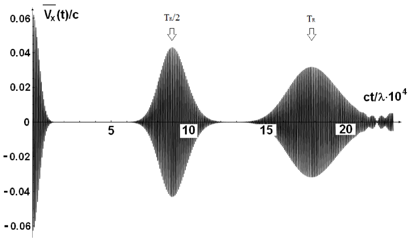
Figure 1: The dependence of the average velocity $\overline{v_{x}}(t)$ versus time for the initial wave packet, Eq.(24), with $\alpha=\beta$ and the parameters $\lambda/a=0.1$, $qa=5$ (that correspond to the value $n=n_{0}\approx 13$ and dispersion $\triangle n\sim\sqrt{n_{0}}\approx 3.5$).

If $n_{0}$ is large enough, the quantum interference of the wave packet components leads to the different types of periodicity. In Fig.1 we plot the dependence of $\overline{v_{x}}(t)$ for a relativistic wave packet with $qa=5$, $\alpha=\beta$, placed in the magnetic field $B\simeq 4.5\cdot 10^{7}$T. (Note that this magnetic field is 1.5 times greater than the maximum value achieved currently in laboratory experiments). In this case $\varphi_{n+1}-\varphi_{n}\approx\varphi^{\prime}_{n_{0}}+(\varphi^{\prime\prime}_{n_{0}}/2)(2n-2n_{0}+1)$. So, in the beginning the average velocity of the wave packet center oscillates with classical cyclotron motion period

$$T_{cl}=\frac{2\pi\hbar}{mc^{2}\varphi^{\prime}_{n_{0}}}=\frac{2\pi\varphi_{n_{0}}}{\omega_{c}},\;\omega_{c}=\frac{eBc}{\varepsilon_{n_{0}}}.$$

At large times $t>T_{D}$ these oscillations fade away but then appear again. The damping time $T_{D}$ can be estimated from Eq.(A4). For $|\varphi^{\prime\prime}_{n_{0}}|\tau\ll 1$ the amplitude of the oscillations is proportional to $\exp(-(qa\varphi^{\prime\prime}_{n_{0}}\tau/2)^{2})=\exp(-t^{2}/T_{D}^{2})$, where

$$T_{D}=\frac{2\lambda}{qac|\varphi^{\prime\prime}_{n_{0}}|}=\frac{2\hbar}{qa|\varepsilon^{\prime\prime}_{n_{0}}|}.$$

At times $T_{D}<t<T_{R}/2$ the average velocity components as well as average coordinates of the packet center are negligible. At $t\sim T_{R}/2$ (see Fig.1) the velocity oscillations will occur again. Here $T_{R}$ is the revival time at which the wave packet is fully reformed.A1 At $t_{k}=kT_{R}$ where $k$ is integer, the nonlinear (quadratic) term in the expansion of $\varphi_{n}$ has no effect, so that

$$T_{R}=\frac{4\pi\lambda}{c|\varphi^{\prime\prime}_{n_{0}}|}=\frac{4\pi\hbar}{|\varepsilon^{\prime\prime}_{n_{0}}|}.$$

Note that according to Averbukh and Perel’manA1 the moment $T_{R}/2$ is the first reconstruction time of the wave packet (see more detailed discussion below). For the considered wave packet Eqs.(29) and (30) give $T_{R}/T_{D}\sim 30$ that is in a good agreement with numerical calculations (Fig.1).

Now we describe some peculiarities of the space-time dynamics of the electron wave packet (24). Performing the integration over $p$ in Eq.(24), one has

$$\halign{\hbox to\displaywidth{$\hfil\displaystyle#\hfil$}\cr 0.0pt{\hfil$\displaystyle\psi({\bf r},t)=\frac{M(\rho,\theta)}{\sqrt{\alpha^{2}+\beta^{2}}}\sum_{n=0}\bigg{[}\frac{\gamma^{n-1}}{(n-1)!}(1-\delta_{n,0})e^{i\theta}\Big{(}\alpha d_{n},0,\frac{\beta b_{n}qa}{\sqrt{2n}},-\frac{\alpha b_{n}\rho}{\sqrt{2n}}e^{-i\theta}\Big{)}^{T}+\cr 0.0pt{\hfil$\displaystyle\hfill\frac{\gamma^{n}}{n!}\beta d_{n}(0,1,0,0)^{T}\bigg{]}e^{-i\theta n-i\varphi_{n}ct/\lambda}.\hfill\hbox to0.0pt{\hss(31)}\cr}}}$$

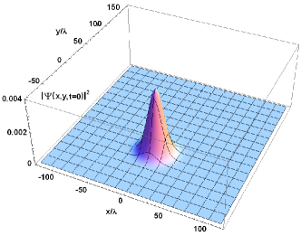
(a) (b)

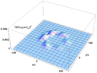
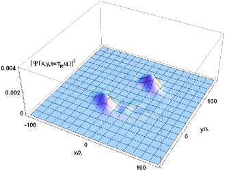
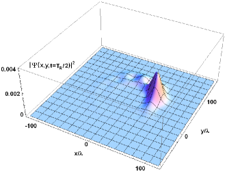
(c) (d) (e)

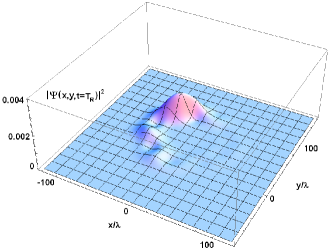
Figure 2: (Color online) The probability densities for the wave packet, Eq.(24), with $\alpha=\beta$ and the parameters $\lambda/a=0.1$, $qa=5$ at times: (a) $t=0$, (b) $t\approx T_{D}$, (c) $t\approx T_{R}/4$, (d) $t\approx T_{R}/2$, (e) $t\approx T_{R}$.

The details of the calculation are presented in the Appendix B. Here we use the notations

$$\frac{x}{a}=\rho\sin\theta,\,\frac{y-qa^{2}}{a}=\rho\cos\theta,\,\gamma=-\frac{qa\rho}{2},$$

$$M(\rho,\theta)=\frac{\exp\Big{(}-\frac{\rho^{2}+(qa)^{2}}{4}+\frac{i\rho\sin\theta(\rho\cos\theta+2qa)}{2}\Big{)}}{a\sqrt{2\pi}}.$$

In Fig.2 we plot the time evolution of the probability density $|\psi({\bf r},t)|^{2}$ calculated with the use of Eqs.(31), (32) and (33).

At the initial stage $t\ll T_{D}$ the motion of the wave packet is determined by the linear term of the expansion (A2). In this approximation

$$\psi({\bf r},t)=\psi_{cl}({\bf r},t),$$

where $\psi_{cl}({\bf r},t)$ is determined by Eq.(B4). As was noted above in our case the value $2n_{0}(\lambda/a)^{2}\simeq(q\lambda)^{2}=0.25$ so that $\psi_{cl}({\bf r},t)$ differs slightly from the coherent wave function of non-relativistic electron (see Eq.(B4)). Therefore, the shape of the wave packet $|\psi_{cl}({\bf r},t)|^{2}$ remains unchanged during its cyclotron motion, Eq.(B6), with the classical period $T_{cl}$ of the order of attoseconds ($10^{-18}s.$).

However, after a few orbits at $t\sim T_{D}$ (Fig.2b) the quadratic term in the expansion (A2) becomes significant, that leads to the dephasing of different terms in the superposition Eq.(31). As a result, the wave packet is decomposed in a host of sub-packets. As was shown by Averbukh and Perel’manA1 at time $t\approx mT_{R}/n$, where $m$ and $n$ are integer and $m/n$ is an irreducible fraction, the number of such sub-packets is equal to $N=n(3-(-1)^{n})/4$. The first reconstruction of wave packet takes place around time $t_{1}=T_{R}/2$A1 where the revival time $T_{R}$ is determined by Eq.(30) and $T_{R}\approx 2.3\cdot 10^{-16}\,s$ in our case. At that time $t_{1}$ the $n-$th term in the superposition (31) acquires the phase factor $f_{k}=e^{i\pi k^{2}}=e^{i\pi k}$, $k=n-n_{0}$, that leads to the result for the wave packet function (see Fig.2d)

$$\psi({\bf r},t_{1})=\psi_{cl}\Big{(}{\bf r},t_{1}+\frac{T_{cl}}{2}\Big{)}.$$

It should be noted in accordance with Eq.(B7) that the position of the reconstructed packet at the moments $T_{R}/2$ and $T_{R}$ does not coincide with initial position of the packet at $t=0$. At early times, for example, at $t_{2}=T_{R}/4$, the original wave packet splits into two subpackets (the fractional revival). In fact, the additional phase factor in this case $f_{k}=e^{i\pi k^{2}/2}$ is a periodic function $f_{k}=f_{k+2}$, so one can use the ordinary Fourier expansionA1

$$f_{k}=p_{0}+p_{1}e^{i\pi k},\,k=0,1,$$

from which

$$p_{0}=\frac{e^{i\pi/4}}{\sqrt{2}},\,p_{1}=\frac{e^{-i\pi/4}}{\sqrt{2}}.$$

Then, by substituting Eqs.(36) and (37) into Eq.(33) we obtain

$$\psi({\bf r},t_{2}=T_{R}/4)=\frac{e^{i\pi/4}}{\sqrt{2}}\psi_{cl}({\bf r},t_{2})+\frac{e^{-i\pi/4}}{\sqrt{2}}\psi_{cl}({\bf r},t_{2}+T_{cl}/2).$$

Note that according to Eqs.(B7) and (38), the angular distance between these two packets is $180^{\circ}$ (Fig.2c). Similar structure consisting of $N$ sub-packets evenly distributed along the classical orbit arises at the other fractional revival times. It should be noted, however, that the effects of fractional revivals are not manifested in the dependence of the mean velocity on the time (see Fig.1). The shape of the wave packet at revival time $T_{R}$ (Fig.2e) differs from the initial one (Fig.2a). The spreading of the packet at $t=T_{R}$ is connected with the next (cubic) term in the Taylor series.

Features of quantum dynamics of the relativistic wave packets described above should be seen in the nature of electromagnetic radiation emitted by the moving electrons. The radiation field as well as its intensity are determined by the multipole moments of system. Thus, at the initial stage of the evolution of wave packet ($t<T_{D}$), the dipole radiation with a frequency $\omega=\omega_{c}=\frac{eBc}{\varepsilon_{n_{0}}}$ is dominated. Its intensity (in the classical approach) is proportional to the square of the second time derivative of the average dipole moment $\ddot{\overline{\bf d}}(t)=-e\dot{\overline{\bf v}}(t)$, where the components of average velocity are determined by Eq. (25). At times $T_{D}<t<T_{R}/2$ the mean velocity of the packet is negligible (Fig.1). During this time electromagnetic emission is determined by both the time-dependent components of the quadrupole moment tensor $\overline{D_{\alpha,\beta}}=\int|\Psi({\bf r},t)|^{2}(3x_{\alpha}x_{\beta}-{\bf r}^{2}\delta_{\alpha,\beta})d{\bf r}$, and the magnetic moment $\overline{\bf m}=\frac{1}{2c}\int\Psi({\bf r},t)^{\dagger}[{\bf r},\hat{{\bf v}}]\Psi({\bf r},t)d{\bf r}$, where the wave function $\Psi({\bf r},t)$ is determined be the Eqs. (31)-(33). In particular, at the time moment $t=T_{R}/4$, when the initial wave packet splits into two sub-packets, the quadrupole radiation at the doubled frequency $2\omega_{c}$ is dominated, that is confirmed by numerical calculations of radiation intensity along $\bf n$ direction: $dI/d\Omega=\frac{1}{144\pi c^{5}}[\overline{\dddot{{\bf D}}},{\bf n}]^{2}$. In the time interval $\triangle t\sim 2T_{D}$ near the moment $t\sim T_{R}/2$ (see Fig.1) the dipole radiation begins to dominate again. Then at large times the multipole and magnetic-dipole terms become significant, and so on.

III.2 Spin dynamics

Below we describe and visualize the spin dynamics of the electron wave packet, Eq.(24), in the presence of a magnetic field ${\bf B}=(0,0,B)$. It is well-known that in non-relativistic quantum mechanics the electron spin precesses in the $(x,y)$-plane with cyclotron frequency $\omega=eB/mc$, so that the $S_{z}$-component remains constant. The spin operators $\hat{\bf S}$ for the Dirac particle

$$\hat{S}_{i}=\frac{\hbar}{2}{\Sigma_{i}}=\frac{\hbar}{2}\pmatrix{\sigma_{i}&0\cr 0&\sigma_{i}\cr},\qquad i=1,2,3.$$

do not commute with the Dirac Hamiltonian, Eq.(1). It follows that besides the usual spin precession which is more complicated in the relativistic case, the $S_{z}$-component changes with time in general. However, the average value of component $S_{z}$ is conserved for the wave packet consisting of the states with $E_{n}>0$ or $E_{n}<0$ only. It directly follows from the fact the commutator $[\hat{S}_{z},\hat{H}]$ is equal to zero in the subspace of the eigenvectors of the Dirac Hamiltonian for the same sign of energy. The original wave packet (Eq.(24)) satisfies this condition. Thus, we are interested to find the time-dependent average values of $\overline{S_{x}}(t)$ and $\overline{S_{y}}(t)$

$$\overline{S_{x,y}}(t)=\frac{\hbar}{2}\int\,d{\bf r}\psi^{\dagger}({\bf r},t)\Sigma_{x,y}\psi({\bf r},t),$$

where $\psi({\bf r},t)$ is given by Eq.(24). It is convenient to represent the result of calculations in the complex form

$$\halign{\hbox to\displaywidth{$\hfil\displaystyle#\hfil$}\cr 0.0pt{\hfil$\displaystyle\overline{\Sigma_{x}}(t)+i\overline{\Sigma_{y}}(t)=\frac{\alpha\beta}{\alpha^{2}+\beta^{2}}e^{-(qa)^{2}/2}\sum_{n=0}\frac{((qa)^{2}/2)^{n}}{n!}\times\cr 0.0pt{\hfil$\displaystyle\hfill\bigg{(}\sqrt{\frac{(\varphi_{n}+1)(\varphi_{n+1}+1)}{\varphi_{n}\varphi_{n+1}}}+\sqrt{\frac{n(\varphi_{n}-1)(\varphi_{n+1}-1)}{(n+1)\varphi_{n}\varphi_{n+1}}}\bigg{)}e^{ict(\varphi_{n+1}-\varphi_{n})/\lambda}.\hfill\hbox to0.0pt{\hss(41)}\cr}}}$$

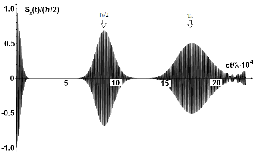
Figure 3: Time dependence $\overline{S_{x}}(t)$ for electron wave packet, Eq.(24), with the parameters $\lambda/a=0.1$, $qa=5$.

The dependence $\overline{S_{x}}(t)$ represented in Fig.3 is similar to the behavior of the average velocity component $\overline{v_{x}}(t)$ (see Fig.1). Thus, we arrive at the conclusion that the usual precession continues during several periods $T_{cl}$ only. At time $t\lesssim T_{D}$ the spin-rotation stops and arises again later at $t\lesssim T_{R}/2$. Note that the spin precession of a moving electron in a uniform magnetic field is closely connected to the conservation of helicity $\Sigma_{i}\cdot({\bf p}+e{\bf A}/c)_{i}$. Notice also that, as it follows from Eq.(41), the average values of spin components $\overline{\Sigma_{x}}=\overline{\Sigma_{y}}=0$ if the electron wave packet is a superposition of the states with $\lambda_{k}=1$ (or $\lambda_{k}=-1$) only (see Sec.I).

Now we consider the spin densities which we denote as $<S_{x,y}({\bf r},t)>=\frac{\hbar}{2}<\Sigma_{x,y}({\bf r},t)>$, where

$$<\Sigma_{x,y}({\bf r},t)>=\psi^{\dagger}({\bf r},t)\Sigma_{x,y}\psi({\bf r},t).$$

Using the expression for the wave function, Eq.(24), we find from Eq.(42) $<\Sigma_{x}({\bf r},t)>$ and $<\Sigma_{y}({\bf r},t)>$ as the real and imaginary parts of

$$\halign{\hbox to\displaywidth{$\hfil\displaystyle#\hfil$}\cr 0.0pt{\hfil$\displaystyle<\Sigma_{x}(\rho,\theta,t)>+i<\Sigma_{y}(\rho,\theta,t)>=\frac{\alpha\beta e^{-((qa)^{2}+\rho^{2})/2}}{2\pi a^{2}(\alpha^{2}+\beta^{2})}\sum_{m,n=0}\frac{(-qa\rho/2)^{n+m}}{n!m!}\times\cr 0.0pt{\hfil$\displaystyle\hfill\bigg{(}\sqrt{\frac{(\varphi_{m+1}+1)(\varphi_{n}+1)}{\varphi_{n}\varphi_{m+1}}}+\sqrt{\frac{n(\varphi_{n}-1)(\varphi_{m+1}-1)}{(m+1)\varphi_{n}\varphi_{m+1}}}\bigg{)}\times\hfill\cr 0.0pt{\hfil$\displaystyle\hfill\exp(ict(\varphi_{m+1}-\varphi_{n})/\lambda+i\theta(m-n)).\hfill\hbox to0.0pt{\hss(43)}\cr}}}}$$

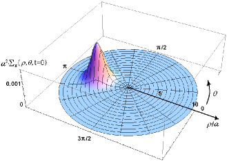
(a) (b)

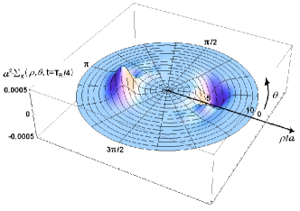
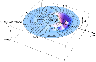
(c) (d)

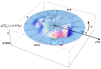
Figure 4: (Color online) The distribution of spin density $<\Sigma_{x}(\rho,\theta,t)>$ for the wave packet, Eq.(24), with the parameters $\lambda/a=0.1$, $qa=5$ at times: (a) $t=0$, (b) $t\approx T_{R}/4$, (c) $t\approx T_{R}/2$, (d) $t\approx T_{R}$.

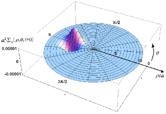
(a) (b)

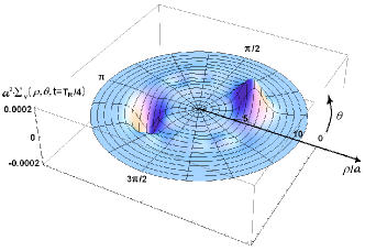
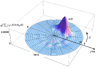
(c) (d)

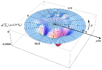
Figure 5: (Color online) The distribution of spin density $<\Sigma_{y}(\rho,\theta,t)>$ for the wave packet, Eq.(24), with the parameters $\lambda/a=0.1$, $qa=5$ at times: (a) $t=0$, (b) $t\approx T_{R}/4$, (c) $t\approx T_{R}/2$, (d) $t\approx T_{R}$.

Fig.4 and Fig.5 illustrate the distributions of $<\Sigma_{x}(\rho,\theta,t)>$ and $<\Sigma_{y}(\rho,\theta,t)>$ at the same moments as an Fig.2, i.e. $t=0,\,T_{R}/4,\,T_{R}/2,\,T_{R}$. Just as for electron probability density at $t\lesssim T_{R}$ in a main approximation the space-time evolution of the spin density is determined by the wave function $\psi_{cl}({\bf r},t)$, Eq.(B4), which corresponds to the ”classical” motion of the electron. So that let us define the functions ($\alpha=\beta$)

$$\halign{\hbox to\displaywidth{$\hfil\displaystyle#\hfil$}\cr 0.0pt{\hfil$\displaystyle<\Sigma_{x}^{cl}(\rho,\theta,t)>=\exp\Big{(}-\frac{\rho^{2}+(qa)^{2}+2\rho qa\cos(\theta+2\pi t/T_{c})}{2}\Big{)}\times\cr 0.0pt{\hfil$\displaystyle\hfill\Big{(}\cos\frac{2\pi t}{T_{c}}-\frac{\lambda^{2}}{4a^{2}}(qa\rho)\cos\theta\Big{)}/(2\pi a^{2}),\hfill\hbox to0.0pt{\hss(44)}\cr}}}$$

$$\halign{\hbox to\displaywidth{$\hfil\displaystyle#\hfil$}\cr 0.0pt{\hfil$\displaystyle<\Sigma_{y}^{cl}(\rho,\theta,t)>=\exp\Big{(}-\frac{\rho^{2}+(qa)^{2}+2\rho qa\cos(\theta+2\pi t/T_{c})}{2}\Big{)}\times\cr 0.0pt{\hfil$\displaystyle\hfill\Big{(}\sin\frac{2\pi t}{T_{c}}+\frac{\lambda^{2}}{4a^{2}}(qa\rho)\sin\theta\Big{)}/(2\pi a^{2}).\hfill\hbox to0.0pt{\hss(45)}\cr}}}$$

One can see from these expressions that at $t=0$ the $x$-component of spin density as a function of an angular variable $\theta$ has a maximum at $\theta_{0}=\pi$ (Fig.4a). The maximum and minimum values of the function $<\Sigma_{y}(\rho,\theta,0)>$ are in the vicinity of this point and differ in sign (see Fig.5a). At $t_{2}=T_{R}/4$, as was shown above, we have two ”classical” wave packets, Eq.(38), Fig.2c. Correspondingly,

$$<\Sigma_{x,y}(\rho,\theta,t_{2})>=\frac{1}{2}(<\Sigma_{x,y}^{cl}(\rho,\theta,t_{2})>+<\Sigma_{x,y}^{cl}(\rho,\theta,t_{2}+T_{cl}/2)>),$$

that is illustrated by Fig.4b and Fig.5b. Note that such simple summation in Eq.(46) is only valid if the width of each of the wave packets is less than the cyclotron orbit length.

IV Space-time dynamics of the mesoscopic wave packets formed by the positive and negative energy eigenstates

In this Section we investigate the relativistic dynamics of the wave packet containing both the positive and negative energy states with $\lambda_{k}=1$. Correspondingly we restrict ourselves to the wave states with two nonzero components $\{\psi_{1},\psi_{4}\}$. As was noted in Section II the temporal dynamics of such states is governed by the part of Dirac Hamiltonian which is identical to a Jaynes-Cummings interaction. Besides of the general peculiarities of quantum dynamics of the system with the nonlinear energy spectrum (collapse and revival phenomenon), the existence of two energy bands leads to another effect – Zitterbewegung (ZB). This phenomenon, generating a highly oscillatory motion, is caused by the interference between positive and negative energy components of the wave packet. We will consider here the effect of ZB on the evolution of the electron velocity as well as on the spin polarization.

Let at the time $t=0$ the initial wave packet is given by

$$\psi({\bf r},0)=\psi_{c}({\bf r})\pmatrix{|\uparrow>\cr 0\cr},$$

where

$$\psi_{c}({\bf r})=\frac{1}{a\sqrt{2\pi}}\exp\Big{(}-\frac{x^{2}+y^{2}}{4a^{2}}+iqx+\frac{ixy}{2a^{2}}\Big{)}$$

is the wave function of coherent state, which can be written in the form

$$\psi_{c}({\bf r})=\int dp\,\varphi_{p}(x)g(p)\sum_{n=0}c_{n+1}\phi_{n}(y-y_{c}).$$

The coefficients $g(p)$ and $c_{n}$ in this expression are determined by Eqs.(22) and (23). Using Eqs.(20), (47) and (49), one can obtain

$$\halign{\hbox to\displaywidth{$\hfil\displaystyle#\hfil$}\cr 0.0pt{\hfil$\displaystyle\psi({\bf r},\tau)=\int dp\,\varphi_{p}(x)g(p)\times\cr 0.0pt{\hfil$\displaystyle\hfill\sum_{n=1}\bigg{[}d_{n}\pmatrix{d_{n}\phi_{n-1}(y-y_{c})|\uparrow>\cr-b_{n}\phi_{n}(y-y_{c})|\downarrow>\cr}\exp(-i\varphi_{n}\tau)+b_{n}\pmatrix{b_{n}\phi_{n-1}(y-y_{c})|\uparrow>\cr d_{n}\phi_{n}(y-y_{c})|\downarrow>\cr}\exp(i\varphi_{n}\tau)\bigg{]}.\hfill\hbox to0.0pt{\hss(50)}\cr}}}$$

Performing integration over $p$ (see Appendix B, Eq.(B3)), we get finally

$$\psi({\bf r},\tau)=\Psi_{1}({\bf r},\tau)\pmatrix{|\uparrow>\cr 0\cr}+\Psi_{2}({\bf r},\tau)\pmatrix{0\cr|\downarrow>\cr},$$

where

$$\Psi_{1}({\bf r},\tau)=\psi_{c}({\bf r})\exp\Big{(}-\frac{q}{2}(qa^{2}-y+ix)\Big{)}\sum_{n=1}\frac{(q(qa^{2}-y+ix))^{n-1}}{2^{n-1}(n-1)!}\Big{(}\cos(\varphi_{n}\tau)-\frac{i\sin(\varphi_{n}\tau)}{\varphi_{n}}\Big{)},$$

$$\Psi_{2}({\bf r},\tau)=-\psi_{c}({\bf r})\exp\Big{(}-\frac{q}{2}(qa^{2}-y+ix)\Big{)}\sum_{n=1}\frac{(q(qa^{2}-y+ix))^{n-1}}{2^{n-1}(n-1)!}\frac{i\lambda\sin(\varphi_{n}\tau)}{a^{2}\varphi_{n}}(qa^{2}-y+ix).$$

As above, first of all we calculate the average velocity of the packet center

$$\overline{v_{i}}(t)=c\int\psi^{\dagger}\hat{\sigma}_{i}\psi\,d{\bf r}.$$

Substituting the expressions for the components of the wave function Eqs.(52), and (53) into Eq.(54) after the integration over the $x$, $y$ coordinates we have

$$\overline{v_{x}}(\tau)=c\frac{\lambda}{a}\exp\Big{(}-(qa)^{2}/2\Big{)}\sum_{n=1}\frac{(qa)^{2n-1}}{2^{n-1}(n-1)!\varphi_{n}\varphi_{n+1}}\Big{(}\cos((\varphi_{n+1}-\varphi_{n})\tau)-\cos((\varphi_{n+1}+\varphi_{n})\tau)\Big{)},$$

$$\overline{v_{y}}(\tau)=c\frac{\lambda}{a}\exp\Big{(}-(qa)^{2}/2\Big{)}\sum_{n=1}\frac{(qa)^{2n-1}}{2^{n-1}(n-1)!\varphi_{n}}\Big{(}\sin((\varphi_{n+1}-\varphi_{n})\tau)-\sin((\varphi_{n+1}+\varphi_{n})\tau)\Big{)}.$$

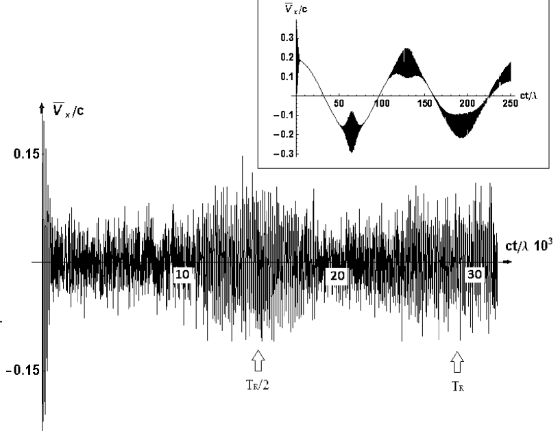
Figure 6: The dependence of the average velocity $\overline{v_{x}}(t)$ versus time for the initial wave packet, Eq.(47), with the parameters $\lambda/a=0.5$, $qa=10$. The oscillations of the average velocity $\overline{v_{x}}(t)$ at times $t\geq T_{cl}$ are shown in the insert.

Note that these equations depend on not only on the energy difference $\varphi_{n+1}-\varphi_{n}$ as in Eq.(25), but on the sum $\varphi_{n+1}+\varphi_{n}$ also. The last dependence leads to the high frequency of the ZB oscillations. The dependence of the average velocity $\overline{v_{x}}(\tau)$ on time for the packets parameters $\lambda/a=0.5,\,qa=10$ (that corresponds to the dominant value of $n=n_{0}\simeq 50$) is shown in Fig.6. Like the case of the wave packet discussed in Section II, the behavior of this function is accompanied by the collapse and revival phenomenon. For the parameters of our wave packet the corresponding periods of cyclotron motion and revivals are $T_{cl}\approx 126\lambda/c$ and $T_{R}\approx 26660\lambda/c$. In addition, the insert in Fig.6 clearly demonstrates the ZB oscillations with peculiar frequency $\omega_{ZB}=2\varphi_{n_{0}}c/\lambda=10.2c/\lambda\simeq 7.85\cdot 10^{21}\,s^{-1}$. Besides, these oscillations occur in short intervals near time moments $t_{k}=kT_{cl}/2\,(k=1,2,\ldots)$, that is connected with the feature of the space-time evolution of the wave packet probability density. At $t>0$ the initial wave packet (Fig.7a) splits into two parts (Fig.7b) with the amplitudes which are slightly different. These sub-packets containing the states of one sign of the energy rotate with cyclotron frequency in the opposite directions and meet each other every one-half of the cyclotron period (see Fig.7c, 7d). The duration of ZB-oscillations is determined by the relation of the packets size to their relative velocity. Note that in the moment of time $t=T_{cl}/4$ the spin parts of the sub-wave packets with $E_{n}>0$ and $E_{n}<0$ differ slightly. Thus, the spatial part of the full wave function (50) is a linear superposition of the mesoscopic states (see Appendix C). At $t\sim t_{k}$ the parts with positive and negative energy have significant overlap in the coordinate space. This is a necessary condition for the existence of Zitterbewegung (see insert in Fig.6).

At times $t\sim T_{cl}$ the effect of the quadratic term in the Taylor expansion of the energy, Eq.(A2), is insignificant. For times much greater than the cyclotron period the dephasing appears in individual terms in Eq.(50) due to the term $(n-n_{0})^{2}$, that leads to the collapse of the sub-wave packets. At intermediate times $T_{cl}\ll t_{n}\leq T_{R}$, where $t_{n}\approx mT_{R}/n$ ($m/n$ is irreducible fraction), the fractional revival of each sub-packets occurs. As a result, each sub-packet is decomposed into $N=n(3-(-1^{n}))/4$ packets-fractions. Particularly, at $t=T_{R}$ each of the two sub-packets (with positive or negative energy) restores at various points on the cyclotron orbit, that makes it impossible reshaping of the initial wave packet entirely. At time $T_{R}/4$ we should see four packets-fractions. However, this result is not consistent with the distribution of the probability density shown in Fig.8a due to the significant influence of the term $\sim(n-n_{0})^{3}$ in the series (A2) for times $t\leq T_{R}$. This statement is illustrated in Fig.8b, which shows at time $t=T_{R}/4$ the probability density, taking into account the first three terms in the expansion (A2) only.

Consider now the average value of the spin operator. Since the initial state of the wave packet, Eq.(47), belongs to one of the invariant subspaces (with $\lambda_{k}=1$), the average spin projections $\overline{S_{x}}=\overline{S_{y}}=0$. Using the definition $\overline{S_{z}}=(\hbar/2)\hat{\sigma}_{z}$ and Eqs.(51), (52), and (53) we obtain

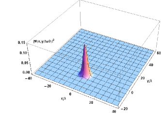
(a) (b)

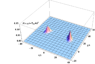
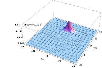
(c) (d)

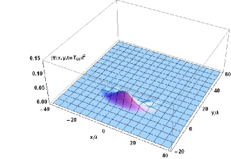
Figure 7: (Color online) The distribution of the electron probability density for initial wave packet, Eq.(47), with the parameters $\lambda/a=0.5$, $qa=10$: (a) $t=0$, (b) $t\approx T_{cl}/4$, (c) $t\approx T_{cl}/2$, (d) $t\approx T_{cl}$.

$$\overline{S_{z}}(\tau)=\frac{\hbar}{2}\sum_{n=1}|c_{n}|^{2}\bigg{(}\frac{1+2n(\lambda/a)^{2}\cos(2\varphi_{n}\tau)}{\varphi_{n}^{2}}\bigg{)},$$

where the coefficients $c_{n}$ are determined by Eq.(23). Corresponding dependence is shown in Fig.9. It is clearly seen that the average value of the $z$-component of spin oscillates with the ZB-frequency $\omega_{ZB}\approx 2\varphi_{n_{0}}c/\lambda$ and is accompanied by the phenomenon of collapse and revival. In this case unlike the previous definition, Eq.(30), the corresponding revival time is determined by the cyclotron period $T_{rev}=T_{cl}/2$.Berm ; Gea In intervals between the ZB-oscillations the average value of $\overline{S_{z}}(t)$ is not equal to zero. As mentioned above, the space-time evolution of the original wave packet (47) is described by the part of the Dirac Hamiltonian, Eq.(1) that is identical to the Jaynes-Cummings model in quantum optics.JC So one can conclude that Eq.(56) is similar to the well-known expression for the population of the ground state of two-level atom exposed to the action of the classical electromagnetic fieldA1 .

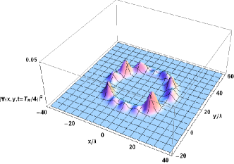
(a) (b)

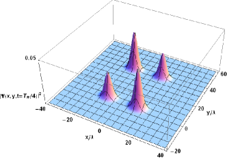
Figure 8: (Color online) Electron probability density for initial wave packet, Eq.(47), at $qa=10$, $\lambda/a=0.5$, $t\approx T_{R}/4$: (a) for real energy spectrum, (b) for the spectrum obtained by taking into account the first three terms in the expansion (A2) only.

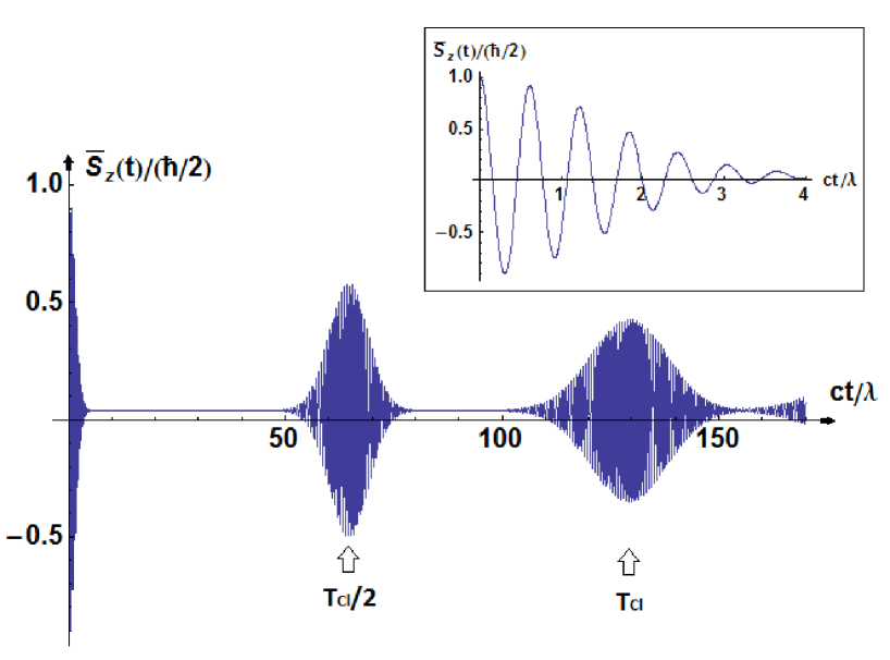
Figure 9: (Color online) The time dependence of average spin $\overline{S_{z}}$ (in units of $\hbar/2$) for initial wave packet, Eq.(47), for $qa=10$, $\lambda/a=0.5$. The oscillations of the average spin at short times $t\ll T_{cl}$ are shown in the insert.

V Summary

In this work we have analyzed the cyclotron dynamics of relativistic wave packets, moving in external constant magnetic field over cyclotron orbit. The components of electron wave function were calculated (see Eqs. (31), (52), and (53)), as well as, average velocities of the packet $\overline{v_{x}}(t)$. It was shown that for the case when the wave packet consists of positive energy states only the effects of collapse and revival of electron and spin densities can be observed.

On short-time $t\leq T_{cl}$ (where $T_{cl}$ is the cyclotron period) the coherent wave packet rotates with the classical frequency over the cyclotron orbit. We analyzed the complex evolution of spin densities and average spin components. The precession of spin densities one can see in Fig.4, Fig.5. We visualized $N$ packets-fractions which form at times of fractional revivals $t=mT_{R}/n$ ($N=n(3-(-1)^{n})/4$, as was shown by Averbukh and Perel’manA1 ). In our opinion, the dynamics of such structures can be studied experimentally by investigating the nature of electromagnetic multipole radiation and absorption. It was found that the effects of fractional revivals can not be observed via time-dependence of average velocity.

We compared the dynamics of wave packet described above with the behavior of the wave packet containing the states with both the positive and negative energies (Sec.IV). In the last case the splitting of the initial wave packet takes place at $t<T_{cl}$. These two sub-packets rotate with the cyclotron frequency in opposite directions and meet each other every one-half of the cyclotron period that results in the high-frequency ZB oscillations. It was shown (see Appendix C) that of time $t=T_{rev}/2=T_{cl}/4$ the electron spin and orbital degrees of freedom become disentangled. In this case spin states play the role of the internal states of the atom that has or has not radioactively decayed and the orbital states correspond to the cat in the original Schrödinger modelSh . At $t=T_{R}$ each of the two sub-packets restores at different points of the cyclotron orbit. So that the full reshaping of initial wave packet is impossible unlike the case of wave packet including the positive energy states only.

VI Acknowledgments

The authors are grateful to M.A. Martin-Delgado, who drew their attention to the problem of ”Dirac cat”, discussed in Ref.Berm . This work was supported by a program of the Russian Ministry of Education and Science ”The development of scientific potential of higher education” (Project No. 2.1.1/10910), and Russian Foundation for Basic Research (Grant No. 11-02-00960a).

Appendix A

In this Appendix we find the approximate expression for the average electron velocity for the packet parameters $qa\gg 1$ and $\lambda/a\ll 1$ (we consider $qa\simeq 5,\,\lambda/a\simeq 0.1$). Corresponding wave function (20) represents the quantum superposition of the states sharply peaked around large enough central value $n=n_{0}$. In fact, for $(qa)^{2}/2\gg 1$ the Poisson distribution $|c_{n}|^{2}$ (see Eq.(23)) can be replaced by Gaussian one

$$e^{-(qa)^{2}/2}\frac{\Big{(}\frac{(qa)^{2}}{2}\Big{)}^{n}}{n!}\approx\frac{1}{\sqrt{2\pi n_{0}}}exp\bigg{(}-\frac{(n-n_{0})^{2}}{2n_{0}}\bigg{)},$$

where $n_{0}\simeq(qa)^{2}/2\simeq 12$ and dispersion $\bigtriangleup n\simeq\sqrt{n}_{0}$. So, we expand the dimensionless energy spectrum $\varphi_{n}$ as a power series in $(n-n_{0})$, restricting ourselves to the quadratic termsA1 ; Rom

$$\varphi_{n}=\varphi_{n_{0}}+\varphi^{\prime}_{n_{0}}(n-n_{0})+\frac{\varphi^{\prime\prime}_{n_{0}}}{2}(n-n_{0})^{2}.$$

For the given values of the packet parameters $\varphi_{n}$ is close to $1$ and the coefficients before the exponents in Eq.(25) can be estimated, in good approximation, as

$$\sqrt{\frac{\varphi_{n+1}-1}{2(n+1)\varphi_{n+1}}}\simeq\frac{\lambda/a}{\sqrt{2}},\;\sqrt{\frac{\varphi_{n}+1}{\varphi_{n}}}\simeq\sqrt{2},$$

that allows us to carry out the sum over $n$ in Eq.(25). The result is

$$\halign{\hbox to\displaywidth{$\hfil\displaystyle#\hfil$}\cr 0.0pt{\hfil$\displaystyle\overline{v_{x}}(\tau)=\frac{\hbar q}{m}\exp\bigg{(}-\Big{(}qa\sin\frac{\varphi^{\prime\prime}_{n_{0}}\tau}{2}\Big{)}^{2}\bigg{)}\times\cr 0.0pt{\hfil$\displaystyle\hfill\cos\bigg{(}\frac{\varphi^{\prime\prime}_{n_{0}}\tau}{2}\bigg{)}\cos\bigg{(}\varphi^{\prime}_{n_{0}}\tau-\varphi^{\prime\prime}_{n_{0}}\Big{(}\frac{(qa)^{2}}{2}-1\Big{)}\tau+\frac{(qa)^{2}}{2}\sin\varphi^{\prime\prime}_{n_{0}}\tau\bigg{)},\hfill\hbox to0.0pt{\hss(A4)}\cr}}}$$

$$\halign{\hbox to\displaywidth{$\hfil\displaystyle#\hfil$}\cr 0.0pt{\hfil$\displaystyle\overline{v_{y}}(\tau)=\frac{\hbar q}{m}\exp\bigg{(}-\Big{(}qa\sin\frac{\varphi^{\prime\prime}_{n_{0}}\tau}{2}\Big{)}^{2}\bigg{)}\times\cr 0.0pt{\hfil$\displaystyle\hfill\cos\bigg{(}\frac{\varphi^{\prime\prime}_{n_{0}}\tau}{2}\bigg{)}\sin\bigg{(}\varphi^{\prime}_{n_{0}}\tau-\varphi^{\prime\prime}_{n_{0}}\Big{(}\frac{(qa)^{2}}{2}-1\Big{)}\tau+\frac{(qa)^{2}}{2}\sin\varphi^{\prime\prime}_{n_{0}}\tau\bigg{)}.\hfill\hbox to0.0pt{\hss(A5)}\cr}}}$$

As clearly seen from these expressions the velocity oscillations reduce exponentially with time. The corresponding damping time is determined by Eq.(29).

Appendix B

i) Below we find more detailed expression for wave function (24). In order to do that we perform the integration over $p$. The corresponding integral has the form

$$Q_{k}=\int\limits_{-\infty}^{+\infty}\varphi_{p}(x)g(p)\phi_{k}(y-y_{c}(p))\,dp,$$

where $\varphi_{p}(x)=(1/\sqrt{2\pi\hbar})\exp(ipx/\hbar)$, where $g(p)$ is determined by Eq.(22) and $\phi_{k}(y-y_{c}(p))$ is the well-known linear harmonic oscillator function. Putting these expressions into Eq.(B1) and using Gaussian transformation for Hermite polynomials $H_{k}(y)$RG

$$\frac{1}{\sqrt{\pi}}\int\limits_{-\infty}^{+\infty}e^{-(x-y)^{2}}H_{k}(y)\,dy=(2x)^{k},$$

we finally obtain

$$Q_{k}=\frac{((y-qa^{2}-ix)/a)^{k}}{\sqrt{2^{k+1}k!\pi a^{2}}}\exp\Big{(}\frac{2ix(y+qa^{2})-x^{2}-(y-qa^{2})^{2}}{4a^{2}}\Big{)}.$$

Substituting the above expression into Eq.(24) and using polar coordinates (32) one gets Eq.(31).

ii) Let us now calculate the electron wave function $\psi({\bf r},t)=\psi_{cl}({\bf r},t)$ at the short times $t\ll T_{D}$ when we can neglect the quadratic term in the expansion (A2). Then recollecting that for a given wave packet the coefficients $d_{n}$ and $b_{n}$ can be approximated by the expressions $d_{n}\simeq 1$ and $b_{n}\simeq\sqrt{n/2}\lambda/a$, we find after summation from Eq.(31)

$$\halign{\hbox to\displaywidth{$\hfil\displaystyle#\hfil$}\cr 0.0pt{\hfil$\displaystyle\psi_{cl}(\rho,\theta,t)=\frac{M(\rho,\theta)}{\sqrt{\alpha^{2}+\beta^{2}}}S\Big{(}\theta+\frac{2\pi t}{T_{cl}}\Big{)}\exp\Big{(}-i\Big{(}\frac{\varepsilon_{n_{0}}}{\hbar}+\frac{2\pi}{T_{cl}}(1-n_{0})\Big{)}t\Big{)}\times\cr 0.0pt{\hfil$\displaystyle\hfill\Big{(}\alpha,\beta e^{i\frac{2\pi t}{T_{cl}}},\frac{\beta q\lambda}{2},-\frac{\alpha\lambda\rho}{2a}e^{-i\theta}\Big{)}^{T},\hfill\hbox to0.0pt{\hss(B4)}\cr}}}$$

where

$$S(u)=\exp\Big{(}-\frac{qa\rho}{2}(\cos u-i\sin u)\Big{)}$$

and $M(\rho,\theta)$ is determined by Eq.(33). The solution (B4) describes the coherent weakly-relativistic wave packet propagating along the cyclotron orbit without changing its shape. In particular, at $\alpha=\beta$ the corresponding probability density has the Gaussian form

$$|\psi_{cl}(\rho,\theta,t)|^{2}=\frac{1+\frac{\lambda^{2}}{8a^{2}}(\rho^{2}+(qa)^{2})}{2\pi a^{2}}\exp\Big{(}-\frac{\rho^{2}+(qa)^{2}+2\rho qa\cos(\theta+2\pi t/T_{cl})}{2}\Big{)}.$$

It is clearly seen that the center of the wave packet corresponding to the angle

$$\theta_{c}=\pi-\frac{2\pi t}{T_{c}}$$

rotates with cyclotron frequency $\omega_{c}=2\pi/T_{c}$ similar to the motion of a classical electron placed in a magnetic field.

Appendix C

Below we show that the wave packet discussed in Sec.IV (Eqs.(47), (48)) at $t_{0}=T_{cl}/4$ is a coherent superposition of mesoscopic statesGea ; Berm . To do it we consider the time evolution of the initial state

$$\psi_{+}({\bf r},0)=\psi_{c}({\bf r})|+>,$$

where the ”orbital” wave function of the coherent state $\psi_{c}({\bf r})$ is given by Eq.(48) and the initial Dirac spinor $|+>$ has the form

$$|+>=d_{n_{0}}\pmatrix{|\uparrow>\cr 0\cr}+b_{n_{0}}\pmatrix{0\cr|\downarrow>\cr}$$

with the coefficients $d_{n_{0}}$ and $b_{n_{0}}$ are given by Eq.(14). Here as above we assume that the mean value of $n$ in Eq.(49) is large enough: $\overline{n}=(qa)^{2}/2=n_{0}\gg 1$.

The state (C1) evolves as

$$\halign{\hbox to\displaywidth{$\hfil\displaystyle#\hfil$}\cr 0.0pt{\hfil$\displaystyle\psi_{+}({\bf r},\tau)=\int dp\,\varphi_{p}(x)g(p)\Bigg{[}\sum_{n=1}c_{n}^{+}\pmatrix{d_{n}\phi_{n-1}(y-y_{c})|\uparrow>\cr-b_{n}\phi_{n}(y-y_{c})|\downarrow>\cr}e^{-i\varphi_{n}\tau}+\cr 0.0pt{\hfil$\displaystyle\hfill\sum_{n=0}c_{n}^{-}\pmatrix{b_{n}\phi_{n-1}(y-y_{c})|\uparrow>\cr d_{n}\phi_{n}(y-y_{c})|\downarrow>\cr}e^{i\varphi_{n}\tau}\Bigg{]},\hfill\hbox to0.0pt{\hss(C3)}\cr}}}$$

where the coefficients $c_{n}^{\pm}$ are

$$\halign{\hbox to\displaywidth{$\hfil\displaystyle#\hfil$}\cr 0.0pt{\hfil$\displaystyle c_{n}^{+}=c_{n}d_{n_{0}}d_{n}-c_{n+1}b_{n_{0}}b_{n},\cr 0.0pt{\hfil$\displaystyle\hfill c_{n}^{-}=c_{n}d_{n_{0}}b_{n}+c_{n+1}b_{n_{0}}b_{n}.\hfill\hbox to0.0pt{\hss(C4)}\cr}}}$$

Using the weak dependence on $n$ for the coefficients $d_{n}$ and $b_{n}$ and also using the expression for $c_{n}$, Eq.(23), we obtain from (C4) at $n\simeq n_{0}\gg 1$

$$c_{n}^{+}=c_{n},\quad c_{n}^{-}=0.$$

Then it is not difficult to show that

$$\psi_{+}({\bf r},\tau)=\bigg{(}e^{-i\varphi^{\prime}_{n_{0}}\tau}d_{n_{0}}\pmatrix{|\uparrow>\cr 0\cr}+b_{n_{0}}\pmatrix{0\cr|\downarrow>\cr}\bigg{)}\psi_{c+}({\bf r},\tau),$$

where

$$\psi_{c+}({\bf r},\tau)=\int dp\,\varphi_{p}(x)g(p)\sum_{n=0}c_{n+1}\phi_{n}(y-y_{c})e^{-i\varphi_{n}\tau}.$$

In the same way one can compute the evolution of the initial state

$$\psi_{-}({\bf r},0)=\psi_{c}({\bf r})|->,$$

$$|->=b_{n_{0}}\pmatrix{|\uparrow>\cr o\cr}-d_{n_{0}}\pmatrix{0\cr|\downarrow>},$$

$$\psi_{-}({\bf r},\tau)=\bigg{(}e^{i\varphi^{\prime}_{n_{0}}\tau}b_{n_{0}}\pmatrix{|\uparrow>\cr 0\cr}-d_{n_{0}}\pmatrix{0\cr|\downarrow>\cr}\bigg{)}\psi_{c-}({\bf r},\tau),$$

where $\psi_{c-}({\bf r},\tau)$ is determined by Eq.(C7) in which $\exp(-i\varphi_{n}\tau)$ should be replaced by $\exp(i\varphi_{n}\tau)$. Note that the initial spin functions are orthogonal: $<+|->=0$.

Thus, the initial wave packet, Eq.(47), can be represented as a superposition

$$\psi_{c}({\bf r})\pmatrix{|\uparrow>\cr 0\cr}=d_{n_{0}}\psi_{+}({\bf r},0)+b_{n_{0}}\psi{-}({\bf r},0),$$

so that

$$\psi({\bf r},\tau)=d_{n_{0}}\psi_{+}({\bf r},\tau)+b_{n_{0}}\psi_{-}({\bf r},\tau)$$

describing two sub-packets which at $t<T_{cl}=(2\pi/\varphi^{\prime}_{n_{0}})\lambda/c$ rotate counterclockwise $(\psi_{+}({\bf r},\tau))$ and clockwise $(\psi_{-}({\bf r},\tau))$ in the $xy-$plane. At the moment of time $t_{0}=T_{cl}/4$ as follows from Eqs.(C6) and (C10)

$$\bigg{|}<+|->\Big{|}_{t=t_{0}}\bigg{|}=\sqrt{\frac{2n_{0}(\lambda/a)^{2}}{1+2n_{0}(\lambda/a)^{2}}}\approx 0.98$$

for $n_{0}=50$ and $\lambda/a=0.5$, and we conclude that the spin parts of wave functions $\psi_{\pm}({\bf r},t)$ differ slightly. That means that ”orbital” part of full wave function (C12) at that time is a linear superposition of the mesoscopic states $\psi_{c+}({\bf r},t_{0})$ and $\psi_{c-}({\bf r},t_{0})$ (the so-called ”Schrödinger cat”). The corresponding probability density $|\psi({\bf r},t_{0}=T_{cl}/4)|^{2}$ is shown in Fig.7b. The generation of coherent superposition of mesoscopic states for the Dirac particle placed in the magnetic field was predicted in Ref.Berm .

References

- (1) I.Sh.Averbukh and N.F.Perel’man, Sov. Phys. Usp. 34, 572 (1991).
- (2) J.Parker and S.R.Stroud,Jr., Phys. Rev. Lett. 56, 716 (1986).
- (3) Z.Dacic and C.R.Stroud,Jr., Phys. Rev. A 42, 6308 (1990).
- (4) E.Romera and F. de los Santos, Phys. Rev. B 80, 165416 (2009).
- (5) J.J.Torres and E.Romera, Phys. Rev. B 82, 155419 (2010).
- (6) A.Bermudes, M.A.Martin-Delgado, and R. Solano, Phys. Rev. Lett. 99, 123602 (2007).
- (7) E.T.Jaynes and F.W.Cummings, Proc. IEEE 51, 89 (1963).
- (8) T.M.Rusin and W.Zawadzki, Phys. Rev. D 82, 125031 (2010).
- (9) E.Schrödinger, Naturwissenschaften 23, 807812 (1935); 23, 823828 (1935); 23, 844849 (1935).
- (10) P.Krekora, Q.Su, and R.Grobe, Phys. Rev. Lett. 93, 043004 (2004).
- (11) R.Gerritsma, G.Kirchmair, F.Zahringer, E.Solano, R.Blatt, and C.F.Roos, Nature 463, 68 (2010).
- (12) J.Gea-Banacloche, Phys. Rev. A 44, 5913 (1991).
- (13) A.Auffeves et al., Phys. Rev. Lett. 91, 230405 (2003).
- (14) J.A.Yeazell et al., Phys. Rev. Lett. 64 (1990).
- (15) M.J.J.Vrakking, D.M.Villeneuve, and A.Stolow, Phys. Rev. A. 54, R37 (1996).
- (16) I.Sh.Averbukh, M.J.J.Vrakking, D.M.Villeneuve, and A.Stolow, Phys. Rev. Lett. 77, 3518 (1996).
- (17) C. Monroe, D. Meekhof, B. King, and D. Wineland, Science 272, 1131 (1996).
- (18) V.Ya.Demikhovskii, G.M.Maksimova, A.A.Perov, and E.V.Frolova, Phys. Rev. A 82, 052115 (2010).
- (19) V.Ya.Demikhovskii, G.M.Maksimova, and E.V.Frolova, Phys. Rev. B 78, 115401 (2008); V.Ya.Demikhovskii, G.M.Maksimova, and E.V.Frolova, Phys. Rev. B 81, 115206 (2010).
- (20) G.M.Maksimova, V.Ya.Demikhovskii, and E.V.Frolova, Phys. Rev. B 78, 235321 (2008).
- (21) I.S.Gradshteyn and I.M.Ryzhik, Tables of Integrals, Series and Products Academic, New York (1980).