Genesis of the dusty Universe: modeling submillimetre source counts

Abstract

We model the evolution of infrared galaxies using a phenomenological approach to match the observed source counts at different infrared wavelengths. In order to do that, we introduce a new algorithm for reproducing source counts which is based on direct integration of probability distributions rather than using Monte-Carlo sampling. We also construct a simple model for the evolution of the luminosity function and the colour distribution of infrared galaxies which utilizes a minimum number of free parameters; we analyze how each of these parameters is constrained by observational data. The model is based on pure luminosity evolution, adopts the Dale & Helou Spectral Energy Distribution (SED) templates, allowing for evolution in the infrared luminosity-colour relation, but does not consider Active Galactic Nuclei as a separately evolving population. We find that the $850\,\mu$m source counts and redshift distribution depend strongly on the shape of the luminosity evolution function, but only weakly on the details of the SEDs. Based on this observation, we derive the best-fit evolutionary model using the $850\,\mu$m counts and redshift distribution as constraints. Because of the strong negative $K$-correction combined with the strong luminosity evolution, the fit has considerable sensitivity to the sub-$L_{*}$ population at high redshift, and our best-fit shows a flattening of the faint end of the luminosity function towards high redshifts. Furthermore, our best-fit model requires a colour evolution which implies the typical dust temperatures of objects with the same luminosities to decrease with redshift. We then compare our best-fit model to observed source counts at shorter and longer wavelengths which indicates our model reproduces the $70\,\mu$m and $1100\,\mu$m source counts remarkably well, but under-produces the counts at intermediate wavelengths. Analysis reveals that the discrepancy arises at low redshifts, indicating that revision of the adopted SED library towards lower dust temperatures (at a fixed infrared luminosity) is required. This modification is equivalent to a population of cold galaxies existing at low redshifts, as also indicated by recent Herschel results, which are underrepresented in IRAS sample. We show that the modified model successfully reproduces the source counts in a wide range of IR and submm wavelengths.

1 Introduction

Although dust is an unimportant component in the mass budget of galaxies, its presence radically alters the emergent spectrum of star forming galaxies. Since stars are born in dusty clouds, most of the energy of young stars is absorbed by dust particles, which are heated by the absorption process and radiate their energy away by thermal emission at infrared (IR) and submillimetre (submm) wavelengths. As a result, the infrared radiation of star forming galaxies is a useful measure of the massive star formation rate. Mainly due to the atmospheric opacity, the thermal radiation from dust could not be systematically studied until the launch of IRAS in the mid-1980s, which provided the first comprehensive view of the nearby dusty Universe. Ten years later COBE discovered the Cosmic Infrared Background (CIB) (Puget et al., 1996; Fixsen et al., 1998) and it turned out the observed power of the CIB is comparable to what can be deduced from the optical Universe. This was in contrast to the observations of local galaxies which suggest only one third of the energy output of galaxies is in IR bands (Lagache et al., 2005). Moreover, the relatively flat slope of the CIB at long wavelengths indicated a population of dusty galaxies which are distributed over a wide range of redshifts (Gispert et al., 2000). Thanks to various large surveys performed with different satellites and ground based observatories, this background radiation is now partly resolved into point sources at different wavelengths. While at shorter wavelengths the emission is mainly coming from local and low redshift galaxies, longer wavelengths contain information about larger distances.

The shape of emission spectrum of warm dust particles resembles a modified blackbody spectrum with a peak varying with the typical dust temperature which is observed to be around $T\sim 30-40$K in galaxies; therefore the far-IR (FIR) and submm spectrum of a typical dusty galaxy consists of a peak at rest-frame wavelengths around $\lambda\sim 100-200\mu m$ which drops on both sides (see Figure 1). While the presence of other emitters like polycyclic aromatic hydrocarbons (PAHS) and Active Galactic Nuclei (AGNs) complicates the shape of spectra at shorter wavelengths, at submm wavelengths the spectra behave like modified blackbodies and their amplitudes drop steeply. In fact, because of this steep falloff in the Rayleigh-Jeans tail of the Spectral Energy Distribution (SED), the observed flux density at a fixed submm wavelength can rise by moving the SED in redshift space (the so called $K$-correction), which counteracts the cosmological dimming. It turns out that the interplay between these two processes enables us to observe galaxies at submm wavelengths out to very high redshifts (see also the discussion in Section 5 and Figure 7).

After the first observations of SCUBA at $850\,\mu$m confirmed the importance of submm galaxies at high redshifts (Smail et al., 1997), there were many subsequent surveys using different instruments which explored different cosmological fields (Smail et al., 2002; Webb et al., 2003; Borys et al., 2003; Greve et al., 2004; Coppin et al., 2006; Bertoldi et al., 2007; Austermann et al., 2010; Scott et al., 2010; Vieira et al., 2010) and also some surveys which used gravitational lensing techniques to extend the observable submm Universe to sub-mJy fluxes (Smail et al., 1997; Chapman et al., 2002; Knudsen et al., 2008; Johansson et al., 2011).

While low angular resolution makes individual identifications and spectroscopy a daunting task, the surface density of sources as a function of brightness (i.e., the source counts) can be readily analysed and contains significant information about the population properties and their evolution. One can assume simple smooth parametrized models for the evolution of dusty galaxies and relate their low redshift observed properties (e.g., the total IR luminosity function, which we simply call the luminosity function, or in short LF hereafter) to their source counts (Blain & Longair, 1993; Guiderdoni et al., 1997; Blain et al., 1999; Chary & Elbaz, 2001; Rowan-Robinson, 2001; Dole et al., 2003; Lagache et al., 2004; Lewis et al., 2005; Le Borgne et al., 2009; Valiante et al., 2009). Such backward evolution models usually combine SED templates and the low redshift properties of IR galaxies which are allowed to change with redshift based on an assumed parametric form, together with Monte-Carlo techniques to reproduce the observed source counts. These models are therefore purely phenomenological, and suppress the underlying physics. Their power lies exclusively in providing a parametrized description of statistical properties of the galaxy population under study, and the evolution of these properties. The results of such modeling provides a description of the constraints that must be satisfied (in a statistical sense) and could be explored further by more physically motivated models such as hydrodynamical simulations embedded in a $\Lambda$CDM cosmology, with subgrid prescriptions for star formation and feedback (e.g. Schaye et al. (2010)). It is important to realize that backward evolution models are constrained only over limited observational parameter space (e.g., at particular observing wavelengths, flux levels, redshift intervals, etc.), and are ignorant of the laws of physics. Therefore it is dangerous to use them outside of their established validity ranges; in other words, these models have descriptive power but little explanatory power. As a result, one of the most instructive uses of these models is in analyzing where they fail to reproduce the observations, and how they can be modified to correct for these failures which implies that the underlying assumptions must be revised. This is the approach that we use in the present paper.

Since nowadays many and various observational constraints exist (e.g. source counts at various IR and submm wavelengths, colour distributions, redshift distribution), backward evolution models can reach considerable levels of sophistication. However, early backward evolution models used only a few SED templates (or sometimes even only one SED) to represent the whole population of dusty galaxies. This approach neglects the fact that dusty galaxies are not identical and span a variety of dust temperatures and hence SED shapes. As a result, such models cannot probe the possible evolution in the SED properties of submm galaxies, for which increasing observational support has been found during the last few years (Chapman et al., 2005; Pope et al., 2006; Chapin et al., 2009; Symeonidis et al., 2009; Seymour et al., 2010; Hwang et al., 2010).

In addition, existing backward evolution models typically use only “luminosity” and/or “density” evolution which respectively evolves the characteristic luminosity (i.e., $L_{\star}$) and the amplitude of the LF without changing its shape. In other words, they do not consider any evolution in the shape of the luminosity function. Finally, the intrinsically slow Monte-Carlo methods used in many of the models make the search of parameter space for the best-fit model laborious and tedious.

In this paper, we use a new and fast algorithm which is different from conventional Monte-Carlo based algorithms, for calculating the source counts for a given backward evolution model. We also use a complete library of IR SED templates which form a representative sample of observed galaxies, at least at low redshifts. This will enable us to address questions about the evolution of colour distribution of dusty galaxies during the history of the Universe. We also consider a new evolution form for the LF which allows us to constrain evolution in the shape of the LF in addition to quantifying its amplitude changes.

The structure of the paper is as follows: in §2 we present different ingredients of our parametric colour-luminosity function (CLF) evolution model and introduce a new algorithm for the fast calculation of the source counts for a given CLF. Then, after choosing our observational constraints for $850\,\mu$m objects in §3 we try to find a model consistent with those constraints by studying the sensitivity of the produced source counts to different parameters in §4. After finding a $850\,\mu$m-constrained best-fit model, we test its performance in producing source counts at other wavelengths in §5 which leads us to a model capable of producing source counts in a wide range of IR and submm wavelengths. Finally, after discussing the astrophysical implications of our best-fit model in §6, we end the paper with concluding remarks. Throughout this paper, we use the standard $\Lambda$CDM cosmology with the parameters $\Omega_{\rm{m}}=0.3$, $\Omega_{\rm{\Lambda}}=0.7$ and $h=0.75$.

2 Model ingredients

Although luminosity is the main parameter to differentiate between different galaxies, it is an integrated property of SED and cannot distinguish between different SED shapes corresponding to different physical processes taking place in different objects with similar outgoing integrated energy fluxes. Using colour indicators can resolve this degeneracy. Dale et al. (2001) demonstrated that the $R(60,100)$ which is defined as $\log(S_{60\,\mu\rm{m}}/S_{100\,\mu\rm{m}})$, is the best single parameter characterization of IRAS galaxies. Moreover, it was shown that IRAS galaxies exhibit a slowly varying correlation between $R(60,100)$ and luminosity such that objects with larger characteristic luminosities have warmer characteristic colours (Dale et al., 2001; Chapman et al., 2005; Chapin et al., 2009). Based on these facts, we construct a model for the Colour-Luminosity Function (hereafter CLF). This model consists of the observed CLF in the local Universe and a parametric evolution function. Then, by adopting a suitable set of SED models, we calculate the source count of IR objects at different wavelengths and compare the results with observations.

2.1 CLF at $z=0$

The local volume density of IRAS galaxies, $\Phi_{0}(L,C)$, can be parametrized as a function of total IR luminosity, $L$, and $R(60,100)$ colour, $C$, where the total infrared luminosity is calculated by integrating over the SED from $3$ to $1100\,\mu$m (Dale et al., 2001). Furthermore, it is possible to express the local colour-luminosity distribution as the product of the local luminosity function, $\Phi_{0}(L)$, and the local conditional probability of a galaxy having the colour $C$ given the luminosity $L$, $P_{0}(C|L)$,

$$\Phi_{0}(L,C)=\Phi_{0}(L)P_{0}(C|L).$$ (1)

Since the IRAS galaxies represent an almost complete sample of IR galaxies out to the redshift $\sim 0.1$ (Saunders et al., 1990), we use the luminosity and colour functions found by analyzing a flux limited sample of $S_{60\,\mu{\rm{m}}}>1.2{\rm{Jy}}$ IRAS galaxies (Chapman et al., 2003; Chapin et al., 2009). Chapman et al. (2003) and Chapin et al. (2009) analyze this sample which covers most of the sky, using an accessible volume technique for finding the LF and fit a dual power law function to the observed luminosity distribution. The parametric form of luminosity function based on Chapin et al. (2009) is given by

$$\Phi_{0}(L)=\rho_{*}(\frac{L}{L_{*}})^{1-\alpha}(1+\frac{L}{L_{*}})^{-\beta},$$ (2)

where ${L}_{*}=5.14\times 10^{10}{L}_{\odot}$ is the characteristic knee luminosity, $\rho_{*}=1.22\times 10^{-14}{\rm{Mpc}}^{-3}L_{\odot}^{-1}$ is the number density normalization of the function at $L_{*}$, and $\alpha=2.59$ and $\beta=2.65$ characterize the power-laws at the faint ($L<L_{*}$) and bright ($L>L_{*}$) ends, respectively.

Chapman et al. (2003) and Chapin et al. (2009) also found a Gaussian representation for the colour distribution of IRAS galaxies

$$P_{0}(C\mid L)=\frac{1}{\sqrt{2\pi}\sigma_{\rm{c}}}\exp[-\frac{1}{2}\times(\frac{C-C_{0}}{\sigma_{\rm{c}}})^{2}],$$ (3)

where $C_{0}$ can be represented by a dual power law function

$$C_{0}=C_{*}-\delta\log(1+\frac{L^{\prime}}{L})+\gamma\log(1+\frac{L}{L^{\prime}}),$$ (4)

with $C_{*}=-0.48$, $\delta=-0.06$, $\gamma=0.21$ and $L^{\prime}=3.2\times 10^{9}L_{\odot}$, and the distribution width, $\sigma_{\rm{c}}$, is expressed as

$$\sigma_{\rm{c}}=\sigma_{\rm{f}}(1-2^{-L^{\prime}/L})+\sigma_{\rm{b}}(1-2^{-L/L^{\prime}}),$$ (5)

where $\sigma_{\rm{f}}=0.2$ and $\sigma_{\rm{b}}=0.128$ (Chapin et al., 2009).

2.2 CLF evolution

The CLF introduced in the previous section, contains information about the distribution of IR galaxies only in the nearby Universe. For modeling the IR Universe at higher redshifts, its evolution must be modeled. The necessity of the CLF evolution with redshift is shown directly by the fact that the observed power of the the CIB is comparable to what can be deduced from the optical cosmic background cannot be explained by our understanding of the local Universe which indicates the infrared output of galaxies is only one third of their optical output (Lagache et al., 2005). Furthermore, several studies have shown for a fixed total IR luminosity the typical temperature of infrared sources is lower at higher redshifts (Chapman et al., 2005; Pope et al., 2006; Chapin et al., 2009; Symeonidis et al., 2009; Seymour et al., 2010; Hwang et al., 2010; Amblard et al., 2010), which advocates an IR colour evolution. Therefore, we need to adopt a reasonable form of evolution in the luminosity and colour distributions to reproduce correctly the CLF evolution of IR galaxies with redshift.

There are three different ways to evolve the local luminosity function of IR galaxies: (i) changing $\rho_{*}$ with redshift (i.e., density evolution); (ii) changing $L_{*}$ with redshift (i.e., luminosity evolution) and (iii) changing the bright and faint end slopes (i.e., $\alpha$ and $\beta$) with redshift. While the density and luminosity evolution change the abundances of all sources independent of their luminosities, they leave the shape of the LF unchanged. Such models are called translational models since they amount to only a translation of the LF in parameter space. Going beyond translational models, a variation of the shape of LF with redshift (i.e., varying $\alpha$ and $\beta$ slopes in equation 2) can be used to change the relative contributions of bright and faint sources at different redshifts.

As discussed by Blain et al. (1999), luminosity and density evolution affect the CIB predicted by the models similarly, but luminosity evolution has a much stronger effect on the source counts. Combining source counts and integrated background can therefore distinguish between luminosity and density evolution. The result of this analysis shows luminosity evolution must strongly dominate over density evolution, since pure density evolution consistent with the observed $850\,\mu$m source counts would overpredict the integrated background by a factor 50 to 100 (Blain et al., 1999). We therefore assume negligible density evolution. However, as we will show in Section 4, luminosity evolution is not sufficient to reproduce the correct source count and redshift distribution of submm galaxies, which forces us to drop the assumption of a purely translational LF evolution model. Moreover, there is no reason to assume that the slopes of LF at faint and bright ends remain the same at all redshifts. Therefore, we allow them to change in our model and introduce a redshift dependent LF which can be written as

$$\Phi(L,z)=\rho_{*}(\frac{L}{g(z)L_{*}})^{1-\alpha_{z}}(1+\frac{L}{g(z)L_{*}})^{-\beta_{z}},$$ (6)

which is similar to equation (2) but now $\alpha_{z}$ and $\beta_{z}$ are changing with redshift and $L_{*}$ is multiplied by $g(z)$, which we refer to as the luminosity evolution function.

Since the average total-IR-luminosity density and its associated star formation density closely follow the luminosity evolution function, we choose a form of luminosity evolution which is similar to the observed evolution of the cosmic star formation history (see Hopkins & Beacon (2006)); in other words, we assume that the luminosity evolution is a function which is increasing at low redshifts and after reaching its maximum turns into a decreasing function of look-back time at high redshifts:

$$g(z)=\left\{\begin{array}[]{lll}(1+z)^{n}&\mbox{ if }z\leq z_{a}\\ (1+z_{a})^{n}&\mbox{ if }z_{a}<z\leq z_{b}\\ (1+z_{a})^{n}(1+z-z_{b})^{m}&\mbox{ if }z_{b}<z\end{array}\right.$$ (7)

where $n$, $m$, $z_{a}$ and $z_{b}$ are constants. As we will show in Section 4.2, the source count is not strongly sensitive to the model properties at high redshifts. In other words, the sensitivity of the source count calculation to the difference between $z_{a}$ and $z_{b}$ is much less than its high sensitivity to the value of $z_{a}$ itself. Moreover, the model outputs are not highly sensitive to the slope of $g(z)$ at high redshifts if it remains negative (i.e., $m<0$). Therefore, we can simplify the model by assigning suitable fixed values to $z_{b}-z_{a}$ and $m$, without any significant change in its flexibility. We choose $z_{b}-z_{a}=1$ and $m=-1$, knowing that any different choice for those values can be compensated by a very small change in $z_{a}$ or/and $n$. we will discus this issue in more detail in Section 4.2.

We also adopt linear forms for changing $\alpha_{z}$ and $\beta_{z}$ with redshift

$$\alpha_{z}=2.59+a_{\alpha}z,$$ (8)

$$\beta_{z}=2.65+a_{\beta}z,$$ (9)

where $a_{\alpha}$ and $a_{\beta}$ are constants. We apply the slope evolution only for $z<\frac{z_{a}+z_{b}}{2}$ noting that the observed source count is not very sensitive to the exact properties of our model at very high redshifts and extending the evolution of LF slopes to even higher redshifts does not change our results.

As mentioned earlier, some studies have shown that high redshift IR galaxies have lower dust temperatures than low redshift galaxies, at a fixed total IR luminosity. In our model, in order to evolve the colour distribution accordingly, we adopt a relation similar to Valiante et al. (2009) to shift the centre of the colour distribution for a given luminosity towards colours associated with lower dust temperatures (i.e., smaller $R(60,100)$ values) at higher redshifts (see Figure 11). In this way, the colour distribution of IR galaxies can be written as

$$P(C\mid L)=\frac{1}{\sqrt{2\pi}\sigma_{\rm{c}}}\exp[-\frac{1}{2}\times(\frac{C-C^{\prime}_{0}}{\sigma_{\rm{c}}})^{2}],$$ (10)

where $\sigma_{\rm{c}}$ is given by equation (5) and $C^{\prime}_{0}$ is

$$C^{\prime}_{0}=C_{*}-\delta\log(1+\frac{L^{\prime}(1+z)^{w}}{L})+\gamma\log(1+\frac{L}{L^{\prime}(1+z)^{w}}),$$ (11)

where $w$ is a constant. Although for colour evolution we adopt a similar formalism to Valiante et al. (2009), unlike them we allow $w$ to vary as a free parameter which enables us to constrain the colour evolution as well.

Based on the above formalism, the general CLF of IR galaxies can be written as

$$\Phi(L,C,z)=\Phi(L,z)P(C|L),$$ (12)

where $\Phi(L,z)$ and $P(C|L)$ are defined by equations (6)-(11).

2.3 SED Model

Figure 1: Some SED samples from the template library of Dale & Helou (2002) which we use in our model. The blue, green, orange and red lines (from top to bottom) are respectively associated with colours $C=0.16$, $0.04$, $-0.27$ and $-0.54$. The normalization is arbitrary.

Several studies have shown that AGNs do not dominate the FIR energy output of the Universe (Swinbank et al., 2004; Alexander et al., 2005; Chapman et al., 2005; Lutz et al., 2005; Valiante et al., 2007; Pope et al., 2008; Menendez-Delmestre et al., 2009; Fadda et al., 2010; Jauzac et al., 2010). Therefore, in order to avoid unnecessary complexity in our model we adopt a single population of galaxies, modeled with only one family of SEDs representing star forming galaxies.

This choice is justified for long wavelengths, for instance at $850\,\mu$m, by considering the fact that at those wavelengths the AGN contribution to the observed flux is negligible. In other words, to be able to change the $850\,\mu$m fluxes and source counts, AGN should be the dominant contributor to the SED at rest-frame wavelengths longer than $\sim 200\,\mu$m which is highly unlikely.

On the other hand, excluding AGN contribution could be potentially important at shorter wavelengths: if we adopt a simple assumption where the AGN continuum is well represented by a simple torus model (Efstathiou et al., 1995; Valiante et al., 2009), then a strong enough AGN could create a bump, on top of the starburst SED, at rest-frame wavelength ranges $\sim 10-50\,\mu$m (see Figure 2 in Efstathiou et al. (1995) and Figure 9 in Valiante et al. (2009)). This feature, together with increasing AGN luminosity with redshift could modify the observed source counts at observed wavelengths shorter than $200\,\mu$m but still is unlikely to affect submm counts.

However, Mullaney et al. (2011) recently used the deepest available Herschel survey and showed that for a sample of X-ray selected AGNs up to $z\sim 3$, the observed $100\,\mu$m and $160\,\mu$m fluxes are not contaminated by AGN. Consequently, even if all the galaxies which contribute to the FIR and submm source counts host AGN, their observed fluxes is driven by star formation activity at wavelengths around $100\,\mu$m or longer.

In order to get accurate SED templates for star-forming galaxies, we use the Dale et al. (2001) and Dale & Helou (2002) SED models which are produced by a semi-empirical method to represent spectral energy distribution of star-forming galaxies in the IR region of spectrum. Dale et al. (2001) add up emission profiles of different dust families (i.e. large grains, very small grains and polycyclic aromatic hydrocarbons) which are exposed to a range of radiation field strengths in a parametrized form to generate the SED of different star-forming systems. In this way, it is possible to produce the SED corresponding to each $R(60,100)$ colour and scale it to the desired total infrared luminosity. In our model, we use spectral templates taken from the Dale & Helou (2002) catalog which provides 64 normalized SEDs with different $R(60,100)$ colours, ranging from $-0.54$ to $0.21$. Some SED examples taken from this template set are illustrated in Figure 1.

2.4 The algorithm

Given the distribution of objects in the Universe, and their associated SEDs, it is possible to calculate the number of sources which have observed fluxes above some detection threshold, $S_{\rm{th}}$, at a given wavelength $\lambda=\lambda_{\rm{obs}}$:

$$N(>S_{\rm{th}})=\int\int\int Q\times\Phi(L,C,z)\frac{dV}{dz}dzdLdC,$$ (13)

where $V$ is the volume and $Q$ is the probability that a source with luminosity $L$, colour $C$ and redshift $z$ has an observed flux density greater than $S_{th}$ at that wavelength (i.e., its detection probability). At each point of redshift-colour-luminosity space, $Q$ is either $1$ or $0$ for any particular galaxy, but it is useful to think of $Q$ as the average probability of detection for galaxies in each cell of that space.

In order to calculate $Q$, we first note that for each source with a given luminosity, $L$, and colour, $C$, there is a redshift, $z_{\rm{max}}$, at which the observed flux is equal to the detection threshold

$$S(L,C,\lambda_{0},z_{\rm{max}})=S_{\rm{th}}=\frac{(1+z_{\rm{max}})L_{\nu}(L,C,\lambda_{0})}{4\pi D_{L}^{2}(z_{\rm{max}})},$$ (14)

where $D_{L}$ is the luminosity distance and $L_{\nu}$ is the rest-frame luminosity density ($\rm{W\,Hz}^{-1}$) of the object with total luminosity $L$ and colour $C$ at wavelength $\lambda_{0}=\lambda_{\rm{obs}}/(z+1)$.

Now consider a cell defined by redshift interval $\Delta z=z_{2}-z_{1}$ (where $z_{1}<z_{2}$), luminosity interval $\Delta L=L_{2}-L_{1}$ and colour interval $\Delta C=C_{2}-C_{1}$. Assuming negligible colour and luminosity evolution between $z_{1}$ and $z_{2}$, the average detection probability in the cell is equal to the fraction of detectable objects in that cell which is:

$$Q=\left\{\begin{array}[]{lll}1&\mbox{ if }z_{\rm{max}}>z_{2}\\ \frac{D^{3}(z_{\rm{max}})-D^{3}(z_{1})}{D^{3}(z_{2})-D^{3}(z_{1})}&\mbox{ if }z_{1}\leq z_{\rm{max}}\leq z_{2}\\ 0&\mbox{ if }z_{\rm{max}}<z_{1}\end{array}\right.$$ (15)

where $D(z)$ is the proper distance equivalent to redshift $z$. For writing equation 15, we assumed galaxies to be distributed uniformly in space between redshifts $z_{1}$ and $z_{2}$. Consequently, based on equation 13, the number of objects which are contributing to the source count in each cell of the redshift-colour-luminosity space is

$$\Delta N(>S_{\rm{th}})=Q\times\bar{\Phi}(L,C,z)\Delta L\Delta C\Delta V,$$ (16)

where $\Delta V$ is the volume corresponding to the redshift interval $\Delta z$ and $\bar{\Phi}(L,C,z)$ is the average CLF in the cell, which for small enough $\Delta L$, $\Delta C$ and $\Delta z$ can be written as

$$\bar{\Phi}(L,C,z)=\Phi(\bar{L},\bar{C},\bar{z}).$$ (17)

Then, the total source count is obtained by summing over the contribution from all cells (see Appendix A).

As a result of using $Q$ and its special form as expressed in equation 15, our algorithm computes the source count for continuously distributed sources in the Universe, independent of the size of $\Delta z$ which is used in equation 13. Thanks to this property, the computational cost required for the source count calculation is reduced significantly, and the small size of $\Delta z$ is only necessary for accurate calculation of $K$-corrected SEDs and CLFs at different redshifts and not to guarantee a uniform distribution of sources (see also Appendix A).

Now that we have all the tools ready, we can test the capability of our model in reproducing the observed properties of $850\,\mu$m sources and find which particular choices of model parameters are implied. In the following sections, we first discuss the observational constraints that we want to reproduce with our model and then we will proceed with finding the best-fit model which can reproduce those properties.

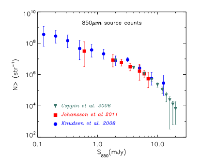
Figure 2: A compilation of some observed $850\,\mu$m source counts. Blue circles, green triangles and red squares are respectively data points taken from Knudsen et al. (2008), Coppin et al. (2006) and Johansson et al. (2011).

3 $850\,\mu$m Observational Constraints

3.1 Observed $850\,\mu$m source count

Among several existing extragalactic submm surveys which provide source counts at $850\,\mu$m (Coppin et al., 2006; Weiss et al., 2009; Austermann et al., 2010), the SCUBA Half-Degree Extragalactic Survey (SHADES) (Coppin et al., 2006) is the largest one which has the most complete and unbiased sample. However, this survey and other surveys which use JCMT and the same blank field method are restricted by the JCMT confusion limit of $\sim 2$mJy at $850\,\mu$m and cannot probe the source counts of the fainter population. Using a complementary method, the lensing technique has been used to probe $850\,\mu$m source counts to flux thresholds as low as $0.1$mJy (Smail et al., 2002; Knudsen et al., 2008; Johansson et al., 2011). As we will show later in this section, the sensitivity of bright and faint submm source counts to the evolution of dusty galaxies is completely different and it is essential to incorporate a large dynamic range to constrain possible evolutionary scenarios. Therefore, we use the best available observational information at both faint and bright tails of $850\,\mu$m source count, by combining all of the SHADES data points with those of Knudsen et al. (2008) at flux thresholds $<2$mJy to assemble our reference source count which is also in agreement with other observations (see Figure 2).

3.2 Redshift distribution of bright $850\,\mu$m sources

Although the observed number counts at $850\,\mu$m, especially at faint fluxes, are sensitive to the redshift distribution of infrared galaxies, they do not constrain it directly. As we will discuss later, different models with different redshift distributions can reproduce the $850\,\mu$m source counts with the same accuracy. Therefore, it is important to impose an additional constraint on redshift distribution of those objects.

Unfortunately, studying the redshift distribution of submm galaxies is extremely difficult and there are only a few works on spectroscopically confirmed redshift distribution of bright submm galaxies with observed fluxes grater than $\sim 4-5$ mJy (Chapman et al., 2005; Wardlow et al., 2011). Those studies show a redshift distribution peaking around $z\sim 2$ (see the right panel in Figure 6). We use this redshift distribution as one of our observed constraints and force our model to reproduce a redshift distribution which peaks at the same redshift.

4 Finding $850\,\mu$m best-fit Model

In order to be able to extract meaningful trends and differentiate between them, it is important to keep our phenomenological model as simple as possible. It is therefore desirable to find the minimum number of free parameters without which the model cannot produce an acceptable result. Furthermore, the role of different parameters are not identical: while some parameters are not strongly constrained, small changes in others can change the result significantly. It is also important to look at degeneracies between various parameters; some parameters are not independent and varying one may be compensated by varying the others. In this section we investigate our model to understand those issues before presenting our best-fit model.

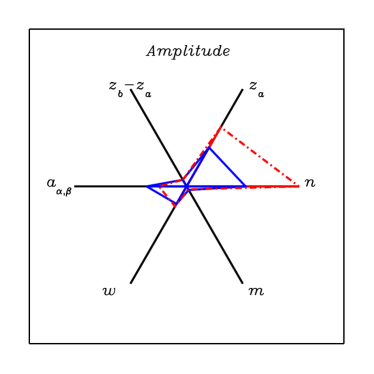
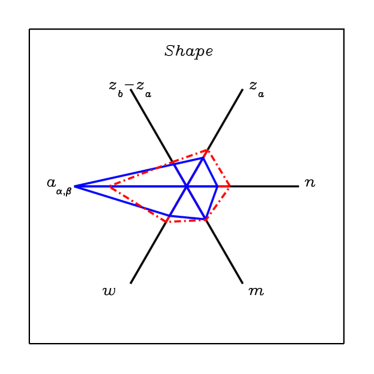
Figure 3: The sensitivity of the model to various parameters. While the left panel illustrates how much the variation of different parameters could change the amplitude of the $850\,\mu$m source count curve, the right panel shows their effect in changing the shape of the source count curve. To measure the amplitude changes, we varied each parameter by $10\%$ around its best-fit value and measured the difference in the total source counts. The shape sensitivity is probed by measuring the relative change each varying parameter can cause in the ratio between two source counts at faint and bright flux thresholds (i.e. $\frac{N_{1{\rm{mJy}}}}{N_{{\rm{1Jy}}}}$). The lengths of the coloured segments on each axis shows how large those changes are. The blue (red) segments which are connected by solid (dash-dotted) lines represent the result as we increased (decreased) the value of each parameter. We show parameters $a_{\alpha}$ and $a_{\beta}$ on one axis since their effect in changing the source count properties is similar.

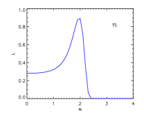
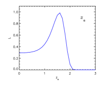
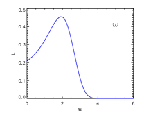
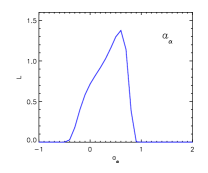
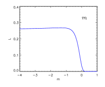
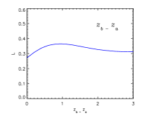
Figure 4: The likelihood (i.e. $exp(-\frac{1}{2}\chi^{2})$) distribution of different parameters for the best-fit model. For each panel, we fixed all the parameters at their best-fit values and changed only one parameter at a time. By varying each parameter, the quality of the fit and hence the likelihood is changing. We normalized the amplitude of curves such that the area under each curve (i.e. the total probability) be unity.

4.1 The source count curve: Amplitude vs. Shape

To match the observed source counts, our model should be able to reproduce both the typical number of sources (i.e., the amplitude of the source count curve as a function of flux threshold) and the ratio between the source counts at faint and bright flux thresholds (i.e., the shape of the source counts curve). Following this line of argument, we can categorize our model parameters into two different groups: those which play a stronger role in forming the amplitude of the curve and those which mainly affect its shape. As mentioned earlier, the luminosity evolution (see equation 7) has the dominant role in determining the amplitude of the source count curve while its shape is controlled by other ingredients of our model which are colour evolution and the evolution of LF slopes.

These trends are illustrated in Figure 3. In the left panel, the relative contribution of each parameter in changing the amplitude of the source count curve is visualized; the length of the coloured segments along each axis (coloured segments along different axis are connected to each other) represents the sensitivity of source count amplitude to that parameter. The length of coloured segments is computed by changing all the model parameters (one at a time) by the same fraction, for instance $10\%$, and measure the change caused in the total source count. The segments which are connected by dot-dashed (red) and solid (blue) lines correspond respectively to a decreasing and an increasing parameter. In the right panel, the relative contribution of different parameters in controlling the shape of the source counts curve is shown. In this figure, the length of coloured segments represents the change in the ratio between faint and bright source counts. This time, we measured how much the ratio between a very faint source count, like $1$ mJy, and a very bright one, like $1$ Jy, is changing due to a fixed change in different parameters (e.g., $10\%$). The dot-dashed (red) and solid (blue) lines connect the coloured segments which correspond to an increase or a decrease in the values of the parameters.

As is evident from these diagrams, the amplitude of the source count curve is strongly sensitive to the parameters of the luminosity evolution, particularly $z_{a}$ and $n$, while its shape is determined mainly by an evolution in the shape of LF and/or the strength of the colour evolution.

4.2 The luminosity evolution

The luminosity evolution is the backbone of our model and has the most important role in producing the observed source counts and the redshift distribution of $850\,\mu$m objects. However, it is not surprising that the calculated source count is not strongly sensitive to the model properties at high redshifts. This is mainly because objects at very high redshifts have decreasing fluxes (despite the advantageous $K$-correction). Consequently, the chosen value of $m$ has a negligible effect on the amplitude and shape of the source count curve (see Figure 3). Nevertheless, one should note that this argument would not necessarily work if the population of bright IR galaxies continued to evolve with look-back time for all redshifts. In other words, the exact value of $m$ is not strongly constrained by the observed source counts and all the negative values can produce similar results (see the middle panel in the bottom row of Figure 4).

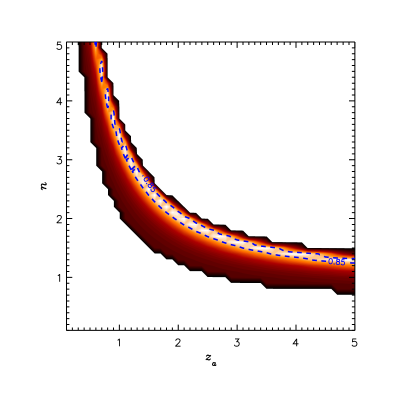
Figure 5: Map of likelihoods for models with different $n$ and $z_{a}$ where $[w,a_{\alpha},a_{\beta}]=[0,0,0]$. The region which contains the best-fit models is in the middle of the coloured band and surrounded by the dashed blue contours which indicate the likelihood of $0.85$.

Contrary to $m$, the source count curve is very sensitive to the exact values of $n$ and $z_{a}$ which respectively control the rate by which the characteristic luminosity of IR galaxies increases with redshift and up to which redshift this growth continues. However, there are two solutions for reproducing the same source counts: one is to increase the characteristic IR luminosity rapidly up to a relatively low redshift and the other one is to increase the characteristic IR luminosity by a moderate rate but for a longer period of time (i.e., up to higher redshifts). Therefore, as illustrated in Figure 5, there is a degeneracy between $n$ and $z_{a}$ and one cannot constrain them individually by looking at the observed source counts. However, additional information about the redshift distribution of submm galaxies or the slope by which the characteristic IR luminosity is growing at low redshifts could resolve this degeneracy. As we will discuss later, the former constraint is used in finding our best-fit model.

Unlike $n$ and $z_{a}$, the length of the redshift interval during which the luminosity evolution remains constant before starting to decline, $z_{b}-z_{a}$, is not an essential part of our model. We only introduced this feature to have a smoother transition between growing and declining characteristic IR luminosity and also redshift distribution of submm galaxies. As Figures 3 and 4 show, variations in the adopted value for $z_{b}-z_{a}$ do not change the source count significantly. Moreover, any change in its value could be compensated by a very small change in $n$ and/or $z_{a}$.

Based on these considerations and as we already mentioned in Section 2.2, we reduce the number of free parameters we use in our model by choosing $m=-1$ and $z_{b}-z_{a}=1$. Furthermore, the observed redshift distribution of submm galaxies which peaks around $z\sim 2$ (Chapman et al., 2005; Wardlow et al., 2011), limits the acceptable values of $z_{a}$ to $\sim 1.6$ (see the right panel in Figure 6).

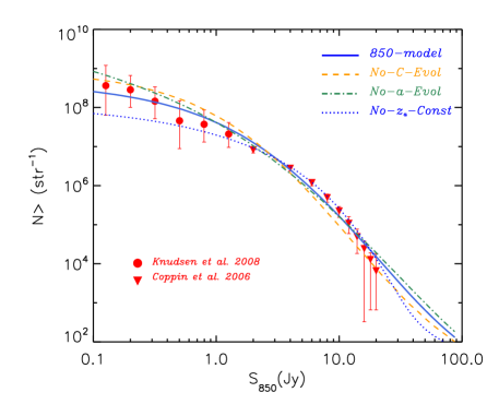
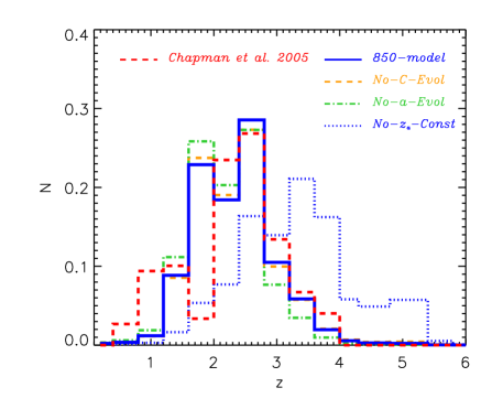
Figure 6: Left panel: The best-fit model which is constrained by $850\,\mu$m source count and the redshift distribution of submm galaxies (the blue solid line) is illustrated next to the reference observed data points (see Section 3). For comparison, three other best-fit models are also plotted: the best-fit model without colour evolution shown by the dashed orange line (i.e., “No-C-Evol”), a model without evolving LF slopes shown by the dot-dashed green curve (i.e., “No-a-Evol”) and finally the best-fit model which is only constrained by the source count is shown using the dotted blue curve. Right panel: the comparison between the observed redshift distribution of $850\,\mu$m galaxies which are brighter than $5$ mJy (Chapman et al., 2005) and what our best-fit model implies. The histogram shown in red with dashed line is the observed probability distribution and the histogram with solid blue line shows the probability distribution of similar objects in our model. For comparison, the best-fit model without constrained redshift distribution, is shown with dotted blue histogram (”No-z_a-Const”). The other two models, “No-C-Evol” and “No-a-Evol” are respectively shown by dashed orange and dot-dashed green lines.

4.3 Other necessary model ingredients

Although the luminosity evolution is necessary for producing correct number of observable sources, it is not sufficient to provide a correct shape for the source count curve. Based on our experiments by varying different parameters of the luminosity evolution, one can either get a good fit at the faint number counts and under-produce the bright end or produce correctly the bright source counts and over-estimate the faint objects. In other words, other model ingredients like the colour evolution and/or the evolution of LF slopes are required to adjust the shape of the source count curve appropriately in order to fit the faint and bright source counts at the same time. For instance, the colour evolution can be used to help the model with under-production of bright sources and the evolution of LF slopes can compensate for the over-production of the faint sources.

As a starting point, we have first explored fits using either the colour evolution or the evolution of the LF slopes, in order to keep the model as simple as possible. We did this by trying to fit the $850\,\mu$m source counts once using a combination of the luminosity evolution together with the colour evolution when the slopes of LF do not evolve (i.e., No-a-Evol) and once using the luminosity evolution combined with the evolving LF slopes, without evolving the colour distribution (i.e. No-C-Evol). The results are shown in Figure 6 and are compared with the best-fit result when the colour evolution and the evolution of LF slopes are both active (i.e., 850-model). The quality of the fit for “850-model” is better than both of the other cases which may be attributed to the additional free parameter used in the “850-model”. However, both “No-a-Evol” and “No-C-Evol” models have unfavourable implications. The best-fit for the “No-C-Evol” case (see Table 1) requires a large increasing slope in the luminosity evolution function which gives rise to a violation of the counts of IR sources at short wavelengths (e.g. at $70\,\mu$m, see Section 5). The “No-a-Evol” fit on the other hand, requires a steep colour evolution which is too extreme to be acceptable, since it would imply that at redshifts $z>1$ all infrared sources, independent of their luminosities, have the same dust temperatures as low as $T\sim 20$K. However, when both colour evolution and evolution of the bright and faint-end slopes of the LF are allowed simultaneously, these problems disappear which makes this solution preferable.

4.4 The $850\,\mu$m best-fit model

Model	$n$	$z_{a}$	$w$	$a_{\alpha}$	$a_{\beta}$
850-model	2.0	1.6	2.0	0.6	0.4
No-C-Evol	2.8	1.6	0	0.6	0.6
No-a-Evol	1.6	1.6	5.6	0	0
No-$z_{a}$-Const	2.4	3.6	2.4	1.0	2.2

Table 1: Parameters which define different best-fit models constrained to reproduce the observed source counts at $850\,\mu$m. All the models are using $z_{b}-z_{a}=1$ and $m=-1$ and except the ”No-$z_{a}$-Const” model, all of them are constrained to reproduce the redshift distribution of submm galaxies and therefore use $z_{a}=1.6$. The predicted source count each of those models and their implied redshift distribution for submm sources is illustrated in Figure 6

As we showed, it is necessary to have an evolutionary model which incorporates a luminosity evolution, colour evolution and also evolving LF slopes, in order to fit the observed $850\,\mu$m source counts. We also argued that we can fix some of the initial parameters of the model since they have no significant effect on the results and chose proper values for them (i.e., $m=-1$ and $z_{b}-z_{a}=1$). Moreover, we showed that we need to set the redshift at which the luminosity evolution peaks to $z_{a}=1.6$ to reproduce the redshift distribution of submm galaxies correctly which also resolves the degeneracy between $z_{a}$ and $n$. After taking into account all of those considerations, we end up with 4 free parameters in our model which are needed to be adjusted properly to reproduce our observed sample of $850\,\mu$m source counts; those parameters are the slope of the colour evolution, $w$, the rate by which the faint and bright end slope of LF is changing with redshift, $a_{\alpha}$ and $a_{\beta}$, and finally the growth rate of the characteristic IR luminosity, $n$.

Since our algorithm for calculating the source count is fast and accurate, contrary to much more cumbersome Monte-Carlo-based approaches, we can perform a comprehensive search in the parameter space for the best-fit model instead of choosing it “by hand”. We split each dimension of relevant regions of parameter space into equally spaced grids and calculate the source count for modes associated with each node of our grid structure. Then we calculate the likelihood of each model for reproducing the observed source counts (i.e. $exp(-\frac{1}{2}\chi^{2}$)). Finally, we choose the model with maximum likelihood as our best-fit model. The parameters which define the best-fit model for $850\,\mu$m source counts, “850-model”, is shown in Table 1 together with those of ”No-C-Evol” and ”No-a-Evol” which we discussed in the previous section. Those models are also compared with observational data sets used for constraining them, in Figure 6 where also the redshift distribution implied by each model is illustrated (in the right panel).

It is also interesting to inspect the properties of a best-fit model in which the peak of the luminosity evolution, $z_{a}$, is not fixed. The parameters which define this model are presented in the last row of Table 1 and its source count and redshift distribution are shown by the blue dotted lines in Figure 6. The quality of the fit for this model is even better than “850-model” except at very low flux thresholds (unsurprisingly, since it has an additional free parameter, namely $z_{a}$). The rising slope of luminosity evolution, $n$, and the colour evolution, $w$, in this model are not drastically different from the “850-model” but its peak of luminosity evolution happens at higher redshifts and the model requires much steeper slope evolutions to compensate for too many observable sources. Not only is this model unable to produce the observed redshift distribution ( see the right panel in Figure 6), it predicts too few observable sources at shorter wavelengths which makes it unfavorable.

5 Other wavelengths

In the previous section, we discussed our model parameters and their role in producing the observed $850\,\mu$m source counts and the redshift distribution of submm galaxies. We used those observed quantities as constraints to find our best-fit model, “850-model”. If we assume the evolution scenario that our best-fit model suggests is correct, and also the set of SEDs we used for reproducing the $850\,\mu$m source count are good representatives for real galaxies, then we expect the same model, together with the same set of SEDs, to reproduce the observed number counts of IR sources at other wavelengths. Moreover, one can use the source count at other wavelengths to find a best-fit model for that specific wavelength and again expects to reproduce the source count at other wavelengths correctly.

Before examining those expectaions, it is important to note that there are some fundamental differences between the source counts at shorter wavelengths and in the submm. Most importantly, as illustrated in Figures 7 and 10, objects observed at short wavelengths (e.g., $70\,\mu$m) are mainly at low redshifts while the observed submm galaxies are distributed in a wider redshift interval and at higher typical redshifts. Also, the brightest objects at $70\,\mu$m are the closest ones which is not the case for brightest submm galaxies (Berta et al., 2011).

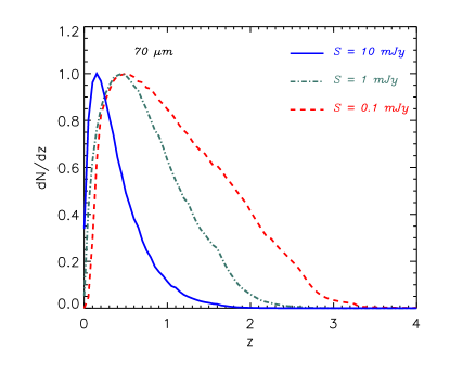
Figure 7: The modeled redshift distribution of objects which are observed with different flux thresholds at $70\,\mu$m (in the left panel) and $850\,\mu$m (in the right panel). Three different flux thresholds which are $0.1$, $1$ and $10$mJy are shown respectively using solid(blue), dot-dashed (green) and dashed (red) lines.

Moreover, there are additional physical processes, like AGNs, which can change the energy output of galaxies at shorter wavelengths. Since we do not take into account AGNs as a separate population, our model is not expected to reproduce necessarily good results for wavelengths shorter than $60-70\,\mu$m (see also the discussion in Section 2.3). Going from longer to shorter wavelengths, the observed sources are typically at lower and lower redshifts. Consequently, the source counts at short wavelengths are only sensitive to the very low redshift properties of our model. In fact, the $70\,\mu$m source count is mainly sensitive to the growth rate of the luminosity evolution, $n$, and the evolution in LF slopes; but by going to longer wavelengths, the colour evolution and the redshift at which the luminosity evolution is peaking, $z_{a}$, become more important. In other words, if a model reproduces the observed source counts at short wavelengths, this forms a confirmation that the evolution at low redshifts is represented correctly but for a best-fit model constrained by observations at shorter wavelengths, the properties of model at intermediate and high redshifts are not strongly constrained.

$\lambda$	$n$	$w$	$a_{\alpha}$	$a_{\beta}$
$850\,\mu$m	2.0	2.0	0.6	0.4
$500\,\mu$m	2.6	3.8	0.0	0.6
$350\,\mu$m	3.0	4.4	-0.2	1.4
$250\,\mu$m	3.0	4.4	0.0	1.4
$160\,\mu$m	2.2	4.2	0.8	0.2
$70\,\mu$m	2.2	2.0	0.6	0.6

Table 2: Parameters which define different best-fit models constrained to reproduce the observed source counts at different wavelengths. The first column, $\lambda$, indicates the wavelength for which the model is constrained to produce the best fit to the observed source counts. All the models are forced to reproduce the redshift distribution of submm galaxies and therefore use $z_{a}=1.6$, $z_{b}-z_{a}=1$ and $m=-1$. The predicted source count each of those models is implying for different wavelengths is illustrated in Figure 8

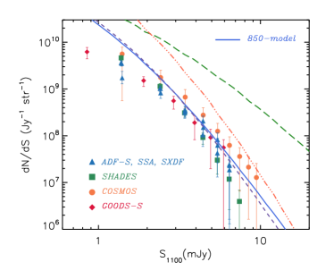
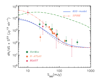
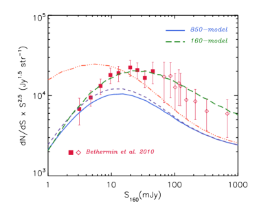
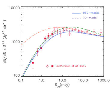
Figure 8: In different panels, the best-fit model predictions for cumulative source counts at $850\,\mu$m and differential source counts at $1100$, $500$, $250$, $160$ and $70\,\mu$m are plotted next to the observed data. The $1100\,\mu$m observational data sets are from Scott et al. (2010) (red diamonds) Austermann et al. (2009, 2010) (orange circles and green squares respecitvely) and Hatsukade et al. (2011) (blue triangles); data at $850\,\mu$m is from Coppin et al. (2006)(green triangles), Knudsen et al. (2008) (red circles) and Johansson et al. (2011) (orange squares). The data for $500$ and $250\,\mu$m source counts are from the BLAST experiment taken from Patanchon et al. (2009) (red diamonds), Herschel data taken from Oliver et al. (2010) (green squares) and Clements et al. (2010) (orange circles). We also used one data point at $350\,\mu$m from the SHARC2 survay (green triangle)(Khan et al., 2007). The data at $160$ and $70\,\mu$m are based on Spitzer observations taken from Bethermin et al. (2010) where the data points shown by filled squares represent stacking results. Different lines correspond to the source counts produced by various models which are constrained to fit the observed source counts at different wavelengths: blue solid line shows the ”850-mode”, purple dashed line shows the ”70-model” and green long-dashed and orange dot-dot-dashed lines are for ”160-model” and ”500-model” respectively (see Table 2)

To investigate the performance of different best-fit models constrained by source count observations of wavelengths other than $850\,\mu$m, we use the same procedure we incorporated in finding the “850-model” and only vary the effective parameters of the model, namely $n$, $w$, $a_{\alpha}$ and $a_{\beta}$, to fit the observed data. The parameters which define best-fit models at different wavelengths are shown in Table 2 and the source counts they produce at different wavelengths are illustrated next to the observational data points in Figure 8. Different panels are for source count at different wavelengths ranging from $1100\,\mu$m on the top left to $70\,\mu$m on the bottom right. We do not show the results for $350\,\mu$m to maintain the symmetry of figures since for this wavelength models and their comparison with observed data are in many respects identical to the case of $250\,\mu$m. In Figure 8, the source counts produced by different models are also shown using lines with different styles and colours: purple short-dashed for $70\,\mu$m, green long-dashed for $160\,\mu$m, orange dot-dot-dashed for $500\,\mu$m and finally solid blue lines for $850\,\mu$m (i.e the ”850-model”). In the following we discuss those results by categorizing them in different wavelength ranges, namely $850\,\mu$m and $1100\,\mu$m as long submm wavelengths, $500\,\mu$m, $350\,\mu$m and $250\,\mu$m as SPIRE or intermediate wavelengths and finally $70\,\mu$m and $160\,\mu$m as short wavelengths.

5.1 Long submm wavelengths: $850\,\mu$m and $1100\,\mu$m

As we mentioned earlier, the SED of star forming galaxies at long submm ranges is essentially controlled by the Rayleigh-Jeans tail of the dust emission which simply falls off smoothly (see Figure 1). This means that if a model reproduces the observed counts at $850\,\mu$m, a good fit to the observed counts at similar and longer wavelengths is guaranteed that given the distribution of sources which produce those counts have a similar redshift distributions, which in turn makes those counts equally sensitive to different parameters in our model. As illustrated in the top panels of Figure 8, both models which are constrained by observed $70\,\mu$m and $850\,\mu$m counts and produce a good fit to $850\,\mu$m data, also produce a good fit to $1100\,\mu$m source counts. Our experiments with other models also confirm that the quality of the fit they produce for observed counts at $850\,\mu$m and $1100\,\mu$m is highly correlated. Both of the models constrained by $160\,\mu$m and SPIRE (e.g. $500\,\mu$m) source counts over produce the long submm wavelength source counts: the ”160-model” over-produces submm source counts mainly at bright flux thresholds due to its extreme colour evolution (see Table 2) but fits the observations at faint fluxes, thanks to its luminosity evolution which is similar to those of ”850-model” and ”70-model”. However, SPIRE constrained models (e.g. ”500-model”) have stronger evolutions both in terms of luminosity and colour and over-produce the data in all observed fluxes.

One should note that the $1100\,\mu$m data points are highly incomplete below $3$mJy (Hatsukade et al., 2011) and are prone to large field to field variations and relatively large errors in the whole range of observed fluxes. Moreover, the observed counts are at bright flux thresholds which makes them sensitive to a narrower redshift interval in comparison to the fainter flux thresholds (see the right panel of Figure 7) and because of those reasons they cannot constrain models better than what $850\,\mu$m source counts are capable of. Therefore, we only consider the ”850-model” as a model constrained by long submm source counts.

5.2 SPIRE intermediate wavelengths: $500\,\mu$m, $350\,\mu$m and $250\,\mu$m

The three $500\,\mu$m, $350\,\mu$m and $250\,\mu$m wavelengths are close together and besides being in the middle of wavelength ranges we study, they have intermediate properties with respect to the redshift range each wavelength is mostly sensitive to: as it is shown in Figure 10, while at the bright flux thresholds the source counts mainly consist of low redshift sources, at fainter fluxes they are sensitive to the intermediate (i.e. $1<z<2$) and high redshifts (i.e. $2<z$). Naturally the general behavior of models for $500\,\mu$m is closer to $850\,\mu$m while $250\,\mu$m is close to shorter wavelengths. However, those intermediate wavelengths are closely similar to each other more than being similar to other wavelengths. Consequently, the best-fit models constrained by SPIRE wavelengths have similar parameters ( 250-model and 350-model have almost identical parameters) and any of those models agrees with the observed source counts of the other two. However, SPIRE-constrained models all require steep luminosity evolution and strong colour evolution in addition to a steepening bright end slope of the LF with redshift (i.e. positive $a_{\alpha}$ together with almost zero $a_{\beta}$, see Table 2). The first two mechanisms produce too many objects in comparison to what is needed for the source counts at other wavelengths while the steeper bright end of the LF partially compensate the over-production of bright objects: as is shown in Figure 8, SPIRE-constrained models over-produce the faint source counts both at longer and shorter wavelengths but the steep bright end of LF produces results which are close to the observed faint source counts at very long wavelengths (i.e. $850\,\mu$m and $1100\,\mu$m) which in turn is too strong to leave enough sources required for the bright $160\,\mu$m sources. As we will discuss later, it is not surprising that SPIRE-models agree with bright $70\,\mu$m counts since they are essentially $z\sim 0$ objects for which evolutionary mechanisms in the model barely have any effect.

While the SPIRE models fail to agree with observations at shorter and longer wavelengths, the two models which are successful at long submm ranges (i.e. the ”850-model” and ”70-model”) also have a reasonable agreement with the SPIRE data. However, they under-produce the counts at $S_{th}<100$mJy by a factor of $\sim 2$. As we will show later, assuming the ”850-model” to be correct, this under-production is a hint for a population of cold luminous IR galaxies residing only in low and intermediate redshifts (i.e. $z\sim 1$). This is also consistent with the steep coluor evolution which is implied by best-fit models at those wavelengths which produces enough cold galaxies at lower redshifts.

5.3 Short wavelengths: $160\,\mu$m and $70\,\mu$m

At short wavelengths like $70\,\mu$m, the K-correction is not strong enough to counteract the effect of cosmological dimming which makes the source counts at these wavelengths almost insensitive to the properties of IR galaxies at high redshift. Since the starting point of our model is the observed distribution of IRAS galaxies which are selected to be local galaxies with $S_{60\,\mu{\rm{m}}}>1{\rm{Jy}}$, and the SED templates we use are extensively tested to match these galaxies, any variation of our model by construction cannot disagree with bright $70\,\mu$m counts . However, at fainter flux thresholds (e.g. $S_{th}<100$mJy) the sensitivity of $70\,\mu$m counts to low and intermediate redshifts, $0.5<z<2$, increases (see Figure 10) which makes them more sensitive to the slope of the luminosity evolution. As a result, all the models agree with $70\,\mu$m observations at bright flux threshold while the SPIRE-model which has steeper luminosity evolution (i.e. greater $n$, see Table 2) diverges from observed counts and over-produces them. It should be noted that the ”70-model” which is tuned to agree with mainly low-z IR sources performs as good as ”850-model” in longer wavelengths.

At $160\,\mu$m, the redshift distribution of sources is almost identical to the distribution of galaxies which are responsible for $70\,\mu$m: the bright end of the counts is governed by local IR galaxies while for flux thresholds $S_{th}<100$mJy the intermediate redshifts (i.e. $0.5<z<2$) become important. However, the flux threshold at which the turn over between domination of local and farther sources happens is one order of magnitude higher for $160\,\mu$m sources (see bottom row in Figure 10). Moreover, at $160\,\mu$m the domination of intermediate redshift sources in shaping the faint source counts is slightly stronger than at $70\,\mu$m. In other words, the $160\,\mu$m source counts are slightly more sensitive to the distribution and evolution of distant IR galaxies in comparison to $70\,\mu$m counts.

The best-fit model which is constrained by $160\,\mu$m source counts has similar slope of luminosity evolution, $n$, compared with the ”850-model” and ”70-model” but requires much stronger colour evolution and larger fraction of bright objects (i.e. steeper faint end slope and flatter bright end slope of LF at higher redshifts).

The SPIRE-models on the other hand, violate the observed $160\,\mu$m counts by under-producing them at bright end and over-producing them at faint fluxes. The ”850-model” and ”70-model” on the other hand, match the faintest $160\,\mu$m count but under produce the brighter objects by a factor of $\sim 2$ which is the same factor showing up in the difference between what those two models produce and observed faint SPIRE counts. A similar discrepancy between models and $160\,\mu$m counts has been pointed out in some recent works (Le Borgne et al., 2009; Valiante et al., 2009); while the Le Borgne et al. (2009) best-fit model which produces correct source counts at $70\,\mu$m and $850\,\mu$m deviates from observations between $10{\rm{mJy}}<S_{160}<100$mJy by a factor of $\sim 2$, the Valiante et al. (2009) model underestimates number counts at $160\,\mu$m by a factor of $\sim 5$. We discuss this issue further in 5.4.

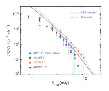
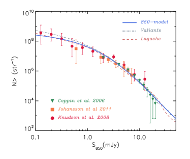
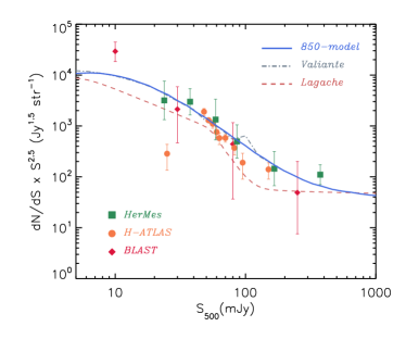
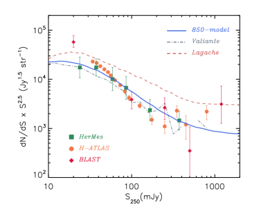
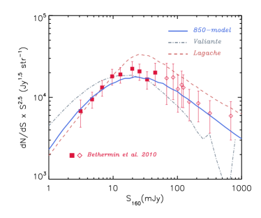
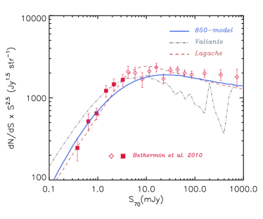
Figure 9: The same set of observed source counts which is shown in Figure 8 is also illustrated here. The blue solid line shows the result of ”850-model” using a modified set of SED (see Section 5.4) to correct under-production of bright $160\,\mu$m sources and faint SPIRE source. Source count produced by two different models, Lagache et al. (2004) and Valiante et al. (2009), are also respectively shown by orange dashed line and gray dot-dashed lines. While Valiante et al. (2009) and ”850-model” counts at $160\,\mu$m are almost identical, we did not find Lagache et al. (2004) model predictions at $1100\,\mu$m to include them in the top-left panel.

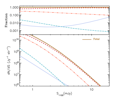
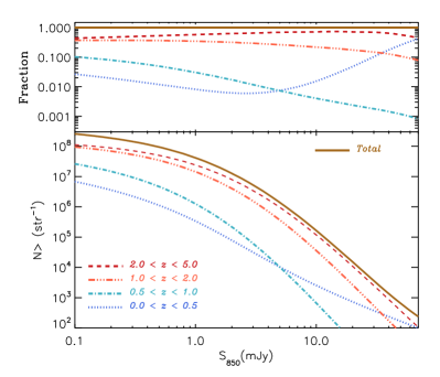
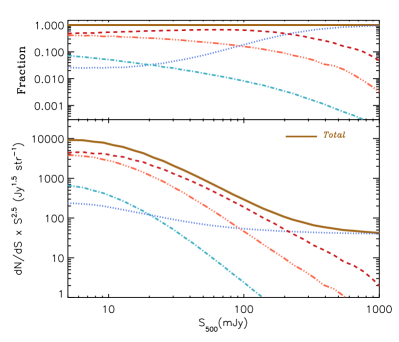
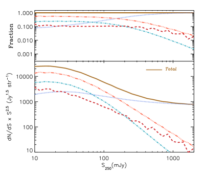
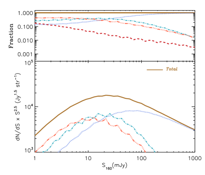
Figure 10: The fractional contribution of sources in different redshift bins in producing the observed source counts at different wavelengths are illustrated. The blue Dotted, cyan dot-dashed, orange dot-dot-dashed and red dashed lines respectively show the source count produced by objects in $0<z<0.5$, $0.5<z<1$, $1<z<2$ and $2<z<5$ redshift intervals while the total source count is shown using the brown solid line. In the top section of each panel, the fraction of sources for each redshift bin in producing source counts at different flux thresholds is plotted.

5.4 A best-fit model for all wavelengths

As we showed in previous subsections, the required evolution scenarios for different models which are constrained by various wavelengths is too diverse to be reconciled in a single model; however, the $70\,\mu$m and $850\,\mu$m source counts can be explained by the same model, either the ”850-model” or ”70-model” which are almost identical in terms of implied evolution and distribution of IR galaxies and predicted source counts at different wavelengths. While $70\,\mu$m source counts are produced mainly by local and low redshift objects, $850\,\mu$m sources are distributed in higher redshifts and in a wide redshift interval. This means the model which can explain the source count at both $70\,\mu$m and $850\,\mu$m gives a consistent distribution of IR galaxies from local Universe to very high redshifts. In other words, the same evolution scenario for star-forming galaxies which we observe locally, can also produce the observed $850\,\mu$m counts. This scenario, contrary to what is implied by the best-fit models constrained at other intermediate wavelengths, does not strongly violate observed source counts at other bands, though it under-produces them at some flux thresholds. On the other hand, models which agree with observations at intermediate wavelengths require extreme color evolutions to produce larger number of cold objects in intermediate redshift ranges which is relevant for the source count at those wavelengths (i.e. $1<z<2$, see the left panel in the middle of Figure 10). However, this steep colour evolution at higher redshifts (i.e. $z>2$) produces too many observable sources at $850\,\mu$m.

Moreover, as we mentioned earlier different authors with fundamentally different models have reported inconsistencies in their best-fit models (which fit the long and short wavelengths) and intermediate source counts (Le Borgne et al., 2009; Valiante et al., 2009) and the underestimation of $160\,\mu$m (and SPIRE wavelengths) seems to be model independent.

There are two main possibilities which can explain the origin of discrepancy between the ”850-model” and source counts at SPIRE band and $160\,\mu$m, besides doubting the validity of observed counts: (i) the IR SEDs in our model are not representative and should be modified in a certain way to produce more flux at observed wavelengths $\lambda_{obs}\sim 160$ - $500\,\mu$m or (ii) existence of a population of cold galaxies at relatively low redshifts. Indeed, there is a body of evidences supporting a population of cold galaxies which are underrepresented in IRAS galaxies and hence $70\,\mu$m source counts (Stickel et al., 1998, 2000; Chapman et al., 2002; Patris et al., 2003; Dennefeld et al., 2005; Sajina et al., 2006; Amblard et al., 2010). However, based on available data there is no possible way to disentangle between the two mentioned possibilities (Le Borgne et al., 2009). Therefore, due to its simplicity, we try to find a modification in SED amplitudes which could improve the agreement between the ”850-model” and observed source counts at SPIRE wavelengths and $160\,\mu$m, without affecting other wavelengths. In the following we first introduce the desired SED modification and then based on the redshift distribution of sources responsible for different source counts in our modified model, we try to constrain different properties a population of cold IR galaxies should possess to be equivalent to that SED modification.

Since the ”850-model” is capable of fitting the observed $70\,\mu$m source counts, any modification of SED templates should be at wavelengths longer than $70\,\mu$m to leave this agreement intact. The $850\,\mu$m source counts that model produces should also remains the same which put an upper limit for the allowed wavelength range of any modification: since a significant fraction of observed counts at $850\,\mu$m is produced by sources at high redshifts, typically $z>2$ (see Figures 7 and 9), SED templates should not change at rest-frame wavelengths longer than $\sim 200\,\mu$m. Based on this ansatz, we searched for the amplitude and the wavelength range of SED changes which can bring the ”850-model” intermediate wavelength counts close to the observed values. We found that if the SED templates we use in our model be amplified by a factor of $1.6$ in the rest-frame range of $70<\lambda<150\,\mu$m, the ”850-model” can fit the SPIRE and $160\,\mu$m source counts, without any change in already decent results at $70\,\mu$m, $850\,\mu$m and $1100\,\mu$m. Figure 9 illustrates the results produced by this modified ”850-model” at different wavelengths (blue solid line) together with the results from Lagache et al. (2004) (orange dashed line) and Valiante et al. (2009) (gray dash-doted line) models. The redshift distribution of sources responsible for those results are also shown in Figure 10.

The SED boost we implemented, recovers the observed $160\,\mu$m counts by doubling the number of observable sources with $S_{160}>10{\rm{mJy}}$; as illustrated in Figure 9, a significant fraction of those sources is distributed at redshifts $z<1$ which is also in agreement with recent observations (Jacobs et al., 2011; Berta et al., 2011). However, for the SPIRE source counts, the SED modification increases the number of observed sources with $S_{\rm{SPIRE}}<100{\rm{mJy}}$ which are mainly at redshifts $0.5<z<2$. Those redshift distributions together with the fact that the emission from cold dust with temperatures $T\lesssim 30$K peaks at $\sim 100\,\mu$m, make our SED modification equivalent to adding a population of preferentially cold dusty galaxies which do not exist at high redshifts. The width of redshift range in which those objects can exist depends on their temperature range: a warmer population can have a wider redshift distribution but should have a typically higher redshifts to be invisible at $70\,\mu$m while a colder population can only exist in low redshift ranges in order to not interfere with $850\,\mu$m counts. Interestingly, this is in agreement with the required steep colour evolution implied by models constrained by $160\,\mu$m and SPIRE band counts (see Table 2).

As one can see in Figure 9, some models like Lagache et al. (2004) and Valiante et al. (2009) not only produce enough observable sources in SPIRE and $160\,\mu$m bands, but at some flux thresholds produce too many sources. However, we notice that both of those models need an additional mechanism to compensate for under-production of visible sources at intermediate wavelengths which mimic a population of cold sources only in low redshifts. For instance, Lagache et al. (2004) use a class of ”cold galaxies” in their evolutionary model which are present only at low redshift, $z<0.5$; Lagache et al. (2003) show that this cold population is producing up to $\sim 50\%$ of the observed $170\,\mu$m flux which means without them the source count is reduced by the same factor, consistent with our finding and also other models (Le Borgne et al., 2009; Valiante et al., 2009). Similarly, Valiante et al. (2009) need to strongly modify the colour distribution of low redshift galaxies to correct for under-producing $160\,\mu$m sources by a factor of $\sim 5$; they modified the observed colour distribution of IRAS galaxies which they use as starting point (similar to our model, see Section 2.1) only for low redshift (i.e. $z<1$) objects, by assuming an asymmetric Gaussian distribution which is 7 times broader on the ”cold” side of distribution in comparison to the ”warm” side (see Section 4.4 in Valiante et al. (2009)); even with this extreme modification their model does not completely match the observed $160\,\mu$m counts in addition to under-producing luminous $70\,\mu$m sources.

Finally, it is worth mentioning that our SED modification is not expected to change the best-fit models which are based on $70\,\mu$m and $850\,\mu$m since we used those source counts as constraints for our SED change search. However we double checked this issue by using the modified SED set and repeating the search in parameter space for a best-fit model which is constrained by source counts at $70\,\mu$m, $160\,\mu$m, SPIRE bands and $850\,\mu$m and recovering the parameters which define the ”850-model”, for the best-fit model.

6 Discussion

In this section, we discuss different properties of our best-fit model. First we discuss different implications of our model for the evolving properties of the IR galaxies like their colour and luminosity distributions. Then, we compare our model with other existing models for IR and submm source counts.

6.1 The implied evolution scenario for dusty galaxies

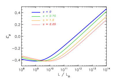
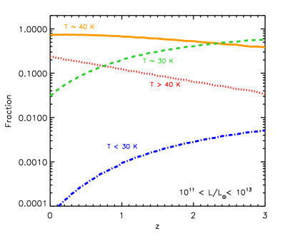
Figure 11: Top: The evolution of CF (left) and LF (right) with redshift. The lines from thick to thin are respectively for redshifts $z=$ 0 (blue), 0.75 (green), 1.5 (orange) and 2.25 (red). Bottom: The change of the relative contribution of different populations of IR galaxies to their total density with redshift, as required to reproduce the observed source counts correctly. left: The fraction of objects with luminosities $10^{11}\leq L/L_{\odot}\leq 10^{13}$ which have typical temperatures of $T<30$ K, $\sim 30$ K, $\sim 40$ K and $T>40$ K shown respectively with blue, green, orange and red lines. right: The fraction of total IR luminosity generated by objects with luminosities $10^{10}\leq L/L_{\odot}\leq 10^{13}$, which have luminosities of $10^{10}\leq L/L_{\odot}<10^{11}$, $10^{11}\leq L/L_{\odot}<10^{12}$ and $10^{12}\leq L/L_{\odot}\leq 10^{13}$ shown respectively with red, green and blue lines.

Our best-fit model mimics the number density evolution of IR galaxies by employing a luminosity evolution together with changing slopes of LF with redshift. While the former changes the amplitude of LF, the latter acts to change the shape of LF properly to reproduce a number density history which matches the observed FIR and submm source counts. Although the good agreement between source counts which our best-fit model produces at different wavelengths and the observed numbers firmly supports our model, the implied results should be treated carefully, mainly due to the simplicity of the model: for instance, in our model we adopted the local LF of IR galaxies which is a simple dual power law function, and evolved its characteristic luminosity and slopes with redshift to distribute objects with different luminosities in redshift space correctly.

Although the functional forms we chose for evolution of those parameters are rather arbitrary, the actual distribution they produce at different redshifts is necessary to explain the properties of the observed sources. To emphasize this point, in Figure 11 we illustrate how the fractions of galaxies in different luminosity bins are evolving with redshift, together with the exact shape of the LF our model requires at different redshifts. As can be seen in the bottom right panel of Figure 11, at low redshifts fainter objects dominate the population of IR galaxies but at higher redshifts (i.e., $z>2$), objects which are in brighter luminosity ranges take over and become more dominant. Specifically, this diagram shows that beyond $z\sim 1$, objects in the Luminous Infrared Galaxies (LIRGs) class (with IR luminosities between $10^{11}$ and $10^{12}\,L_{\odot}$) dominate the obscured cosmic energy production (although in terms of numbers, fainter galaxies still dominate). The diagram also shows that UltraLuminous Infrared Galaxies (ULIRGs, with IR luminosities exceeding $10^{12}\,L_{\odot}$), although increasing in importance towards high $z$, never dominate the cosmic energy production. These conclusions are in agreement with analyses of Spitzer data by Le Floc’h et al. (2005) for $z<1$ and by Magnelli et al. (2011) for $z<2.3$.

Our best-fit model implies a change in the shape of the LF with redshift and we are the first to consider this possibility in a model of this type. This slope evolution implies that the faint end slope of the LF is flattening with increasing redshift (see the top right panel of Figure 11). At first sight it may seems surprising that our results are sensitive to the faint end slope at high redshifts, but the strong luminosity evolution combined with the strong negative $K$-correction brings sub-$L_{*}$ galaxies well within the region of detectability at $850\,\mu$m. Nevertheless, this result depends strongly on the sub-mJy counts at $850\,\mu$m which currently are derived from studies of gravitationally lensing clusters, and therefore sample limited cosmic volume. As such, these counts may be affected by cosmic variance and establishing their levels more firmly (e.g., with ALMA), is necessary for confirming our conclusion. However, we note the non-parametric estimates of the IR luminosity function at high redshifts (e.g., Chapman et al., 2005; Wardlow et al., 2011) do indicate flatter faint-end slopes than the local LF. These samples were selected at $850\,\mu$m and may not be complete in IR luminosity, in particular they may be deficient in objects with high dust temperatures (e.g., Magdis et al., 2010). In order to settle this point, high-$z$ luminosity functions of IR luminosity-limited samples are required. Redshift surveys of Herschel-selected samples will be needed to construct such luminosity functions, and this will become feasible with facilities such as ALMA and CCAT. If confirmed, the flattening of the faint-end slope of the LF towards higher redshifts requires a physical explanation, which perhaps could be found using physically motivated models and simulations. One possibility is that a higher metagalactic ultraviolet flux at higher redshifts would suppress the development of a star-forming interstellar medium in low-mass galaxies. Another possibility is a stellar-mass-dependent evolution in $M_{\rm dust}/M_{\rm stars}$ towards higher redshifts. Such an evolution could result from the decreasing overall metallicity towards high $z$ combined with the net effect over time of the buildup of dust as a result of stellar evolution and its consumption by star formation. The latter model can be tested observationally using a combination of Herschel data and multi-band optical imaging (Bourne et al., in prep.).

We also showed that our model requires a colour evolution to reproduce the observed source counts. This colour evolution implies that objects with the same luminosities have lower typical dust temperatures at higher redshifts. In the bottom left panel of Figure 11 we showed how the fraction of objects with different temperatures is evolving with redshift for all the objects which have intrinsic luminosities between $10^{11}<\frac{L}{L_{\odot}}<10^{13}$. While at low redshifts a population of objects which have typical temperatures of $40$K, dominates the colour distribution, at higher redshifts the cooler typical temperature of $30$K is dominating. Moreover, while at low redshifts objects with warm dust temperatures are more common than the very cold objects, the situation is the opposite at earlier times. Although it is difficult to observe the evolution of dust towards cooler temperatures because of different selection effects, there is observational evidence for the implied colour (i.e., temperature) evolution (Chapman et al., 2005; Pope et al., 2006; Chapin et al., 2009; Symeonidis et al., 2009; Seymour et al., 2010; Hwang et al., 2010; Amblard et al., 2010).

The luminosity and colour evolutions discussed above, show up in redshift distributions of source counts at different wavelengths. Figure 10 illustrates the buildup of source counts at different wavelengths by contribution from different redshift bins. It is evident that the longer wavelengths are reflecting the distribution of higher redshift dusty galaxies while shorter wavelengths depend more on IR galaxies at lower redshifts. For instance $850\,\mu$m number counts mainly consist of galaxies with redshifts higher than $z\sim 2$, especially at fluxes $\sim 10-20{\rm{mJy}}$; in addition, as shown in the bottom right panel of Figure  11, at redshifts $z\sim 2$ the luminosity distribution of IR galaxies is not evolving considerably and even at higher redshifts the fraction of fainter sources, which have lower dust temperatures, goes up again in comparison to the brightest objects. Moreover, for two objects with the same redshifts and intrinsic IR luminosities, the colder one will be brighter at observed $850\,\mu$m. This means the visible $850\,\mu$m sources at higher flux thresholds are preferentially colder than sources with fainter observed fluxes which are distributed typically at lower redshifts (see the increasing fraction of objects in $1<z<2$ redshift bin going towards lower fluxes in the top right panel of Figure 10). This is also in agreement with our experiments which show that at the bright end, $850\,\mu$m number counts are very sensitive to the slope of the colour evolution in our model, which is in fact the dominant mechanism to produce those counts. Moreover, this implied broader temperature distribution of observed sources at fainter flux thresholds and shorter wavelengths is in agreement with observations which show bright $850\,\mu$m population (i.e. $>4{\rm{mJy}}$) is highly biased towards cold dust temperatures while fainter sources (i.e. $1-4{\rm{mJy}}$) also contain an increasing fraction of more luminous objects with lower redshifts but warmer dust temperatures which makes them the main contributors to the $250\,\mu$m source counts (Chapman et al., 2004, 2010; Magnelli et al., 2010; Casey et al., 2009, 2011). Consequently, at $z\sim 2$ the density of farIR selected ULIRGs is approximately 2 times higher than that of $850\,\mu$m-selected ULIRGs. This is consistent with our model: a typical ULIRG at redshift $z\sim 2$ will be visible at $850\,\mu$m with a flux brighter than a few mJys and at $250\,\mu$m brighter than $\sim 100$mJy; on the other hand, roughly $\sim 20-30\%$ of objects with few mJy fluxes at $850\,\mu$m are within redshifts $z\sim 1-2$ while around $\sim 50\%$ of objects with $\sim 100$mJy fluxes at $250\,\mu$m are in the same redshift bin (see Figure 10).

While the luminosity and colour distribution our best-fit model requires is consistent with observed $70\,\mu$m, $850\,\mu$m and $1100\,\mu$m source counts, they are not sufficient to produce enough sources at observed wavelengths in between. The inconsistency between models which successfully produce $70\,\mu$m and $850\,\mu$m counts and their results at $160\,\mu$m, is also reported in other works and has been corrected by including a population of cold galaxies at low redshifts (Lagache et al., 2003, 2004; Le Borgne et al., 2009; Valiante et al., 2009). While it is important to note the under-production of $160\,\mu$m counts in models, can be corrected equally by a modifying SED templates instead of introducing a new population (see also Le Borgne et al. (2009)), there is some observational evidence for the existence of a cold population at low redshifts which is under-represented in IRAS sample and is often associated with bright spiral galaxies(Stickel et al., 1998, 2000; Chapman et al., 2002; Patris et al., 2003; Dennefeld et al., 2005; Sajina et al., 2006; Amblard et al., 2010).

Recently, flux density measurements at 250, 350 and $500\,\mu$m have become available for large samples of local galaxies from surveys with SPIRE on the Herschel Space Observatory (Eales et al., 2010; Oliver et al., 2010; Clements et al., 2010). In addition to problems at $160\,\mu$m, we also noticed the inconsistency between our best-fit model and the source counts provided by SPIRE observations. However, we resolved this issue by modifying our SED templates to be able to reproduce the source count simultaneously at $70\,\mu$m, $160\,\mu$m, SPIRE band, $850\,\mu$m and $1100\,\mu$m. There is also observational evidence for a population of cold galaxies residing at low redshifts (equivalent to modified SEDs) in Herschel-selected samples: using a subsample with spectroscopic or reliable photometric redshifts from Herschel ATLAS survey, Amblard et al. (2010) performed isothermal graybody fits to low-redshift galaxies detected from 70 to $500\,\mu$m, resulting in an IR luminosity-temperature relation offset to significantly lower temperatures when compared to the IRAS-based relation derived by Chapman et al. (2003). The new relation found by Amblard et al. (2010) is consistent with earlier work by Dye et al. (2009) based on BLAST data. It is also important to realize that these results do not imply that the IRAS-based dust temperature fits are incorrect (in fact, they are often supplemented with measurements at longer wavelengths) but they imply that an IRAS-based selection is biased towards warmer objects.

6.2 Our best-fit model and previous models

There are several phenomenological models in the literature which try to reproduce the properties of IR galaxies at different wavelengths, with different levels of complexity (e.g., Blain & Longair (1993); Guiderdoni et al. (1997); Blain et al. (1999); Chary & Elbaz (2001); Rowan-Robinson (2001); Dole et al. (2003); Lagache et al. (2004); Lewis et al. (2005); Le Borgne et al. (2009); Valiante et al. (2009)). In general, those models use an assumed form of luminosity evolution together with a density evolution to mimic the evolution of IR galaxy distributions. However, we have limited ourselves to a pure luminosity evolution with no density evolution, and as pointed out in Section 2.2, the amount of density evolution allowed by the integrated CIB is small but does not have to be zero. On the other hand, we use evolving faint and bright ends slopes in our luminosity function. At first sight this may looks a simple substitution of free parameters; we tried to investigate this by trying to substitute the slope evolution of our model with a density evolution. However, the resulting fit with density evolution and in absence of slope evolution is significantly inferior to the fit obtained with pure luminosity evolution.

Another usual practice in modeling the infrared and submm source counts is to use only one or a few SED templates to represent the whole galaxy population. This approach neglects the observed colour distribution of local IR galaxies and do not leave any possibility for colour evolution. However, similar to Valiante et al. (2009), in our model we use a complete set of SED templates which are shown to be representative of local IR galaxies. This choice enabled our model to explore the evolution in colours of IR galaxies in addition to their luminosities.

Our model also differs from other works in the literature in calculating the source counts for a given evolutionary scenario: we calculate the source count for a given model by computing the probability of observing different sources for different flux thresholds. The direct consequence of this new approach is a fast calculation routine which enables us to calculate the source counts at very bright observed fluxes, where Monte-Carlo based methods are very inefficient due to the rarity of such objects, and therefore sometimes end up with very noisy results (see the bright source counts produced by Valiante et al. (2009) in Figure 9). Moreover, our fast algorithm is an important advantage when it comes to searching the parameter space for the best-fit model.

A comparison between our best-fit model and Lagache et al. (2004), as a model without colour distribution and evolution and Valiante et al. (2009) as a model with colour distributions is shown in Figure 8. While at $1100\,\mu$m, Valiante et al. (2009) produces $\sim 2$ times more visible objects than what our model produces, all models do reasonably well in accounting for the comulative $850\,\mu$m number counts. The results from Valiante et al. (2009) and our model are very close at SPIRE wavelengths but the Lagache et al. (2004) model overpredicts the bright counts at $250\,\mu$m. At $160\,\mu$m, the Valiante et al. (2009) model over-produces the faint counts and under-produces the bright objects. However, Lagache et al. (2004) fit the data better, while slightly over-produces the counts for intermediate to bright flux thresholds. Finally, at $70\,\mu$m, where all the models are expected to fit the data since they use it as a starting point, the Valiante et al. (2009) source counts deviate from observations by over-producing the faint counts in expense of producing too few bright objects (probably because of a too extreme modification in colour distributions which is required in their model to compensate for a factor of $\sim 5$ under-production of $160\,\mu$m sources).

7 Conclusions

We have described a backward evolution model for the IR galaxy population, with a small number of free parameters, emphasizing which parameters are constrained by which observations. We also introduced a new algorithm for calculating source counts for a given evolutionary model by direct integration of probability distributions which is faster than using Monte-Carlo sampling. This is an important advantage for searching large volumes of parameter space for the best-fit model.

While most of the earlier works used only one or a handful of SED templates to represent the whole population of IR objects, we used a library of IR SEDs which are able to match the IR properties of the large variety of observed star-forming objects. This approach is necessary in order to model the colour evolution of IR galaxies in addition to produce simultaneously the counts and the redshift distributions at wavelengths shorter than $850\,\mu$m.

Contrary to some other models, we assumed a negligible contribution from AGN in our SED templates, noting the inclusion of AGN is only necessary for reproducing the properties of IR galaxies at very short IR wavelengths which could also be sensitive to other modeling difficulties such as the PAH contribution to the SEDs.

We used available $850\,\mu$m source counts together with the redshift distribution of submm galaxies to constrain our best-fit model. At $850\,\mu$m, due to the K-correction, the source count is sensitive to the evolution of IR galaxies in a wide redshift range and out to very high redshifts. We showed that there is a degeneracy between the rate by which the characteristic luminosity of IR galaxies should increase to reproduce the source count and the maximum redshift out to which this increase should be continued; we resolve this degeneracy by requiring the model to reproduce the observed redshift distribution of submm galaxies. Moreover, we showed that our model requires a colour evolution towards cooler typical dust temperatures at higher redshifts. The employed colour evolution is similar to that used by Valiante et al. (2009) however, our best-fit model predicts a somewhat stronger colour evolution than that proposed by these authors.

Another important feature of our model is that the best-fit is obtained using pure luminosity evolution but mildly evolving high-luminosity and low-luminosity slopes in the LF. Since high-luminosity sources are rare, the evolution in the high-luminosity slope is of little consequence. However, the evolution of the low-lumuninosity slope affects large numbers of galaxies and if confirmed, this effect must have a physical origin, which can be addressed using numerical simulations of the evolution of the galaxy population, as well as with a combination of deep Herschel and optical imaging.

The $850\,\mu$m-constrained best-fit model is consistent with observed $1100\,\mu$m and $70\,\mu$m source counts, which confirm the consistency of the implied colour-lumionosity-redshift distribution at both low and high redshifts. However, this model under-produces the observed source counts at intermediate wavelengths, namely at $160\,\mu$m and SPIRE bands. To resolve this issue, we used the observed data at different wavelengths to find best-fit models which can reproduce their observed source counts. While the best-fit models constrained at $70\,\mu$m and $850\,\mu$m are consistent with each other and also $1100\,\mu$m, the implied evolutions for models capable of reproducing observed counts at other wavelengths are too diverse to be reconciled in a single model; specifically they need too strong colour evolutions which contradicts $850\,\mu$m observations. While the inconsistency at $160\,\mu$m has been reported in earlier works (Le Borgne et al., 2009; Valiante et al., 2009), we are the first to report it for $250\,\mu$m, $350\,\mu$m and $500\,\mu$m. We showed that the source counts at these wavelengths can be reproduced consistently, by adopting the best-fit model which produces correct $70\,\mu$m, $850\,\mu$m and $1100\,\mu$m source counts, together with a modification in SED templates which is equivalent to the existence of a cold population of dusty galaxies at low to intermediate redshifts which are under-represented in IRAS data. Besides the fact that there is some observational evidence for the existence of such galaxies (Stickel et al., 1998, 2000; Chapman et al., 2002; Patris et al., 2003; Dennefeld et al., 2005; Sajina et al., 2006; Amblard et al., 2010), this assumption is similar to what other models had to assume in order to reproduce adequate $160\,\mu$m sources (Lagache et al., 2003, 2004; Valiante et al., 2009).

It is important to keep in mind that phenomenological models like what we described in this paper, are mainly simple mathematical forms which relate different observations consistently rather than being physical models with explanatory power. However, their performance at different wavelengths and the distribution of sources they require for different redshifts can be used as their main predictions which also could be used to test their validity. While we used the redshift distribution of submm galaxies to constrain our model, we note that the observed redshift distribution of other wavelengths, if available, are in agreement with our best-fit model predictions (Jacobs et al., 2011; Berta et al., 2011).

Additional information including tabulated data for differential and cumulative source counts at different wavelengths and their redshift distributions is available at $\mathtt{http://www.strw.leidenuniv.nl/genesis/}$

Appendix A: Some numerical details

For each specific evolution model, the source count at a given flux threshold and wavelength can be calculated based on equation (13), where the integration should be performed over all possible luminosities, colours and redshifts. As mentioned in Section 2.4, we do this by splitting possible colour, luminosity and redshift ranges into very small bins, assuming that in each bin the related variable is not changing significantly.

The finite number of SED models we are using automatically splits the colour range into 64 bins between $0.29\leq R(60,100)\leq 1.64$ (see Section 2.3). We also use logarithmically spaced bins to split the possible luminosity range of $10^{9}L_{\odot}\leq L\leq 10^{14}L_{\odot}$ into 100 bins in our calculation. This logarithmic scale which makes the integration roughly insensitive to the number of luminosity bins, is chosen to cope with the exponential nature of luminosity function where faint objects are much more numerous than luminous ones. It is also worth mentioning that the source count calculation is not sensitive to the minimum or maximum luminosity which is used in integration, if the used luminosity range covers the important $10^{10}-10^{13}L_{\odot}$ luminosity range; for instance, using $L_{\rm{min}}=10^{7}L_{\odot}$ instead of $L_{\rm{min}}=10^{9}L_{\odot}$ as the minimum possible luminosity, does not change any of the source count calculations we are presenting in this paper.

As discussed in Section 2.4, the uniform distribution of galaxies in redshift space is assured by the algorithm we are using, independent of the size of redshift bins. But, for the precise calculation of the K-correction and evolution functions, we split the redshift range of $0\leq z\leq 8$ using bin sizes equal to $\Delta z=0.01$. However we noted it is possible to use even bigger redshift bins (e.g. $\Delta z=0.1$) without any significant change in the results.

References

- Alexander et al. (2005) Alexander D.M., et al., 2005, ApJ, 632, 736
- Amblard et al. (2010) Amblard A., et al., 2010, A&A, 518, L9
- Austermann et al. (2009) Austermann J.E., et al., 2009, MNRAS, 393, 1573
- Austermann et al. (2010) Austermann J.E., et al., 2010, MNRAS, 401, 160
- Barger et al. (1999) Barger A.J., et al., 1999, ApJ, 518, L5
- Berta et al. (2011) Berta B., et al., 2011, A&A, arXive:1106.3070
- Bertoldi et al. (2007) Bertoldi F., et al., 2007, ApJS, 172, 132
- Bethermin et al. (2010) Bethermin M., et al., 2010, A&A, 512, 78
- Bethermin et al. (2011) Bethermin M., et al., 2011, A&A, 529, 4
- Blain & Longair (1993) Blain A.W., Longair M.S., 1993, MNRAS, 264, 509
- Blain et al. (1999) Blain A.W., et al., 1999, MNRAS, 302, 632
- Borys et al. (2003) Borys, C., et al., 2003, MNRAS, 344, 385
- Casey et al. (2009) Casey C.M., et al., 2009, MNRAS, 399, 121
- Chapin et al. (2009) Chapin E.L., et al., 2009, MNRAS, 393, 653
- Chapman et al. (2002) Chapman S.C., et al., 2002, MNRAS, 335,17
- Chapman et al. (2003) Chapman S.C., et al., 2003, ApJ, 588, 186
- Chapman et al. (2004) Chapman S.C., et al., 2004, ApJ, 614, 671
- Chapman et al. (2005) Chapman S.C., et al., 2005, ApJ, 622, 772
- Chapman et al. (2010) Chapman S.C., et al., 2010, MNRAS, 409,13
- Casey et al. (2009) Casey C.M., et al., 2009, MNRAS, 399,121
- Casey et al. (2011) Casey C.M., et al., 2011, MNRAS.tmp.884C
- Chary & Elbaz (2001) Chary R., Elbaz D., 2001, ApJ, 556, 562
- Clements et al. (2010) Clements D.L., et al., 2010, A&A, 518, 8
- Coppin et al. (2006) Coppin K., et al., 2006, MNRAS, 372, 1621
- Cowie et al. (2003) Cowie K., et al., 2006, MNRAS, 372, 1621
- Dale et al. (2001) Dale D., et al., 2001, ApJ, 549, 215
- Dale & Helou (2002) Dale D., Helou G., 2002, ApJ, 576, 159
- Dennefeld et al. (2005) Dennefeld M., et al., 2005, A&A, 440, 5
- Dole et al. (2003) Dole H., et al., 2003, ApJ, 585, 617
- Dye et al. (2009) Dye S., et al., 2009, ApJ, 703, 285
- Eales et al. (2010) Eales S., et al., 2010, PASP, 122, 499
- Efstathiou et al. (1995) Efstathiou A., et al., 1995, MNRAS, 277, 1134
- Fadda et al. (2010) Fadda D., et al., 2010, ApJ, 719, 425
- Fixsen et al. (1998) Fixsen D. J., et al., 1998, ApJ, 508, 123
- Gispert et al. (2000) Gispert R., et al., 2000, A&A, 360, 1
- Greve et al. (2004) Greve, T. R., et al., 2004, MNRAS, 354, 779
- Guiderdoni et al. (1997) Guiderdoni B., et al., 1997, Nature, 390, 257
- Hatsukade et al. (2011) Hatsukade B., et al., 2011, MNRAS, 411, 102
- Hopkins & Beacon (2006) Hopkins A.M., Beacon J.F., 2006, ApJ, 651, 142
- Hwang et al. (2010) Hwang H.S., et al., 2010, MNRAS, 409, 75
- Jacobs et al. (2011) Jacobs B.A., et al., 2011, AJ, 141, 110
- Jauzac et al. (2010) Jauzac J.M., et al., 2010, A&A, sub.
- Johansson et al. (2011) Johansson D., et al., 2011, A&A, 527, A117
- Khan et al. (2007) Khan S.A., et al., 2007, ApJ, 665, 973
- Knudsen et al. (2008) Knudsen K.K., et al., 2008, MNRAS, 384, 1611
- Lagache et al. (2003) Lagache G., et al., 2003, MNRAS, 338, 555
- Lagache et al. (2004) Lagache G., et al., 2004, ApJS, 154, 112
- Lagache et al. (2005) Lagache G., et al., 2005, ARA&A, 43, 727
- Le Borgne et al. (2009) Le Borgne D., et al., 2009, A&A, 504, 727
- Le Floc’h et al. (2005) Le Floc’h E., et al., 2005, ApJ, 632, 169
- Lewis et al. (2005) Lewis G.F., et al., 2005, ApJ, 621, 32
- Lutz et al. (2005) Lutz D., et al., 2005, ApJ, 632, 13
- Magdis et al. (2010) Magdis, G.E., et al., 2010, MNRAS, 409, 22
- Magnelli et al. (2010) Magnelli, B., et al., 2010, A&A, 518, 28
- Magnelli et al. (2011) Magnelli, B., et al., 2011, A&A, 528, 35
- Menendez-Delmestre et al. (2009) Menendez-Delmestre K., et al., 2009, ApJ, 699, 667
- Mullaney et al. (2011) Mullaney J.R., et al., 2011, MNRAS, arXive:1106.4284
- Oliver et al. (2010) Oliver S.J., et al., 2010, A&A, 518, 21
- Patanchon et al. (2009) Patanchon G., et al., 2009, ApJ, 707, 1750
- Patris et al. (2003) Patris J., et al., 2003, A&A, 412, 349
- Pope et al. (2006) Pope A., et al., 2006, MNRAS, 370, 1185
- Pope et al. (2008) Pope A., et al., 2008, ApJ, 675, 1171
- Puget et al. (1996) Puget J.L., et al., 1996, A&A, 308,L5
- Rowan-Robinson (2001) Rowan-Robinson M. 2001, ApJ, 549, 745
- Saunders et al. (1990) Saunders W., et al., 1990, MNRAS, 242, 318
- Sajina et al. (2006) Sajina A., et al., 2006, MNRAS, 369, 939
- Schaye et al. (2010) Schaye J., et al., 2010, MNRAS, 402, 1536
- Scott et al. (2010) Scott K.S., et al., 2010, MNRAS, 405, 2260
- Seymour et al. (2010) Seymour N., et al., 2010, MNRAS, 402, 2666
- Smail et al. (1997) Smail I., et al., 1997, ApJ, 490, L5
- Smail et al. (2002) Smail I., et al., 2002, MNRAS, 331, 495
- Stickel et al. (1998) Stickel M., et al., 1998, A&A, 336, 116
- Stickel et al. (2000) Stickel M., et al., 2000, A&A, 359, 865
- Swinbank et al. (2004) Swinbank A.M., et al., 2004, ApJ, 617, 64
- Symeonidis et al. (2009) Symeonidis M., et al., 2009, MNRAS, 397, 1728
- Valiante et al. (2007) Valiante E., et al., 2007, ApJ, 660, 1060
- Valiante et al. (2009) Valiante E., et al., 2009, ApJ, 701, 1814
- Vieira et al. (2010) Vieira, J. D., et al., 2010, ApJ, 719, 763
- Wardlow et al. (2011) Wardlow, J. L., et al., 2011, MNRAS, tmp.917w
- Webb et al. (2003) Webb T.M., et al., 2003, ApJ, 587, 41
- Weiss et al. (2009) Weiss A., et al., 2009, ApJ, 707, 1201